download pdf version of PhD book - Universiteit Utrecht

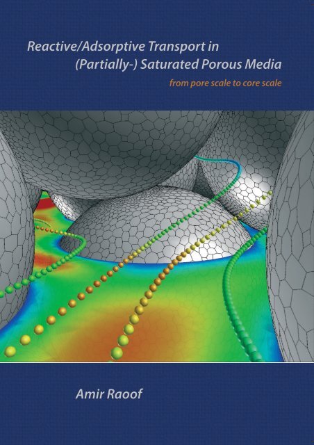
Reactive/Adsorptive Transport in 

(Partially-) Saturated Porous Media 

from pore scale to core scale 

Amir Raoof

Pore-scale modeling provides opportunities to study transport phenomena 

in fundamental ways because detailed information is available at the pore 

scale. This offers the best hope for bridging the traditional gap that exists between 

pore scale and macro (core) scale description of the process. As a result, 

consistent upscaling relations can be performed, based on physical processes 

defined at the appropriate scale. 

In the present study, we have developed a Multi-Directional Pore Net-work 

(MDPN) for representing a porous medium. Using MDPN, (partially-) saturated 

flow and reactive transport processes were simulated in detail by explicitly 

modeling the interfaces and mass exchange at surfaces. In this way, we could 

determine the upscaled parameters, and evaluate the limitations and sufficiency 

of the available analytical equations and macro scale models for prediction of 

transport behavior of (reactive) solutes. In addition, new approaches and numerical 

algorithms to accurately simulate flow and transport, under (partially-) saturated 

conditions, are developed as a FORTRAN 90 modular package. The governing 

equations are solved applying a fully implicit numerical scheme; however, 

efficient substitution methods have been applied which made the algorithm 

computationally effective and appropriate for parallel computations. 

ISBN: 978-90-3935-627

text 




Amir Raoof 

Environmental Hydrogeology Group 

Utrecht University




text 

Reactief/Adsorbtie Transport in 

te (on)verzadigde poreuze Media 

texts van Porieschaal tot Macroschaal 

(met een samenvatting in het Nederlands) 

PROEFSCHRIFT 

ter verkrijging van de graad van doctor aan de Universiteit 

Utrecht op gezag van de rector magnificus, prof.dr. G.J. van der 

Zwaan, ingevolge het besluit van het college voor promoties in het 

openbaar te verdedigen op woensdag 7 september 2011 des 

middags te 2.30 uur 

door 


geboren op 11 September 1979, te Tehran

Promoter: Prof.dr.ir. S.M. Hassanizadeh 

The Reading Committee 

Dr. Bradford, S. A., US Salinity Laboratory, USDA 

Prof. Celia, M. A., Princeton University 

Prof. Lindquist, B. W., Stony Brook University 

Prof. Rossen, W. R., TU Delft 

Prof. van der Zee, S. E. A. T. M., Wageningen University 

Copyright c○ 2011 by A. Raoof 

All rights reserved. No part of this material may be copied or reproduced in any way 

without the prior permission of the author. 

ISBN/EAN: 978-90-393-56272 

Title: 

Reactive/Adsorptive Transport in (Partially-) Saturated 

Porous Media; from pore scale to core scale 

Keywords: pore scale; reactive/adsorptive transport; Partially Saturated; 

dispersion; relative permeability, fully implicit 

numerical scheme 

Author: Raoof, A. 

Publisher: Utrecht University, Geosciences Faculty, Earth sciences 

department 

Printing: Proefschriftmaken.nl Printyourthesis.com 

NUR-code: 934 

NUR-description: Hydrologie 

Series: 

Geologica Ultraiectina 

Series Number: 300 

Number of pages: 256 

• Cover photo: Pore-scale flow simulation using CFD methods; visualization by 

John Serkowski (PNNL). 

• Cover design: Amir Raoof 

• This research was supported financially by the Utrecht Center of Geosciences 

and NUBUS international research training group.

Acknowledgements 

The acknowledgement is definitely an important part 

of the case. The case was never about moneytextttttt 

primarily. The case is about accountability.textttttttt 

Sam Dubbin 

It is a pleasure to thank several individuals who contributed to the completion 

of this study, and assisted me during its preparation. 

First and foremost, my utmost gratitude to my supervisor Majid 

Hassanizadeh. It has been an honor to be his Ph.D. student. Majid, you have 

always supported me throughout my research with your insightful knowledge 

while at the same time allowing me to work independently. I always enjoyed 

our discussions and learned so much from it. 

Furthermore, I would like to thank Ruud Schotting for all his support. I am 

grateful to Toon Leijnse and Sjoerd van der Zee from Wageningen University 

for their valuable advice on numerical simulations and pore scale modeling. A 

sincere gratitude to Scott Bradford from USDA, for reading this dissertation. 

Scott, you invited me to UC Riverside, where we had extensive discussions 

about pore scale modeling of adsorption. Your wonderful hospitality made my 

visit from Riverside unforgettable. I would also like to thank Brent Lindquist 

from Stony Brook University for his careful review and constructive comments 

on this thesis. His input greatly improved production of this book. I would like 

to show gratitude towards Mike Celia from Princeton University for very fruitful 

discussions we had during meetings and conferences. I would like to thank 

Helge Dahle, who invited me to visit University of Bergen. We had constructive 

discussions on pore scale modeling. I enjoyed being involved in NUPUS 

international research training group. I had very useful discussions with Rainer 

Helmig, and other colleagues from University of Stuttgart, during several meetings 

and throughout my visit to Stuttgart. I would like to acknowledge Hamid 

M. Nick for having useful discussions on numerical programming. 

i

My colleagues and other staff in the Hydrogeology group at UU have contributed 

immensely to my personal and professional development. The group 

has been a source of friendships, as well as good advice and collaboration. I 

would like to thank my friends: Saskia, Vahid, Nikos, Niels, Jack, Reza, Marian, 

Simona, Mariene, Brijesh, Imran, Qiu, Mojtaba, Wouter, and Shuai, as 

well as Leonid who visited our group from University of Bergen. Special thank 

to Margreet, who was of great help whenever trying to figure out all those 

administrative issues. Margreet, I always enjoyed our short talks during the 

“koffiepauze”! 

From November 2010 I have started my postdoc research, on pore scale 

modeling of reactive solutes, at the experimental rock deformation group / 

HPT-lab, Utrecht University. I would like to thank Chris Spiers for his support. 

I am enjoying my postdoc research a lot. A big thank goes to my other 

friends and colleagues in HPT-lab: Colin, Hans, Magda, André, Jon, Eimert, 

Gert, Peter, Anne, Tim, Nawaz, Elisenda, Sabine, Sander, Bart, Reinier, Loes, 

Sabrina, and Ken. 

From the time I came to Holland I was so lucky to meet many great people, 

that later became my friends. They have contributed indirectly to this study. I 

would like to mention a few in particular: Babak, Pasha, Marzieh, Vyron, Angelique, 

David, Bamshad, Baukje, Eefje, Eric, Farnoush, Rory, Lotte, Sander, 

Guillaume, Maartje, Mohammad, Moniek, Renée, Rick, Roeland, Veerle, Hajar, 

Roza, Sanaz, and Sourish. 

Lastly, and most importantly, I wish to thank my family; in particular my 

parents, Parvin and Abbass, who raised me, supported me, taught me, and 

loved me. To them I dedicate this thesis. 


Utrecht 

August 2011 

ii

CONTENTS 

List of Figures 

List of Tables 

ix 

xiv 

1 Introduction 1 

1.1 Issues of scale . . . . . . . . . . . . . . . . . . . . . . . . . . . . 2 

1.2 Continuum modeling approach . . . . . . . . . . . . . . . . . . 3 

1.3 Pore-scale modeling approach . . . . . . . . . . . . . . . . . . . 4 

1.4 Research objectives . . . . . . . . . . . . . . . . . . . . . . . . . 8 

1.5 Outline of the thesis . . . . . . . . . . . . . . . . . . . . . . . . 9 

1.6 Programming issue . . . . . . . . . . . . . . . . . . . . . . . . . 13 

I Generation of Multi-Directional Pore Network 17 

2 A New Method for Generating Multi-Directional Pore-Network 

Model 19 

2.1 Introduction . . . . . . . . . . . . . . . . . . . . . . . . . . . . . 20 

2.2 Methodology and Formulation . . . . . . . . . . . . . . . . . . . 23 

2.2.1 General Network Elements in MDPN . . . . . . . . . . 23 

2.2.2 Network Connections . . . . . . . . . . . . . . . . . . . 25 

iii

CONTENTS 

2.2.3 Connection Matrix . . . . . . . . . . . . . . . . . . . . . 26 

2.2.4 Elimination Process . . . . . . . . . . . . . . . . . . . . 26 

2.2.5 Isolated Clusters and Dead-End Bonds . . . . . . . . . . 31 

2.3 Test Cases (Optimization Using Genetic Algorithm) . . . . . . 33 

2.3.1 Generating a Consolidated Porous Medium (Sandstone 

Sample) . . . . . . . . . . . . . . . . . . . . . . . . . . . 34 

2.3.2 Generating a Granular Porous Medium . . . . . . . . . 36 

2.4 Conclusions . . . . . . . . . . . . . . . . . . . . . . . . . . . . . 37 

II 

Upscaling and Pore Scale Modeling; 

Saturated Conditions 39 

3 Upscaling Transport of Adsorbing Solutes in Porous Media 41 

3.1 Introduction . . . . . . . . . . . . . . . . . . . . . . . . . . . . . 42 

3.2 Theoretical upscaling of adsorption in porous media . . . . . . 46 

3.2.1 Formulation of the pore-scale transport problem . . . . 46 

3.2.2 Averaging of pore-scale equations . . . . . . . . . . . . . 47 

3.2.3 Kinetic versus Equilibrium Effects . . . . . . . . . . . . 51 

3.3 Numerical upscaling of adsorbing solute transport . . . . . . . 52 

3.3.1 Flow and transport at pore scale (Single-Tube Model) . 52 

3.3.2 Flow and Transport at 1-D Tube Scale . . . . . . . . . . 55 

3.3.3 Upscaled Peclet number (Pe) . . . . . . . . . . . . . . . 56 

3.3.4 Upscaled adsorption parameters (k ∗ att and k ∗ det ) . . . . . 57 

3.4 Discussion of results . . . . . . . . . . . . . . . . . . . . . . . . 61 

3.5 Conclusion . . . . . . . . . . . . . . . . . . . . . . . . . . . . . 63 

4 Upscaling Transport of Adsorbing Solutes in Porous Media: 

Pore-Network Modeling 65 

4.1 Introduction . . . . . . . . . . . . . . . . . . . . . . . . . . . . . 66 

4.1.1 Discrepancy between observations . . . . . . . . . . . . 66 

4.1.2 Pore scale modeling . . . . . . . . . . . . . . . . . . . . 67 

iv

CONTENTS 

4.1.3 Applications of pore-scale modeling to solute transport 69 

4.2 Description of the Pore-Network Model . . . . . . . . . . . . . 71 

4.2.1 Pore size distributions . . . . . . . . . . . . . . . . . . . 72 

4.3 Simulating flow and transport within the network . . . . . . . . 73 

4.3.1 Flow simulation . . . . . . . . . . . . . . . . . . . . . . . 73 

4.3.2 Simulating adsorbing solute transport through the network 74 

4.4 Macro-scale adsorption coefficients . . . . . . . . . . . . . . . . 77 

4.4.1 Dispersion coefficient . . . . . . . . . . . . . . . . . . . . 78 

4.4.2 Core-scale kinetic rate coefficients (katt c and k c det ) . . . . 79 

4.4.3 Core-scale distribution coefficient (K c ) D . . . . . . . . . 81 

4.5 Discussion . . . . . . . . . . . . . . . . . . . . . . . . . . . . . . 82 

4.6 Conclusions . . . . . . . . . . . . . . . . . . . . . . . . . . . . . 87 

III 

Upscaling and Pore Scale Modeling; 

Partially-Saturated Conditions 89 

5 A New Formulation for Pore-Network Modeling of Two-Phase 

Flow 91 

5.1 Introduction . . . . . . . . . . . . . . . . . . . . . . . . . . . . . 92 

5.1.1 Pore-network modeling . . . . . . . . . . . . . . . . . . . 92 

5.1.2 Pore-network construction . . . . . . . . . . . . . . . . . 93 

5.1.3 Objectives and approach . . . . . . . . . . . . . . . . . . 95 

5.2 Network Generation . . . . . . . . . . . . . . . . . . . . . . . . 96 


5.2.2 Determination of the pore cross section and corner half 

angles . . . . . . . . . . . . . . . . . . . . . . . . . . . . 97 

5.2.3 Coordination number distribution in MDPN . . . . . . 99 

5.2.4 Pore space discretization . . . . . . . . . . . . . . . . . . 99 

5.3 Modeling flow in the network . . . . . . . . . . . . . . . . . . . 101 

5.3.1 Primary drainage simulations . . . . . . . . . . . . . . . 101 

5.3.2 Fluid flow within drained pores . . . . . . . . . . . . . . 103 

v

CONTENTS 

5.3.3 Regular hyperbolic polygons . . . . . . . . . . . . . . . 106 

5.3.4 Calculation of relative permeability curves . . . . . . . . 108 

5.4 Results . . . . . . . . . . . . . . . . . . . . . . . . . . . . . . . . 110 

5.4.1 Flow field in the MDPN model . . . . . . . . . . . . . . 110 

5.4.2 Calculation of relative permeabilities using MDPN model 111 

5.4.2.1 Generic pore networks . . . . . . . . . . . . . . 112 

5.4.2.2 Relative permeability for a carbonate rock . . 116 

5.4.2.3 Pore Network model of Fontainebleau sandstone 118 

5.4.3 The concept of equivalent pore conductance . . . . . . . 120 

5.5 Conclusion . . . . . . . . . . . . . . . . . . . . . . . . . . . . . 122 

6 Dispersivity under Partially-Saturated Conditions; Pore-Scale 

Processes 125 

6.1 Introduction . . . . . . . . . . . . . . . . . . . . . . . . . . . . . 126 

6.1.1 Dispersion under unsaturated conditions . . . . . . . . . 126 

6.1.2 Experimental works and modeling studies . . . . . . . . 128 

6.1.3 Objectives and computational features . . . . . . . . . . 131 




angles . . . . . . . . . . . . . . . . . . . . . . . . . . . . 134 



6.3 Unsaturated flow modeling . . . . . . . . . . . . . . . . . . . . 138 

6.3.1 Drainage simulation . . . . . . . . . . . . . . . . . . . . 138 

6.3.2 Fluid flow within drained pores . . . . . . . . . . . . . . 139 

6.4 Simulating flow and transport within the network . . . . . . . . 140 

6.4.1 Flow simulation . . . . . . . . . . . . . . . . . . . . . . . 140 

6.4.2 Simulating solute transport through the network . . . . 142 

6.5 Results . . . . . . . . . . . . . . . . . . . . . . . . . . . . . . . . 145 

6.5.1 Advection-Dispersion Equation (ADE) . . . . . . . . . . 145 

vi

CONTENTS 

6.5.2 Mobile-Immobile Model (MIM) . . . . . . . . . . . . . . 148 

6.5.3 Case study . . . . . . . . . . . . . . . . . . . . . . . . . 150 

6.5.4 Relative permeability . . . . . . . . . . . . . . . . . . . 153 

6.6 Conclusion . . . . . . . . . . . . . . . . . . . . . . . . . . . . . 154 

7 Adsorption under Partially-Saturated Conditions; Pore-Scale 

Modeling and Processes 157 

7.1 Introduction . . . . . . . . . . . . . . . . . . . . . . . . . . . . . 158 

7.1.1 Major colloid transport processes . . . . . . . . . . . . . 158 

7.1.2 Experimental studies . . . . . . . . . . . . . . . . . . . . 159 

7.1.3 Mathematical models . . . . . . . . . . . . . . . . . . . 161 

7.1.4 Objectives . . . . . . . . . . . . . . . . . . . . . . . . . . 162 




angles . . . . . . . . . . . . . . . . . . . . . . . . . . . . 164 



7.3 Unsaturated flow modeling . . . . . . . . . . . . . . . . . . . . 165 

7.4 Simulating adsorptive transport within the network . . . . . . . 166 

7.5 Macro-scale formulations of solute transport . . . . . . . . . . . 169 

7.5.1 Advection-Dispersion Equation (ADE) . . . . . . . . . . 169 

7.5.2 Nonequilibrium model . . . . . . . . . . . . . . . . . . . 170 

7.6 Results . . . . . . . . . . . . . . . . . . . . . . . . . . . . . . . . 170 

7.7 Conclusion . . . . . . . . . . . . . . . . . . . . . . . . . . . . . 175 

8 Efficient fully implicit scheme for modeling of adsorptive transport; 

(partially-) saturated conditions 177 

8.1 Introduction . . . . . . . . . . . . . . . . . . . . . . . . . . . . . 178 

8.2 Numerical scheme; saturated conditions . . . . . . . . . . . . . 182 

8.2.1 Adsorption; saturated conditions . . . . . . . . . . . . . 182 

8.3 Numerical scheme; partially saturated conditions . . . . . . . . 184 

vii

CONTENTS 

8.3.1 Non-adsorptive solute . . . . . . . . . . . . . . . . . . . 185 

8.3.2 Two sites equilibrium adsorption . . . . . . . . . . . . . 187 

8.3.3 Two sites kinetic adsorption . . . . . . . . . . . . . . . . 190 

8.3.4 One site equilibrium and one site kinetic adsorption . . 192 

9 Summary and Conclusions 195 

Appendices 202 

A. Search algorithm in MDPN model . . . . . . . . . . . . . . . . 202 

B. Pore connections in MDPN model . . . . . . . . . . . . . . . . 205 

C. Averaging of pore-scale transport equation . . . . . . . . . . . . 207 

References 209 

Samenvatting 237 

viii

LIST OF FIGURES 

1.1 A network element in a Multi-Directional Pore Network. . . . . 7 

1.2 Flowchart of computational features in CPNS. . . . . . . . . . 15 

2.1 Network consisting of 8 cubes, size: N i = 3, N j = 3, N k = 3 . . 24 

2.2 Connection matrix for a network with full connections . . . . . 27 

2.3 Regular-pattern networks . . . . . . . . . . . . . . . . . . . . . 29 

2.4 Example of eliminated sites, isolated clusters, and dead-end bonds. 32 

2.5 Elimination of isolated clusters within an irregular lattice. . . . 33 

2.6 Coordination number distributions of real sandstone vs. generated 

network. . . . . . . . . . . . . . . . . . . . . . . . . . . . . 35 

2.7 Coordination number distributions of real granular porous media 

vs. generated network. . . . . . . . . . . . . . . . . . . . . . . . 37 

3.1 Conceptual representation of the Single-Tube Model. . . . . . . 53 

3.2 Breakthrough curve of concentration from Single-Tube Model. . 55 

3.3 P e p vs. Taylor dispersion . . . . . . . . . . . . . . . . . . . . . 57 

3.4 Resulting breakthrough curves from pore-scale and upscale models 58 

3.5 The relation between macro-scale kdet ∗ as a function of pore-scale 

P e p and κ. . . . . . . . . . . . . . . . . . . . . . . . . . . . . . 59 

ix


3.6 The relation between macro-scale katt ∗ as a function of pore-scale 

P e p and κ. . . . . . . . . . . . . . . . . . . . . . . . . . . . . . 60 

3.7 Upscaled distribution coefficient as a function of pore-scale dimensionless 

distribution coefficient . . . . . . . . . . . . . . . . 61 

3.8 Comparison between average concentration breakthrough curve 

and concentrations at different positions in a tube. . . . . . . . 63 

4.1 The coordination number distribution and representative domain 

of MDPN . . . . . . . . . . . . . . . . . . . . . . . . . . . 72 

4.2 The distribution of pore sizes. . . . . . . . . . . . . . . . . . . . 73 

4.3 An example of interconnected pore bodies and pore throats. . . 75 

4.4 Example of resulting breakthrough curve from the network . . 78 

4.5 Dispersion coefficient as a function of mean pore-water velocity. 79 

4.6 Detachment rate coefficient as a function of local-scale distribution 

coefficient. . . . . . . . . . . . . . . . . . . . . . . . . . . . 80 

4.7 Attachment rate coefficient as a function of local-scale distribution 

coefficient. . . . . . . . . . . . . . . . . . . . . . . . . . . . 80 

4.8 Detachment rate coefficient as a function of average pore water 

velocity. . . . . . . . . . . . . . . . . . . . . . . . . . . . . . . . 81 

4.9 Upscaled distribution coefficient, K c , as a function of local-scale 

D 

distribution coefficient, k d . . . . . . . . . . . . . . . . . . . . . . 82 

4.10 Core-scale detachment coefficient, kdet c , as a function of localscale 

distribution coefficient, k d , and mean pore-water velocity. 83 

4.11 Simulated k c det against local-scale k d. I . . . . . . . . . . . . . . 84 

4.12 Simulated k c det against local-scale k d. II . . . . . . . . . . . . . 84 

4.13 Distribution of local-scale distribution coefficient, k d . . . . . . . 86 

4.14 Core-scale detachment rate coefficient, kdet c , as a function of average 

velocity . . . . . . . . . . . . . . . . . . . . . . . . . . . . 86 

5.1 The distribution of pore-body and pore-throat sizes sizes . . . . 97 

x


5.2 The coordination number distribution and a representative subdomain 

of the MDPN . . . . . . . . . . . . . . . . . . . . . . . 100 

5.3 Connection of angular pore bodies though a pore throat . . . . 100 

5.4 Corner flow in a triangular pore throat . . . . . . . . . . . . . . 104 

5.5 The dimensionless hydraulic conductance versus corner half-angle105 

5.6 Different kinds of regular polygons with n=3,4, and 5. . . . . . 107 

5.7 relation between conductance and shape factor and number of 

vertices . . . . . . . . . . . . . . . . . . . . . . . . . . . . . . . 108 

5.8 Relation between dimensionless conductance g ∗ and ϕ for different 

number of vertices,n. . . . . . . . . . . . . . . . . . . . . . . 109 

5.9 Average velocities in different directions of MDPN . . . . . . . 111 

5.10 Scatter diagram of velocities vs. pore throat radius . . . . . . . 112 

5.11 Capillary pressure-saturation curves for three generic pore networks 

. . . . . . . . . . . . . . . . . . . . . . . . . . . . . . . . 113 

5.12 Relative permeability curves for generic pore networks . . . . . 115 

5.13 Comparison between P c − S w curves obtained from two network 

models together with the measured values . . . . . . . . . . . . 117 

5.14 Comparison between relative permeability curves obtained from 

two networks together with the measured values . . . . . . . . 118 

5.15 Coordination number distribution in MDPN and the measured 

Fontainebleau sample . . . . . . . . . . . . . . . . . . . . . . . 119 

5.16 Comparison of relative permeability computed with and without 

consideration of pore body resistance to the wetting flow. . . . 120 

5.17 Exact and approximate relative permeability curves . . . . . . 122 

6.1 Distributions of pore body and pore throat sizes . . . . . . . . 134 

6.2 The coordination number distribution and a representative domain 

of MDPN . . . . . . . . . . . . . . . . . . . . . . . . . . . 136 

6.3 Connection of angular pore bodies though a pore throat . . . . 137 

6.4 The dimensionless hydraulic conductance versus corner half-angle140 

xi


6.5 Breakthrough curve of average concentration . . . . . . . . . . 144 

6.6 The relationship between dispersivity (based on ADE model) 

and saturation . . . . . . . . . . . . . . . . . . . . . . . . . . . 146 

6.7 Coefficient of variation (c v ) as a function of saturation . . . . . 147 

6.8 The relation between fraction of percolating saturated pores and 

saturation . . . . . . . . . . . . . . . . . . . . . . . . . . . . . . 148 

6.9 The relation between dispersivity of MIM model and saturation 150 

6.10 Comparison between dispersivities calculated using the MDPN 

model and results based on experiments . . . . . . . . . . . . . 151 

6.11 Comparison between fraction of the mobile phase using MDPN 

model together with the experimental results . . . . . . . . . . 152 

6.12 (k r − S w ) curves shown for the three different networks . . . . 153 

6.13 Schematic representation of unsaturated domain . . . . . . . . 155 

7.1 Distributions of pore-body sizes within the pore network model. 164 

7.2 The coordination number distribution of the MDPN . . . . . . 165 

7.3 Relative permeability-saturation relation from the pore network 171 

7.4 Solid-water (SW) and air-water (AW) total interfacial area as a 

function of saturation . . . . . . . . . . . . . . . . . . . . . . . 172 

7.5 The relationship between the ratio of adsorptive solute dispersivity 

over tracer solute dispersivity . . . . . . . . . . . . . . . 173 

7.6 The relationship between solute dispersivity, α, and saturation, 

S w . . . . . . . . . . . . . . . . . . . . . . . . . . . . . . . . . . . 173 

7.7 The resulting BTC from the network together with the BTC 

obtained using the ADE model. . . . . . . . . . . . . . . . . . . 174 

7.8 Calculated and fitted values of macro-scale distribution coefficient, 

K D , as a function of saturation. . . . . . . . . . . . . . . 174 

7.9 The resulting BTC from the network together with the fitted 

BTC using the Nonequilibrium model . . . . . . . . . . . . . . 175 

A.1 Example of a network after random elimination process. . . . . 202 

xii


B.1 Different types of connections in MDPN. . . . . . . . . . . . . . 205 

B.2 An example of connections of pore throats to drained pore body 

corners in MDPN. . . . . . . . . . . . . . . . . . . . . . . . . . 206 

xiii

LIST OF TABLES 

2.1 Expressions for forward directions in MDPN . . . . . . . . . . . 25 

2.2 Properties of the network for a consolidated porous medium . . 36 

2.3 Properties of the network representing a granular porous medium 37 

5.1 Statistical properties of the three generic network models. . . . 113 

5.2 Statistical properties of the carbonate network model. . . . . . 117 

5.3 Statistical properties of sandstone samples . . . . . . . . . . . . 119 

8.1 Nomenclature . . . . . . . . . . . . . . . . . . . . . . . . . . . . 181 

A.1 Compact form of connection matrix for example of Figure (A.1). 203 

A.2 Frequency and cumulative matrix of the forward connections. . 203 

xiv

CHAPTER 1 

INTRODUCTION 

If we knew what it was we were doing, it would not 

be called research, would it? textssssssssssssssssssss 

Albert Einstein 

Fluid flow and mass transport in porous media is an important process 

in natural composite materials (soils, rocks, woods, hard and soft tissues, 

etc.) and many engineered composites (concrete, bioengineered tissues, etc.), 

at various spatial and temporal scales. Each of these scales contains specific information 

about the underlying physical process. Pore-scale modeling together 

with upscaling techniques allow the transfer of information, i.e., laws which 

are given on a micro-scale to laws valid on a larger scales. To do so, it is necessary 

to identify and understand (multiphase) flow and (reactive) transport 

processes at microscopic scale and to describe their manifestation at the macroscopic 

level (core or field scale). In the case of virus and colloid transport in 

porous media, understanding the transport mechanisms has recently attracted 

significant attention, especially in the case of groundwater polluted by contaminants 

that could adsorb to colloids. Colloids can enhance pollutant mobility 

[McCarthy and Zachara, 1989], and field-based results suggest the importance 

of colloids in the transport of low-solubility contaminants [Vilks et al., 1997, 

Kersting et al., 1999]. Enhanced mobility together with very limited acceptable 

concentrations of hazardous solutes (in the range of few parts per billion) have 

raised more attention to the modeling and accurate prediction of the migration 

and distribution of contaminants. 

1

1. Introduction 

. . . . . . . . . . . . . . . . . . . . . . . . . . . . . . . . . . . . . . . . . . . . . . . . . . . . . . . . . . . . . . . . . . . . . . . . . . . . . 

The design of successful subsurface remediation technologies is based upon the 

understanding of the (reactive) transport processes at the smaller scales. This 

information can be obtained by extensive experimental characterization, which 

is usually very expensive and time-consuming. As such, mathematically based 

numerical modeling has provided an indispensable tool to reduce experimental 

investigations and to make them more cost-effective. 

At the pore scale, a porous medium system consists of a series of void spaces 

distributed heterogeneously, and one or more fluid phases present simultaneously 

(e.g. as air and water under partially saturated conditions). As a solute 

transports within these phases, it may undergo absorption, reaction, and transformation. 

These transport processes are further complicated by the heterogeneity 

within the subsurface system’s physical and chemical characteristics. 

The inherent pore scale heterogeneity, as well as the complexity involved in the 

physics of (partially-) saturated systems, result in a significant challenge to the 

development of fundamental theories of flow and transport, which are crucial 

to the design and investigation of new remediation technologies. To date, many 

difficult problems still remain to be resolved, and standard theories which have 

been in existence for several decades have proven to be inadequate to solve 

these problems. The purpose of this research is to improve the understanding 

of (partially-) saturated flow and (reactive) transport in porous media by using 

an alternative modeling approach: Pore Network Modeling (PNM). For a better 

understanding of the macroscopic modeling, the scale issues in subsurface 

systems should be understood first. 

1.1 Issues of scale 

Since modeling in porous media involves transfer of data over several length 

scales, scaling effects are of great importance. If the solute undergoes reaction 

and adsorption, reactive parameters must also be included in upscaling processes. 

The state of the system (e.g., whether saturated, wether occupied by 

different phases) is also a critical factor which can affect the macro-scale behavior 

of the system. Indeed, many studies of flow and transport in porous media 

were motivated by one central question, namely, how do pore scale processes in 

a medium influence the effective upscaled transport parameters? Without good 

insight into such influence, accurate forecasting models and sound remediation 

techniques cannot be developed. Pore scale modeling and the upscaling process 

contain three components: (i) defining or conceptualizing pore scale geometry 

2

1.2 Continuum modeling approach 

. . . . . . . . . . . . . . . . . . . . . . . . . . . . . . . . . . . . . . . . . . . . . . . . . . . . . . . . . . . . . . . . . . . . . . . . . . . . . 

and structure, (ii) composing and solving the equations of physics at the pore 

scale and (iii) defining macroscopic parameters, or upscaling. Through upscaling, 

appropriate parameter values are assigned to larger scale models. Discrepancies 

between measured values under static conditions and the results obtain 

though dynamic experiments and modeling show the need for a comprehensive 

study of upscaling from pore-to-core scales in which parameters are much easier 

to measure. While modeling at a larger scale, it is usually not feasible to take 

all pore scale properties, such as interfaces, into account. However, without inclusion 

of these effects in macro-scale descriptions, neither the techniques nor 

can their predictions gain credibility. 

The length scale of interest in porous medium systems may vary from a molecular 

level (on the order of 10 −11 to 10 −9 m) to a mega level (on the order of 

10 +2 km for some regional applications). The scale hierarchy associated with 

flow and transport problems in porous media, is often divided into: molecular 

scale, micro or pore scale, macro or lab scale, meso or field scale, and mega 

or regional scale. Because natural porous media are neither homogeneous nor 

uniformly random, measurements of constitutive parameters may have meaning 

with respect to one scale. Instrumentation used in measuring parameters 

at one scale may appear to have little relevance to other scales [Celia et al., 

1993]. As a result, developing models that reflect the broad range of scales in 

a systematic and consistent way is an open problem with enormous complexity 

[Miller and Gray, 2002]. 

1.2 Continuum modeling approach 

It is sometimes difficult to verify solutions at the pore scale because most 

instruments are available for characterizing systems at a larger scale, often 

in terms of parameters that are not defined at the pore scale. The standard 

way to overcome this difficulty is to define macroscopic variables by averaging 

microscopic values over a representative elementary volume (REV) [Bear, 1972], 

in which laboratory experiments can be carried out. This will be the continuum 

scale where the standard porous medium continuum modeling approach applies. 

The standard approach starts from various balance equations governing the 

fluid flow in porous media by averaging variables over an REV. Through 

averaging, the intricate variations due to the microscopic heterogeneity are 

smoothed out, and the governing equations can be considered as equations 

that describe an equivalent homogeneous system. In applying the continuum 

3


. . . . . . . . . . . . . . . . . . . . . . . . . . . . . . . . . . . . . . . . . . . . . . . . . . . . . . . . . . . . . . . . . . . . . . . . . . . . . 

approach, macroscopic medium parameters, such as permeability, saturation, 

upscaled adsorption rates, and dispersion coefficients need to be introduced. 

As the microscopic governing equations contain no information regarding these 

macroscopic parameters, they form an undetermined system, insufficient to be 

closed unless further equations are supplied. The additional equations, which 

are an important part of the continuum theory, are known as constitutive relations. 

These relations, such as the relation between permeability and pore 

properties of porous media, depend upon the internal constitution of the particular 

porous material considered. By upscaling from the pore scale, constitutive 

relations can be determined for a specific case. Because the constitutive relations 

are ultimately used to model macro-scale problems, understanding of 

the pore-scale processes and proper incorporation of their effects in larger-scale 

relations must be accomplished. 

Although applying the continuum modeling approach is a common practice, 

there are some difficulties and drawbacks involved when applying the continuum 

approach. Performing experiments to reveal the constitutive relationship 

is usually difficult and costly. For example, serious experimental difficulties 

are encountered in measuring relative permeabilities or solute dispersivity in 

a porous medium. The lack of available constitutive data is frequently cited 

by both petroleum and groundwater engineers as a primary barrier to acceptable 

predictions (e.g. Abriola and Pinder [1985], Aziz and Settari [1979]). 

In addition, although constitutive relations have a crucial bearing on the accuracy 

of subsurface flow models, they are approximate solutions and often 

uncertain [Miller et al., 1998, Genabeek and Rothman, 1996]. Over the past 

two decades, much effort has been expended to develop alternate theories to 

the standard approach. For example, Gray and Hassanizadeh have suggested 

a more complete approach of modeling multiphase flow based on integration 

over a REV to produce mass, momentum, and energy conservation equations 

that are formulated based on volume, interfacial area and contact lines [Gray 

and Hassanizadeh, 1991b, Hassanizadeh and Gray, 1993, 1979, 1980, Gray and 

Hassanizadeh, 1991a]. 

1.3 Pore-scale modeling approach 

Pore-scale modeling provides opportunities to study transport phenomena in 

fundamental ways because detailed information is available at the microscopic 

pore scale. This offers the best hope for bridging the traditional gap that ex- 

4


. . . . . . . . . . . . . . . . . . . . . . . . . . . . . . . . . . . . . . . . . . . . . . . . . . . . . . . . . . . . . . . . . . . . . . . . . . . . . 

ists between pore scale and macro (lab) scale descriptions of the process. As a 

result, consistent upscaling relations can be performed, based on physical processes 

defined at the appropriate scale. Pore-scale modeling offers an important 

tool to develop constitutive relations that are difficult and even impossible to 

obtain by lab experiments. The basic strategy is to perform numerical experiments 

analogous to those performed in the laboratory. However, the pore-scale 

simulation provides more versatility in choice of parameters, a greater variety 

of quantitative data and frequency of observation, and more importantly, easier 

design of numerical experiments. Recent advances in micro-model experiments 

and high-resolution tomographic imaging (e.g. Spanne et al. [1994], Soll et al. 

[1994], Buckles et al. [1994], Ferreol and Rothman [1995]), which allows for accurate 

representation of pore morphology, have spurred an explosion of interest 

in pore-scale modeling. The effect and significance of these pore-scale processes 

are then able to be incorporated into constitutive theories to achieve an accurate 

description of larger-scale phenomena of interest. Moreover, pore-scale 

modeling provides a significant means to investigate closure relations involving 

new variables, such as interfacial area and common line length, and new 

theories that seek to describe the behavior of these new variables. 

Despite the large number of numerical studies of single-phase and multiphase 

systems that have been done, pore-scale study in porous media is still in its 

scientific infancy, since it is only over the last decade that relatively inexpensive 

high-performance computers have become available. Current pore-scale applications 

are limited to relatively small domains and simple problems [Pereira, 

1999, Blunt, 2001]. However, the dramatic evolution of computational capabilities 

offers us new opportunities for simulating larger domains and modeling 

a wider range of processes. This makes pore-scale approaches potentially attractive 

for industrial or field applications as measurement tools to compute 

transport properties, such as relative permeability and unsaturated dispersivity 

of a particular subsurface system. One can imagine that computer simulations 

may be employed to complement processes such as dispersivity measurements 

under different degrees of saturations that normally can take up as long as 

months to perform in the laboratory. In particular, if the current rate of increase 

in computing power continues, one can foresee, perhaps on the order of 

a decade, the capability of simulating microscopic flows that include large-scale 

heterogeneities. 

One well-known method for pore-scale modeling in porous medium is Pore 

Network Modeling (PNM) [Fatt, 1956b]. In PNM, fluid flow and (reactive) 

5


. . . . . . . . . . . . . . . . . . . . . . . . . . . . . . . . . . . . . . . . . . . . . . . . . . . . . . . . . . . . . . . . . . . . . . . . . . . . . 

solute transport processes are simulated directly at the microscopic scale without 

assuming a priori the traditional macroscopic equations (such as the famous 

Darcy law). This is done by creating a simulated porous medium made 

by pore bodies and pore throats of different sizes (the “geometry” of the 

porous medium) variably connected to each other (the “topology” of the porous 

medium) and then simulating through this network the fluid flow and (reactive) 

solute transport process of interest at the microscale, with the relevant 

physics implemented on a pore to pore basis. Compared to other pore scale 

modeling methods, such as the lattice-Boltzmann method, pore-network models 

are computationally effective. Recent advances have allowed modeling a 

degree of irregularity in pore cross-sectional shape that was not available in 

earlier PNMs. In addition, pore-network models are capable of incorporating 

some important statistical characteristics of porous media such as pore sizes 

[Øren et al., 1998b, Lindquist et al., 2000], coordination number distributions 

[Raoof and Hassanizadeh, 2009] and topological parameters such as Euler number 

[Vogel and Roth, 2001]. 

Pore network modeling can provide flow, relative permeabilities, capillary pressures 

and solute concentration data in an efficient way, which could be difficult 

to measure through experimental methods. In addition, using PNM, one can 

explore the sensitivity of these data to a variety of different conditions. Indeed 

the scope for utilization of PNM is in fact much wider and extends to the 

study and optimization of a variety of transport processes and to most of those 

cases where laboratory investigation would be long, costly or technically very 

difficult. As examples, pore-network models have been widely used to study: 

multiphase flow in porous media [Celia et al., 1995, Blunt, 2001, Joekar-Niasar 

et al., 2008b, 2010]; chemical and biological processes, such as the dissolution of 

organic liquids [Zhou et al., 2000b, Held and Celia, 2001, Knutson et al., 2001b]; 

biomass growth [Suchomel et al., 1998c, Kim and Fogler, 2000, Dupin et al., 

2001]; and adsorption [Sugita et al., 1995b, Acharya et al., 2005b, Li et al., 

2006b]. In recent pore-scale modeling, various types of adsorption reactions 

have been used: linear equilibrium (e.g., Raoof and Hassanizadeh [2009]) and 

nonlinear equilibrium [Acharya et al., 2005b]; kinetic adsorption (e.g., Zhang 

et al. [2008]); and heterogeneous adsorption in which adsorption parameters 

were spatially varying (e.g., Zhang et al. [2008]). 

Pore geometry and topology have a major influence on solute transport and/or 

multiphase flow in porous systems. Sok et al. [2002] concluded that it is extremely 

important to ensure that a pore-network model captures the main 

6


. . . . . . . . . . . . . . . . . . . . . . . . . . . . . . . . . . . . . . . . . . . . . . . . . . . . . . . . . . . . . . . . . . . . . . . . . . . . . 

features of the pore geometry of porous medium. The primary topological feature 

of a pore system is the coordination number distribution. Physical flow 

and solute transport properties on the other hand require, in addition, exact or 

approximate equations of motion. Often this involves steady or unsteady state 

transport of physical quantities such as mass, energy, charge or momentum. 

Pore-network models are commonly based on an idealized description of pore 

spaces [Scheidegger, 1957, De Jong, 1958]. However, in order to mimic realistic 

porous media processes, network models should reproduce the main morphological 

and topological features of real porous media. This should include pore-size 

distribution, and coordination number and connectivity [Helba et al., 1992, Hilfer 

et al., 1997, Øren et al., 1998b, Ioannidis and Chatzis, 1993a, Sok et al., 

2002, Arns et al., 2004]. In the present study, we have used a Multi-Directional 

Pore Network (MDPN) for representing a porous medium. One of the main 

features of our network is that pore throats can be oriented not only in the 

three principal directions, but in 13 different directions, allowing a maximum 

coordination number of 26, as shown in Figure 1.1. 

Figure 1.1: Schematic of a 26-connected network. Numbers inside 

the squares show tube directions and others are pore body numbers 

[Raoof and Hassanizadeh, 2009]. 

Flow and transport processes are simulated at the pore scale in detail by explicitly 

modeling the interfaces and mass exchange at surfaces. The solution of the 

pore network model provides local concentrations and enables computation of 

the relationship between concentrations and reaction rates at the macro scale 

to concentrations and reaction rates at the scale of individual pores, a scale at 

which reaction processes are well defined [Li et al., 2007a,b]. Comparing the 

7


. . . . . . . . . . . . . . . . . . . . . . . . . . . . . . . . . . . . . . . . . . . . . . . . . . . . . . . . . . . . . . . . . . . . . . . . . . . . . 

result of pore-scale simulations with and appropriate model representing the 

macro-scale behavior, one can study the relation between these two scales. 

1.4 Research objectives 

This research aims to identify and describe the physical/chemical processes that 

govern the transport of both passive and reactive/adsorptive solutes in porous 

media by using PNM. We consider mass transfer of reactive/adsorptive solutes 

though interfaces, under both saturated and partiality saturated conditions. 

While under saturated conditions the interfaces are only those of solid-water 

interfaces, under partially saturated conditions, there will be also mass transfer 

though air-water interfaces. 

This study is aimed at describing steady state Newtonian fluid flow in a rigid 

porous medium. During miscible displacement, reactive solutes in a (partially- 

) saturated medium are transported in a single fluid phase (water being the 

carrier). The most common transport case that one encounters is adsorption, 

which, in large, is controlled by the reactivity of the solutes in the fluid phase 

and the chemical affinity and physical heterogeneity of the solid phase. In 

this study, we have utilized a Multi-Directional Pore-Network (MDPN) model 

[Raoof and Hassanizadeh, 2009]. Fundamental laws of physics are applied at 

the pore scale, whereas the macroscopic quantities (such as permeability, dispersivity 

and average concentrations) are obtained through averaging over the 

pore network domain. To meet our objectives we focus on both physical and 

topological heterogeneities (different sized pores, variable coordination numbers) 

and chemical processes. Hence, we focus on a more realistic microscopic 

structure, applying equations of microscopic physics and chemistry and perform 

rigorous upscaling. There are many other novel and unique aspects to 

this thesis, though which we develop more accurate and realistic schemes to 

study flow and transport under partially saturated conditions. For this purpose 

we have developed an extensive FORTRAN 90 modular package which covers: 

generation of random structure networks; simulation of drainage process; discretization 

of pore spaces on the basis of saturation state of each pore; and 

solution of flow and reactive transport under both saturated and unsaturated 

conditions using several algorithms. The governing equations are solved applying 

a fully implicit numerical scheme; however, efficient substitution methods 

have been applied which make the algorithm more computationally effective 

and appropriate for parallel computations. 

8

1.5 Outline of the thesis 

. . . . . . . . . . . . . . . . . . . . . . . . . . . . . . . . . . . . . . . . . . . . . . . . . . . . . . . . . . . . . . . . . . . . . . . . . . . . . 

By averaging over a representative MDPN, we calculate upscaled relevant parameters 

for saturated conditions, including permeability, dispersion coefficient, 

coefficient of variation of pore water velocities, measures of plume spreading, 

and upscaled adsorption parameters. For the case of partially saturated conditions 

the results consist of the (upscaled) capillary pressured-saturation relation, 

relative permeability, total interfacial area, specific surface area of reactive 

interfaces, unsaturated dispersivity-saturation relation, fraction of percolating 

saturated pores, coefficient of variation of pore water velocities, and adsorption 

parameters. 

The averaging helps to gain a better understanding of the flow and reactive 

transport at the core scale; whenever possible, we have compared our results 

with the results of experimental observations and analytical equations. In this 

way, we evaluate the limitations and sufficiency of available analytical equations 

and macro scale models for prediction of transport behavior of (reactive) 

solutes. 


This thesis contains six major themes and hence, each chapter is an independently 

readable manuscript. However, the formulations, algorithms, and 

capabilities made in each chapter are included in subsequent chapters which 

collect all chapters into one piece. On the basis of the physics of the process 

to be studied, the thesis is divided into three parts: 

• Part I: Generation of Multi-Directional Pore Network (MDPN) 

• Part II: Upscaling and pore scale modeling under saturated conditions 

• Part III: Upscaling and pore scale modeling under partially-saturated 

conditions 

Part I: 

Since pore-space structure is one of the major features controlling both flow 

and transport processes, we have started this research by generating a more 

realistic pore network compared to the traditional networks used in many earlier 

studies. 

Chapter 2 is devoted to the development of a new approach for construction 

of MDPN models. According to this technique, the continuum pore space 

domain is discretized into a network of pore elements, namely pore bodied and 

9


. . . . . . . . . . . . . . . . . . . . . . . . . . . . . . . . . . . . . . . . . . . . . . . . . . . . . . . . . . . . . . . . . . . . . . . . . . . . . 

pore throats. The Multi-Directional capability of the pore network allows a 

distribution of coordination numbers ranging between zero and 26, with pore 

throats orientated in 13 different directions, rather than the 3 directions commonly 

applied in pore network studies. This property helps to capture a more 

realistic distribution of the flow field which is essential in determining upscaled 

parameters such as (relative) permeability or (unsaturated) dispersions coefficients. 

The generation of the MDPN is optimized using a Genetic Algorithm 

(GA) method and the morphological characteristics of such networks are compared 

with those of physical sandstone and granular samples by comparing 

coordination number distributions. Good agreement was found between simulation 

results and observation data on coordination number distribution and 

other network properties, such as numbers of pore bodies, pore throats, and 

average coordination number. This method can be especially useful in studying 

the effect of structure and coordination number distribution of pore networks 

on reactive transport and multiphase flow in porous media systems. 

Part II: 

The second part, Chapters 3 and 4, covers the upscaling pore scale modeling 

under saturated conditions. 

Chapter 3 deals with the upscaling transport of adsorbing solutes from 

micro scale to the effective pore scale. We assumed micro scale equilibrium adsorption, 

which means that concentration of adsorbed solute at a point on the 

grain surface is algebraically related to the concentration in the fluid next to 

the grain. We have shown that due to concentration gradients developed within 

the pore space, the equilibrium adsorption may not hold in the upscaled limit 

where we deal with average concentrations. The main objective of Chapter 

3 is to develop relationships between the pore-scale adsorption coefficient and 

the corresponding upscaled adsorption parameters. Two approaches are used: 

theoretical averaging and numerical upscaling. In the averaging approach, equilibrium 

adsorption is assumed at the pore-scale and solute transport equations 

are averaged over an REV. This leads to explicit expressions for macro-scale 

adsorption rate constants as a function of micro-scale parameters such as pore 

scale Peclet number and the pore scale distribution coefficient. The upscaled 

adsorption parameters are found to be only weak functions of velocity; they 

strongly depend on geometry of the pore and the diffusion coefficient as well 

as the pore-scale distribution coefficient. Results of the two approaches agree 

very well. The upscaling relations from this chapter are appropriate to be used 

within core scale models, represented by PNM. 

10


. . . . . . . . . . . . . . . . . . . . . . . . . . . . . . . . . . . . . . . . . . . . . . . . . . . . . . . . . . . . . . . . . . . . . . . . . . . . . 

Chapter 4 presents the continuation of upscaling from effective pore scale 

to the core scale where Darcy-scale flow and transport parameters are applied. 

This is done by utilizing the upscaling relations developed in Chapter 3 and 

applying them into the MDPN model developed in chapter 2. This enabled 

us to scale up from a simplified, but reasonable, representation of microscopic 

physics to a scale of interest in practical applications. This procedure has resulted 

in relationships for core scale adsorption parameters in terms of microscale 

parameters. We find relations between core-scale adsorption parameters 

and local-scale transport coefficients, including molecular diffusion coefficient, 

specific surface area, and average pore-throat size. 

We have shown that even if there is equilibrium adsorption at the pore wall 

(i.e., grain surface), one may need to employ a kinetic description at larger 

scales. In contrast to some studies that reported dependency of reaction parameters 

on flow rate, we found that that these upscaled kinetic parameters 

are only a weak function of velocity. 

Part III: 

Part III of the thesis deals with flow and transport of both reactive/adsorptive 

and passive solutes under partially saturated conditions. 

Chapter 5 deals with construction of a new formulation for pore-network 

modeling of two-phase flow. Pore-network models of two-phase flow in porous 

media are widely used to investigate constitutive relationships between saturation 

and relative permeability as well as capillary pressure. Results of many 

studies show a discrepancy between calculated relative permeability and corresponding 

measured values. An important feature of almost all pore-network 

models is that the resistance to flow is assumed to come from pore throats 

only; i.e., the resistance of pore bodies to the flow is considered to be negligible 

compare to the resistance of pore throats. We have shown that the resistance 

to the flow within filaments of fluids in drained pore bodies is comparable to 

the resistance to the flow within (drained) pore throats. In this study, we 

present a new formulation for pore-network modeling of two-phase flow, which 

explicitly accounts for the resistant to the flow within the drained pore bodies 

and calculates fluxes within drained pore bodies. Steady-state conditions 

are imposed on the network and the Kirchoff problem is solved numerically by 

using preconditioned conjugate gradients [Hestenes and Hestenes, 1980]. The 

solution provides fluxes and the resulting relative permeability-saturation relation 

under different saturations. In a quantitative investigation, we have shown 

the significance of this effect under primary drainage conditions, by applying 

11


. . . . . . . . . . . . . . . . . . . . . . . . . . . . . . . . . . . . . . . . . . . . . . . . . . . . . . . . . . . . . . . . . . . . . . . . . . . . . 

our formulation in a MDPN model. Resulting saturation-relative permeability 

relationships show very good agreement with measured curves. 

Chapter 6 is devoted to the study of the dispersion coefficients under partially 

saturated conditions using a new formulation. It is known that in unsaturated 

porous media, the dispersion coefficient depends on the Darcy velocity as 

well as saturation. The dependency of dispersion on velocity is fairly studied, 

however, there is not much known about its dependence on saturation and the 

underlying process. The purpose of this chapter is to investigate how the longitudinal 

dispersivity varies with saturation. We have represented the porous 

medium with our MDPN. Both pore bodies and pore throats have volumes and 

we assign separate concentrations to each of them. Further, since pore geometry 

and corner flows greatly influence transport properties, efforts are made 

to include different angular cross sectional shapes for the pore throats. This 

includes circular, rectangular, and irregular triangular cross sections, which 

are important especially under unsaturated/two-phase flow and reactive transport. 

After the construction of the pore network, dispersivity was calculated 

by solving the mass balance equations for solute concentration in all network 

elements and averaging the concentrations over a large number of pores. We 

have introduced a new formulation of solute transport within a pore network 

which helps to capture the effect of limited mixing under partially-saturated 

conditions. In this formulation we refine the discretization on the basis of the 

saturation state of pores. We assign separate concentrations to different corners 

of a given drained pore body and also assign different concentrations to 

different corners of a drained angular pore throat. This formulation allows a 

very detailed description of pore-scale solute transport processes by accounting 

for limitations in mixing as a result of reduced water content. The numerically 

computed dispersivities successfully explain the results obtained through experimental 

studies, and show the underlaying pore scale processes contributing 

to dispersion under unsaturated conditions. 

Chapter 7 deals with transport of adsorptive solute under partially saturated 

conditions. All of the modeling capabilities developed in previous chapters 

are included in this chapter. Compared to column scale experimental 

studies on adsorptive transport, there is lack of pore scale modeling studies, 

especially under unsaturated porous media. Under unsaturated conditions, the 

system contains three phases: air, water, and solid. The principal interactions 

usually occur at the solid-water interfaces (sw) and air-water interfaces (aw) 

and are thus greatly influenced by water content. In this chapter, we have for- 

12

1.6 Programming issue 

. . . . . . . . . . . . . . . . . . . . . . . . . . . . . . . . . . . . . . . . . . . . . . . . . . . . . . . . . . . . . . . . . . . . . . . . . . . . . 

mulated various types of adsorption: i) two site (sw and aw interfaces) kinetic; 

ii) two site equilibrium; and iii) one site (sw or aw interfaces) kinetic and one 

site equilibrium. 

To numerically solve the mass balance equations, we have applied a fully implicit 

numerical scheme for transport of adsorptive solute under unsaturated 

conditions. Through applying an efficient numerical algorithm, we have reduced 

the size of system of linear equations by a factor of at least three, which 

significantly decreases computational time. 


CPNS: Complex Pore Network Simulator 

Through this study to generate pore networks and accurately simulate fluid 

flow and transport of reactive/adsorptive solute, we have developed an advanced 

FORTRAN 90 modular package. All the above mentioned formulations 

and capabilities are included in CPNS, which enables one to simulate fluid flow 

and transport of adsorptive/reactive solutes under both saturated and partially 

saturated conditions to upscale from pore scale to the core scale. For this study, 

three programming languages are used: Visual Basic Application (VBA) in Excel, 

MATLAB programming, and FORTRAN 90 programming. The inputs for 

the model are inserted into Excel sheets which are then recorded as input files 

using Excel VBA to be used by the FORTRAN simulator. Throughout the execution 

of the model, data and results are transferred to MATLAB using MAT- 

LAB Engine for possible analysis and post processing. Since various physical 

(saturated and unsaturated) and chemical (tracer, equilibrium adsorption, kinetic 

adsorption, system of reactions) conditions should be simulated, to keep 

numerical commutations efficient, we designed CPNS as a modular package 

composed of separate interchangeable components, each of which accomplishes 

one mode of simulation. Figure (1.2) shows the flowchart of CPNS. 

The last version of CPNS (not included in this thesis) is capable of simulating 

transport of multi-competent chemical species undergoing equilibrium and/or 

kinetic reactions [Raoof et al., 2011]. Both advective and diffusive transport 

processes are included within the pore spaces. To simulate chemical reactions, 

MDPN is coupled with the Biogeochemical Reaction Simulator (BRNS) [Regnier 

et al., 2002, 2003], which performs the reaction part. This gives major 

advantages for simulation of complicated system of reactions. The coupling 

between transport and reaction parts is done though a non-iterative sequen- 

13


. . . . . . . . . . . . . . . . . . . . . . . . . . . . . . . . . . . . . . . . . . . . . . . . . . . . . . . . . . . . . . . . . . . . . . . . . . . . . 

tial splitting operator. After each transport time step, the concentrations of 

components within pore bodies and pore throats are transferred to BRNS for 

calculation of chemical reactions. In the case of reactions with the solid surfaces, 

pore geometries will change which, in turn, causes changes in porosity. 

In such a cases, the pressure field will be recalculated after each reaction time 

step to calculate new permeabilities. Through this process we can simulate 

porosity/permeability evolutions due to chemical reactions, and calculate the 

relation between permeability and porosity for a specific network [Raoof et al., 

2011]. 

14


. . . . . . . . . . . . . . . . . . . . . . . . . . . . . . . . . . . . . . . . . . . . . . . . . . . . . . . . . . . . . . . . . . . . . . . . . . . . . 

Saturated 

Unsaturated 

Yes 

No 

Increase Pc 

Yes 

No 

Figure 1.2: Flowchart of CPNS showing the relation between different parts of 

the model. 

15

Part I 

Generation of 

Multi-Directional Pore 

Network

Published as: Raoof, A. and Hassanizadeh S. M., “A New Method for Generating 

Pore-Network Models of Porous Media”, Transport in Porous Media, vol. 81, pp. 

391–407, 2010. 

CHAPTER 2 

A NEW METHOD FOR GENERATING 

MULTI-DIRECTIONAL PORE-NETWORK MODEL 

Creativity is not the finding of a thing, but the making 

something out of it after it is found.textttttttttttttttttttt 

James Russell Lowell 

Abstract 

In this study, we have developed a new method to generate a Multi-Directional Pore 

Network (MDPN) for representing a porous medium. The method is based on a 

regular cubic lattice network, which has two elements: pore bodies located at the 

regular lattice points and pore throats connecting the pore bodies. One of the main 

features of our network is that pore throats can be oriented in 13 different directions, 

allowing the maximum coordination number of 26 that is possible in a regular lattice 

in 3D space. The coordination number of pore bodies ranges from 0 to 26, with a 

pre-specified average value for the whole network. We have applied this method to 

reconstruct real sandstone and granular sand samples through utilizing information 

on their coordination number distributions. Good agreement was found between simulation 

results and observation data on coordination number distribution and other 

network properties, such as number of pore bodies and pore throats and average coordination 

number. 

Our method can be especially useful in studying the effect of 

structure and coordination number distribution of pore networks on transport and 

multiphase flow in porous media systems.

2. Generating MultiDirectional Pore-Network (MDPN) 

. . . . . . . . . . . . . . . . . . . . . . . . . . . . . . . . . . . . . . . . . . . . . . . . . . . . . . . . . . . . . . . . . . . . . . . . . . . . . 

2.1 Introduction 

Pore-scale processes govern the fundamental behavior of multi-phase multicomponent 

porous media systems. The complexity of these systems, the difficulty 

to obtain direct pore-scale observations, and difficulties in upscaling the 

processes have made it difficult to study these systems and to accurately model 

them with the traditional averaging approaches. Determination of most multiphase 

properties (e.g., residual saturation) and constitutive relations (e.g., 

capillary pressure, relative permeability) has been based primarily on empirical 

approaches which are limited in their detail and applicability. Pore-scale 

modeling (e.g., pore-network and Lattice-Boltzmann model) has been used to 

improve our descriptions of multiphase systems and to increase our insight into 

micro-scale flow and transport processes. its power and versatility lies in its 

ability to explain macroscopic behavior by explicitly accounting for the relevant 

physics at the pore level. However, in order to produce realistic predictions, 

network models require accurate descriptions of the morphology of real porous 

medium. Previous works have clearly demonstrated the importance of the geometric 

properties of the porous media, in particular, the distributions of sizes 

and shapes of pores and throats and the characterization of porethroat correlations 

[Larson et al., 1981, Øren and Pinczewski, 1994, Blunt et al., 1994, 1992, 

Helba et al., 1992, Øren et al., 1992, Ioannidis and Chatzis, 1993b, Paterson 

et al., 1996b, Pereira et al., 1996, Knackstedt et al., 1998]. Equally important to 

the geometric properties are network topology parameters such as connectivity 

or coordination number and coordination number distribution. Coordination 

number, z, is defined as the number of bonds (or pore throats) associated to a 

site (or pore body) in the network. 

Pore geometry and topology have a major influence on solute transport and/or 

multiphase flow in porous systems. For example, in multiphase flow, the nonwetting 

phase may be trapped if it is completely surrounded by the wetting fluid 

and in this case, no further displacement is possible in a capillarity-controlled 

displacement. These isolated nonwetting blobs are at residual saturation and 

their size distribution and shape can have significant effects on fate and transport 

of dissolved pollutants [Mayer and Miller, 1992, Reeves and Celia, 1996, 

Dillard and Blunt, 2000]. The nonwetting blobs assume shapes that are influenced 

by the pore geometry and topology (e.g., aspect ratio, connectivity, and 

pore-size variability) and their size can range over several orders of magnitude. 

Sok et al. [2002] have concluded that a more complete description of network 

topology is needed to accurately predict residual phase saturations. Therefore, 

20


. . . . . . . . . . . . . . . . . . . . . . . . . . . . . . . . . . . . . . . . . . . . . . . . . . . . . . . . . . . . . . . . . . . . . . . . . . . . . 

it is extremely important to ensure that a pore-network model captures the 

main features of the pore geometry of porous medium. 

The primary topological feature of a network is the coordination number. As 

has been noted by many authors [Chatzis and Dullien, 1977, Wilkinson and 

Willemsen, 1983], the coordination number will influence the flow behavior 

significantly. It also has a significant impact on the trapping of the residual 

nonwetting phase in multiphase flow; e.g., through bypassing and piston-like 

pore filling [Fenwick and Blunt, 1998]. 

A pore network model must represent not only the mean coordination number 

but also the distribution of the coordination number of the medium. Despite 

the overwhelming evidence for the presence of a wide range of coordination 

numbers in real porous media, in most recent network modeling studies, a 

regular network with a fixed coordination number of six has been used. This 

means that a given site is connected to six neighboring sites via bonds, which 

are only located along the lattice axes in three principal directions. This kind 

of model neglects the topological randomness of porous media. It also shows 

direction dependence. For example, if the pressure gradient if applied in a diagonal 

direction, the resulting flow could not happen in this direction as there 

are no direct network connections in any diagonal direction. We refer to this 

type of network as a ”three-directional lattice” pore-network. 

With respect to coordination number, Ioannidis et al. [1997a] measured the 

average coordination number, z, for serial sections of a sandstone core and 

for stochastic porous media [Ioannidis and Chatzis, 2000] and found z = 3.5 

and z = 4.1, respectively. Bakke and coworkers [Bakke and Øren, 1997, Øren 

et al., 1998b, Øren and Bakke, 2002a, 2003b] developed a process-based reconstruction 

procedure which incorporates grain size distribution and other 

petrographical data obtained from 2D thin sections to build network analogs 

of real sandstones. They report mean coordination numbers of z = 3.5 − 4.5 

[Øren and Bakke, 2002a, 2003b]. 

Direct measurements of 3D pore structure using synchrotron X-ray computed 

microtomography (micro-CT) [Flannery et al., 1987, Dunsmuir et al., 1991, 

Spanne et al., 1994] coupled with skeletonization algorithms [Thovert et al., 

1993, Lindquist et al., 1996, Bakke and Øren, 1997, Øren et al., 1998b, Øren 

and Bakke, 2002a, 2003b] indicate that z = 4 for most sandstones. 

Arns et al. [2004] did a comprehensive study of the effect of network topology 

on drainage relative permeability. They considered the topological properties 

of a disordered lattice (rock network) derived from a suite of topological images 

21


. . . . . . . . . . . . . . . . . . . . . . . . . . . . . . . . . . . . . . . . . . . . . . . . . . . . . . . . . . . . . . . . . . . . . . . . . . . . . 

of Fontainbleau sandstone (z = 3.3-3.8) which displayed a broad distribution of 

coordination number [Venkatarangan et al., 2000]. They have constructed some 

different network types and compared them to the rock network. The first network 

type was a regular cubic lattice network with fixed coordination number 

of 6 and identical geometric characteristics (pore and throat size distribution). 

Comparison between the relative permeability curve for the rock network and 

that computed on the regular cubic lattice showed poor agreement. The second 

network type was a regular lattice network with average coordination number 

similar to the rock network. This network also showed poor agreement in comparison 

with the rock network. Their result showed that matching the average 

coordination number of a network is not sufficient to match relative permeabilities. 

Topological characteristics other than mean coordination number are 

important in determining relative permeability. The third network was a random 

structure network with coordination number distribution which closely 

matched that of the equivalent rock network. They observed a more reasonable 

approximation to the relative permeability curves. Their results clearly 

show the importance of matching the full coordination number distribution 

when generating equivalent network models for real porous media. They have 

increased the size of network and found network sizes up to the core scale still 

exhibit a significant dependence on network topology. 

Direct mapping from a real sample will yield a disordered lattice, whereas statistical 

mapping, for the sake of convenience, is done on regular lattices. There 

are some studies showing the equivalence of regular and disordered systems 

(e.g., Arns et al. [2004], Jerauld et al. [1984]) having the same coordination 

number distribution. This formally justifies application of work on regular lattices 

to real porous media. 

Studies done by Venkatarangan et al. [2000] involving the use of high-resolution 

X-ray computer tomography for imaging the porous media have shown that 

there is a wide-ranging coordination number in real porous media. They used 

images from four different Fontainbleau sandstone samples, with porosities of 

7.5%, 13%, 15%, and 22% to find geometric and topological quantities required 

as input parameters for equivalent network models. They found coordination 

numbers larger than 20, depending on medium porosity. For example, they 

found coordination numbers up to 23 at 15% porosity and 14 at 13% porosity. 

The maximum coordination number decreased considerably with decreasing 

porosity. 

In fact, most studies [Ioannidis et al., 1997a, Venkatarangan et al., 2000, Øren 

22

2.2 Methodology and Formulation 

. . . . . . . . . . . . . . . . . . . . . . . . . . . . . . . . . . . . . . . . . . . . . . . . . . . . . . . . . . . . . . . . . . . . . . . . . . . . . 

and Bakke, 2003b] show that rock samples exhibit a broad distribution of coordination 

numbers. Whilst the majority of pores were 3-connected, some pores 

displayed z > 15 [Ioannidis and Chatzis, 2000, Venkatarangan et al., 2000, 

Øren and Bakke, 2003b]. 

[Øren and Bakke, 2003b] have used information obtained from 2D thin sections 

to reconstruct 3D porous medium of Berea sandstone. They found the coordination 

number ranging from 1 to 16 with an average value of 4.45. 

In particular, the distribution of z on disordered networks was shown to have 

a strong effect on the resultant residual phase saturation. Al-Raoush and Willson 

[2005] have produced high-resolution, three-dimensional images of the interior 

of a multiphase porous system using synchrotron X-ray tomography. The 

porous medium was imaged at a resolution of 12.46µm following entrapment 

of the nonwetting phase at residual saturation. Then they extracted the physically 

representative network structure of the porous medium. They found 

that the mean coordination number of pore bodies that contained entrapped 

nonwetting phase was 10.2. This was much higher than the mean coordination 

number of the system, which was 3.78. In this study, we present a new 

method to generate a Multi-Directional Pore Network (MDPN) for representing 

a porous medium. The method is based on a regular cubic lattice network, 

which has two elements: pore bodies located at the regular lattice points and 

pore throats connecting the pore bodies. One of the main features of MDPN 

is that pore throats can be oriented in 13 different directions, allowing a maximum 

coordination number of 26 that is possible in a regular lattice in 3D 

space. The coordination number of pore bodies ranges from 0 to 26, with a 

pre-specified average value for the whole network. 


2.2.1 General Network Elements in MDPN 

Consider a lattice composed of an array of cubes. Let us call the line intersections, 

“sites”, and the segments connecting them, “bonds”. A bond is assumed 

to exist between each pair of nearest neighbor sites in the lattice. In this multidirectional 

3D network, the bonds are aligned in 13 different directions. Figure 

(2.1) shows all possible connections for site no. 14 in the center of a 3 × 3 × 3 

network, consisting of 8 cubes. Therefore, in a cubic lattice, one bond can 

be connected to a maximum 50 neighboring bonds. A site can be connected 

to a maximum of 26 nearest neighbor sites, which is equal to the maximum 

23


. . . . . . . . . . . . . . . . . . . . . . . . . . . . . . . . . . . . . . . . . . . . . . . . . . . . . . . . . . . . . . . . . . . . . . . . . . . . . 

coordination number, z = 26. 

For simplicity of description of the network, let us assume that the flow is from 

left to the right, as determined by macroscopic pressure gradient. Denote the 

number of lattice sites in the flow direction by N i , and let N j and N k denote 

the number of sites in the other two directions. Thus, the size of a 3D network 

is N ijk (= Ni × Nj × Nk). 

Let N jk (= N j × N k ) be the size of a two-dimensional rectangular grid perpendicular 

to overall flow direction. Choice of the numbering of lattice bonds 

directions is not critical; in Figure (2.1), directions 1, 2, and 3 are chosen to be 

parallel to three principal directions of the underlying 3D grid (i.e., directions 

i, j, and k). Note that, to keep the figure less crowded, we have shown lattice 

bonds passing through site 14 only. All other lattice bonds in network receive 

the same direction number as their parallel bond in the Figure (2.1). 

Figure 2.1: Schematic of the Multi-directional pore network consisting 

of 8 cubes, size: N i = 3, N j = 3, N k = 3. Numbers inside the squares 

show bond directions and others are site numbers. To keep the figure 

less crowded, only bonds which are connecting site 14 to its neighboring 

sites are shown. 

The lattice numbering system of lattice is shown in (2.1): starting from the first 

vertical plane at left, within each N jk plane, sites are numbered from bottom 

right to top left and then continued with the next N jk plane in the overall flow 

direction. 

A given site can be connected to two other sites along any given direction 

24


. . . . . . . . . . . . . . . . . . . . . . . . . . . . . . . . . . . . . . . . . . . . . . . . . . . . . . . . . . . . . . . . . . . . . . . . . . . . . 

number: one in the forward direction (increasing site number) and one in the 

backward direction (decreasing site number). For example, in the direction no. 

1, site 14 is connected (in forward direction) to site no. 23 and (in backward 

direction) to site no. 5. 

Obviously, sites which are located on the boundaries have smaller coordination 

numbers. For example, in Figure (2.1), the only site with all connections in all 

the 13 directions is site number 14, since the rest of the sites are situated on 

the boundaries of the network. 

2.2.2 Network Connections 

Based on the numbering system described above and shown in Figure (2.1), 

we can provide expressions for determining the connections between various 

sites inside a general network. Table (2.1) gives expressions for finding sites 

connected to site number N in forward directions. As an illustration, the site 

numbers connected to site N = 14 in Figure (2.1) are also given. 

Assuming horizontal overall flow direction, we also assume that sites in the left 

and right boundaries cannot connect to other sites in the same plane, but can 

only connect to sites inside the network. As a result of this restriction, assigning 

different pressure values to different sites on the left or right boundaries would 

not cause any in-boundary-plane flow. 

Table 2.1: Expressions for finding all sites connected to site number N in the 

forward directions. In example of Figure (2.1), N k = 3 and N jk = 9. 

Direction number General expression Example of Figure 

for site N 

(2.1), site N=14 

1 N + N jk 23 

2 N + 1 15 

3 N + N k 17 

4 N + N jk + N k 26 

5 N + N jk − N k 20 

6 N + N jk − N k − 1 19 

7 N + N jk + N k − 1 25 

8 N + N jk − N k + 1 21 

9 N + N jk + N k + 1 27 

10 N + N jk + 1 24 

11 N + N jk − 1 22 

12 N + N k + 1 18 

13 N + N k − 1 16 

25


. . . . . . . . . . . . . . . . . . . . . . . . . . . . . . . . . . . . . . . . . . . . . . . . . . . . . . . . . . . . . . . . . . . . . . . . . . . . . 

2.2.3 Connection Matrix 

Perhaps the best way to get a desired pattern in the network, to generate the 

bonds, and understand the effect of the network boundaries on the bonds is 

to examine the matrix of connections. Figure (2.2) shows a fully connected 

network of size N i = N j = N k = 3 and the corresponding connection matrix. 

The connection matrix is a centrosymmetric matrix (symmetric with respect 

to both the main diagonal and the anti-diagonal) of size N ijk × N ijk (27 × 27 

in the example of Figure 2.2). In Figure (2.2b), each row or column number 

is a site number. The matrix entries are direction numbers. An entry has a 

nonzero value only if the corresponding sites are connected to each other in the 

network. 

Blank entries in the connection matrix correspond to sites which are not connected 

to each other or are the effect of network boundaries. The total number 

of nonzero entries in each row is the coordination number for the site number 

corresponding to that row. Clearly, coordination number is maximum (z = 26) 

for sites inside a network and has a smaller value for sites on the boundaries. 

Since, in this example, site 14 is the only site with all 26 connections, only row 

14 has 26 nonzero entries. 

In the connection matrix, the upper triangle (above the diagonal line in Figure 

(2.2b)) contains forward connections of the network and the lower triangle 

contains backward connections. For example, site number 10 is connected to 

sites 1, 2, 4, and 5 in the backward direction and to sites 11, 13, 14, 19, 20, 22, 

and 23 in the forward direction. Note that all entries in a minor diagonal have 

the same value, which is a lattice direction number. Because the connection 

matrix is always symmetric, we only need to keep the upper triangle, which 

has 13 minor diagonals. Furthermore, the connection matrix is sparse and we 

can convert the full matrix to compact form by eliminating zero elements. 

2.2.4 Elimination Process 

Since real porous media are topologically random with a wide distribution of 

coordination numbers, we generate random networks with topological properties 

which can be specified arbitrarily. These networks can provide a better 

match to real porous media topology than regular networks with a fixed coordination 

number. This results in a random network, which can match both the 

mean and the distribution of coordination numbers of a porous medium. 

The coordination number of 26 is much larger than the commonly observed 

26


. . . . . . . . . . . . . . . . . . . . . . . . . . . . . . . . . . . . . . . . . . . . . . . . . . . . . . . . . . . . . . . . . . . . . . . . . . . . . 

(a) 

(b) 

Figure 2.2: Network with full connections with the size: N i = 3, N j = 3, N k = 

3. (a) Configuration of the network (site numbers are shown for some nodes and 

system of numbering is the same as in Figure 2.1). (b) The corresponding connection 

matrix. Empty boxes indicate that no connection between corresponding 

sites exists. 

27


. . . . . . . . . . . . . . . . . . . . . . . . . . . . . . . . . . . . . . . . . . . . . . . . . . . . . . . . . . . . . . . . . . . . . . . . . . . . . 

mean value of coordination numbers. To have a smaller mean coordination 

number and a desired coordination number distribution, we should eliminate 

some bonds in the network. It is worth mentioning that, after the elimination 

process, the connection matrix is no longer centrosymmetric and is only a symmetric 

sparse matrix. There are many ways to eliminate some of the bonds (see 

e.g., Arns et al. [2004]). One approach is to eliminate all the connections along 

some specific direction numbers and keep the rest of connections. In this way, 

we will construct regular-pattern networks. Figure (2.3) shows the structure of 

some regular-pattern networks. 

In general, one may follow a random or a regular elimination procedure. We 

have chosen the former approach and have formulated a consistent and flexible 

procedure. Suppose each bond may exist in only two possible states: “open” 

or “blocked”. We further assume that each bond’s state is random and independent 

of its neighbors. We then determine a set of 13 threshold numbers, 

p i , i = 1, 2, . . . , 13, one for each direction. Each p i value is between zero and 

one and denotes the probability of having a bond in direction i. Next, during 

network construction (e.g., putting the connection matrix together), for each 

and every possible bond, we generate a random number with uniform distribution, 

also between zero and one, which we call its elimination number. If this 

elimination number is greater than the threshold number of the corresponding 

direction, the bond’s state is assigned to be blocked; otherwise it is open. So, 

the larger the threshold number, p i , the more the chance to have an open (connecting) 

bond in direction number i. There are two limiting cases: (a) If the 

threshold number p i is equal to 1.0, then all the bonds along lattice direction 

i will be open; (b) If the threshold number p i is equal to zero it means all 

bonds along that lattice direction i will be blocked, indicating no connectivity 

along that direction. By putting p 1 = p 2 = p 3 = 1.0 (direction numbers: 1, 2, 3 

in Figure 2.2)) and zero for the other 10 directions, we will end up with the 

commonly used regular network with z = 6.0 with connections only in three 

principal directions. 

If we choose the same value, Π, for all the threshold numbers, say p 1 = p 2 = 

· · · = Π, then as Π increases from zero, more and more sites become connected 

into one giant cluster. At some point, the connected cluster spans the entire 

lattice both vertically and horizontally. The threshold number at which this 

happens (approximately 0.08 for a cubic lattice network of size 30 × 30 × 30) is 

called the critical probability, p c , also known as the cubic lattice bond percolation 

threshold. This elimination procedure varies directly with the proportion 

28


. . . . . . . . . . . . . . . . . . . . . . . . . . . . . . . . . . . . . . . . . . . . . . . . . . . . . . . . . . . . . . . . . . . . . . . . . . . . . 

Figure 2.3: Regular-pattern networks constructed by eliminating all 

the connections along some specific direction numbers. Network (a) 

is equivalent to the bundle-of-tubes model, and network (b) is the 

commonly used regular structure network with connections only in 

principal directions. (c)-(f) show networks with connections in diagonal 

directions, in 2D and 3D domains. 

29


. . . . . . . . . . . . . . . . . . . . . . . . . . . . . . . . . . . . . . . . . . . . . . . . . . . . . . . . . . . . . . . . . . . . . . . . . . . . . 

of open bonds (not the sites), so it is called bond percolation [Berkowitz and 

Ewing, 1998]. 

As fluid can flow only through bonds which are “open”, below the (critical) p c 

value the lattice will have zero conductivity, while above p c , the conductivity 

will rise as p i increases. Hence, there is a strong relation between connectivity 

of the elements (the so-called microscopic properties) and the physical properties 

of the entire system (or the so-called macroscopic properties). 

There are some observations which have also been made in earlier studies (e.g., 

Berkowitz and Ewing [1998]). First, as the proportion of open sites increases, 

the proportion of blocked sites that have open neighbors also increases. Second, 

once Π > p c , we will find that some bonds can have fluid flowing through 

them (the ensemble of these bonds is called the backbone of the network), while 

others are simply isolated clusters or dead-end bonds; the proportion of these 

branches varies as a function of Π. Third, the clusters grow larger (and merge) 

with an increase in Π. The reverse happens to the blocked bonds; they reduce 

in number and become more and more isolated as the probability of open sites 

increases. 

We can generate a network with a pre-specified mean coordination number, 

z, by choosing a common threshold number Π = z/26 for all directions. For 

example, we can generate a network with the mean coordination number of 6 

by choosing Π = 6/24 = 0.231 for all directions. Obviously, the coordination 

number distribution still ranges from 0 to 26 for any given z. 

When threshold numbers are chosen to be all different, we can create different 

connectivities in different directions. This can result in anisotropic lattices. 

For example, Friedman and Seaton [1996] considered anisotropic lattices. They 

found that permeability and diffusive properties depend strongly on anisotropy 

induced by directionally different coordination numbers, and by anisotropic 

pore size distributions. 

It is also possible to assign correlated elimination numbers in various directions. 

The correlation length, the range over which status of one bond is correlated 

with (or influenced by) status of other bonds, can be chosen based on desired 

lattice spacings or prescribed size of pore bodies. This allows us to create an 

anisotropic network with more connections, and as a result a larger permeability 

in certain directions. In an elaborate simulation study, Jerauld and Salter 

[1990] found that, as the degree of correlation between nearby bonds increased, 

saturated permeability increased. An explanation for this increase in saturated 

permeability with increased correlation can be found in the Ambegaokar et al. 

30


. . . . . . . . . . . . . . . . . . . . . . . . . . . . . . . . . . . . . . . . . . . . . . . . . . . . . . . . . . . . . . . . . . . . . . . . . . . . . 

[1971] model of hopping conductivity, which holds that flow through a random 

medium is dominated by a few pathways of high conductivity. Correlation appears 

to increase the probability and/or the conductance of some individual 

pathways [Jerauld and Salter, 1990]. Also, Renault [1991] found that as the 

correlation length was increased from 0 to 5 times that of the site spacing, the 

percolation threshold decreased. In our study, in the test cases of Sect. 2.3, 

we have used different threshold numbers for different directions. However, the 

generated elimination numbers have been uncorrelated. 

Another approach to reduce the coordination number from 26 to a pre-specified 

value is to choose a regular elimination pattern. For example, we may assign 

blocked states for two successive bonds and an open state for the third bond, 

and repeat this pattern for all directions. We can also apply a combination of 

random and regular patterns to obtain specific connectivities and coordination 

number distributions for the network. 

2.2.5 Isolated Clusters and Dead-End Bonds 

We now proceed to the issue of conduction through the bonds. Obviously, 

flow problems are of interest only for Π > p c . Note that, after the elimination 

process, many of the connected bonds will not conduct flow, since they neither 

belong to the percolating cluster nor do they form dead-end pores. Examples of 

possible situations are shown in Figure (2.4), where dead-end bonds are shown 

as hollow circles crossed by a line, and isolated sites and isolated clusters are 

marked by hollow circles and squares, respectively. The network backbone does 

not include isolated sites and clusters. Isolated sites and clusters also may cause 

numerical problems since they lead to a singular or ill-conditioned coefficient 

matrix for simulating flow within the network. Therefore, we should find all 

the isolated sites and clusters and eliminate them from our network. Regarding 

dead-end pores, we may choose to omit them if they are not important for a 

given process (such as flow), or keep them for processes where they pay a role 

(such as solute transport with diffusion). 

It is worth mentioning that one can avoid this situation (isolated clusters and 

dead-end pores) through the choice of threshold number. For example, we can 

put p 1 = 1.0 so that all the bonds in the overall flow direction are open. And 

then we can apply elimination to the other directions. 

Dead-end sites (sites with only one bond connected to them) have only one 

nonzero value in their corresponding row index in the connection matrix. So, 

we can find them fairly easily and eliminate them from the connection matrix 

31


. . . . . . . . . . . . . . . . . . . . . . . . . . . . . . . . . . . . . . . . . . . . . . . . . . . . . . . . . . . . . . . . . . . . . . . . . . . . . 

Figure 2.4: Example of eliminated sites, isolated clusters, and deadend 

bonds. 

or we can keep them as the dead-end pores of porous media. 

Finding and eliminating isolated clusters is not as easy as in the case of deadend 

sites. To do so, we employ a search algorithm to find the “backbone”. We 

start from one of the boundaries across which flow is allowed. For each and 

every site on that boundary, we apply a search algorithm to find all the sites 

connected to it directly or through other sites. At the end, if we reach the 

other flow boundary, it means that this group of sites forms a backbone. After 

finding the backbone, we eliminate all other bonds as they belong to isolated 

clusters. To do tracking, it is crucial to have an efficient search algorithm. We 

have employed a algorithm based on the frequency of bonds. The details of our 

algorithm are given in Appendix A. Looking at the topology of the resulting 

network, our network is of semi-regular type since, after the elimination process, 

we do not always have a site at each lattice point. In fact, lattice points do 

not even need to be exactly in regular cubic pattern, and we have freedom to 

shift them away from the lattice point and/or move them into the position of 

eliminated pores or clusters, given that they would not have any contact with 

any other neighboring site (Figure 2.5). This feature along with different pore 

body sizes (thus, different bond lengths) makes this network a semi-irregular 

type. However, since such a network is a subset of a regular network (e.g., the 

cubic lattice network), sites are only connected to their nearest neighbors and 

the network contains no long bonds. Arns et al. [2004] considered the effect of 

32

2.3 Test Cases (Optimization Using Genetic Algorithm) 

. . . . . . . . . . . . . . . . . . . . . . . . . . . . . . . . . . . . . . . . . . . . . . . . . . . . . . . . . . . . . . . . . . . . . . . . . . . . . 

disordered topology on relative permeability. They generated diluted networks 

with a disordered topology and z = 4, where the positions of the pore centers 

of the sample were preserved during the network construction. They compared 

relative permeabilities for these networks with those for a regular network. 

The effect of topological disorder on relative permeability was minor. Their 

result is in agreement with the findings of Jerauld et al. [1984] who showed 

that disordered topology had little effect on the percolation and conduction 

properties of networks. The observed equivalence of regular and disordered 

systems formally justifies application of work on regular-based lattices to real 

porous media. 

Figure 2.5: A network of size: N i = 10, N j = 1, N k = 10. Isolated 

clusters are eliminated and locations of some sites are modified to get 

an irregular lattice. 


To illustrate the applicability and versatility of our method, we have employed 

it to generate two different networks, representing a consolidated porous 

medium and a granular soil sample. In principle, through an optimization process, 

one can match various characteristics such as coordination number distri- 

33


. . . . . . . . . . . . . . . . . . . . . . . . . . . . . . . . . . . . . . . . . . . . . . . . . . . . . . . . . . . . . . . . . . . . . . . . . . . . . 

bution, average coordination number, number of pores, and number of bounds. 

In the test cases presented here, we have chosen to match the coordination 

number distribution of the porous media under study. Thus, threshold numbers, 

Π, are the variables to be optimized. The generated elimination numbers 

have been chosen to be uncorrelated. 

Other porous media characteristics (listed in Table 2.2) have been used to verify 

the resulting networks after optimization. The optimization is based on 

minimizing an objective or fitness function. The sum of the absolute values 

of differences between the coordination number distribution of the real porous 

medium and the generated network was used as the fitness function. We have 

employed a genetic algorithm (GA) for the purpose of optimization. GAs have 

been used to solve difficult problems with objective functions that are not well 

behaved, i.e., they do not possess properties such as continuity, or differentiability. 

[Davis, 1991, Goldberg, 1989, Holland, Michalewicz, 1994, Houck et al.]. 

The genetic algorithm provides a method for solving both constrained and unconstrained 

optimization problems. In our case, the valid range for threshold 

numbers is between zero and one. However, to prevent generation of networks 

with huge variations in connectivities in different directions, we have changed 

the upper bound constraint to 0.30. By enforcing this condition, we make sure 

that the generated networks have acceptable connectivities (without meaningless 

topologies). The genetic algorithm differs from more traditional search 

algorithms in that it works with a number of candidate solutions (a population) 

rather than just one solution. The algorithm begins by creating a random 

initial population. Then at each step, it selects individuals at random from the 

current population and uses them to produce the next generation. Over successive 

generations, the population “evolves” toward an optimal solution (for 

details of the method, readers are referred to [Houck et al.]). We have chosen 

the initial population size of 70. In order to minimize the objective function, 

the genetic algorithm produced 200 successive generations. The results of optimization 

are shown in the following sections. 

2.3.1 Generating a Consolidated Porous Medium (Sandstone 

Sample) 

For this test case, we have chosen data reported by Al-Kharusi [2006] on a 

Fontainebleau sandstone sample. They have utilized the concept of maximal 

balls [Silin et al., 2003] to compute the locations and sizes of pores and throats 

34


. . . . . . . . . . . . . . . . . . . . . . . . . . . . . . . . . . . . . . . . . . . . . . . . . . . . . . . . . . . . . . . . . . . . . . . . . . . . . 

and to create a topologically equivalent representation of 3D images. 

As mentioned above, a representative network was created through optimizing 

threshold numbers, π, such that the coordination number distribution of the 

resulting network matches the measured coordination number distribution of 

the sample. These are both shown and compared in Figure (2.6). The optimization 

was performed through 200 generations using the genetic algorithm. 

Figure 2.6: Comparison between coordination number distributions 

from real porous media and generated network. 

After optimization, to verify the accuracy of the resulting network, various geometrical 

characteristics of the generated network were compared with those of 

the sandstone sample, reported in Table (2.2). It is evident that there is a good 

agreement between various characteristics of two networks, with relative errors 

ranging from 0.7% (for porosity and number of pores) to 7.1% (for number of 

bounds). 

After generating the network, we used it as the skeleton and assigned site and 

bond size distributions to match the measured porosity. The radii of sites were 

given by an uncorrelated truncated lognormal probability distribution and the 

radii of bonds were determined by size of the sites which are located at the two 

ends of each bond. This scheme was adopted from Acharya et al. [2004] and 

used by Joekar-Niasar et al. [2008b]. The resulting porosity is shown in Table 

(2.2). 

35


. . . . . . . . . . . . . . . . . . . . . . . . . . . . . . . . . . . . . . . . . . . . . . . . . . . . . . . . . . . . . . . . . . . . . . . . . . . . . 

Table 2.2: Properties of the generated network and those reported by Al- 

Kharusi [2006]. 

Characteristic 

Data 

reported by 

Al-Kharusi 

[2006] 

Generated 

model 

Relative 

error 

Number of pores 4997 5030 0.7% 

Number of bonds 8192 7605 7.1% 

Mean coordination number 3.2 3.03 5.3% 

Number of bonds to inlet 227 238 4.8% 

Number of bonds to outlet 206 219 6.3% 

porosity(%) 13.6 13.5 0.7% 

2.3.2 Generating a Granular Porous Medium 

For this test case, we have chosen data on coordination distribution of a granular 

soil. The method to extract the topological information can be found in 

Thompson et al. [2006]. They presented a new algorithm for extracting topological 

information of powders and granular materials from high-resolution binary 

volume data to get a vast amount of morphologic information such as size distribution, 

porosity, particle aspect ratio, and coordination number. 

According to the procedure explained in Sect. 2.3, we have generated a pore 

network representing of the sample through optimizing threshold numbers, π. 

The coordination number distribution of the granular sample and the resulting 

network are shown and compared in Figure (2.7). An independent measure of 

accuracy of our resulting network is provided by comparing various characteristics 

of the generated network with soil sample (Table 2.3). There is agreement 

between the different characteristics of two networks. However, considering the 

relative errors (between 8.4 and 21.4%), the generated network is not as good 

as the one for the Fontainebleau sandstone sample. 

36

2.4 Conclusions 

. . . . . . . . . . . . . . . . . . . . . . . . . . . . . . . . . . . . . . . . . . . . . . . . . . . . . . . . . . . . . . . . . . . . . . . . . . . . . 

Figure 2.7: Comparison between coordination number distributions 

from real porous media and generated network. 

Table 2.3: Properties of the generated network and those extracted by Thompson 

et al. [2006]. 

Characteristic 

Physical 

representative 

network 

Generated 

model 

Relative 

error 

Number of pores 4564 4056 11.1% 

Number of bonds 12534 10674 14.8% 

Mean coordination number 5.4 4.7 12.9% 

Number of bonds to inlet 214 232 8.4% 

Number of bonds to outlet 196 238 21.4% 


We have presented a new method to generate a Multi-Directional Pore Network 

(MDPN) for representing porous media with coordination number up to 

26. We used distribution of coordination number and applied the same into 

multi-directional cubic lattice network rather than using direct mapping into 

a physically representative disordered network (e.g., based on the X-ray tomographic 

images). 

This new method is straightforward to program and is fast, resulting in reduced 

running time. For example, for a network with size N i = 300, N j = 100, and 

37


. . . . . . . . . . . . . . . . . . . . . . . . . . . . . . . . . . . . . . . . . . . . . . . . . . . . . . . . . . . . . . . . . . . . . . . . . . . . . 

N k = 100, and average coordination number 6, a CP U time of 20s on an Intel 

2.40GHz processor with 2.00GB of RAM is needed to generate the network 

and detect dead-end bonds and isolated clusters. 

It is possible to construct networks with regular or random connection structures 

with a wide range of coordination number distributions as well as different 

directional connectivities. A quantitative comparison between properties of our 

generated network and those of consolidated and granular porous media samples 

shows that intrinsic properties, such as mean connectivity, coordination 

distribution, and porosity, are adequately captured in the reconstruction by 

this semi-regular multi-directional network. An effective optimization process 

using a genetic algorithm was employed to reproduce the coordination number 

distributions. The coordination number distributions of the generated networks 

and the real porous media are in good agreement, showing the genetic 

algorithm may be a promising and effective approach for optimization purposes 

in pore networks. 

38

Part II 

Upscaling and Pore Scale 

Modeling; 

Saturated Conditions

Published as: Raoof, A. and Hassanizadeh S. M., “Upscaling Transport of Adsorbing 

Solutes in Porous Media”, Journal of Porous Media”, vol. 13, no. 5, pp. 395–408, 

2010. 

CHAPTER 3 

UPSCALING TRANSPORT OF ADSORBING 

SOLUTES IN POROUS MEDIA 

Money won’t buy happiness, but it will pay the salaries 

of a large research staff to study the problem.textssssss 

Bill Vaughan 

Abstract 

Adsorption of solutes in porous media is commonly modeled as an equilibrium 

process. Indeed, one may safely assume that within the pore space, the concentration 

of adsorbed solute at a point on the grain surface is algebraically related 

to the concentration in the pore close to the grain. The same, however, cannot be 

said about average concentrations. In fact, during solute transport, concentration 

gradients develop within the pore space, and these could potentially give rise to a 

scale-dependent adsorption process. The main objective of this research is to understand 

better the relations between the adsorption coefficient at the pore scale and 

the corresponding upscaled adsorption parameters. Two approaches are used for the 

purpose of upscaling: a)theoretical averaging of solute transport equation, and b) 

numerical upscaling. 

In the averaging approach, pore-scale equations of solute transport are presented. 

Equilibrium adsorption is assumed to hold at this scale. Next, the equations are 

averaged and macro-scale equations are obtained. As a result, explicit expressions 

are derived for macro-scale adsorption rate constants as a function of micro-scale 

parameters. By examining these expressions, necessary conditions for the equilibrium 

assumption to hold at the macro-scale are determined. In the second approach 

(numerical upscaling), two models are employed for the purpose of upscaling: 1) a

3. Upscaling of Adsorbing Solutes; Pore Scale 

. . . . . . . . . . . . . . . . . . . . . . . . . . . . . . . . . . . . . . . . . . . . . . . . . . . . . . . . . . . . . . . . . . . . . . . . . . . . . 

Single-Tube Model, in which we simulate solute transport within a single tube, undergoing 

equilibrium adsorption at the pore wall, and 2) an upscaled 1D model coupled 

with kinetic adsorption. The flux-averaged concentration breakthrough curves from 

the Single-Tube Model are used to determine the upscaled adsorption rate constants 

as functions of pore-scale hydraulic and adsorption parameters. Results theoretical 

averaging and numerical upscaling agree very well. 


The first continuum scale for the description of flow and transport processes is 

the pore scale. Commonly, physicochemical processes are reasonably well understood 

and described by simple relationships at the pore scale. For example, 

mixing due to diffusion is described by Fick’s law, equilibrium dissolution is explained 

by Raoult’s law, and adsorption at the grain surface is assumed to follow 

an equilibrium relationship. In practice, however, we make measurements and 

model transport phenomena on scales much larger than the pore scale. Much 

effort is being made to understand and quantify links between these scales; in 

particular, the dependence of mass transfer on hydrodynamic properties of the 

system (e.g., Quintard and Whitaker [1995], Wood et al. [2000, 2004, 2007], 

Edward and David [1995], Edwards et al. [1993], Kechagia et al. [2002], Mauri 

[1991], Mojaradi and Sahimi [1988], Pagitsas et al. [1986], Ryan et al. [1980], 

Sahimi [1988], Shapiro and Brenner [1986, 1987, 1988]). Often, discrepancies 

between observation and theory arise because the large-scale description of 

transport does not account for some important aspects of small-scale behavior 

[Bryant and Thompson, 2001, Raje and Kapoor, 2000, Gramling et al., 2002]. 

Commonly, small-scale effects are lumped into empirical terms or coefficients 

that depend on porous media properties and structure [Guo and Thompson, 

2001]. Hence, inclusion of subscale mass transfer effects in the description of 

porous systems is essential to develop theoretically sound equations for describing 

modeling mass transfer at the larger scales. 

Because of limitations in measurements at small scale and in observation frequency, 

experiments alone cannot provide sufficient qualitative and quantitative 

understanding of transport; theoretical work is also needed. In porous 

media, upscaling may start either at the molecular level (e.g., Murdoch and 

Hassanizadeh [2002]) or at the pore scale (e.g., Whitaker [1969, 1986], Has- 

42


. . . . . . . . . . . . . . . . . . . . . . . . . . . . . . . . . . . . . . . . . . . . . . . . . . . . . . . . . . . . . . . . . . . . . . . . . . . . . 

sanizadeh and Gray [1979]). The most common approach is upscaling from the 

pore scale, where the principal idea is to average the pore-scale transport and 

reaction processes over a representative support volume to produce a macroscopic 

model of the reactive transport. 

Reaction processes such as adsorption, mineral dissolution, or homogeneous 

reactions could greatly influence transport of dissolved matter in the soil and 

groundwater [Serrano, 2003, Bolt, 1979, Weber et al., 1991, van der Zee, 1990, 

Acharya et al., 2005b]. These processes typically occur at solid-fluid boundaries 

or fluid-fluid interfaces. Commonly, adsorption is modeled as a (linear) 

equilibrium process [Weber et al., 1991]. The equilibrium assumption means 

that the chemical potential of the solute in the fluid next to the solid grain 

is equal to the chemical potential of the solute adsorbed to the grain. This 

assumption is probably acceptable in most interactions at the pore scale, that 

is, at the pore boundaries. The same, however, cannot be said at larger scales, 

where we work with average solute concentrations. Owing to the variation of 

concentration within the pore and mass transfer at the grain surface, the solute 

concentration close to the wall will be different from the average concentration 

in the bulk fluid [Binning and Celia, 2008, Meile and Tuncay, 2006, Li et al., 

2008, Kechagia et al., 2002]. Thus, the adsorbed solute concentration, which 

could be in equilibrium with the solution concentration close to the adsorbed 

site, may not be in equilibrium with the average concentration of solution. 

Instead, one often has to use a so-called kinetic relationship between average 

concentration of dissolved and adsorbed solutes. This is particularly the case 

if the porous medium has a microscopically heterogeneous structure, such as 

found in aggregated porous media or fractured media. 

Studies of reactive solute transport commonly involve a series of batch experiments, 

through which reaction parameters are obtained. Given the fact that 

in batch experiments, there are no spatial variations in the concentration field 

(as it is a well-mixed system), the reaction models and reaction parameters 

actually pertain to the pore scale. In an open system, where diffusion and/or 

hydrodynamic dispersion occur, gradients in concentration exist, as observed 

both in experiments (e.g., Rashidi et al. [1996], Kapoor et al. [1998], Taylor 

[1953], Aris [1999] and through numerical simulations (e.g., Li et al. [2006b], 

Cao and Kitanidis [1998], Shapiro and Adler [1997]). As such, the reaction rates 

are an outcome of coupling between the reaction and hydrodynamic processes 

[Li et al., 2008]; this coupling can be the reason for much faster laboratory measured 

reaction rates of many minerals than those observed in the field [White 

43


. . . . . . . . . . . . . . . . . . . . . . . . . . . . . . . . . . . . . . . . . . . . . . . . . . . . . . . . . . . . . . . . . . . . . . . . . . . . . 

and Brantley, 2003, Maher et al., 2004]. Then the question arises as to what 

extent pore scale reaction models and parameters are applicable at the macroscale. 

Recently, Meile and Tuncay [2006] addressed this question for the case of mineral 

dissolution and homogenous reaction with the aid of a pore-scale numerical 

model. They found that macro-scale descriptions of these processes are different 

from pore-scale descriptions because of the effect of small-scale gradients 

in concentration fields. To investigate these effects, they numerically generated 

virtual porous media using random placement of identical spherical particles 

and solved diffusion and reaction in the resulting pore spaces. They showed 

that upscaled values of reaction and dissolution rates depend on the type of 

reaction, pore geometry, and macroscopic concentration gradient. They found 

that differences between these two scales become more significant for surface 

reactions as compared to homogeneous reactions. A limitation in the work 

of Meile and Tuncay [2006] is that they considered only diffusion transport 

and neglected advection. Other modeling studies have shown that the role 

of advection on the distribution of chemicals at the pore level is very important 

(e.g., Bryant and Thompson [2001], Knutson et al. [2001a], Robinson and 

Viswanathan [2003], Szecsody et al. [1998]). 

Li et al. [2006b] studied the effect of pore-scale concentration gradients on a 

mineral dissolution rate influenced by advection. They introduced two kinds of 

models for minerals that could dissolve at different rates. First, they developed 

a Poiseuille flow model that coupled the reaction rate to both advection and 

diffusion within a pore space. Next they developed a “well-mixed reaction” 

model that assumed complete mixing within the pore. They have shown that 

concentration gradients could cause scale dependence of reaction rates. Significant 

concentration gradients would develop when diffusion is slower than the 

advection process, provided that rates of advection and reaction are comparable. 

This shows the effect of pore-scale gradients and residence times on the 

transport of reactive solutes. The effect of residence times on reactive transport 

was also addressed by Robinson and Viswanathan [2003], who showed the importance 

of pore-scale gradients, especially for nonlinear reactions; solute pulses 

of short duration; and systems with broad residence time distribution curves. 

Characteristic timescales of reaction processes pose constraints for transport 

models [Mo and Friedly, 2000, Cao and Kitanidis, 1998]. 

Experimental studies (e.g., Guo and Thompson [2001]) as well as pore-scale 

numerical models [Knutson et al., 2001a] have shown the dependence of mass 

44


. . . . . . . . . . . . . . . . . . . . . . . . . . . . . . . . . . . . . . . . . . . . . . . . . . . . . . . . . . . . . . . . . . . . . . . . . . . . . 

transfer coefficients (e.g., in dissolution process) on the hydrodynamics of porous 

media. For example, Knutson et al. [2001a] found that the dimensionless mass 

transfer coefficient of dissolution increased with Peclet number, P e. 

Another method for the upscale adsorption process in porous media is the homogenization 

technique. Auriault and Lewandowska [1996] have used a homogenization 

technique (double asymptotic developments) to derive a macroscopic 

equation for the average concentration field of a solute that, at micro scale, is 

undergoing adsorption. They found effective parameters (e.g., dispersion adsorption 

tensor) that characterize the medium at the macro scale. Through 

various characteristic dimensionless parameters, they have shown the practical 

importance of processes in different flow/transport regimes. The macroscopic 

parameters were found to be dependent only on the microscopic transport 

parameters and microscopic geometrical properties. However, they found 

conditions under which the macroscopic model does not exist, for example, 

P e ≪ O ( ε −1) where ε, the homogenization parameter, is the ratio of the 

micro-scale heterogeneities size to the macro-scale domain size. As, under some 

conditions, the problem could not be homogenized, they described nonhomogenizable 

and homogenizable domains in terms of characteristic dimensionless 

parameters. The existence of nonhomogenizable domains demands caution in 

applying their method to real situations. 

Van Duijn et al. [2008] applied the homogenization technique to study adsorptive 

solute transport in a capillary slit. They found upscaled equations using the 

asymptotic expansion technique in terms of the ratio of characteristic transversal 

and longitudinal lengths under dominant Peclet and Domkohler numbers. 

They have distinguished different characteristic timescales for longitudinal, 

transversal, desorption, and adsorption processes. They have derived effective 

models for various conditions including linear adsorption-desorption, nonlinear 

reactions, and equilibrium adsorption. They have verified their method 

through comparison of solutions with numerical solutions of original problems 

with and without adsorption. They did simulations with high Peclet numbers 

(larger than 10 4 ). They found excellent agreement between results of their 

models and original problems. 

This research is aimed at developing upscaled relationships for adsorption in 

terms of pore-scale properties through both theoretical and numerical averaging. 

We wish to find relations for upscaled transport coefficients for a solute 

that, at the pore scale, undergoes diffusion and advection as well as first-order 

equilibrium reaction at the solid surface. First, the problem of solute transport 

45


. . . . . . . . . . . . . . . . . . . . . . . . . . . . . . . . . . . . . . . . . . . . . . . . . . . . . . . . . . . . . . . . . . . . . . . . . . . . . 

is formulated at the pore scale utilizing equilibrium adsorption. Then the equations 

are averaged, and upscaled equations are obtained. As a result, explicit 

expressions are derived for the mass exchange between fluid and solid phases in 

terms of average concentrations. Next, steady state flow and transient adsorption 

in a single tube are simulated numerically. The resulting breakthrough 

curves from this single-tube model are compared to the solution of the 1-D, 

continuum scale, transport equation to estimate upscaled adsorption parameters. 

3.2 Theoretical upscaling of adsorption in porous 

media 

3.2.1 Formulation of the pore-scale transport problem 

Consider the transport of a solute in the pore space of a granular soil. Processes 

affecting transport are considered to be advection, diffusion, and chemical reaction 

within the water phase, plus adsorption to the solid phase at the pore 

boundaries. The general form of the equation of mass balance for the solute is: 

∂c i 

∂t + ∇ · (c i v ) + ∇ · j i = ̂r i (3.1) 

where: c i (ML −3 ) is the mass concentration of solute i in a pore; v (LT −1 ) is 

the interstitial water velocity; ̂r i (ML −3 T −1 ) is the rate of chemical reaction 

with other solutes, and j i (ML −2 T −1 ) is the diffusive flux of the solute. The 

diffusive flux, j i , is given by Fick’s first law: 

j i = −D i 0∇c i (3.2) 

where D0 i [L 2 T −1 ] is the molecular diffusion coefficient of solute i in water. 

In principle, one should solve this equation within the pore space of the soil 

subject to boundary conditions. At a point on the pore boundary, adsorption 

causes a flux of solute from the fluid to the solid phase; this gives rise to an 

increase in the mass density of adsorbed solutes. The rate of adsorption is 

equal to the solute mass flux normal to the pore boundary, ( c i v + j i)·n. Thus, 

the following condition at the pore boundary holds 

46

3.2 Theoretical upscaling of adsorption in porous media 

. . . . . . . . . . . . . . . . . . . . . . . . . . . . . . . . . . . . . . . . . . . . . . . . . . . . . . . . . . . . . . . . . . . . . . . . . . . . . 

∂s i 

∂t = (ci v + j i ).n| s 

(3.3) 

where: s i [ML −2 ] is the mass of adsorbed solute per unit area of the solid 

grains, n is the unit vector normal to the pore wall; and | s 

denotes evaluation 

of the preceding quantity within the pore but at the solid surface. Because s i 

is unknown, an additional equation is needed in order to have a determinate 

system. That extra equation comes from the continuity of chemical potential 

at the grain surface. This condition leads to an equilibrium relationship, a 

linear approximation of which yields 

s i = k i D c i∣ ∣ 

s 

(3.4) 

where c i∣ ∣ 

s 

is the solute concentration of fluid at the pore wall and kD i [L] is an 

equilibrium, pore-scale distribution coefficient. 

The set of Equations 3.1 through 3.4, together with conditions at the outside 

boundaries of the porous medium and an appropriate set of initial conditions, 

completely specify the solute transport problem at the pore scale. 

3.2.2 Averaging of pore-scale equations 

We would like to upscale Equations (3.1)-(3.4) to the macro scale. To do so, we 

need to define an averaging volume, commonly denoted as the representative 

elementary volume (REV) [Bachmat and Bear, 1987]. This is a well known concept 

and has been extensively discussed in the porous medium literature (see, 

e.g., Bear [1988], Bachmat and Bear [1986], Hassanizadeh and Gray [1979]). 

Denote the volume occupied an REV by V . Volume V is, in turn, composed 

of two subvolumes: V f occupied by the fluid phase and V s occupied by the 

solid grains. The boundary of solid grains is denoted A fs ; the superscripts, f 

and s, are used to denote the fluid and solid phases, respectively. Note that 

the averaging volume V is taken to be invariant in time and space, whereas the 

subvolumes V f and V s may vary both in time and space. 

We shall integrate the fluid Equation (3.1) over V f , and the interface condition 

(Equation 3.3) will be integrated over A fs . First, we need to define the 

following average properties: 

average mass concentration 

c i ≡ 1 

V f ∫ 

V f c i dV ; (3.5) 

47


. . . . . . . . . . . . . . . . . . . . . . . . . . . . . . . . . . . . . . . . . . . . . . . . . . . . . . . . . . . . . . . . . . . . . . . . . . . . . 

average flow velocity: 

v f ≡ 1 

V f ∫ 

V f vdV ; (3.6) 

Note that this volume-averaged definition of the flow velocity is admissible only 

if the fluid mass density variations are small (see Hassanizadeh and Gray, 1979, 

for discussion); 

average diffusion flux 

average chemical reaction rate 

and average adsorbed mass fraction 

j i ≡ 1 

V f ∫ 

r i ≡ 1 

V f ∫ 

s i ≡ 1 

ρ s V s 

V f j i dV ; (3.7) 

V f r i dV ; (3.8) 

∫ 

A fs s i dA, (3.9) 

where ρ s [ML −3 ] denotes the solid mass density. 

Note that the average mass density of the sorbed solute is now defined in the 

form of mass fraction (mass of solute per unit mass of grains), s i [MM −1 ], as 

is common in solute transport. 

To upscale Equation (3.1), we need to integrate it over V f . To do so, we 

need averaging theorems which relate the average of a derivative to the derivative 

of the average [Whitaker, 1969, 1986, Hassanizadeh et al., 1986, Gray 

and Hassanizadeh, 1998]. Averaging of Equation (3.1) over V f results in the 

(macro-scale) Equation (3.10). Details of averaging are given in Appendix C. 

∂nc i 

∂t 

+ ∇ · (nc i v ) + ∇ · (nJ i) = nr i − Û i , (3.10) 

where v is the average flow velocity, and r i is the reaction rate; the macro-scale 

adsorption term, Û i [ML −3 T −1 ], is defined by 

48


. . . . . . . . . . . . . . . . . . . . . . . . . . . . . . . . . . . . . . . . . . . . . . . . . . . . . . . . . . . . . . . . . . . . . . . . . . . . . 

Û i = 1 ∫ 

( 

c i (v − w) + j i) · ndA (3.11) 

V 

A fs 

where w is the velocity of the solid-fluid interface. In (3.10) J i denotes the 

macro-scale hydrodynamic dispersion vector and accounts for diffusion as well 

as the mixing of solutes as a result of pore-scale velocity variations 

J i = nc i ṽ + nj i , (3.12) 

where ṽ denotes the pore-scale velocity deviations, defined as 

ṽ = v−v f (3.13) 

Next, the microscopic boundary condition (3.3) is averaged over A fs . The time 

average theorem and definition (3.9) are needed. The result is the following 

macroscale differential equation for the averaged adsorbed solute concentration 

∂ (1 − n) ρ s s i 

= 

∂t Û i (3.14) 

Equations (3.10) and (3.14) provide two equations to be solved for c i and s i , 

provided that an appropriate relationship is found for the adsorption rate Û i . 

This term represents the exchange of mass between solid grain and the fluid 

phase. Such a mass exchange could be due to thawing, freezing, dissolution, 

precipitation, or adsorption. Here we consider the case of adsorption only and 

assume that adsorbed mass has no effect on the fluid or solid mass density. 

Phase change, dissolution, and precipitation are neglected. 

Because there is no phase change, the normal water flux at the grain boundary, 

(v − w) · n in Equation (3.11) will be identically zero. Substitution of Fick’s 

law (Equation 3.2) in Equation (3.11) yields 

where ∂(·) 

∂n 

Û i = − 1 V 

∫ 

A fs D i 0 

∂c i 

dA (3.15) 

∂n 

denotes the derivative in the direction normal to the grain surface. 

We now assume that ∂ci 

∂n 

can be approximated as follows 

∂c i 

∂n ∣ = 

A fs 

(c i∣ ∣ 

s 

− c i∣ ∣ 

pore 

) 

/d (3.16) 

49


. . . . . . . . . . . . . . . . . . . . . . . . . . . . . . . . . . . . . . . . . . . . . . . . . . . . . . . . . . . . . . . . . . . . . . . . . . . . . 

where c i∣ ∣ 

s 

denotes solute concentration in the fluid at the pore wall, and c i∣ ∣ 

pore 

denotes the solute concentration within the pore at some distance d. We now 

employ Equation (3.4) to eliminate c i∣ ∣ 

s 

from (3.16) and substitute the result 

back into (3.15) 

∫ 

∫ 

Û i = − Di 0 

V kD i d s i dA + Di 0 

c i∣ ∣ 

V d pore 

dA (3.17) 

A fs A fs 

There is of course no information on the value of c i∣ ∣ 

pore 

. However, it is plausible 

to assume that c i∣ ∣ 

pore 

is a function of average fluid concentration, c i . This 

means that we may replace c i∣ ∣ 

pore 

by f( c i ) in Equation (3.17) and set 

c i∣ ∣ 

pore 

= f( c i ) (3.18) 

Use of this approximation (Equation 3.18), recognizing the fact that c i is a 

constant within the averaging volume, and use of Equation (3.4) and (3.9), 

leads to the following macro-scale relationship 

Û i = − Di 0 

k i D d (1 − n) ρs s i + SDi 0 

d f( ci ) (3.19) 

where S [L −1 ] denotes the solid grain specific surface area, S = A fs /V . Substitution 

of this result into the adsorbed mass balance (3.14) yields the standard 

linear kinetic adsorption equation: 

∂ (1 − n) ρ s s i 

= 

∂t Û i = nk att f( c i ) − (1 − n) ρ s k det s i (3.20) 

where the kinetic rate coefficients, k att and k det [T −1 ], are defined by 

and 

k att = SDi 0 

nd 

k det = Di 0 

k i D d 

(3.21a) 

(3.21b) 

The mass balance equation for the solutes now becomes 

∂nc i 

∂t 

+ ∇ · (nc i v i) + ∇ · (nJ i) = nr i − nk att f( c i ) + (1 − n) ρ s k det s i (3.22) 

50


. . . . . . . . . . . . . . . . . . . . . . . . . . . . . . . . . . . . . . . . . . . . . . . . . . . . . . . . . . . . . . . . . . . . . . . . . . . . . 

which, together with Equation (3.20), forms a set of two equations to be solved 

for c i and s i . 

3.2.3 Kinetic versus Equilibrium Effects 

It is shown here that, even if the adsorption process can be described by a 

linear isotherm at the pore scale, in general, it has a kinetic nature at the 

macro scale. The question is “when we can assume an equilibrium isotherm at 

the macro scale?”. That would be the case, of course, if the kinetic process is 

very fast. This can be studied best if we write the kinetic Equation (3.20) in 

an alternate form that is commonly employed 

Û i = κ (1 − n) ρ s ( KDf( i c i ) − s i) (3.23) 

where κ and K i D are the macro-scale kinetic rate coefficient and distribution 

coefficient, respectively, and are defined as 

κ = Di 0 

k i D d 

(3.24a) 

K i D = 

Ski D 

(1 − n) ρ s (3.24b) 

From (3.24a), the kinetic rate coefficient can be viewed as the ratio of the 

micro-scale diffusion mass flux, D0∆c i i /d, to the amount of mass which is to 

be adsorbed, i.e. kD i ∆ci . Obviously, the faster the diffusion process, the larger 

the kinetic coefficient (thus, the smaller the kinetic effect). On the other hand, 

the larger the amount of mass to be adsorbed, the more important the kinetic 

effect will be. 

It is interesting to note that Equations (3.24) allow us to write the macro-scale 

kinetic rate coefficient as a function of the macro-scale distribution coefficient; 

this can be achieved by eliminating kD i between the two equations in (3.24a). 

We obtain 

SD i 0 

κ = 

ρ s (1 − n)d KD 

i 

(3.25) 

The inverse of the kinetic coefficient, κ −1 , is the characteristic time scale of the 

kinetic process. If this characteristic time is of the same order of magnitude as, 

or bigger than, the residence time of solutes in pores, d/v, (i.e., for κ −1 ≥ d/v) 

51


. . . . . . . . . . . . . . . . . . . . . . . . . . . . . . . . . . . . . . . . . . . . . . . . . . . . . . . . . . . . . . . . . . . . . . . . . . . . . 

then the kinetic process will be important. This condition can be represented 

by the dimensionless number σ D 

σ D = ρs (1 − n)vK i D 

SD i 0 

(3.26) 

Thus, if σ D ≥ 1, then kinetic effects are important. Note that if the flow 

velocity is very small, then the kinetic effects become negligible. In the limiting 

case of no flow, as is the case in batch experiments, the equilibrium relationship 

(3.24) applies with no approximation. Thus, batch experiments can be used to 

obtain the macro-scale distribution coefficient. 

In the following section, we will perform numerical experiments to explore the 

assumptions leading to Equations (3.24) and also find an approximate value 

for d in Equation (3.16). 

3.3 Numerical upscaling of adsorbing solute transport 

Perhaps the simplest step in upscaling is to replace the three-dimensional flow 

and concentration fields within the pore (or a tube) by 1D fields, whereby velocity 

and concentration are averaged over the pore cross section. As mentioned 

in the Introduction, this upscaling has been considered for homogeneous reactions 

as well as dissolution. Here we treat the upscaling of adsorptive solute 

transport. 

To analyze the scale dependence of adsorption process, we have developed 

two models: a) a Single-Tube Model in order to simulate details of transport 

within a pore, and b) an equivalent upscaled 1D model for the cross-sectionallyaveraged 

concentration. These models allow us to investigate some of the assumptions 

made in our upscaling approach and also to verify results of that 

approach. 

3.3.1 Flow and transport at pore scale (Single-Tube Model) 

Consider a long single tube with a constant circular cross section with radius 

R 0 . We assume fully developed, steady-state, laminar flow in the tube 

(Poiseuille flow) so that the velocity distribution is given by [Daugherty and 

52


. . . . . . . . . . . . . . . . . . . . . . . . . . . . . . . . . . . . . . . . . . . . . . . . . . . . . . . . . . . . . . . . . . . . . . . . . . . . . 

Franzini, 1965] 

[ ( ) ] 2 r 

v(r) = 2v 1 − 

R 0 

(3.27) 

where r is the radial coordinate, v(r) is the local fluid velocity, v is the average 

flow velocity, and R 0 is the radius of the cylinder. In the Single-Tube Model, 

adsorption occurs only at the wall of tube, Figure (3.1). In this study, changes 

in the radius of the tube due to the adsorption process are neglected. 

The mass transport in the tube is given by 

Figure 3.1: Conceptual representation for the Single-Tube Model. 

The velocity profile is assumed to be parabolic. 

∂c 

( r 

) [ 2) 

∂t + 2v(1 − ∂c ∂ 2 

R ∂z = D c 

0 

∂z 2 + 1 ( 

∂ 

r ∂c )] 

r ∂r ∂r 

(3.28) 

where D 0 [L 2 T −1 ] is molecular diffusion coefficient and z is the axial direction 

along the tube. 

In the tube, the wall acts as an adsorbent and therefore, the adsorption relation 

must appear in the boundary condition to the differential Equation (3.28). 

Adsorption to the wall may be described by the following equation which prescribes 

that the diffusive mass flux to the wall is the only source of accumulation 

at the wall 

∂s 

∂t = −D 0 

∂c 

∂r ∣ (3.29) 

s 

where s [ML −2 ] is adsorbed mass per unit area. This is just Fick’s law, Equation 

(3.3). As in section 3.2, we assume that linear equilibrium adsorption 

(Equation 3.4)holds at the wall, characterized by the distribution coefficient 

value, k D [L]: 

s = k D c| s 

(3.30) 

53


. . . . . . . . . . . . . . . . . . . . . . . . . . . . . . . . . . . . . . . . . . . . . . . . . . . . . . . . . . . . . . . . . . . . . . . . . . . . . 

We introduce the following dimensionless variables and parameters: 

c ∗ = c 

c 0 

; r ∗ = 

r ; z ∗ = z ; t ∗ = ¯vt ; P e p = ¯vR 0 

; s ∗ = 

s ; κ = k D 

R 0 R 0 R 0 D 0 c 0 R 0 

R 0 

(3.31) 

where c 0 is concentration at the inlet boundary. Here P e p is the pore-scale 

Peclet number, which expresses the ratio between the magnitude of the advective 

and diffusive transport terms. 

Substituting in Equation (3.28) gives the pore-scale dimensionless mass transport 

equation 

∂c ∗ 

∂t ∗ + 2(1 − r∗2 ) ∂c∗ 

∂z ∗ = 1 [ ∂ 2 c ∗ 

P e p ∂z ∗2 + 1 ( )] 

∂ 

r ∗ ∂r ∗ r ∗ ∂c∗ 

∂r ∗ 

The dimensionless boundary conditions for our model are 

(3.32) 

at z ∗ = 0, c ∗ = 1.0 (3.33a) 

at z ∗ = ∞, 

at r ∗ = 0, 

∂c ∗ 

∂z ∗ = 0 

∂c ∗ 

∂r ∗ = 0 

(3.33b) 

(3.33c) 

at r ∗ = 1, 

∂c ∗ 

∂r ∗ = −P e ∂s ∗ 

p 

∂t ∗ 

(3.33d) 

Substitution of Equation (3.30) in the boundary condition (3.33d) results in: 

∂c ∗ 

∂r ∗ = −P e p κ ∂c∗ 

∂t ∗ at r∗ = 1 (3.34) 

It is evident that P e p and κ are the two parameters in this set of Equations 

(3.32)-(3.34) which control the transport and reaction processes within the 

tube. 

The package, Flex-PDE (Flex, 2005) has been used to numerically solve this 

set of equations. We have simulated solute transport for a range of values 

of parameters P e p and κ. The solution of Equations (3.32)-(3.34) results in 

a concentration field c ∗ (z ∗ , r ∗ , t ∗ ) for different values of Peclet number (P e p ) 

and dimensionless distribution coefficient (κ). This concentration field and its 

cross-sectional average, ¯c ∗ (z ∗ , t ∗ ), may be considered to be equivalent to “observation 

data”. We then use these observed data to obtain a relationship for 

54


. . . . . . . . . . . . . . . . . . . . . . . . . . . . . . . . . . . . . . . . . . . . . . . . . . . . . . . . . . . . . . . . . . . . . . . . . . . . . 

upscaled adsorption parameters. 

3.3.2 Flow and Transport at 1-D Tube Scale 

One can obtain the first level of upscaling by averaging the pore-scale concentration 

over the cross section of the tube. This results in the 1D average 

concentration field, ¯c ∗ (z ∗ , t ∗ ), to which we refer as the 1D tube scale. Now, 

the question arises what the governing equation should be for this average concentration. 

To answer this question, we examine a typical breakthrough curve 

of average concentration for an adsorbing solute at a position far from the tube 

inlet (e.g., at z ∗ = 100), as shown in Figure (3.2). 

Figure 3.2: Breakthrough curve of average concentration (solid line) 

and its non-Gaussian derivative (dashed line); based on simulations 

from Single-Tube Model with continuous input. 

It is evident that the breakthrough curve shows a nonideal behavior with a 

nonsymmetric derivative. The tailing observed here suggests that, at this scale, 

adsorption would be better to be described as a kinetic process. The governing 

equations for the 1D transport of a kinetically adsorbing solute are 

∂c ∗ 

∂t ∗ + ∂c∗ 

∂z ∗ = 1 

P e 

55 

∂ 2 c ∗ ∂s∗ 

− 

∂z∗2 ∂t ∗ (3.35)


. . . . . . . . . . . . . . . . . . . . . . . . . . . . . . . . . . . . . . . . . . . . . . . . . . . . . . . . . . . . . . . . . . . . . . . . . . . . . 

∂s ∗ 

∂t ∗ = k∗ attc ∗ − k ∗ dets ∗ (3.36) 

where, P e = vR0 

D L 

, which involves the average flow velocity v and the longitudinal 

dispersion coefficient, D L . Note that P e is the tube-scale Peclet number; 

it is different from the pore-scale P e p , which is based on a diffusion coefficient 

(see Equation (3.31)). 

Further, katt ∗ and kdet ∗ are dimensionless adsorption and desorption rate coefficients, 

respectively. These are related to the dimensional coefficients, k att and 

k det , through the following relationships: 

katt ∗ = k attR 0 

, kdet ∗ = k detR 0 

v 

v 

(3.37) 

These equations contain three parameters: P e, katt ∗ and kdet ∗ . We have evaluated 

these parameters by fitting the solution of this set of equations to the 

average breakthrough concentration, ¯c ∗ (z ∗ , t ∗ ), obtained from the Single-Tube 

Model for various values of pore-scale Peclet number (P e p ) and κ. This procedure 

results in relationships between the three upscaled parameters (P e, katt 

∗ 

and kdet ∗ ) and their corresponding pore-scale parameters (P e p and κ). We have 

used the cross-sectional averaged concentrations from the Single-Tube Model 

to find corresponding upscaled adsorption parameters. A similar approach was 

used by Li et al. [2008] for upscaling of dissolution processes under steady-state 

flow conditions. They studied upscaling of mineral dissolution within a single 

pore. Reactive flow experiments were performed in a cylindrical pore, 500 µm 

in diameter and 4000 µm long, drilled in a single crystal of calcite. They employed 

the Single-Tube Model to simulate the concentration of Ca 2+ resulting 

from dissolution of calcite. A kinetic calcite dissolution formula (from Chou 

et al. [1989]) was assumed to hold at the wall of tube. Then, the flux-average 

concentration of Ca 2+ , calculated from the Single-Tube Model, was compared 

to the measured Ca 2+ concentration from the experiment for different pH and 

flow conditions. They found excellent agreement between modeling results and 

results of experiment. This, we believe, is an indication of the applicability of 

our procedure in upscaling from pore to tube scale. 

3.3.3 Upscaled Peclet number (Pe) 

Here we assume that the dispersion is not affected by the adsorption process. 

Therefore, we evaluate the upscaled Peclet number (P e) for the case of a nonadsorbing 

solute (i.e., κ = 0). This is done by fitting the breakthrough curve 

56


. . . . . . . . . . . . . . . . . . . . . . . . . . . . . . . . . . . . . . . . . . . . . . . . . . . . . . . . . . . . . . . . . . . . . . . . . . . . . 

from the Single-Tube Model to the solution of the 1D transport equation (Equation 

(3.32)) with no adsorption (i.e., k att = kdet ∗ = 0). Figure (3.3) shows the 

resulting graph, where Pe is plotted as a function of pore-scale Peclet number 

(P e p ). In the same figure, the Taylor dispersion formula (Equation 3.38) [Taylor, 

1953, Aris, 1999] for the upscaled Peclet number in a tube is also plotted. 

1 

P e = 1 + P e p 

P e p 48 

(3.38) 

The excellent agreement indicates the accuracy of our numerical code in capturing 

the transport within the tube and also shows that the Taylor assumption 

is valid for this problem. We use Equation (3.38) to obtain the upscaled Peclet 

number (P e) in the simulations of adsorbing solute in the next section. 

Figure 3.3: Graph of P e versus P e p. The points are the result of fitting 

of the breakthrough curve of average concentration (with κ = 0) to 

Equation (3.32) to find P e. The solid line shows the Taylor formula, 

Equation (3.38). 

3.3.4 Upscaled adsorption parameters (k ∗ att and k ∗ det ) 

As we employ the Taylor formula to estimate the upscaled Peclet number, 

there are only two upscaled parameters, katt ∗ and kdet ∗ , left to be determined as 

a function of pore-scale parameters 

k ∗ att = f(P e p , κ) (3.39a) 

k ∗ det = f(P e p , κ) (3.39b) 

57


. . . . . . . . . . . . . . . . . . . . . . . . . . . . . . . . . . . . . . . . . . . . . . . . . . . . . . . . . . . . . . . . . . . . . . . . . . . . . 

The CXTFIT curve-fitting program [Toride et al., 1995] was used for the purpose 

of solving Equations (3.35) and (3.36) and fitting to the breakthrough 

curves. Figure (3.4) shows an example fit to a breakthrough curves and the 

corresponding parameters. Through the fitting process, we have been checking 

the covariance matrix to make sure that parameters are not correlated. 

This procedure was repeated for a range of pore-scale parameters (1 

Figure 3.4: The resulting breakthrough curves for pore-scale (circles) 

and 1D upscale (solid line) models. In this illustration, at the porescale 

parameters are: P e p = 35 and κ = 5.0. And the corresponding 

upscaled parameters by fitting found to be: katt ∗ = 0.14 and kdet ∗ = 0.05. 

Using Equation (3.38), P e will be 1.3. 

300, and 0.1 < κ < 20), and finding the corresponding upscaled k ∗ att and k ∗ det 

we could determine relations between these set of parameters. Figures (3.5) 

and (3.6) show the resulting plot of k ∗ att and k ∗ det as functions of P e p and κ. 

From the relations shown in Figures (3.5) and (3.6), we found the best fit 

formulas (through minimizing the least squares) for k ∗ att and k ∗ det 

k ∗ att = 4.0(1 − e−3κ ) 

P e p 

0.95 

(3.40a) 

k ∗ det = 

9.0 

(0.5 + 4.5κ)P e p 

0.95 

(3.40b) 

We define the upscaled distribution coefficient (K D ) by: 

58


. . . . . . . . . . . . . . . . . . . . . . . . . . . . . . . . . . . . . . . . . . . . . . . . . . . . . . . . . . . . . . . . . . . . . . . . . . . . . 

(a) 

(b) 

Figure 3.5: The relation between macro-scale kdet ∗ as a function of pore-scale 

(a) P e p and (b) κ. 

K D = k∗ att 

k ∗ det 

= 0.4 ( 1 − e −3κ) (0.5 + 4.5κ) (3.41) 

According to Equation (3.41), the upscaled distribution coefficient, K D , is inde- 

59


. . . . . . . . . . . . . . . . . . . . . . . . . . . . . . . . . . . . . . . . . . . . . . . . . . . . . . . . . . . . . . . . . . . . . . . . . . . . . 

(a) 

(b) 

Figure 3.6: The relation between macro-scale katt ∗ as a function of pore-scale 

(a)κ and (b) P e p. 

pendent of Peclet number. It is, practically, a linear function of the pore-scale 

distribution coefficient, κ, as shown in Figure (3.7). 

The linearity of the upscaled distribution coefficient, K D , as a function of the 

60

3.4 Discussion of results 

. . . . . . . . . . . . . . . . . . . . . . . . . . . . . . . . . . . . . . . . . . . . . . . . . . . . . . . . . . . . . . . . . . . . . . . . . . . . . 

Figure 3.7: The relation between upscaled distribution coefficient 

(K D = katt/k ∗ det) ∗ as a function of the pore-scale dimensionless distribution 

coefficient, κ for the Single-Tube Model. 

pore-scale distribution coefficient, κ, also shows the validity of our upscaling 

process. Both K D and κ are a measure of the capacity of the porous medium 

to absorb mass and thus they should be linearly related. 

3.4 Discussion of results 

Equations (3.40a) and (3.40b) can be converted to dimensional forms using 

Equations (3.31) and (3.37). This gives 

and 

k att = 4.0(1 − k D 

e−3 R0 

) v 0.05 D0 

0.95 

R0 

1.95 

k det 

= 9.0 v0.05 D0 

0.95 

(0.5 + 4.5 k D 

R0 

)R0 

1.95 

(3.42a) 

(3.42b) 

We observe that k att and k det are only weak functions of velocity but they 

depend strongly on the geometry of the pore space and the diffusion coefficient 

as well as the pore-scale distribution coefficient. We could compare Equations 

(3.42) with corresponding equations derived using the averaging method in 

Section 3.2.2. For the case of the Single Tube, it is plausible to assume that 

c i∣ ∣ 

pore 

, at a position somewhere between the pore center and pore wall (denoted 

by w R0 , where 1.0 > w > 0) will be equal to the average fluid concentration, 

c i . This means that in Equation (3.19) we may set 

61


. . . . . . . . . . . . . . . . . . . . . . . . . . . . . . . . . . . . . . . . . . . . . . . . . . . . . . . . . . . . . . . . . . . . . . . . . . . . . 

f(c) = c and d = wR 0 (3.43) 

As a result Equation (3.19) leads to the following macro-scale kinetic adsorption 

relationship: 

Û i = nk att c i − (1 − n) ρ s k det s i (3.44) 

where the kinetic rate coefficients, k att and k det [T −1 ], are defined by 

k att = SDi 0 

nwR 0 

(3.45a) 

k det = Di 0 

k i D wR 0 

(3.45b) 

Indeed, if we acknowledge the fact that, for a tube, porosity is unity and the 

specific surface area is S = 2 R 0 

, Equations (3.45) reduce to 

k avg 

att = 2D 0 

wR 2 0 

(3.46a) 

k avg 

det 

= D 0 

k i D wR 0 

(3.46b) 

where superscript avg stands for the averaging method. Recall that w R0 denotes 

the radial position of a point in the pore where point concentration c i∣ ∣ 

pore 

is equal to average concentration c i (see Equation 3.43). These equations agree 

quite well with Equations (3.42) which were obtained through numerical averaging. 

In Equations (3.42), if we neglect the dependence on the velocity and the 

exponential term and approximate (0.5 + 4.5 k D 

R0 

) ≈ 4.5 k D 

R0 

, we obtain the approximation: 

k att = 4Di 0 

R 2 0 

(3.47a) 

k det = 2Di 0 

k D 

R 0 

(3.47b) 

We notice that the two equation sets, (3.46) and (3.47), are the same if w = 

62

3.5 Conclusion 

. . . . . . . . . . . . . . . . . . . . . . . . . . . . . . . . . . . . . . . . . . . . . . . . . . . . . . . . . . . . . . . . . . . . . . . . . . . . . 

0.5, which means that we should expect concentration c i∣ ∣ 

pore 

appearing in 

Equation (3.16) to be equal to the average concentration, c i , at r = 0.5R 0 . 

This possibility has been verified by plotting concentration breakthrough curves 

at r = 0, r = 0.5R 0 and r = R 0 , as well as the average concentration, c i , 

in Figure (3.8). The agreement between c i and c i∣ ∣ 

r=0.5R 

is excellent. This 

result suggests that Equations (3.46) provide a very good approximation for 

the upscaled kinetic adsorption coefficients. The parameters w must be seen 

as an empirical factor which will be different for different pore structures. 

Figure 3.8: Comparison between average concentration breakthrough 

curve and breakthroughs of concentrations at three different positions 

in the tube. 


In this work, we have shown that even if there is equilibrium adsorption at the 

pore wall (or at the grain surface), one may need to employ a kinetic description 

at the larger scale. This result was obtained through theoretical averaging, 

from pore to REV scale, as well as numerical averaging, from pore to tube 

scale. Both approaches result in formulas for macro-scale kinetic adsorption 

parameters as a function of pore-scale parameters such as Peclet number and 

distribution coefficient. Formulas from the two approaches agree very well. 

The upscaled adsorption parameters are found to be only weak functions of 

velocity; they strongly depend on the geometry of the pore and the diffusion 

coefficient in the solution as well as the pore-scale distribution coefficient. 

The relations for upscaled transport coefficients are appropriate for use in pore- 

63


. . . . . . . . . . . . . . . . . . . . . . . . . . . . . . . . . . . . . . . . . . . . . . . . . . . . . . . . . . . . . . . . . . . . . . . . . . . . . 

network models where tube-scale relationships are needed to model adsorbing 

solute transport in individual pore throats. Using the pore-network model we 

could scale up from the pore scale to the scale of an REV or even to core scale. 

64

Published as: Raoof, A. and Hassanizadeh S. M., “Upscaling Transport of Adsorbing 

Solutes in Porous Media: Pore-Network Modeling”, Vadose Zone Journal, vol. 9, pp. 

624-636, 2010. 

CHAPTER 4 

UPSCALING TRANSPORT OF ADSORBING 

SOLUTES IN POROUS MEDIA: PORE-NETWORK 

MODELING 

Experience is a good school. But the fees are high. 

Heinrich Heine 

Abstract 

The main objective of this research is to enhance our understanding of, and obtain 

quantitative relationships between, Darcy-scale adsorption parameters and 

pore-scale flow and adsorption parameters, using a 3D MDPN model. This involves 

scale up from a simplified but reasonable representation of microscopic physics to 

the scale of interest in practical applications. This upscaling will be carried out in 

two stages: i) from a local scale to the effective pore scale, and ii) from effective the 

pore scale to the scale of a core. The first stage of this upscaling, from local scale to 

effective pore scale, has been discussed in Chapter 3. There, we found relationships 

between local-scale parameters (such as the equilibrium adsorption coefficient, k d , and 

the Peclet number, P e) and effective parameters (such as the attachment coefficient, 

k att, and the detachment coefficient, k det ). Here, we perform upscaling by means of a 

3D MDPN model, which is composed of a large number of interconnected pore bodies 

(represented by spheres) and pore throats (represented by tubes). Upscaled transport 

parameters are obtained by fitting the solution of the classic advection-dispersion 

equation with adsorption to the average concentration breakthrough curves at the 

outlet of the pore network. This procedure has resulted in relationships for upscaled 

adsorption parameters in terms of micro-scale adsorption coefficient and flow velocity.

4. Upscaling Adsorbing Solutes: Pore-Network Modeling 

. . . . . . . . . . . . . . . . . . . . . . . . . . . . . . . . . . . . . . . . . . . . . . . . . . . . . . . . . . . . . . . . . . . . . . . . . . . . . 


Transport of reactive/adsorptive solutes in soils and aquifers plays an important 

role in a variety of fields, including leaching of agrochemicals from the soil 

surface to groundwater, uptake of soil nutrients by plant roots, and remediation 

of contaminated soils and aquifers. Geochemical modeling has been widely 

employed to improve our understanding of the complex processes involved in 

fluid-solid interactions [Steefel and Lasaga, 1994, Gallo et al., 1998, Bolton 

et al., 1999] and to study environmental problems related to groundwater and 

subsurface contamination [Saunders and Toran, 1995, Xu et al., 2000, Mayer 

et al., 2002]. In reactive solute transport, we should, in general, model various 

reaction processes including: adsorption-desorption; precipitation-dissolution; 

and/or oxidation-reduction. Studies of many contaminated field sites have 

demonstrated that adsorption-desorption is one of the most significant geochemical 

process affecting the transport of inorganic contaminants [Kent et al., 

2008, Davis et al., 2004a, Kohler et al., 2004]. 

4.1.1 Discrepancy between observations 

In practical applications, we are interested in describing solute transport phenomena 

at scales larger than the scale at which the generic underlying processes 

take place (e.g., the pore scale). Commonly, in field or in lab experiments, reactive 

transport coefficients are employed which are obtained from experimental 

data. Measurement of the reaction coefficients usually employs well-mixed 

batch or flow-through reactors [Lasaga, 1998]. In batch systems, the assumption 

is that the aqueous phase is stirred rapidly enough so that concentration 

gradients are eliminated; this removes the effect of subscale transport by diffusion 

and/or advection within the pore spaces. In such cases, reaction is 

surface-controlled and depends only on the uniform chemistry of the aqueous 

solution. In natural systems, however, reactions are inevitably subject to the 

influence of transport via advection, molecular diffusion, and/or dispersion. 

As such, adsorption rates are an outcome of the coupling between reaction 

and hydrodynamic processes [Li et al., 2007b]. These potential discrepancies 

between batch experiments and the field can be the reason for much larger, 

laboratory-measured reaction rates for many minerals than those observed in 

the field [White and Brantley, 2003, Maher et al., 2004]. 

For upscaling batch experimental results to the field, we need to know the 

dependency of the macro scale sorption coefficients on flow velocity and pore- 

66


. . . . . . . . . . . . . . . . . . . . . . . . . . . . . . . . . . . . . . . . . . . . . . . . . . . . . . . . . . . . . . . . . . . . . . . . . . . . . 

scale properties. Existence of such relations is a question of great interest. 

However, often, there is no agreement on such dependencies. For example, 

there is no consensus on the dependency of adsorption coefficients on average 

flow velocity. Experimental results are conflicting. Some researchers have 

reported a decrease of retardation coefficient with an increase in pore-water 

velocity [Kim et al., 2006, Maraqa et al., 1999, Huttenloch et al., 2001, Shimojima 

and Sharma, 1995, Jaynes, 1991, Pang et al., 2002, Nkedi-Kizza et al., 

1983, Schulin et al., 1987, Ptacek and Gillham, 1992]. The reason for this inverse 

relationship between velocity and retardation factor is pointed to be the 

interaction time, which decreases as velocity increases. Dependencies of kinetic 

adsorption/desorption coefficients on velocity have been observed [Akratanakul 

et al., 1983, Lee et al., 1988, Bouchard et al., 1988, Brusseau et al., 1991a,b, 

Brusseau, 1992a, Ptacek and Gillham, 1992, Maraqa et al., 1999, Pang et al., 

2002]. Kinetic adsorption coefficient has been often found to be inversely related 

to velocity. The inverse relationship indicates that the degree of nonequilibrium 

transport increases with pore-water velocity, which is also observed 

by Bouchard et al. [1988]. Similar results have been also found for physical 

nonequilibrium [Pang and Close, 1999a]. 

In contrast to the above-mentioned studies, using pore-scale modeling, Zhang 

et al. [2008], Zhang and Lv [2009] have found upscaled sorption parameters to 

be independent of pore-water velocity. Raoof and Hassanizadeh [2010a] have 

also found a negligible dependency of effective adsorption rate coefficients on 

pore-water velocity. 

4.1.2 Pore scale modeling 

A full understanding of the dependence of column and field-scale reactive transport 

parameters on pore-scale processes would require measurements of concentrations 

at various scales. Such measurements are, however, very difficult 

and quite expensive if possible at all. Therefore, alternative ways to understand 

and transfer pore-scale information to larger scales, and to establish relationships 

among them, must be found. 

Using pore-scale modeling, one can simulate flow and transport at the pore scale 

in detail by explicitly modeling interfaces and mass exchange at interfaces. By 

comparing the result of pore-scale simulations with models representing the 

macro-scale behavior, one can study the relation between these two scales. 

The two best-known methods for pore-scale modeling are pore-network mod- 

67


. . . . . . . . . . . . . . . . . . . . . . . . . . . . . . . . . . . . . . . . . . . . . . . . . . . . . . . . . . . . . . . . . . . . . . . . . . . . . 

els [Fatt, 1956b] and lattice-Boltzmann method [Sukop and Thorne, 2006]. A 

pore-network model is based on representing the void space of a porous medium 

as an interconnected network of pores. Commonly, an average pressure and/or 

concentration is assigned to a given pore body or pore throat. For each pore, 

change in solute mass is described by mass balance equations [Lichtner, 1985]. 

Using information on local surface area, and applying an area-normalized reaction 

rate, a kinetic reaction is calculated for each pore. 

Pore-network models have been widely used to study multiphase flow in porous 

media [Celia et al., 1995, Blunt, 2001, Joekar-Niasar et al., 2008b, 2010] and 

chemical and biological processes such as: dissolution of organic liquids [Zhou 

et al., 2000b, Held and Celia, 2001, Knutson et al., 2001b]; biomass growth 

[Suchomel et al., 1998c, Kim and Fogler, 2000, Dupin et al., 2001]; and adsorption 

[Sugita et al., 1995b, Acharya et al., 2005b, Li et al., 2006b]. One 

shortcoming of a pore-network model is its idealization of the pore space using 

simple geometries; often, pores are assumed to have uniform circular or square 

cross-sectional shapes. This makes it difficult to simulate some processes, such 

as biogeochemical reactions, that could lead to a significant change in the pore 

geometry as a result of dissolution, precipitation, and/or biological clogging. 

However, pore-network models are computationally cheap, and recent advances 

have allowed modeling a degree of irregularity in channel cross-sectional shape 

that was not available in earlier models. In addition, pore-network models are 

capable of capturing important statistical characteristics of porous media such 

as pore size distributions [Øren et al., 1998b, Lindquist et al., 2000], together 

with coordination number distributions [Raoof and Hassanizadeh, 2009] and 

topological parameters such as Euler number [Vogel and Roth, 2001]. 

The Lattice Boltzmann (LB) approach [Chen and Doolen, 1998, Tartakovsky 

et al., 2007] provides a reliable representation of pore geometries, but at the 

cost of substantial computational effort [Pan et al., 2004, Vogel et al., 2005]. In 

the area of porous-medium flow, LB methods have been applied to a variety of 

problems: to simulate the flow field (e.g., Acharya et al. [2007a]) and measure 

permeability (e.g., Pan et al. [2001, 2006], Zhang et al. [2000]); to simulate twophase 

flow (e.g., Shan and Chen [1994], Miller et al. [1998]); to model species 

transport (e.g., Zhao and Sykes [1996], Gunstensen and Rothman [1993]); and 

to model interphase mass transfer (e.g., Martys and Chen [1996]). Contrary to 

pore-network modeling, in which one normally does not discretize within the 

pores, LB models can directly simulate fluid flow and biogeochemical processes 

within individual pores, without the need to simplify the pore geometry. In 

68


. . . . . . . . . . . . . . . . . . . . . . . . . . . . . . . . . . . . . . . . . . . . . . . . . . . . . . . . . . . . . . . . . . . . . . . . . . . . . 

a combination with imaging technologies such as X-ray computed tomography 

[Wildenschild et al., 2002, O’Donnell et al., 2007], LB models can provide a 

powerful tool to study flow and transport processes at the pore scale. However, 

LB models are expensive in terms of both computational storage and 

run-time requirements, and little work has been done to use LB modeling on 

real porous media. 

4.1.3 Applications of pore-scale modeling to solute transport 

Since pore-scale modeling addresses the gap between pore scale and macro 

scale representation of processes, it has received increased attention as a useful 

upscaling tool. It can be used to relate concentrations and reaction rates at 

the macro scale to concentrations and reaction rates at the scale of individual 

pores, a scale at which reaction processes are well defined [Li et al., 2007a,b]. 

In recent pore-scale modeling, various types of adsorption reactions have been 

used, including linear equilibrium (e.g., Raoof and Hassanizadeh [2009]) and 

nonlinear equilibrium [Acharya et al., 2005b], kinetic adsorption (e.g., Zhang 

et al. [2008]), and heterogeneous adsorption in which the adsorption parameters 

were spatially varying (e.g., Zhang et al. [2008]). 

Zhang et al. [2008]) used pore-scale modeling to find upscaled adsorption rate 

coefficients. They simulated spatio-temporal distributions of solutes and obtained 

upscaled concentrations by averaging the simulated results. Averaged 

values were used to calculate the upscaled reactive and transport parameters. 

At the pore scale, they specified linear kinetic adsorption and found that the 

upscaled adsorption remains first-order kinetic and could therefore be described 

by a constant rate coefficient. In addition, they found that upscaled adsorptive 

parameters were independent of flow rate. For the case of heterogeneous 

adsorption at the pore scale, the upscaled adsorption kinetics continued to be 

independent of velocity, but could not be described by a constant reaction rate 

constant. 

For practical and/or computational reasons (lack of data and/or insufficient 

computer power) it is not always possible to simulate problems across widely 

varying length scales. To overcome this problem, Raoof and Hassanizadeh 

[2010a] have performed upscaling of adsorptive solute transport for an individual 

pore. The aim was to find effective pore-scale adsorption parameters 

for a solute which undergoes local equilibrium adsorption at the solid-water 

69


. . . . . . . . . . . . . . . . . . . . . . . . . . . . . . . . . . . . . . . . . . . . . . . . . . . . . . . . . . . . . . . . . . . . . . . . . . . . . 

interface. They performed pore-scale simulations for a wide range of localscale 

distribution coefficients and Peclet numbers. Through these simulations, 

they found relationships for the upscaled parameters as a function of underlying 

pore-scale parameters. Such relations are useful to perform upscaling by 

means of pore-network model. They have shown that even if there is equilibrium 

adsorption at the pore wall (i.e., at the grain surface), one may need to 

employ a kinetic description at larger scales. They have also shown this kinetic 

behavior through employed volume averaging method, yielding very similar results 

for upscaled kinetic parameters. These kinetic expressions are sometimes 

referred to as “pseudokinetics”, because they are a result of averaging to larger 

scales, and are not inherent to the underlying surface reaction [Binning and 

Celia, 2008]. Scale-dependent pseudokinetics has been observed for relatively 

simple sorption systems, with local equilibrium [Burr et al., 1994, Espinoza and 

Valocchi, 1997, Rajaram, 1997]. 

Li et al. [2006b] used pore-network modeling to investigate scaling effects in 

geochemical reaction rates accounting for heterogeneities of both physical and 

mineral properties. In particular, they upscaled anorthite and kaolinite reaction 

rates under simulation conditions relevant to geological CO 2 sequestration. 

They found that pore-scale concentrations of reactants and reaction rates could 

vary spatially by orders of magnitude. Under such conditions, scaling effects 

are significant and one should apply an appropriate scaling factor; i.e., using 

lab-measured rates directly in the reactive transport models may introduce 

errors. To find macro-scale reaction rates analogous to CO 2 injection conditions, 

Algive et al. [2007b] have used pore-network modeling together with 

experimental work (on a glass micromodel) to evaluate effects of deposition 

regimes on permeability and porosity. Diffusion was taken into account in the 

calculation of the effective reaction coefficient at the macro scale, so that masstransfer-limited 

reaction could be studied. They found that both pore-scale 

and macro-scale transport processes are needed for explaining deposition patterns; 

while macroscopic parameters controlled the concentration field and its 

variation, microscopic parameters determined the deposition rate for a given 

macroscopic concentration field. 

Although there are some studies on upscaling of reaction rate coefficients, many 

of them do not provide an explicit relationship between pore scale and upscaled 

parameters. In this work, we present a methodology for using a pore-network 

model to investigate scaling effects in adsorption rates. The aim of this research 

is to find a relation between macroscopic (Darcy scale) and local scale transport 

70

4.2 Description of the Pore-Network Model 

. . . . . . . . . . . . . . . . . . . . . . . . . . . . . . . . . . . . . . . . . . . . . . . . . . . . . . . . . . . . . . . . . . . . . . . . . . . . . 

coefficients for an adsorbing solute. We assume that at the solid grain surfaces 

adsorption occurs as a linear equilibrium process; the corresponding local-scale 

adsorption coefficient, k d , is assumed to be constant throughout the porous 

medium. Upscaling will be carried out in two stages: i) from a local scale to 

the effective pore scale, and ii) from the effective pore scale to the scale of a 

core represented by the pore-network model. The first stage of this upscaling, 

from local scale to the effective pore scale, has been discussed in Chapter 3. 

There we found relationships between local-scale parameters (such as the local 

equilibrium adsorption coefficient, k d , and the Peclet number, Pe) and effective 

pore-scale parameters such as attachment and detachment coefficient, k att and 

k det . Here, we perform upscaling by means of a 3D MDPN. This procedure results 

in relationships for upscaled adsorption parameters in terms of local-scale 

adsorption coefficient and flow velocity. 

4.2 Description of the Pore-Network Model 

In this study, we have utilized a MDPN model [Raoof and Hassanizadeh, 2009] 

to simulate porous media. One of the main features of our network is that pore 

throats can be oriented not only in the three principal directions, but in 13 

different directions, allowing a maximum coordination number of 26, as shown 

in Figure (2.1). To get a desired coordination number distribution, we follow 

an elimination procedure to block some of the connections. The elimination 

procedure is such that a pre-specified mean coordination number can be obtained. 

A coordination number of zero means that the pore body is eliminated 

from the network, so there is no pore body located at that lattice point. A 

pore body with a coordination number of one is also eliminated except if it is 

located at the inlet or outlet boundaries (and it is a part of the flowing fluid 

backbone). This means that no dead-end pores are included in the network. 

Details of network generation can be found in Chapter (2). 

A 5 × 5 × 5 subset of the network domain and the coordination number distribution 

used in this study are given in Figure (4.1). The coordination number 

ranges from 1 to 12, with an average value of z = 4.4. 

71


. . . . . . . . . . . . . . . . . . . . . . . . . . . . . . . . . . . . . . . . . . . . . . . . . . . . . . . . . . . . . . . . . . . . . . . . . . . . . 

(a) 

(b) 

Figure 4.1: A representative domain of the multi-directional network structure 

and the coordination number distribution. The average coordination number is 

equal to 4.4. 

4.2.1 Pore size distributions 

In this study, we have used three different networks with different pore-throat 

size distributions. All three networks have the same coordination number distribution 

and the same pore body size distribution. The radius of pore bodies 

is given by an uncorrelated, truncated, lognormal probability distribution with 

an average of R = 0.33 mm. The radius of a pore throat is determined from 

the sizes of the two terminating pore-bodies. Figure (4.2) shows the distribu- 

72

4.3 Simulating flow and transport within the network 

. . . . . . . . . . . . . . . . . . . . . . . . . . . . . . . . . . . . . . . . . . . . . . . . . . . . . . . . . . . . . . . . . . . . . . . . . . . . . 

tion of pore-body radii together with three distributions for pore throat radii. 

The pore throat radius distributions were chosen to from different degrees of 

overlap with the pore-body radius distributions. The network contains 22,491 

pores (N i = 51, N j = N k = 21). 

Figure 4.2: The distribution of pore-body radius (solid line) together 

with distributions of pore-throat radius (R(a), R(b), and R(c)) shown 

with dotted lines. The average radius of each distribution is shown 

above it. 

4.3 Simulating flow and transport within the 

network 

4.3.1 Flow simulation 

In this work, we consider saturated flow through the network. A flow field is 

established in the network by imposing two different pressures on two opposing 

boundaries of the network. All other boundaries of the network parallel to the 

overall flow direction are no-flow boundaries. We assume that the volumetric 

discharge, q ij , through a given pore throat,ij, can be prescribed by the Hagen- 

Poiseuille equation [Acharya et al., 2004] 

q ij = πR4 ij 

8µl 

73 

(P j − P i ) (4.1)


. . . . . . . . . . . . . . . . . . . . . . . . . . . . . . . . . . . . . . . . . . . . . . . . . . . . . . . . . . . . . . . . . . . . . . . . . . . . . 

where R ij is the radius of the pore throat, µ is the fluid dynamic viscosity, 

and P i and P j are pressures at pore bodies i and j, respectively. Equation 

(4.1) is valid for laminar flow over a wide range of Reynolds number and is 

assumed to be appropriate for describing flow in a cylindrical pore [Bear, 1988]. 

For incompressible, steady-state flow, the sum of discharges of pore throats 

connected to a pore body must be zero 

∑z i 

j=1 

q ij = 0 j = 1, 2, . . . , z i (4.2) 

where z i is the coordination number of pore body i. Equation (4.2) is applied 

to all pore bodies except those on the two flow boundaries where pressures are 

specified. 

The system of Equations (4.1) and (4.2) for all pores results in a linear system 

having a sparse, symmetric, positive-definite coefficient matrix to be solved for 

pore body pressures [Suchomel et al., 1998c]. The flow velocity in all pore 

throats can be calculated using Equation (4.1). 

Considering the network as an REV, the average pore water velocity, v, can be 

determined as 

v = QL 

V f 

= Q θA 

(4.3) 

where Q is the total discharge through the network (the sum of fluxes through 

all pore throats at the inlet or outlet boundary of the network), L is the network 

length in the flow direction, V f is the total fluid volume present in the network, 

θ is porosity, and A is the cross-sectional area of the network perpendicular to 

the overall flow direction. Since we are modeling saturated porous media, the 

fluid volume is the sum of volumes of all pore bodies and pore throats. 

4.3.2 Simulating adsorbing solute transport through the 

network 

Transport through the medium is modeled by writing mass balance equations 

for each element of the network (i.e., pore bodies and throats). Figure (4.3) 

shows a schematic example of pore bodies interconnected by means of pore 

throats within the network. 

74


. . . . . . . . . . . . . . . . . . . . . . . . . . . . . . . . . . . . . . . . . . . . . . . . . . . . . . . . . . . . . . . . . . . . . . . . . . . . . 

Figure 4.3: An example of interconnected pore bodies and pore 

throats. Flow direction is from pore body j into pore body i in tube 

ij. Node j is the upstream node. 

We assume that each pore body and pore throat is a fully mixed domain. 

Therefore, a single concentration is assigned to each pore body or pore throat 

[De Jong, 1958, Li et al., 2007b]. For a given pore body, i, (e.g., in Figure 4.3) 

we can write the mass balance equation 

N 

dc 

in 

i 

V i 

dt = ∑ 

q ij c ij − Q i c i (4.4) 

j=1 

where c i is the pore-body average mass concentration, c ij is the pore-throat 

average mass concentration, Q i is the total water flux leaving the pore body, 

V i is the volume of pore body i, and N in is the number of pore throats flowing 

into pore body i. As the total water flux entering a pore body is equal to the 

flux leaving it, we have 

∑N in 

Q i = q ij (4.5) 

j=1 

Note that, in Equation (4.4), we have neglected adsorption of solutes to the 

pore body walls. Adsorption of the solutes to the walls of the pore throats is 

taken into account as explained below. At the local-scale, i.e., at the wall of 

the pore throats, the solute adsorption is assumed to occur as an equilibrium 

process. Assuming linear equilibrium, we may write s = k d c| wall 

, where s is 

the adsorbed concentration at the grain surface [ML −2 ], c| wall 

[ML −3 ] is the 

solute concentration in the fluid phase next to the wall, and k d [L] denotes the 

75


. . . . . . . . . . . . . . . . . . . . . . . . . . . . . . . . . . . . . . . . . . . . . . . . . . . . . . . . . . . . . . . . . . . . . . . . . . . . . 

local-scale adsorption coefficient, assumed to be constant for all pores throughout 

the network. 

However, as shown by Raoof and Hassanizadeh [2010a], the adsorption processes 

averaged over the whole pore throat should, in principle, be modeled as 

a kinetic process. Thus, the mass transport equation for a given pore throat 

may be written as: 

V ij 

dc ij 

dt 

= |q ij | c j − |q ij | c ij − V ij k att,ij c ij + V ij k det,ij s ij (4.6) 

where V ij is the volume of the pore throat, q ij denotes the volumetric flow 

within the tube, s ij is the average adsorbed concentration, and k att,ij and k det,ij 

are attachment and detachment rate coefficients of tube ij, respectively. The 

first term on the right hand side of Equation (4.6) account for the mass entering 

from the upstream node j and the second term is the mass leaving the pore 

throat into the downstream pore body. 

We also need an equation for the adsorbed mass concentration: 

ds ij 

dt 

= k att,ij c ij − k det,ij s ij (4.7) 

The effective pore-scale kinetic adsorption coefficients, k att,ij and k det,ij , depend 

on the local Peclet number and local-scale equilibrium adsorption coefficient, 

k d , at the pore wall. Empirical relationships for a single pore were 

developed by Raoof and Hassanizadeh [2010a], through simulation of flow and 

transport within a single tube and then averaging results to get the effective 

pore-scale adsorption parameters. 

The resulting relationships for a pore throat ij are [Raoof and Hassanizadeh, 

2010a]: 

k k att,ij = 4.0(1 − d,ij 

e−3 R ij ) vij 

0.05D 0 

0.95 

Rij 

1.95 

(4.8) 

k det,ij = 

9.0 v ij 

0.05D 0 

0.95 

(0.5 + 4.5 k d,ij 

R ij 

)Rij 

1.95 

(4.9) 

where v ij is the average velocity, R ij is the radius of the tube ij, and D 0 is the 

molecular diffusion coefficient. 

Combination of Equations: (4.4), (4.6), and (4.7) results in a linear set of 

equations to be solved for c i , c ij , and s ij . The number of unknowns is equal 

to 2 ∗ N tube + N node (N tube is number of pore throats and N node is number of 

76

4.4 Macro-scale adsorption coefficients 

. . . . . . . . . . . . . . . . . . . . . . . . . . . . . . . . . . . . . . . . . . . . . . . . . . . . . . . . . . . . . . . . . . . . . . . . . . . . . 

pore bodies). To get a more efficient numerical scheme, we have discretized 

Equations (4.6) and (4.7) for pore throats and then we have substituted them 

into the mass balance equation for the pore bodies (Equation (4.4)). This 

reduced the number of unknowns to N node which is much smaller than 2 ∗ 

N tube + N node . The detail of discretization of the system of equations is given 

in Chapter 8, Section 8.2.1. For the accuracy of the scheme, the minimum time 

step was chosen on the basis of pore throat residence times [Suchomel et al., 

1998c, Sun, 1996] 

∆t < min {T ij } = min { V ij q −1 } 

ij 

(4.10) 

where T ij denotes fluid residence time pertaining to the pore throat ij. At 

designated times (t >> ∆t), the concentrations of pore bodies that belong to a 

particular tier of the pore network are averaged to get breakthrough curves. A 

tier is defined as the group of pore bodies which possess the same longitudinal 

coordinate. The concentrations of pore bodies are weighted by their discharges; 

this results in a flux-averaged concentration. That is, the resulting normalized 

average concentration, c(x, t), is given by 

c(x, t) = 

[ ∑Nt 

] 

c i (x, t)Q i 

i 

Q i 

i 

∑ Nt 

1 

c 0 

i = 1, 2, 3, . . . , N t (4.11) 

where c 0 is the inlet solute concentration and the symbol Nt denotes the total 

number of pore bodies that are centered at the longitudinal coordinate x. The 

longitudinal coordinate could be chosen as an interval of l, i.e. x = 1l, 2l, . . . , L 

where l is the distance between centers of two adjacent pore bodies and L is 

the network length. The breakthrough curves have been obtained by plotting 

c(x = L, t) vs. time. Figure (4.4) shows an example of the breakthrough curve 

at the outlet of the network. 


The pore-network model described above simulates a 1D column experiment 

and results in a macro-scale concentration field. Governing equations for solute 

transport through such a column may be modeled by the Advection Dispersion 

Equation (ADE) 

θ ∂c ∂s ∂c 

+ ρb + θv 

∂t ∂t ∂x = θD ∂ 2 c 

L 

∂x 2 (4.12) 

77


. . . . . . . . . . . . . . . . . . . . . . . . . . . . . . . . . . . . . . . . . . . . . . . . . . . . . . . . . . . . . . . . . . . . . . . . . . . . . 

Figure 4.4: Example of resulting breakthrough curve from the network as 

a result of a pulse input with concentration of c 0 = 1.0. The symbols indicate 

average concentrations computed from the network model and the solid line is the 

solution of the continuum scale, 1D equation with kinetic adsorption (Equations 

4.12 and 4.13) 

where s [MM −1 ] is the average adsorbed mass per unit mass of the solid phase, 

θ is the porosity, ρ b is the bulk density, v is average pore-water velocity, and 

D L is the longitudinal dispersion coefficient. Assuming that adsorption follows 

first-order kinetic behavior at this scale, we also have 

∂s 

∂t = θ ρ b kc attc − k c dets (4.13) 

where k c and k c are core-scale attachment and detachment rate coefficients, 

att 

det 

respectively. 

Equations (4.12) and (4.13) contain a number of parameters. The porosity, θ, 

and bulk density, ρ b , are known for the pore network. The average pore-water 

velocity is determined as explained in Section 4.3.1. Dispersion and core-scale 

adsorption coefficients remain to be determined. One method to determine 

these coefficients is by fitting the solution of Equations (4.12) and (4.13) to the 

flux-averaged concentration breakthrough curve at the outlet of the network. 

These are discussed in the next two sections. 

4.4.1 Dispersion coefficient 

We assume that dispersion is not affected by the adsorption process. Therefore, 

we evaluate the longitudinal dispersion coefficient, D L , by simulating the trans- 

78


. . . . . . . . . . . . . . . . . . . . . . . . . . . . . . . . . . . . . . . . . . . . . . . . . . . . . . . . . . . . . . . . . . . . . . . . . . . . . 

port of a non-reactive tracer through the pore network (i.e., k d = 0) and assume 

that it will be the same for adsorbing solutes. Fitting the analytical solution 

of Equation (4.12) [Van Genuchten and Alves, 1982] to the breakthrough curve 

of effluent concentration, dispersion coefficient is computed using the method 

of least squares. We have checked that the size of the pore network is large 

enough to obtain asymptotic values of dispersivity. Figure (4.5) shows the dispersion 

coefficient as a function of average velocity in the network. This is 

clearly a linear relationship from which we calculate the dispersivity value for 

our specific network to be 1.4 × 10 −3 m. 

Figure 4.5: Dispersion coefficient as a function of mean pore-water 

velocity. The slope of the line is equal to dispersivity which is 1.4 × 

10 −3 m. 

4.4.2 Core-scale kinetic rate coefficients (k c att and k c det ) 

Once the dispersion coefficient is estimated, there are only the two core-scale 

parameters, katt c and k c det 

, to be determined as a function of average pore-water 

velocity and local-scale distribution coefficient 

k c att = f(k d , v) (4.14a) 

k c det = f(k d , v) (4.14b) 

The CXTFIT program [Toride et al., 1995] was used to simulate reactive transport 

at the macro-scale and to fit the resulting breakthrough curves to the 

79


. . . . . . . . . . . . . . . . . . . . . . . . . . . . . . . . . . . . . . . . . . . . . . . . . . . . . . . . . . . . . . . . . . . . . . . . . . . . . 

flux-averaged concentration breakthrough curves calculated using the porenetwork 

model. By repeating the procedure for a range of pore-scale parameters 

(10 −4 m < k d < 10 −2 m, and 0.05 m/d < v < 4.0 m/d) and finding the corresponding 

core-scale parameters, we find relations between these set of parameters. 

Figures (4.6) and (4.7) show the adsorption parameters (k c att and k c det ) 

as a function of the local-scale distribution coefficient, k d . 

Figure 4.6: Detachment rate coefficient as a function of local-scale 

distribution coefficient, k d . The relation is shown in log-log scale. 

Figure 4.7: Attachment rate coefficient as a function of local-scale 

distribution coefficient, k d 

Equations (4.8) and (4.9) show that the effective pore-scale attachment and 

detachment rate constants are very weak functions of velocity. This dependency 

can cause the core-scale attachment and detachment coefficients to be also a 

function of average pore-water velocity. Indeed, as shown in Figure 4.10, the 

core-scale detachment coefficient increases with increase in velocity. However, 

80


. . . . . . . . . . . . . . . . . . . . . . . . . . . . . . . . . . . . . . . . . . . . . . . . . . . . . . . . . . . . . . . . . . . . . . . . . . . . . 

the dependency decrease at higher velocities. This behavior is to be expected 

considering the power, 0.05, of the velocity term in Equation (4.9). This means 

that dependence on velocity is significant only for small velocities. 

Figure 4.8: Detachment rate coefficient as a function of average pore 

water velocity. 

4.4.3 Core-scale distribution coefficient (K c D ) 

We define the core-scale distribution coefficient, K c D , as 

K c D 

= kc att 

k c det 

(4.15) 

Since we obtained core-scale coefficients, katt c and kdet c , we can calculate upscaled 

distribution coefficient. The result is shown in Figure (4.9). It is evident 

that K c is a linear function of the pore-scale distribution coefficient, k D 

d. This 

linear relationship is a verification of our upscaling process. Since both K c D 

and k d are a measure of the capacity of the porous medium to adsorb mass, 

and given the fact that k d is kept constant for all pores, they should be linearly 

related. We have found that the proportionality constant in this linear relation 

is equal to the solid specific surface area, S (the solid surface area divided by 

the total sample volume) i.e. K c = Sk D d. Since in our pore-network model, adsorption 

is taking place only in the pore throats (pore bodies are considered to 

be non adsorptive), we use only the surface of pore throats to calculate specific 

surface. Figure (4.9) is based on results from a network with the value of S 

equal to 5.28 × 10 3 m −1 , which is exactly the slope of the line fitting the data 

points. 

81


. . . . . . . . . . . . . . . . . . . . . . . . . . . . . . . . . . . . . . . . . . . . . . . . . . . . . . . . . . . . . . . . . . . . . . . . . . . . . 

Figure 4.9: Upscaled distribution coefficient, K c , as a function of 

D 

local-scale distribution coefficient, k d . The circles are the results of 

network simulations. A linear equation fits the data: K c = Sk D d. S is 

equal to 5.28 × 10 3 m −1 . 

4.5 Discussion 

Figures (4.6) and (4.7) show that the core-scale attachment and detachment 

rate constants are functions of the local-scale adsorption coefficient and the 

average pore-water velocity. Combining these graphs results in a surface plot of 

k c det (k d, v), as shown in Figure (4.10) for the network (R throat = 0.17×10 −3 m). 

We have fitted an equation to this surface 

k c det = D 0.95 

0 v 0.05 

(0.02 + 0.5 k d )R 0.95 (4.16) 

Using a volume averaging method, Raoof and Hassanizadeh [2010a] derived 

the following relationship for macro-scale kinetic adsorption coefficient for a 

general porous medium 

k c det = 2D 0 

k d R 

(4.17) 

If, in Equation (4.16), we neglect the dependency on velocity and approximate 

(0.02 + 0.5 k d ) ≈ 0.5 k d , we can confirm that the two equations are in full 

agreement. 

Clearly, knowing the upscaled detachment rate coefficient and the upscaled 

distribution coefficient, we can obtain a relationship for upscaled attachment 

coefficient 

82


. . . . . . . . . . . . . . . . . . . . . . . . . . . . . . . . . . . . . . . . . . . . . . . . . . . . . . . . . . . . . . . . . . . . . . . . . . . . . 

Figure 4.10: Calculated values of the core-scale detachment coefficient, 

kdet, c as a function of the local-scale distribution coefficient, k d , 

and mean pore-water velocity. The circles are data points and the 

surface represents results of Equation (4.16) fitted to kdet c − k d − v data 

points. 

k c att = Kc D kc det = S k d 

This equation may be approximated by 

D 0.95 

mol v0.05 

(0.02 + 0.5k d )R 0.95 (4.18) 

k c att = S D 0 

0.5 R 

(4.19) 

which is the same as the equation derived through the averaging method by 

Raoof and Hassanizadeh [2010a]. 

As mentioned above, Equations (4.16) and (4.18) were obtained based on results 

from a specific pore network. We have verified these equations by applying 

them to another pore network with the same pore-body size distribution as in 

Figure (4.2) but with a different mean pore-throat size, as well as a network 

with different pore-body size distribution and a mean pore-body diameter of 

0.36 × 10 −3 m. Figures (4.11) and (4.12) show the results of the verification; 

plotted lines are obtained from Equation (4.16) for these networks while the 

circles indicate pore-network computations. It is evident that the agreement is 

excellent. 

Equations (4.16) and (4.18) show the upscaling relations for the core scale 

83


. . . . . . . . . . . . . . . . . . . . . . . . . . . . . . . . . . . . . . . . . . . . . . . . . . . . . . . . . . . . . . . . . . . . . . . . . . . . . 

Figure 4.11: Simulated k c det against local-scale k d for a network with 

the same pore-body size distribution as shown in Figure (4.2), but 

with R = 0.26 × 10 −3 m. The circles are simulated results and the lines 

are based on Equation (4.16). 

Figure 4.12: Simulated k c det against local-scale k d for network with a 

different pore-body size distribution than shown in Figure 4.2. The 

mean pore-body size is 0.36 × 10 −3 m. The circles are simulated results 

and the line is based on Equation (4.16) for corresponding parameter 

values. 

84


. . . . . . . . . . . . . . . . . . . . . . . . . . . . . . . . . . . . . . . . . . . . . . . . . . . . . . . . . . . . . . . . . . . . . . . . . . . . . 

attachment and detachment rate constants. It is of interest to evaluate the 

degree of non-equilibrium using these relations. An important criterion for 

the classification of reactive transport problems is the Damkhler number, Da, 

which is the ratio of the advection time scale (L/v) to the typical time scale 

of the adsorption (defined as (1/k det )), with L being loosely defined as some 

characteristic length of the domain 

Da = kc det L 

v 

(4.20) 

As a rule of thumb, adsorption is considered to be (quasi) equilibrium, if 

Da >> 1, and kinetic for Da


. . . . . . . . . . . . . . . . . . . . . . . . . . . . . . . . . . . . . . . . . . . . . . . . . . . . . . . . . . . . . . . . . . . . . . . . . . . . . 

Figure 4.13: Distribution of the local-scale distribution coefficient, k d , within 

the network for the calculation of Figure (4.14). 

repeated for a range of velocities between 0.5 and 5.5 m/d. Figure (4.14) shows 

the dependency of the core-scale detachment coefficient on velocity for both 

cases. It is evident that heterogeneity in local-scale distribution coefficient 

does not significantly affect the value of the upscaled detachment coefficient. 

Figure 4.14: Core-scale detachment rate coefficient, k c det, as a function 

of average pore-water velocity. 

Figure (4.14) shows that the heterogeneity of local-scale k d does not considerably 

affect the dependency on velocity. 

86


. . . . . . . . . . . . . . . . . . . . . . . . . . . . . . . . . . . . . . . . . . . . . . . . . . . . . . . . . . . . . . . . . . . . . . . . . . . . . 


The transport of adsorptive solutes in porous media is a scale dependent process. 

We need to apply effective adsorption parameters at different scales. 

In our previous study [Raoof and Hassanizadeh, 2010a], we have shown that, 

starting from equilibrium at the local scale (at the wall of pores), the effective 

form of adsorption at the pore scale could be kinetic. In this study, using 

a MDPN model for simulating adsorptive solute transport, we have extended 

upscaling to the core scale for the case of saturated porous media with homogenous 

local-scale adsorption. In particular we have challenged the conventional 

view of reactive transport where a single adsorption parameter is used for the 

whole network. The model allows us to investigate how various micro-scale 

parameters affect transport properties of a medium. 

Different combinations of local-scale distribution coefficient and pore-scale velocity 

have been used to obtain upscaled adsorption parameters. Through this 

procedure, we found relationships between core-scale adsorption parameters 

and local-scale transport coefficients, including the molecular diffusion coefficient,the 

grain specific surface area, and average pore-throat size. We have 

shown that even if there is equilibrium adsorption at the pore wall (or at the 

grain surface), one may need to employ a kinetic description at larger scales. 

In contrast to some other studies, which reported dependency of reaction parameters 

on flow rate, we have shown that these kinetic parameters are only a 

weak function of velocity; in this aspect, our result is more in agreement with 

the study done by Zhang et al. [2008] and Zhang and Lv [2009] who have shown 

that adsorption parameters are not dependent on flow rate. 

Natural porous media are most likely to be heterogeneous with correlated spatial 

distributions. Therefore, treating adsorption as homogenous is an idealization. 

Quantifying adsorptive heterogeneity and also dependencies of adsorption 

parameters on velocity for the case of unsaturated porous media are areas that 

still need to be investigated. 

We should state that the statistical distributions (pore sizes, k d , coordination 

number, and etc) in this study have been uncorrelated, and under correlated 

distributions one may need more statistical parameters to define upscaled coefficients. 

87

Part III 

Upscaling and Pore Scale 

Modeling; 

Partially-Saturated 

Conditions

Raoof, A. and Hassanizadeh S. M., “A new formulation for pore-network modeling of 

two-phase flow”, accepted for publication at Water Resources Research, 2011. 

CHAPTER 5 

A NEW FORMULATION FOR PORE-NETWORK 

MODELING OF TWO-PHASE FLOW 

The question is not what you look at, but what you see. 

Henry David Thoreau 

Abstract 

Pore network models of two-phase flow in porous media are widely used to investigate 

constitutive relationships between saturation and relative permeability 

as well as capillary pressure. Results of many studies show discrepancy between calculated 

relative permeability and corresponding measured values. Often calculated 

values overestimate the measured values. An important feature of almost all porenetwork 

models is that the resistance to flow is assumed to come from pore throats 

only; i.e., the resistance of pore bodies to the flow is considered to be negligible 

compare to the resistance of pore throats. We contend that this simplification may 

considerably affect the magnitude of the relative permeability curves. 

In this study, we present a new formulation for pore-network modeling of two-phase 

flow, which accounts for the resistant to the flow within the pore bodies. In a quantitative 

investigation, we have shown the significance of this effect under primary 

drainage conditions. The pore space is represented by cubic pore bodies and parallelepiped 

pore throats in a MDPN. model, which allows for a distribution of coordination 

numbers ranging between zero and 26. This topological property, together 

with geometrical distributions of pore sizes are used to mimic the microstructure of 

real porous media. Under unsaturated conditions, the wetting fluid is considered to 

fill only spaces along edges of cubic pore bodies.

5. Pore-Network Modeling of Two-Phase Flow 

. . . . . . . . . . . . . . . . . . . . . . . . . . . . . . . . . . . . . . . . . . . . . . . . . . . . . . . . . . . . . . . . . . . . . . . . . . . . . 

We show that the resistance to the flow within these filaments of fluids is comparable 

to the resistance to the flow within pore throats. The resulting saturation-relative 

permeability relationships show very good agreement with measured curves. 

While our computations have been restricted to relative permeability curves, they 

demonstrate the significance of this formulation of pore-network modeling to predict 

other transport properties such as dispersivities and mass transfer coefficients, 

through including limited mixing within the pore bodies. We will address this issue 

in Chapter 5. 


5.1.1 Pore-network modeling 

Understanding of multiphase flow and transport in porous media is of great 

importance in many fields, including contaminant cleanup and petroleum engineering. 

Modeling multiphase fluid flow in porous media requires specification 

of the capillary constitutive properties of the porous medium. Examples are i) 

the relationship between the capillary pressure, P c (the difference between the 

pressures in the nonwetting and wetting fluids) and the fluid saturation, S, ii) 

the relative permeability, k r , as a function of either the saturation or capillary 

pressure, and iii) the relationship between dispersivity and saturation in solute 

transport processes. 

The relative permeability of a fluid is a measure of the conductance of the 

porous medium for that fluid at a given saturation. Relative permeability 

measurements on field samples are difficult and time consuming. In general, 

experimental determination of the P c − S relationship is easier than measurement 

of relative permeability. For this reason, empirical relationships, such as 

those of Brooks and Corey [Brooks and Corey, 1964] and Van Genuchten [van 

Genuchten, 1980], are often used to model the dependence of relative permeability 

on capillary pressure or saturation. 

Another approach for obtaining multiphase constitutive properties is to use 

Pore-Network Models (PNMs). One of the early attempts to estimate relative 

permeability was using a bundle-of-capillary-tubes model. This was based on 

the assumption that a porous medium may be modeled as bundle of capillary 

tubes of various diameters. However, such models ignore the interconnected 

nature of porous media and often do not provide realistic results. PNMs, first 

92


. . . . . . . . . . . . . . . . . . . . . . . . . . . . . . . . . . . . . . . . . . . . . . . . . . . . . . . . . . . . . . . . . . . . . . . . . . . . . 

suggested by Fatt [1956b], offer a more realistic approach for calculating multiphase 

constitutive properties. The vast majority of PNMs consist of pore 

bodies (or nodes) and pore throats (or channels), along with a selected topological 

configuration which prescribes how pore bodies are connected via pore 

throats. The pore bodies are meant to represent larger void spaces found in 

natural porous media. The narrow openings that connect the adjacent pore 

bodies are modeled by the pore throats, which are essentially capillary tubes. 

The pore-network approach for modeling multiphase flow properties has been 

employed extensively in the petroleum engineering literature [Chatzis and Dullien, 

1977, 1985, Larson et al., 1981, Chandler et al., 1982, Wilkinson and 

Willemsen, 1983]. In recent years, the pore-network approach has been also 

explored in the fields of hydrology and soil physics [Ferrand and Celia, 1992, 

Berkowitz and Balberg, 1993, Ewing and Gupta, 1993a,b] and upscaling of reactive 

transport [Acharya et al., 2005a, Li et al., 2006b, Raoof and Hassanizadeh, 

2010b]. 

Because of their ability to simulate the highly disordered geometry of pore 

space and relatively low computational cost, PNMs hold promise as tools for 

predicting multiphase flow properties of specific porous media. For example, 

the dependence of capillary pressure on saturation is modeled by determining 

the location of fluid-fluid interfaces throughout the network using the Young- 

Laplace equation (e.g., Dullien [1991]). This is sometimes modified by other 

pore-level mechanisms, such as snapoff during imbibition (e.g., Chandler et al. 

[1982], Yu and Wardlaw [1986]). Also, the dependence of relative permeability 

on saturation is determined by computing the resistance to flow in the connected 

portion of a fluid. In these calculations, resistance to the flow within 

the pore bodies is commonly ignored, assuming that conductance within the 

pore bodies is much higher that the conductance within the pore throats (see 

e.g., Joekar-Niasar et al. [2008a]). This means that fluid fluxes within the 

pore bodies are not calculated. The significance and effects of this assumption, 

however, have been never investigated. 

5.1.2 Pore-network construction 

The pore morphology of natural porous media is quite complex and its description 

is a formidable problem. However, in many studies related to porous media, 

geometrical features are crucial even though it is very hard to get detailed 

information about them [Adler, 1992]. The morphology of a porous medium 

consists of its geometrical properties (the shape and volume of its pores) and 

93


. . . . . . . . . . . . . . . . . . . . . . . . . . . . . . . . . . . . . . . . . . . . . . . . . . . . . . . . . . . . . . . . . . . . . . . . . . . . . 

its topological properties, i.e. the way in which the pores are connected to 

each other. A regular array of spheres and cylinders is one of the simplest 

representation of porous media, which never occurs in natural systems. Nevertheless, 

because of the relative simplicity of these patterns, many studies have 

focused on such network structures, either experimentally, theoretically, or numerically 

(e.g., Fatt [1956a], Kruyer [1958], Mayer and Stowe [1965]). There are 

several approaches to identifying and specifying the porous medium morphology. 

These approaches may be classed into two broad categories: experimental 

imaging and numerical simulation of porous media. 

One approach that can be adopted to get the morphology of porous media 

is to use synchrotron X-ray microtomography to directly image the threedimensional 

pore structure of the rock at very high resolution, so as to capture 

as much details as possible. These images can then be used to generate a 

network. This approach has been used, for example, by Ferreol and Rothman 

[1995], Lindquist et al. [2000] and Arns et al. [2001, 2003a]. This is a direct and 

accurate method, and generally leads to results that are in reasonable agreement 

with experiments. However, even with the recent advances of computer 

technology, this is a time-consuming process, and the size of the modeled domain 

is typically limited to a few centimeters or less. Another experimental 

approach is to use information obtained from so-called “serial sectioning”, i.e. 

cutting the sample and mapping the thin sections [Zinszner and Meynot, 1982]. 

Since the experimental measurements are time-consuming and expensive, the 

use of numerically-simulated porous media is conceptually appealing. It is possible 

to generate porous media based on measured statistical properties of real 

porous media. Compared to sequential sectioning the numerically-simulated 

media do not include full details of three-dimensional features. In general, 

certain features of the real system are selected (such as porosity, pore-size distribution 

and correlation functions), and then porous media are generated so as 

to mimic the real porous medium by matching these properties, and to get some 

major topological properties (such as coordination number distribution). Using 

these properties, we can generate a simplified, but intricately constructed and 

well-characterized, pore network that can be used to study various flow processes 

in a relatively simple yet generally accurate manner [Pan et al., 2001]. 

In this study, we represent porous media by a numerically simulated domain, 

which allows a distribution of coordination number ranging between zero and 

26. We will show that this topology will result in a more accurate flow field 

compared to the regular 3D pore network model with a fixed coordination num- 

94


. . . . . . . . . . . . . . . . . . . . . . . . . . . . . . . . . . . . . . . . . . . . . . . . . . . . . . . . . . . . . . . . . . . . . . . . . . . . . 

ber of six. 

There exist many PNM studies investigating various geometrical and topological 

properties of porous media and their effect on flow and transport in porous 

media. They include: the effect of pore size distribution [Lindquist et al., 2000, 

Jerauld and Salter, 1990], network structure and coordination number [Al- 

Kharusi and Blunt, 2008, Sok et al., 2002, Mahmud et al., 2007, Arns et al., 

2004, Øren and Bakke, 2003a, Mogensen and Stenby, 1998], pore angularity 

and shape factors [Sholokhova et al., 2009, Zhang et al., 2010, Patzek and Kristensen, 

2001, Øren et al., 1998a], and correlation functions [Arns et al., 2003b, 

Rajaram et al., Ferrand et al., 1994, Lymberopoulos and Payatakes, 1992, Jerauld 

and Salter, 1990, Tsakiroglou and Payatakes, 1991, Renault, 1991, Ioannidis 

et al., 1993]. In almost all of these studies, the selected pore size distributions 

are such that most of the pore space is assigned to the pore bodies. In 

such cases, the modeling of flow within pore bodies will be of major influence 

on hydrodynamic properties of the network, certainly in the case of flow on 

partially drained pore spaces. This issue, however, unlike the above-mentioned 

properties of porous media has not been addressed in any pore-network study. 

We will address this particular issue in this study. 

5.1.3 Objectives and approach 

Under partially-saturated conditions, much of a pore body is occupied by the 

non-wetting phase, such that the wetting phase can only flow through the 

edges, similar to the flow conditions within drained pore throats. Under these 

conditions, the effect of resistance within the pore-bodies become important 

and comparable to pore throats; taking this effect into account can improve 

the result of k r − S calculations. This is, however, not possible within current 

pore-network modeling approaches. In fact, this is one of the shortcomings 

of pore-network modeling compared to other pore-scale modeling approaches, 

such as lattice-Boltzmann method (LBM). LBM has the advantage that it fully 

discretizes the space within each pore space. In PNM, however, the smallest 

discretization unit is normally one pore body or pore throat. That is, in PNM, 

only one (average) pressure (or one average concentration) is assigned to each 

pore body. Thus, using pore body or pore throat discretization, one needs 

to apply so-called effective parameters [Meile and Tuncay, 2006, Raoof and 

Hassanizadeh, 2008, 2010b]. While this assumption may be acceptable for a 

fully saturated pore body (considering the large size of a pore body compared 

to pore throats connected to it), it is a crude approximation when the water 

95


. . . . . . . . . . . . . . . . . . . . . . . . . . . . . . . . . . . . . . . . . . . . . . . . . . . . . . . . . . . . . . . . . . . . . . . . . . . . . 

phase is present only in the corners and edges of a pore body. This could be 

one of the reasons for the discrepancies often found between PNM prediction 

of relative permeability and experimental observations. 

To include the effect of resistance to flow of the wetting phase within the pore 

bodies, we propose a new formulation for two-phase flow and transport under 

partially-saturated conditions. In this new formulation, we further discretize 

the pore bodies and treat each corner and each edge of a pore body as a 

separate domain, with its own pressure and concentration, different from those 

of the wetting phase in other corners of the same pore body. Details of this 

approach will be given in this chapter and its utility is illustrated by calculation 

of relative permeability curves. 

5.2 Network Generation 


In the present study, the pore structure is represented using a MDPN model 

in three-dimensional space. Because natural porous media can be mostly described 

by a lognormal distribution [Bear, 1988], the pore-body radii are assigned 

from such a distribution, with no spatial correlation, expressed by: 

f (R i , σ) = 

√ 

2 exp 

[ 

[ ( 

√ 

πσ2 R i erf 

− 1 2 

ln Rmax 

Rm √ 

2σ 2 

( ) ] 

ln R i 2 

Rm 

σ 

( 

) 

− erf 

ln R min 

Rm √ 

2σ 2 

)] (5.1) 

where R min , R max , and R m are the minimum, maximum, and mean of the 

distribution, respectively; and σ 2 is the variance of the distribution. The pore 

structure is constrained to be isotropic, in the sense that the same values of 

R-coefficients and σ 2 are specified for all pores oriented along all network directions. 

In this study, five different networks were constructed: three generic networks, 

and two networks which represented specific porous media. The three generic 

networks had the same coordination number distribution, the same distribution 

of pore body radii, but different pore throat size distributions. Figure 

(5.1) shows the distribution of pore body sizes and the three different distributions 

for pore throat radii. Pore body radii are taken from the uncorrelated, 

truncated, lognormal distributions (figure 5.2). Pore throat radii are corre- 

96


. . . . . . . . . . . . . . . . . . . . . . . . . . . . . . . . . . . . . . . . . . . . . . . . . . . . . . . . . . . . . . . . . . . . . . . . . . . . . 

lated to the pore body radii. Thus, the three networks have different aspect 

ratio’s (ratio of pore body to pore throat radius). Properties of the two porousmedium-specific 

networks will be given later. 

Figure 5.1: The distribution of pore-body radii (columns) together with three 

distributions of pore-throat radii (R 1, R 2, and R 3) (lines). The mean radii of 

the pore-body and pore-throat distributions are shown above each distribution. 

5.2.2 Determination of the pore cross section and corner 

half angles 

A key characteristic of real porous media is the angular form of pores. It has 

been demonstrated that having pores with a circular cross section, and thus 

single-phase occupancy, causes insufficient connectivity of the wetting phase 

and as a result poor representation of experimental data [Zhou et al., 2000b]. 

Angular cross sections retain the wetting fluid in their corner and allow two or 

more fluids to flow simultaneously through the same pore. Pores which are angular 

in cross section are thus a much more realistic model than the commonly 

employed cylindrical shape. In the present work, pore bodies are considered to 

be cubic in shape, whereas, pore throats are assigned a variety of cross sectional 

shapes including circular, rectangular, and scalene triangular. 

The shape of an angular pore cross section is prescribed in terms of a dimensionless 

shape factor, G, [Mason and Morrow, 1991] which is defined as 

G = A P 2 (5.2) 

97


. . . . . . . . . . . . . . . . . . . . . . . . . . . . . . . . . . . . . . . . . . . . . . . . . . . . . . . . . . . . . . . . . . . . . . . . . . . . . 

where A and P are the area and the perimeter of the cross section, respectively. 

The shape factor replaces the irregular and complicated shape of a pore throat 

by an equivalent irregular, but simpler, shape. The value of shape factors 

for pore throats are chosen from a truncated lognormal distribution (Equation 

5.1), with a minimum shape factor value of zero corresponding to a slit, and 

a maximum value of 0.08 corresponding to a circular cross section. Values 

between zero and 0.048 correspond to triangular cross sections (with maximum 

value of 0.048 for an equilateral triangle), and values between zero and 0.062 

correspond to rectangular cross section (with the maximum value corresponding 

to a square). 

For a triangular cross section, there is a relationship between shape factor and 

corner angles [Patzek, 2001], given by 

G = A P 2 = 1 

∑ 

4 3 cot(Angle i ) 

i=1 

= 1 tan α tan β cot(α + β) (5.3) 

4 

where α and β are the two corner half-angles subtended by the two longest 

sides of the triangle. It is clear from the above equation that for a single value 

of the shape factor, a range of corner half angles are possible. We follow the 

procedure employed by Patzek [2001] to select a nonunique solution for corner 

half-angles. We start by selecting the upper and lower limits of the corner 

half-angle, β, assuming β < α. These two limits are 

[ ( ( √ ) )] 

2 arccos −12 3G 

β min = arctan √ cos 

+ 4π 3 3 

3 

[ ( ( √ ))] 

2 arccos −12 3G 

β max = arctan √ cos 3 3 

(5.4) 

(5.5) 

We randomly pick a value, β = β min + (β max − β min ) .ϕ, between the two 

limits. Where ϕ is a uniformly distributed random number, between 0 and 1. 

We calculate the corresponding value of α by inverting Equation (5.3) 

α = − 1 2 β + 1 2 arcsin ( tan β + 4G 

tan β − 4G sin β ) 

(5.6) 

The third and smallest corner half-angle, γ, is then obtained from γ = π 2 − 

(α + β). After determining the corner angles, finding the triangle size requires 

specifying a length scale. We have chosen the radius of the equivalent circle 

of a pore cross section as the length scale. One way to select this radius is 

98


. . . . . . . . . . . . . . . . . . . . . . . . . . . . . . . . . . . . . . . . . . . . . . . . . . . . . . . . . . . . . . . . . . . . . . . . . . . . . 

to relate it to the radii sizes of the two terminating pore bodies, as suggested 

by Raoof and Hassanizadeh [2010b]. By equating the area of the triangle to 

the area of the equivalent circle we fully specify the triangular cross-section. 

Similarly, for rectangular pore-throats, the rectangle area is obtained from the 

area of the equivalent circle. Knowing the area and the shape factor, we can 

calculate the dimensions of the rectangle by solving a quadratic equation. 

5.2.3 Coordination number distribution in MDPN 

One of the main features of the MDPN is that pore throats can be oriented not 

only in the three principal directions, but in 13 different directions, allowing 

a maximum coordination number of 26, as shown in Figure (2.1). To get a 

desired coordination number distribution, we follow an elimination procedure 

to rule out some of the connections. The elimination procedure is such that a 

pre-specified mean coordination number can be obtained. A coordination number 

of zero means that the pore body is eliminated from the network, so there 

is no pore body located at that lattice point. A pore body with a coordination 

number of one is also eliminated except if it is located at the inlet or outlet 

boundaries (so it belongs to the flowing fluid backbone). Thus no dead-end 

pores are included in the network. Details of network generation can be found 

in Chapter 2. 

Since in many pore-network modeling studies, a fixed coordination number of 

six is employed, we chose to generate a stochastic network with the coordination 

number ranging from zero to 16, but with a mean coordination number 

of six. However, we shall also present results for networks with other mean 

coordination numbers, related to some real porous media. The distribution of 

coordination number and a representative domain of the network used in this 

study are given in Figure (5.2). 

5.2.4 Pore space discretization 

Flow in both pore bodies and pore throats arises from pressure gradients. The 

conductivity of a flow path is dominated by the narrowest constriction along 

the path. Under saturated conditions, considering the larger sizes of pore bodies 

compared to pore throats, one may safely neglect the resistance to the flow 

within pore bodies (thus assuming zero pressure gradient within a pore body) 

and assign conductances only to the pore throats. This has been the common 

practice in almost all pore-network models. However, under unsaturated con- 

99


. . . . . . . . . . . . . . . . . . . . . . . . . . . . . . . . . . . . . . . . . . . . . . . . . . . . . . . . . . . . . . . . . . . . . . . . . . . . . 

Probability 

0.2 

0.15 

0.1 

0.05 

0 

1 3 5 7 9 11 13 15 

Coordination number 

(a) 

(b) 

Figure 5.2: The coordination number distribution and a representative subdomain 

of MDPN. The mean coordination number is equal to 6.0. 

ditions, a given pore body or pore throat can be invaded and filled mostly by 

the non-wetting phase, forcing the wetting phase to flow only along the edges. 

Figure (5.3) shows a schematic example of two pore bodies connected to each 

other by a pore throat of triangular cross section. Under such conditions, pore 

throats are no longer necessarily the narrowest constriction along the flow path. 

In fact, resistance to the flow within the edges of pore bodies may be comparable 

to, or even larger than, the resistance to flow within the pore throats. 

Thus, it is more realistic to consider conductance, and calculate fluxes, within 

the pore bodies as well as pore throats. This lower conductivity of a pore body 

can also reduce the connectivity among saturated pore throats connected to a 

drained pore body (such as pore throats number 2, 3, 4 in Figure 5.3b), and 

thus reduce their effective conductance although they are still saturated. 

Figure 5.3: (a) Example of two drained pore-bodies connected to each other by 

a drained pore throat with triangular cross section, and (b) a pore body which is 

invaded by non-wetting phase, through one of its throats, and as a result reduces 

the connectivity of the neighboring saturated pore throats. 

100

5.3 Modeling flow in the network 

. . . . . . . . . . . . . . . . . . . . . . . . . . . . . . . . . . . . . . . . . . . . . . . . . . . . . . . . . . . . . . . . . . . . . . . . . . . . . 

Our new approach to include the resistance to the flow within pore bodies is 

implemented as follows. Resistance to flow within a pore body is assumed to 

be negligible as long as the pore body is saturated; and a single pressure is 

assigned to the whole pore, assuming the local pressure gradient is negligible. 

As soon as the non-wetting phase invades the pore body and occupies the bulk 

space of the pore, we consider each corner of the pore as a separate element 

with its own pressure. Thus, for a cubic pore body, 8 different corner elements 

exist with 8 different pressure values assigned to them. We refer to the corner 

elements as pressure nodes. Flow between the pressure nodes occurs through 

the 12 edges of the pore body (see Figure 5.3a). The conductance of each edge 

needs to be determined as a function of the thickness of the water film residing 

in the edge. This thickness depends on the radius of curvature of the fluid-fluid 

interface, which in turn depends on the capillary pressure. Pore body corners 

are connected to the neighboring pore body corners via pore throats. Thus we 

need to specify connections of pore throats to the corners of pore bodies. The 

algorithm which has been used to associate different pore throats to different 

corners of neighboring pore bodies is described in Appendix B. 


5.3.1 Primary drainage simulations 

We wish to simulate primary drainage in a strongly-wet porous medium, and to 

obtain capillary pressure-saturation and relative permeability-saturation curves. 

The network is assumed to be initially fully saturated with the wetting phase. 

The network is placed between two fluid reservoirs each at a specified pressure. 

The pressure of the wetting phase in the outlet reservoir is fixed to zero. 

The pressure of the non-wetting phase in the inflow reservoir is also specified 

but is increased incrementally. Thus, the network will be subjected to 

incrementally larger capillary pressures. At any given capillary pressure, two 

kinds of computations are carried out. First, the equilibrium positions of all 

wetting-nonwetting interfaces within the network are determined. From this 

information, the average saturation of the network at any given capillary pressure 

is calculated. The plot of average saturation as a function of imposed 

capillary pressure results in the capillary pressure-saturation curve. 

In another set of calculations, permeabilities of the network to the two fluids 

are calculated. For these calculations, at any imposed capillary pressure, P c , 

and thus for the corresponding distribution of the two fluids in the network, a 

101


. . . . . . . . . . . . . . . . . . . . . . . . . . . . . . . . . . . . . . . . . . . . . . . . . . . . . . . . . . . . . . . . . . . . . . . . . . . . . 

small flux of each fluid is established. This is done by imposing a small pressure 

gradient within each fluid; that is a small pressure difference ∆p α (α = w, n) 

is assumed to exist between input and output reservoirs. ∆p n and ∆p w are 

chosen such that the imposed capillary pressure, P c is still present throughout 

the network. The corresponding permeabilities of the network for the two 

fluids can be determined, as explained shortly in the following sections. This 

is the common approach in most pore-network models for calculating relative 

permeabilities. In these computations, the friction between the two fluids at 

their interface is neglected. Therefore, it may be assumed the the fluids flow 

does not disturb the equilibrium positions of the fluid-fluid interfaces in the 

network. Also, the flow of the two fluids is decoupled, i.e., each fluid flows in 

its own domain. Obviously, the wetting phase occupies the corners and edges of 

drained pores; whereas the non-wetting phase flows through the middle of the 

pores. Therefore, it is admissible to assign a single pressure to the non-wetting 

phase within a given pore body, which is the common assumption in all porenetwork 

models. As explained earlier, the wetting phase occupying corners of 

a pore body may have different pressure in different corners of the same pore. 

This is the approach followed here. While this may affect the calculation of 

permeabilities of the wetting phase, it has no consequence for the determination 

of permeability of the non-wetting phase. Therefore, in this work, we do not 

calculate the permeability of the non-wetting phase, as our results will not be 

different from common pore-network approaches. In the following, we explain 

the procedure for calculating the wetting phase permeability under drainage 

conditions. 

First, the criterion for the invasion of pores at a given capillary pressure is discussed. 

As explained above, at any imposed capillary pressure, we determine 

the location of all fluid-fluid interfaces within the network. The non-wetting 

phase invades all accessible pore bodies and throats whose capillary pressure 

is smaller than the imposed capillary pressure. The entry capillary pressure is 

given by the Laplace equation [Bear, 1988]: 

P c = P n − P w = γ wn 

( 1 

r 1 

+ 1 r 2 

) 

= 2γ wn 

r c 

(5.7) 

where r c is the mean radius of curvature. For a capillary tube of radius r, 

we have r c = r/ cos θ (Young-Laplace’s equation), in which θ is the contact 

angle between the fluid-fluid interface and the capillary wall. Comparing this 

entry pressure with the imposed capillary pressure will determine which pores 

are invaded by the non-wetting phase, and what the corresponding curvatures 

102


. . . . . . . . . . . . . . . . . . . . . . . . . . . . . . . . . . . . . . . . . . . . . . . . . . . . . . . . . . . . . . . . . . . . . . . . . . . . . 

of the fluid-fluid interfaces are. Thus the positions of all fluid-fluid interfaces 

throughout the network is determined. 

5.3.2 Fluid flow within drained pores 

In order to calculate flow of fluids through the network, we need to calculate 

fluxes within each individual pore. In our network model, pores, and therefore 

wetting phase domains, may have different cross sections. 

The problem of laminar flow through a circular pipe results in the well-known 

Hagen-Poiseuille equation. In the case of a non-circular cross-section, the problem 

has been solved for simple shapes, such as ellipses and rectangles. However, 

for complex cross-sectional geometries, such as scalene triangles, no analytic solutions 

exist, so other approaches must be considered. 

In the present work, we use numerical solutions to find the conductivity of a 

pore with a (scalene) triangular cross section. We assume that the pores have 

a uniform cross section that occupies a two-dimensional region in the (x, y) 

domain. We assume that there is fully-developed incompressible laminar flow 

in the axial direction of a pore under a constant pressure gradient. The governing 

equations are a simplified form of the Navier-Stokes equation and the 

conservation of mass, which can be combined to provide [Berker, 1963] 

∇ 2 v z = 1 dp 

= constant (5.8) 

µ dz 

where z is the co-ordinate along the axis of the tube, v z is the velocity of the 

fluid, p is the pressure, and µ is the fluid viscosity. As mentioned above, dp/dz 

is considered to be constant along the tube. The velocity must satisfy the 

no-slip boundary condition along the solid-water interface. We assume that 

no momentum is transferred across the fluid-fluid interface (i.e., a perfect slip 

condition exists and the surface shear stress is zero) 

v z = 0 at the fluid − solid interface (5.9) 

n · ∇v z = 0 

at the fluid − fluid interface 

Figure (5.4) shows an example of a tube with triangular cross section which 

has been invaded by the non-wetting phase and, as a result, the wetting phase 

resides in the corners. Next, we make the governing equations dimensionless 

using the radius of curvature of the air-water interface, r c (shown in Figure 

103


. . . . . . . . . . . . . . . . . . . . . . . . . . . . . . . . . . . . . . . . . . . . . . . . . . . . . . . . . . . . . . . . . . . . . . . . . . . . . 

5.4), as the reference length scale, defining the dimensionless variables 

l ∗ = l 

r c 

; ∇ ∗ = r c ∇; v ∗ = v 

v R 

; p ∗ = p 

∆p 

(5.10) 

where v R is the characteristic velocity and ∆p is the pressure difference across 

the pore. We have chosen v R = r2 dp 

c dz 

. As a result, Equation (5.8) reduces to 

µ 

∇ ∗2 v ∗ z = 1 (5.11) 

(a) 

(b) 

Figure 5.4: (a) Corner flow in a tube with triangular cross section. The velocity 

profile shows change in velocity in middle of the corner flow domain. The half 

corner colored in dark shows the simulated flow domain, which is shown in part 

(b) of the figure, where α is the corner half angle. 

The dimensionless velocity (i.e., the solution of Equation 5.11) is independent 

of the pressure gradient and depends only on the cross section geometry, namely 

the half-angle α. Therefore, we solve Equation (5.11) numerically for a wide 

range of corner half angles. The flow rate can be determined from 

∫ 

Q = 

A 

v z da = g dp 

dz 

(5.12) 

where g is the conductance of the flow domain. This equation can be made 

104


. . . . . . . . . . . . . . . . . . . . . . . . . . . . . . . . . . . . . . . . . . . . . . . . . . . . . . . . . . . . . . . . . . . . . . . . . . . . . 

dimensionless to obtain a formula for the dimensionless conductance, g ∗ 

g ∗ = gµ 

r 4 c 

∫ 

= 

A ∗ v ∗ zda ∗ (5.13) 

We have performed this calculation for corner half-angles ranging from 5 to 75 

degrees. The resulting graph is shown in Figure (5.5). 

Figure 5.5: The dimensionless hydraulic conductance versus corner half-angle. 

The line shows the result of this study and circles show the result obtained by 

Patzek and Kristensen [2001] after rescaling the dimensionless groups used in 

their study. 

Patzek and Kristensen [2001] have also calculated the dimensionless conductance 

for drained triangular cross-sections. In their work, they used the side 

length (shown as b in Figure 5.4b) as the reference length. Since r c and b are 

related (r c = b × tan(α)), we can convert the results to each other. Their 

results are shown as solid circles in Figure (5.5). It is clear that there is an 

excellent agreement between the two results. However, there is an advantage in 

choosing r c as the reference length. Under quasi-static conditions, the capillary 

pressure and, therefore, the radius of curvature of all interfaces are the same 

in the network (for all pores). Thus, at any given saturation (or any given 

capillary pressure) a single curve can be used for all pores. This will not be the 

case if b is used as the reference length. Also, using b as the reference length, 

the relation between dimensionless conductance and corner half-angle will be 

non-monotonic (see Patzek and Kristensen [2001]), while, as shown in Figure 

(5.5), using r c as the reference length, we get a monotonic relation. 

An important conclusion can be drawn from Figure (5.5) regarding the significance 

of conductance of edges of pore bodies invaded by the non-wetting 

105


. . . . . . . . . . . . . . . . . . . . . . . . . . . . . . . . . . . . . . . . . . . . . . . . . . . . . . . . . . . . . . . . . . . . . . . . . . . . . 

phase. Figure (5.5) shows a strong dependency of conductance on corner angle 

(note the logarithmic scale of the vertical-axis in Figure 5.5). If the angle of 

the edges within a pore body are larger than the corner angles of the neighboring 

pore throats, then they will have much less conductance to the flow. 

In particular, for cubic pore bodies, their edge half angle is 45 and thus their 

conductance will be less than that of pore throats with triangular cross section. 

5.3.3 Regular hyperbolic polygons 

It is possible to use similar procedure to calculate conductances for different 

cross sectional shapes. Considering porous media of type glass beads or well 

mature sand grains with spherical grain shapes, we may want to consider hyperbolic 

polygons as the cross-sectional shapes of the pores. Here, we present 

calculation of dimensionless conductances for saturated pores with hyperbolic 

polygons as their cross sectional shapes. A given hyperbolic polygons with ′ n ′ 

vertices can be generated using ′ n ′ circles with the same length and the same 

radius of curvature. These circles (with radius R 1 shown in Figure 5.6) could 

be tangential to each other or merge into each other to give different corner 

angles (shown as ϕ in Figure 5.6). For radius of circles, R 1 , Area of polygon, 

A, and shape factor, G, we have the following relations [Joekar-Niasar et al., 

2010] 

sin π n 

R 1 = R 

cos ϕ − sin π n 

(5.14) 

A = 

nR 2 sin 2 π [ 

n 

( ) 

cos ϕ − sin 

π 2 

cos 2 ϕ cot π ( 1 

n − π 2 − 1 ) 

] 

+ ϕ − 0.5 sin 2ϕ 

n 

n 

(5.15) 

G = A P 2 = cos2 ϕ cot π n − π ( 1 

2 − n) 1 + ϕ − 0.5 sin 2ϕ 

4n ( π ( 1 

2 − ) ) 1 2 

(5.16) 

n − ϕ 

We have considered different domain with different number of vertices (n), 

starting from three up to n = 5. For each choice of n, we have considered 

domains with different corner angles (ϕ), ranging between zero and the maximum 

possible value for each polygon, covering a range of shape factors. We 

106


. . . . . . . . . . . . . . . . . . . . . . . . . . . . . . . . . . . . . . . . . . . . . . . . . . . . . . . . . . . . . . . . . . . . . . . . . . . . . 

have used the same governing equation and boundary conditions. However, 

here we have chosen the radius of the inscribed circle, R, (which touches (is 

tangent to) the n sides of polygon) to normalize the governing equation as well 

as flow domains (R is shown in Figure 5.6). Doing so, all the domains will have 

inscribed circle of radius one (i.e., R = 1). 

Figure (5.6) show dimensionless velocity field in different domains with differen 

dimensionless values of R ∗ , ϕ, and A ∗ . 

Figure 5.6: Different type of regular polygons with n = 3, 4, and 5 

(from top to bottom) 

107


. . . . . . . . . . . . . . . . . . . . . . . . . . . . . . . . . . . . . . . . . . . . . . . . . . . . . . . . . . . . . . . . . . . . . . . . . . . . . 

Figure (5.6) show that, for a given cross section type, with increasing the 

corner angle, the cross section changes from a regular hyperbolic polygonal cross 

section to a regular polygonal cross section, and the shape factor increases. In 

practice, the choice of cross section type is based on the measured shape factor 

distribution of the pore throats acquired by image analysis [Joekar-Niasar et al., 

2010]. 

Integrating dimensionless velocity field over the flow domain, we calculated 

dimensionless conductance for each domain. Figure 5.7 shows the relation 

between dimensionless conductance and shape factor and number of vertices. 

Figure 5.7: relation between dimensionless conductance, g ∗ , and shape 

factor, G, and number of vertices, n. 

Figure (5.7) shows that dimensionless conductance decreases with increase in 

number of vertices and decresae in shape factor. 

Figure (5.8) shows the relation between dimensionless conductance and ϕ for 

polygons with different number of vertices. As shown in Figure (5.8), with 

increasing of number of vertices, the maximum value of shape factor, possible 

for a specific type of polygon, increases. The value of g ∗ decreases with increase 

in corner angle, ϕ. 

5.3.4 Calculation of relative permeability curves 

To calculate relative permeability, we need to solve for fluid flow within all pores 

simultaneously. The governing system of equations is obtained by writing the 

volume balance for each and every corner element of all pore bodies. A corner 

element i is connected to three other corner elements in the same pore body 

108


. . . . . . . . . . . . . . . . . . . . . . . . . . . . . . . . . . . . . . . . . . . . . . . . . . . . . . . . . . . . . . . . . . . . . . . . . . . . . 

1.0 

0.8 

g* 

0.6 

n=3 

n=4 

n=5 

0.4 

0.0 0.2 0.4 0.6 0.8 1.0 

 

Figure 5.8: Relation between dimensionless conductance g ∗ and ϕ for 

different number of vertices,n. 

by edge elements, and also connected to corner elements of neighboring pore 

bodies, j, through pore throats ij. The pore throat ij itself may have water 

flowing along its corners (Nij 

corner ). Therefore, the volume balance for a pore 

body corner i may be written 

Ni∑ 

Edge 

n=1 

Ni∑ 

T ube 

Q in + 

j=1 

Q ij = 0 (5.17) 

where N Edges 

i is the number of edges through which corner i is connected 

to other corner elements, n, within the same pore body, and Q in is the flow 

through edge in (i.e., between corner i and corner n). For a cubic pore body, 

N Edges 

i 

= 3. Q ij is the total flux through the pore throat ij connecting corner 

element i and corner element j of a neighboring pore body. For drained pore 

throats with flow along its edges, Q ij is the summation of fluxes through all 

edges. Ni 

T ube is the number of pore throats connected to the corner element 

i. The combination of Equations (5.12) and (5.17), written for all nodes of 

pore bodies of the network result in a set of linear equations, whose solution 

gives the flow field and fluxes in all network elements. Following solution, the 

overall water flux, Q t , through the pore network is calculated. Subsequently, 

the relative permeability of the network to water at a given saturation and 

capillary pressure is calculated from Darcy’s law 

k rw = 

µ wQ t 

k A ∆P/L 

(5.18) 

109


. . . . . . . . . . . . . . . . . . . . . . . . . . . . . . . . . . . . . . . . . . . . . . . . . . . . . . . . . . . . . . . . . . . . . . . . . . . . . 

where µ is fluid viscosity, k is the network intrinsic permeability, A is the network 

cross-sectional area, L is the pore-network length in flow direction, and 

∆P is the pressure difference between the inflow and outflow reservoirs. 

Repetition of this process at consecutively larger imposed capillary pressures 

results in a graph of capillary pressure versus saturation and relative permeability 

versus saturation. Results are presented in Section 5.4. 

5.4 Results 

5.4.1 Flow field in the MDPN model 

The calculation of relative permeability is based on computing local velocity 

fields within individual pore elements of the network. Thus, the distribution of 

velocity field within the network has a crucial role in determining the (relative) 

permeability of the porous medium. Capturing an accurate velocity field can 

help to calculate more accurate permeabilities. In this section, we show the 

advantage of MDPN model in capturing a more accurate flow field. 

Compared to the MDPN, a regular network with a fixed coordination number 

of six has connections only in three principal directions. In this case, 1/3 of the 

connections are perfectly parallel to the overall flow direction, while the rest 

are completely perpendicular to the overall flow direction. Since 67% of the 

connections are perpendicular to the flow direction, the overall flow direction 

may not be the principal direction of the conductivity tensor. Also, the pore 

throats which are parallel to the flow direction will have much higher velocities 

compared to the pore throats perpendicular to the flow direction. This is 

because parallel pore throats form a continues path from the inlet boundary 

all the way to the outlet boundary. To illustrate this, we made a network with 

connections only in direction numbers 1, 2, and 3 (i.e., a regular pore network 

with connections only in three principal directions). After simulating the flow, 

we averaged the velocities in each of the three directions to get three average 

velocities, one for each direction. These are shown by white columns in Figure 

(5.9). It is clear that the average velocity in the direction parallel to the flow 

(nearly 0.04 m/day) is much larger than the average velocities in the other two 

directions (about 0.015 m/day). Figure (5.10a) shows the scatter diagram of 

velocities within the pores of the regular network, which also shows that pore 

throats parallel to the flow direction have higher velocities. We also generated 

a MDPN model which had connections in all 13 directions, and we averaged 

velocities in each direction, resulting in 13 average velocities, also shown in 

110

5.4 Results 

. . . . . . . . . . . . . . . . . . . . . . . . . . . . . . . . . . . . . . . . . . . . . . . . . . . . . . . . . . . . . . . . . . . . . . . . . . . . . 

Figure (5.9), as columns with the dark color. Figure (5.10b) shows the scatter 

diagram of velocities in the MDPN. It is clear that in MDPN, velocities in 

different directions are comparable and there is no strongly dominant direction. 

This shows that, using the MDPN model one can get more realistic velocity 

fields. 

Figure 5.9: Average velocities in the three principal directions of a regular 

network model (white columns), and in the 13 directions of MDPN Model (dark 

columns). Direction number 1 is parallel to the overall flow (or pressure gradient) 

direction, and directions number 2 and 3 are perfectly perpendicular to the 

flow direction. The other directions are oblique with respect to the overall flow 

direction (Figure 2.1). 

5.4.2 Calculation of relative permeabilities using MDPN 

model 

We have chosen five different networks to study the effect of conductance 

of drained pore bodies on the network permeability. The first three are the 

generic network models (R 1 , R 2 , and R 3 ) whose properties were presented in 

Section 5.2. The other two networks were designed on the basis of properties 

of two real porous media: a carbonate rock [Al-Kharusi and Blunt, 2008] and 

a Fontainebleau sandstone [Lindquist et al., 2000]. The reason for choosing 

these two porous media is their different topology; Fontainebleau sandstone 

has a wide range of coordination numbers with a mean coordination number 

of around 3.5, while the carbonate rock has a much larger mean coordination 

number of 8.0. 

111


. . . . . . . . . . . . . . . . . . . . . . . . . . . . . . . . . . . . . . . . . . . . . . . . . . . . . . . . . . . . . . . . . . . . . . . . . . . . . 

0.6 

Velocity [m/day] 

0.4 

0.2 

0 

2 3 4 5 6 7 8 9 

Pore throat radius [m] 

x 10 −5 

(a) 

0.5 

Velocity [m/day] 

0.4 

0.3 

0.2 

0.1 

0 

2 4 6 8 

Pore throat radius [m] x 10 −5 

(b) 

Figure 5.10: Scatter diagram of velocities vs. pore throat radius in (a) the 

regular pore network and (b) within the MDPN model. Direction number 1 

is shown using (red) dots, where (blue) squares and (black) circles are used to 

show directions number 2 and 3, respectively. To keep the figure less crowded 

we have only shown scatter diagram of velocities in directions number 1, 2 and 

3 of MPNM. 

5.4.2.1 Generic pore networks 

We constructed three networks of size N i = N j = N k = 20, which results in 

8,000 lattice points for each network. The pore size distributions were presented 

112

5.4 Results 

. . . . . . . . . . . . . . . . . . . . . . . . . . . . . . . . . . . . . . . . . . . . . . . . . . . . . . . . . . . . . . . . . . . . . . . . . . . . . 

in Figure 5.1. Other properties of these networks are given in Table (5.1). 

Table 5.1: Statistical properties of the three generic network models. 

Property 

Value 

Number of pore bodies 7, 725 

Number of throats 20, 839 

Number of inlet pore throats 773 

Number of outlet pore throats 763 

Average coordination number 6.0 

Porosity (networks: R 1 to R 3 ) 0.24 to 0.11 

Conductivity (m/d),(networks:R 1 to R 3 ) 6.5 to 0.14 

Table (5.1) indicates 7,725 pore bodies in each network, while the potential 

number of pore bodies is 8,000. The difference is due to the fact that some 

pore bodies lost all their connections through the elimination process [Raoof 

and Hassanizadeh, 2009], explained in section 5.2. Figure (5.11) shows the 

capillary pressure-saturation curves for these three networks. 

Figure 5.11: Capillary pressure-saturation curves for three generic pore networks. 

The pore throat size distributions (R 1, R 2, and R 3) are shown in Figure 

(5.1). 

113


. . . . . . . . . . . . . . . . . . . . . . . . . . . . . . . . . . . . . . . . . . . . . . . . . . . . . . . . . . . . . . . . . . . . . . . . . . . . . 

For cubic pore bodies, the edge half-angle is 45 ◦ and thus the edge conductance 

can be calculated from Figure (5.5) at any given capillary pressure. However, to 

explore the effect of resistance within partially-drained pore bodies, additional 

simulations were done for two smaller edge angles (thus, larger conductances), 

and the corresponding k r −S w relations were compared. The results are shown 

in Figure (5.12), where, for the sake of comparison, the k r − S curves for the 

cases in which the resistance to the flow within the pore bodies were ignored is 

also shown (solid lines without markers). This has been done using the same 

computational algorithm, but assigning a very large conductance to the edges 

within the drained pore-bodies. 

114

5.4 Results 

. . . . . . . . . . . . . . . . . . . . . . . . . . . . . . . . . . . . . . . . . . . . . . . . . . . . . . . . . . . . . . . . . . . . . . . . . . . . . 

(a) 

Relative permeability 

1 

0.5 

0 

0 0.2 0.4 0.6 0.8 1 

Saturation 

(b) 

Figure 5.12: Relative permeability curves for (a) pore network R 1 and (b) pore 

network R 3 (pore network R 2 showed similar results and is not shown here). The 

plots with g ∗ = 1.3E − 3 show the case of cubic pore bodies (45dge angles). The 

solid lines (without markers) show the relative permeability when the resistance 

to the flow within pore bodies is neglected. 

From Figure (5.12), it is clear that including the resistance to the flow within 

the pore bodies results in considerably smaller values for k r . That is, neglecting 

the resistance to the flow within pore bodies will cause overestimation of the 

relative permeability. Clearly, this overestimation is less when pore bodies have 

high values of conductances. 

115


. . . . . . . . . . . . . . . . . . . . . . . . . . . . . . . . . . . . . . . . . . . . . . . . . . . . . . . . . . . . . . . . . . . . . . . . . . . . . 

5.4.2.2 Relative permeability for a carbonate rock 

In this section, we are applying the new formulation to a network which is based 

on the statistical properties of a carbonate rock. Al-Kharusi and Blunt [2008] 

applied a methodology to extract networks from pore space images of carbonate 

rock samples, in order to make predictions of multiphase transport properties. 

They started with a 2D thin-section image; then, converted it statistically 

to a 3D representation of the pore space. Using concept of maximal ball [Al- 

Kharusi and Blunt, 2008, 2007], they constructed a 3D pore-network model and 

simulated primary drainage, waterflooding, and secondary drainage processes 

[Valvatne and Blunt, 2004]. In that model, the resistance to flow was assigned 

to pore throats only. The simulated results were compared to the laboratorymeasured 

values obtained though centrifuge experiments. The good agreement 

for capillary pressure-saturation and intrinsic permeability implied that they 

had estimated pore and throat sizes correctly (Figure 5.13). However, the predicted 

wetting-phase relative permeability was overestimated compared to the 

experimental results, as shown in Figure (5.14). They mentioned the large coordination 

number (which was derived using imaging technics) as a potential 

reason for discrepancy between relative permeabilities. As another potential 

source of discrepancy, they mentioned the fact that the pore-network model 

did not capture all local heterogeneities of the sample due to the size of the 

network. All of these arguments could potentially explain the overestimation 

of the relative permeability. However, we believe that this discrepancy could 

have been minimized by taking into account the resistance to the flow within 

(partially-) drained pore bodies. To verify this explanation, we generated a 

network with similar properties to those used by Al-Kharusi and Blunt [2008]. 

The capillary pressure-saturation curves obtained from our network and the 

network model of Al-Kharusi and Blunt [2008] are shown in Figure (5.13), together 

with the P c −S w curve measured in the centrifuge experiments. There is 

good agreement between the two pore-network modeling results and measured 

values. There is also a good agreement between calculated values of absolute 

permeability using our network and that of Al-Kharusi and Blunt [2008] (Table 

5.2). The relative permeability results of both pore-network models are shown 

in Figure (5.14) together with values obtained from the centrifuge experiments. 

It is clear that including the resistance to the flow within pore bodies improves 

the agreement between simulated and measured values of relative permeability. 

An important observation from Figure (5.14) is that the maximum discrepancy 

between results from Al-Kharusi and Blunt [2008] and experiments occurs at 

116

5.4 Results 

. . . . . . . . . . . . . . . . . . . . . . . . . . . . . . . . . . . . . . . . . . . . . . . . . . . . . . . . . . . . . . . . . . . . . . . . . . . . . 

Table 5.2: Statistical properties of the Carbonate Network Model. 

Property 

value 

This study Al-Kharusi and Blunt [2008] 

Number of pores 641 643 

Number of throats 2284 2623 

Mean coordination number 7.7 7.9 

Absolute permeability (mD) 2.80 3.1 

Figure 5.13: Comparison between P c − S w curves obtained from two network 

models together with the measured values of capillary pressure-saturation during 

primary drainage experiment. 

higher saturations (0.75 < S w < 1). This can be explained by the fact that 

the largest pore bodies, which have the largest contribution to the flow under 

saturated conditions, are invaded first during drainage. The invasion of such 

large pores, and the subsequent corner flow along their edges, considerably decreases 

the permeability of the medium to the wetting phase, which can only 

be modeled by taking into account the resistance of pore bodies to the flow. As 

explained earlier, drained pore bodies could also considerably reduce the connectivity 

of saturated pore throats connected to them. The high coordination 

number in carbonate rock could increase the accessibility of the non-wetting 

phase to the larger pores. During recent years, the importance of coordination 

number distribution on flow and transport has been examined by some 

117


. . . . . . . . . . . . . . . . . . . . . . . . . . . . . . . . . . . . . . . . . . . . . . . . . . . . . . . . . . . . . . . . . . . . . . . . . . . . . 

Relativ ve Permeability 

1.0 

0.8 

0.6 

0.4 

0.2 

0.0 

Neglecting pore body resistances 

Including pore body resistances 

Centrifuge experiment 

Al‐Kharusi and Blunt, 2008 

0.0 0.2 0.4 0.6 0.8 1.0 

Saturation 

Figure 5.14: Comparison between relative permeability curves obtained from 

two networks together with the measured values during primary drainage experiment. 

researchers [Mahmud et al., 2007, Sok et al., 2002, Arns et al., 2004, 2003b]. 

5.4.2.3 Pore Network model of Fontainebleau sandstone 

In the previous section, we considered a carbonate rock with a mean coordination 

number close to 8.0. However, this value of coordination number is too high 

for some other types of porous media, for example, sandstones. In sandstones 

the average coordination number typically varies between 3 and 4 [Øren and 

Bakke, 2003a]. To generate pore networks with statistical properties similar 

to sandstones, we have chosen data reported by Lindquist et al. [2000]. Using 

direct measurements, they obtained flow-relevant geometrical properties of the 

void space for a suite of four samples of Fontainebleau sandstone, with porosities 

ranging from 7.5% to 22%. The measurements were obtained through the 

analysis of three-dimensional synchrotron X-ray computed microtomographic 

images. They reported comprehensive data on measured distributions of coordination 

number, channel length, throat size, and pore volume. 

The mean coordination number varied from z = 3.37 for a sample with φ = 7.5 

% to z = 3.75 with φ = 22 %. Whilst for the majority of pores the coordination 

number was close to 3, some pores displayed z > 15 [Ioannidis and Chatzis, 

2000, Lindquist et al., 2000, Øren and Bakke, 2003a]. The detailed information 

and the distribution of statistical properties of the network can be found in 

Lindquist et al. [2000] and Lindquist and Venkatarangan [1999]. Table (5.3) 

shows the mean values of pore sizes together with mean coordination number. 

118

5.4 Results 

. . . . . . . . . . . . . . . . . . . . . . . . . . . . . . . . . . . . . . . . . . . . . . . . . . . . . . . . . . . . . . . . . . . . . . . . . . . . . 

Table 5.3: Statistical properties of sandstone samples analyzed in Lindquist 

et al. [2000] and Lindquist and Venkatarangan [1999]. 

Porosity (%) 

Mean 

coord. 

number 

Mean pore 

radius (µm) 

7.5 3.3 50.6 18.4 

13 3.49 45.8 21.3 

15 3.66 48.5 24.7 

22 3.75 43.5 22.6 

Mean throat 

radius (µm) 

Since the statistical properties of different samples of the Fontainebleau sandstone 

are not considerably different, we have chosen the properties of only one 

of the samples, namely the sample with porosity of 15.0% to generate a network. 

Figure (5.15) shows the coordination number distribution of the sample 

(reported by Lindquist et al. [2000]) together with the coordination number 

distribution of the generated network. 

Figure 5.15: Measured coordination number distribution of the Fontainebleau 

sample, φ = 15% (from Lindquist et al. [2000]) together with the coordination 

number distribution of the equivalent stochastic network used in this study. 

Figure (5.15) shows a good agreement between simulated and measured distributions 

of coordination numbers. From Figure (5.15), it can be seen that the 

measured coordination number distribution starts from the value of 3.0, while 

our stochastic network shows coordination numbers as low as one. The reason 

is that Lindquist et al. [2000] eliminated all pores with coordination number 

119


. . . . . . . . . . . . . . . . . . . . . . . . . . . . . . . . . . . . . . . . . . . . . . . . . . . . . . . . . . . . . . . . . . . . . . . . . . . . . 

of one and retained only the percolating backbone of the pore space. In our 

stochastic network, we also eliminated pores with the coordination number of 

one, except those which were located at the inlet and outlet boundaries of the 

network, since they are carrying flow and belong to the percolating backbone. 

The other difference is that Lindquist et al. [2000] defined pores with coordination 

number two to be part of a channel; in our stochastic network, the pores 

with coordination number of two are kept as pore bodies. 

Figure (5.16) shows the resulting relative permeabilities with and without considering 

resistance to the flow within the pore bodies. Here again, neglecting 

pore body resistance to the flow results in a significant overestimation of relative 

permeability. 

Figure 5.16: Comparison of relative permeability computed with and without 

consideration of pore body resistance to the wetting flow. 

5.4.3 The concept of equivalent pore conductance 

An alternative method to the approach presented here is to modify the conductance 

of pore throats to account for the resistance to the flow within the 

two adjacent pore bodies [Mogensen and Stenby, 1998, Sholokhova et al., 2009, 

Fenwick and Blunt, 1998, Dillard and Blunt, 2000]. This can be done through 

assigning an effective conductance to a given pore throat, for example as the 

harmonic mean of its own conductances and those of its two neighboring pore 

bodies [Fenwick and Blunt, 1998, Dillard and Blunt, 2000]: 

120

5.4 Results 

. . . . . . . . . . . . . . . . . . . . . . . . . . . . . . . . . . . . . . . . . . . . . . . . . . . . . . . . . . . . . . . . . . . . . . . . . . . . . 

1 

= 1 + 1 ( 1 

+ 1 ) 

g t g ij 2 g i g j 

(5.19) 

where g i and g j are conductances of pore bodies i and j, respectively, g ij is 

the conductance of the connecting throat between bodies i and j, and g t in the 

total conductance to be assigned to the pore unit. 

However, this correction term is constant (i.e., it is independent of saturation). 

In the presence of the non-wetting phase, one should make the conductances 

of pore bodies and pore throats a function of saturation. Thus we propose to 

modify Equation (5.19) as follows: 

1 

g t (S w ) = 1 

g ij (S w ) + 1 ( ) 

1 

2 g i (S w ) + 1 

g j (S w ) 

(5.20) 

Because a pore body is connected to a few pore throats, one can use half porebody 

length to calculate its contribution to the conductance of a pore throat 

connected to it. 

Another approach would be to use g ij but modify it for the effect of pore body 

resistance using a correction term which is a function of saturation. In this 

way, we do not need to calculate conductances of pore bodies explicitly. As a 

first-order correction, we have used the harmonic mean of saturations of two 

pore bodies adjacent to a pore throat in the following form: 

S w,i S w,j 

g t (S w ) = 2g ij 

(5.21) 

S w,i + S w,j 

where S w,i and S w,j are saturations of pore bodies i and j, respectively. Figure 

(5.17) shows the comparison between our formulation and effective conductance 

approach (i.e., Equations 5.20, and 5.21). 

Although, there is some deviation between the curves, the overall good agreement 

suggests that a simple correction of pore throat conductances with the 

saturation of its neighboring pore bodies may be sufficient. 

However, in the equivalent pore conductance approach, we do not explicitly 

solve for fluid fluxes within pore bodies. The flow velocity distribution, including 

flow velocities in edges of pore throats and pore bodies is necessary for an 

accurate simulation of solute transport. Simulating flow and transport along 

edges of drained pore bodies allows for modeling limited mixing within the pore 

bodies in the presents of non-wetting phase. 

121


. . . . . . . . . . . . . . . . . . . . . . . . . . . . . . . . . . . . . . . . . . . . . . . . . . . . . . . . . . . . . . . . . . . . . . . . . . . . . 

Relativ ve Permeability 

1.0 

0.8 

0.6 

0.4 

0.2 

0.0 

Including pore body resistances 

Correction term using pore body conductances 

Correction term uisng saturations 

Centrifuge experiment 

0.0 0.2 0.4 0.6 0.8 1.0 

Saturation 

Figure 5.17: Relative permeability curves obtained from our approach, i.e., 

including conductance of both pore bodies and pore throats (solid line), together 

with calculation of k r using effective conductance approaches, Equations (5.20) 

and (5.21) (dashed lines). Circles show measured values during primary drainage 

experiment by Al-Kharusi and Blunt [2008]. 


In this study, we have presented a new formulation for pore-network modeling 

of two-phase flow which enables us to calculate more accurate relative 

permeability-saturation (k r − S w ) relationships. This goal was achieved by 

including the resistance to the flow within pore bodies of a MDPN model. 

Through quantitative analysis, we have calculated the influence of pore body 

resistance under primary drainage conditions. Since pore bodies vary considerably 

in size in porous media, including their effect will influence the relative 

permeability curve. Using several pore-network models with different coordination 

number distributions, we have shown that including the resistance to the 

flow within the pore bodies significantly affects simulated k r − S relationship 

and can improve the accuracy of results of pore-network models. 

The approach presented helps to reduce sensitivity of pore-network modeling 

to pore space discretization, based on direct imaging of porous media samples. 

As mentioned earlier, based on images, the pore space is commonly partitioned 

into pore bodies and pore throats. This nontrivial partitioning has a major effect 

on results of flow calculations in current pore-network models [Sholokhova 

et al., 2009], because the pore bodies do not contribute to the resistant to the 

flow. But, because we account for the flow resistance within pore bodies as 

well as pore throats, the results are less sensitive to the division of pore space 

into pore bodies and pore throats. 

122


Our approach is also expected to be of significance in determining other transport 

properties such as dispersivities and mass transfer coefficients. Under unsaturated 

conditions, because of the presence of the non-wetting phase within 

the central part of the pore space, there will be limited mixing of solutes or 

particles within the bore bodies. However, all solute transport models assign 

one average concentration to each pore body implying that there is full mixing 

within the pore body. Using our new formulation, since we can calculate 

pressure and fluxes within pore bodies, limited mixing will result. 

Of course, in natural porous media, the pores are mostly irregular. With 

current measurement and imaging techniques it is possible to extract the sizes 

and angularity and shape factors for both pore bodies and pore throats (Zhang 

et al. [2010]). Considering the sizes of pore bodies and their shape factors 

reported in the literatures, we can conclude that including the effect of them can 

improve the results of pore-network modeling (Lindquist et al. [2000]; Zhang 

et al. [2010]). 

123

Raoof, A. and Hassanizadeh S. M., “Dispersivity under Partially-Saturated Conditions; 

Pore-Scale Processes”, prepared for submission to Water Resources Research. 

CHAPTER 6 

DISPERSIVITY UNDER PARTIALLY-SATURATED 

CONDITIONS; PORE-SCALE PROCESSES 

Make everything as simple as possible, but not simpler. 

Albert Einstein 

Abstract 

It is known that in unsaturated porous media, the dispersion coefficient depends on 

the Darcy velocity and soil water saturation. In 1D flow, it is commonly assumed 

that the dispersion coefficient is a linear function of velocity with the coefficient of 

proportionality being the dispersivity. However, there is not much known about its 

dependence on saturation. The purpose of this study is to investigate how the longitudinal 

dispersivity varies non-linearly with saturation using a pore network model. We 

discretize the porous medium as a network of pore bodies and pore throats of finite 

volumes. The pore space is modeled using a MDPN which allows for a distribution 

of coordination numbers ranging between zero and 26. 

This topological, property 

together with geometrical distributions, are used to mimic the microstructure of real 

porous media. The dispersivity was calculated by solving the mass balance equations 

for solute concentration in all network elements and averaging the concentrations over 

a large number of pores. 

We have introduced a new formulation of solute transport within a pore network 

which helps to capture the effect of limited mixing within the pores under partiallysaturated 

conditions. This formulation allows a very detailed description of solute 

transport processes within the pores by accounting for limitations in mixing within 

drained pore bodies and pore throats as a result of reduced water content. We found 

that dispersivity increases with the decrease in saturation, reaches a maximum value, 

and then decreases with further decrease in saturation.

6. Dispersivity under Partially-Saturated Conditions 

. . . . . . . . . . . . . . . . . . . . . . . . . . . . . . . . . . . . . . . . . . . . . . . . . . . . . . . . . . . . . . . . . . . . . . . . . . . . . 

The numerically-computed dispersivities are compared with the results from reported 

experimental studies. The agreement between the results demonstrates the capability 

of this formulation to properly produce the effect of saturation on solute dispersion. 

While these computations have been restricted to the flow and transport of inert 

solutes and determination of their dispersivities, they demonstrate the significant potential 

of this formulation of pore-network modeling for predicting other transport 

properties, such as mass transfer coefficients under reactive/adsorptive solute transport, 

through including limited mixing within pores. 


Mechanical dispersion in porous media occurs because water flow velocity varies 

in magnitude and direction as a result of meandering through the complex pore 

structure [Perfect and Sukop, 2001]. The degree of spreading is related to: 

distribution of the water velocity within the pores; the degree of solute mixing 

because of convergence and divergence of flow paths; and molecular diffusion 

[Bolt, 1979, Leij and van Genuchten, 2002]. 

6.1.1 Dispersion under unsaturated conditions 

The most established model for describing solute transport in porous media 

is the Advection-Dispersion Equation (ADE), which can be used to model the 

porous medium as a single-porosity domain. However, when there is preferential 

transport by a secondary pore system, another theoretical description 

must be used. For the latter case, several models exist, including a two-domain 

approach for both water and solute transport [Gerke and van Genuchten, 1993], 

and the mobile-immobile model for solute transport [Smet et al., 1981]. When 

observed breakthrough curves (BTCs) in unsaturated porous media show a 

tailing effect, a mobile-immobile model can be applied successfully [Gaudet 

et al., 1977]. 

In saturated porous media, the longitudinal dispersion coefficient has often 

been expressed [Bear, 1972, Scheidegger, 1961, Freeze and Cherry, 1979] 

D = D e + αv n (6.1) 

where the first term, D e [L 2 T −1 ], is the effective diffusion coefficient, while the 

second term describes the coefficient of hydrodynamic dispersion, where α is 

126


. . . . . . . . . . . . . . . . . . . . . . . . . . . . . . . . . . . . . . . . . . . . . . . . . . . . . . . . . . . . . . . . . . . . . . . . . . . . . 

the (longitudinal) dispersivity, v [LT −1 ], denotes the pore-water velocity, and 

n is an empirical constant. Often, D exhibits an almost linear dependence with 

pore-water velocity, (i.e., n = 1), especially in the case of non-aggregated soil 

or glass beads [Bear, 1972, Bolt, 1979]. The dispersivity, α, is assumed to be 

an intrinsic soil property for saturated flow. 

Equation (6.1) has been also used to describe the dispersion coefficient for 

solute transport under unsaturated conditions, (e.g., Kirda et al. [1973], Yule 

and Gardner [1978] and De Smedt et al. [1986]) in a modified form. A commonly 

employed relationship is 

D(θ, v) = D e (θ) + α(θ)v n (6.2) 

Hydrodynamic dispersion in unsaturated soils is more complicated than in saturated 

soils. The resulting BTCs from experiments show greater solute spreading 

and longer tailing at lower water contents compared to the saturated conditions 

[Gupta et al., 1973, Krupp and Elrick, 1968]. 

High values of the dispersion coefficient, which have been observed in unsaturated 

experiments [Kirda et al., 1973, De Smedt and Wierenga, 1984, Maraqa 

et al., 1997, Matsubayashi et al., 1997, Padilla et al., 1999], have been attributed 

to the presence of immobile water [Gaudet et al., 1977, De Smedt and 

Wierenga, 1979, 1984]. However, dispersion phenomenon of solute movement 

through unsaturated porous medium has not been fully studied, and there is no 

single theory which can unify dispersion under both saturated and unsaturated 

conditions. Although dispersion is known to be strongly dependent on both 

flow velocity and water content in soil columns [Maciejewski, 1993], there is 

not much information on the nature and functional form of such dependency 

[Bear and Alexander, 2008]. This need prompts systematic investigations of 

the relationships between saturation, and water velocity fluctuations and dispersivity 

in unsaturated porous media. 

The fraction of immobile water (or mobile water with a very low velocity compared 

to the average pore-water velocity) depends on the pore structure as 

well as the saturation. When saturation decreases, flow paths will be longer 

and the arrival time distribution will be more diverse, which causes higher 

dispersion. Consequently, the variability of microscopic velocity and its direction 

can be (much) larger than in saturated porous media. These effects, 

observed in soil column experiments, have been subjected to different interpretations, 

e.g. by describing molecular diffusion as a function of water content 

[Nielsen and Biggar, 1960, Bresler, 1973, Kemper, 1966]. As water content 

127


. . . . . . . . . . . . . . . . . . . . . . . . . . . . . . . . . . . . . . . . . . . . . . . . . . . . . . . . . . . . . . . . . . . . . . . . . . . . . 

decreases, the pore-water velocity decreases and the geometry of the liquid 

phase in water-conducting pores changes with less opportunity for mixing and 

increased tortuosity. 

6.1.2 Experimental works and modeling studies 

Compared to studies done on saturated dispersion, there is much less research 

conducted on dispersion under unsaturated conditions. De Smedt et al. [1986] 

observed a substantial increase in dispersivity (by a factor of about 80) when 

changing from saturated to unsaturated conditions. They have attributed this 

behavior to the broader distribution of microscopic pore-water velocities encountered 

under unsaturated conditions. A possible cause for increase in dispersion 

could also be the existence of mobile and immobile water zones as the 

soil becomes unsaturated. Results of their modeling showed that, on the average, 

64% of the water in the sand column could be considered mobile and 36% 

immobile, for almost all experiments. 

To capture the effect of saturation on solute transport, Krupp and Elrick [1968] 

performed a series of miscible displacement experiments in an unsaturated column 

packed with glass beads, all at a constant average velocity. The earliest 

appearance of tracer in the effluent was observed at an intermediate saturation 

in the range of 0.54 to 0.56. They attributed this behavior to the large degree 

of disorder in the water distribution. Presence of filled and partially filled pores 

and pore sequences cause mixing to be related to saturation in a complex way. 

At higher water content, flow in filled pores was dominant, whereas at lower 

water content, flow in partially filled pores and films dominated the displacement. 

Although dispersivity increases non-linearly with the decrease in saturation, a 

major observation is that the relation is not monotonic and dispersivity reaches 

a maximum value, α max , at an intermediate saturation [Bunsri et al., 2008, 

Toride et al., 2003]. We refer to this as the “critical saturation”, S cr . At saturations 

lower than the critical saturation (i.e., S w < S cr ) the magnitude of 

dispersivity reduces with further decrease in saturation. 

Similar results were found by Bunsri et al. [2008], who performed experiments 

on sand (with mean particle size of 250 µm) and soil columns (which contained 

soil particle sizes up to 2.00 mm). They also performed numerical modeling 

to simulate the experimental data. The simulation results showed that 

the magnitude of dispersivity under unsaturated conditions was larger than 

its value under saturated conditions. They found that the dispersivity in the 

128


. . . . . . . . . . . . . . . . . . . . . . . . . . . . . . . . . . . . . . . . . . . . . . . . . . . . . . . . . . . . . . . . . . . . . . . . . . . . . 

high-saturation range increased non-linearly with decrease in saturation down 

to a critical saturation, S cr , when dispersivity started to decrease with further 

decrease in saturation. The maximum dispersivity, α max = 1.13 cm, occurred 

at a saturation of S cr = 0.43. 

Toride et al. [2003] have studied hydrodynamic dispersion in non-aggregated 

dune sand to minimize the effect of immobile water. Experiments at unitgradient 

flow (i.e., the water velocity is equal to the unsaturated conductivity) 

were conducted to measure solute BTCs under steady-state flow conditions. 

Transport parameters for the ADE and the mobile-immobile model (MIM) were 

determined by fitting analytical solutions to the observed BTCs. They found 

the maximum dispersivity, α max , of 0.97 cm occurring at S cr = 0.40, whereas 

for saturated flow, dispersivity was equal to 0.1 cm, irrespective of pore-water 

velocity, (which ranged from 2.08 to 58.78 m/d). The BTCs for unsaturated 

flow showed considerable tailing compared with the BTCs for saturated flow. 

This was also observed by Gupta et al. [1973] and Krupp and Elrick [1968]. 

The ADE described the observed data better for saturated than for unsaturated 

conditions. Similar results were obtained by Padilla et al. [1999] for an 

unsaturated sand with a mean particle size of 0.25 mm. 

Since pore channels inside the porous medium are interconnected, solute particles 

moving in different channels may meet after traveling different distances, 

resulting in mixing of the solute. Hence, mixing length theory could be applied 

to dispersion phenomena in a porous medium. Using mixing length theory, 

Matsubayashi et al. [1997] found that, under unsaturated conditions, the dispersion 

coefficient increases more rapidly with pore-water velocity compared to 

saturated conditions, resulting in higher values of dispersivity. The dispersion 

coefficient was expressed as [Matsubayashi et al., 1997]: 

D (θ, v) = lσ vel = lc v (θ)v (6.3) 

where l [L] is the mixing length, σ vel is the standard deviation of the porewater 

velocity, v is the average velocity, and c v is the coefficient of variation of 

pore-water velocity, defined as 

c v = σ vel 

v 

= 

( 

v 

′2 ) 1 2 

v 

(6.4) 

where, v ′ 

≈ overlinev − v and v, is the micro-scale pore-water velocity. They 

found an increase in dispersivity with a decrease in saturation, down to a critical 

saturation (S cr ), beyond which the value of dispersivity was almost constant 

129


. . . . . . . . . . . . . . . . . . . . . . . . . . . . . . . . . . . . . . . . . . . . . . . . . . . . . . . . . . . . . . . . . . . . . . . . . . . . . 

with saturation (although the variance of the velocity field was still increasing). 

In their study, the mixing length was equal to 0.23 cm for saturations less than 

S cr , and then mixing length and hence the dispersion coefficient decreased to 

reach its saturated value. To calculate velocity variations, they assumed a 

porous medium consisting of bundles of capillary tubes. This assumption ignores 

the complex and random inter-connectedness of porous media, which is 

an important factor affecting the relation between degrees of saturation and 

pore-water velocity variations. Using the same concept, Devkota et al. [1998] 

developed relationships for dispersivity under unsaturated conditions. They 

found similar results as Matsubayashi et al. [1997]. They utilized the P c − S w 

and k r − S w curves to calculate the mixing length at various saturations; based 

on this they developed relationships for dispersivity as a function of saturation. 

They suggested that the coefficient of variation of pore water velocities is 

a constant, irrespective of saturation. This is not consistent with many other 

studies. The coefficient of variation of pore water velocities is a constant for 

saturated media. But, under unsaturated conditions, the change in saturation 

will change the distribution of phases within the porous medium, which in turn 

may cause changes in coefficient of variation of velocities. 

While there are some studies on solute transport under unsaturated conditions 

at the column scale, there is a lack of comprehensive research on this subject at 

the pore scale to elucidate unsaturated dispersion based on pore-scale processes. 

Investigating these processes is essential for explanation and understanding of 

dispersion under unsaturated conditions. In addition, experimental work is 

often difficult and/or expensive to perform. For example, it is difficult to establish 

uniform saturation and flow velocity throughout a column. This may 

result in inaccurate estimation of transport parameters. Few data exist for low 

water content because the concomitant low flow rates lead to time-consuming 

displacement experiments, and apparatus-induced dispersion may result in biased 

transport parameters (James and Rubin, 1972). These difficulties make 

the use of pore-scale modeling conceptually appealing. 

The saturation dependency of the dispersion coefficient originates from porescale 

processes governing the flow of water and transport of solute at the scale of 

individual pores. An accurate prediction of the solute movement needs knowledge 

of water movement at this scale. Since pore-scale modeling provides a 

bridge between pore scale and macro scale representation of processes, it is 

a useful means to study averaging effects. Using pore-scale models, one can 

relate concentrations at the macro scale to concentrations and transport pro- 

130


. . . . . . . . . . . . . . . . . . . . . . . . . . . . . . . . . . . . . . . . . . . . . . . . . . . . . . . . . . . . . . . . . . . . . . . . . . . . . 

cesses at the scale of individual pores. This could substantially enhance the 

understanding of processes, such as dispersion, observed at the larger scales 

(e.g., column scale). 

Mohanty [1982] studied dispersivity under two-phase flow conditions using a 

pore-network model. The pore space was divided into pore bodies (larger 

openings) and pore throats (channels connecting pore bodies to each other). 

They neglected solute residence time within the pore throats compared to that 

through a pore body. The solute travel time through a pore body was calculated 

as τ i = Vi 

Q i 

, where V i is the volume of pore body i and Q i is the volumetric 

flux through the pore. The travel time of a tracer was the sum of the time 

spent in all pore bodies on its path T tot = ∑ τ i . Through determination of the 

t 

longitudinal position of particles, the average and variance, σ, of the location 

of all tracer particles was calculated. The dispersion coefficient, D, was then 

calculated as: 

σ 2 

D = lim 

t→0 2t 

(6.5) 

They found that through smaller pore throats play a more important role in 

determining dispersivity, they have less importance in determining permeability. 

6.1.3 Objectives and computational features 

The main objective of this study is to examine dispersion over a wide range of 

saturations to explain the relation between dispersivity and saturation (α − S w 

curve), by taking into account various pore-scale processes affecting this relation. 

We introduce a new formulation of solute transport within the pore network 

which helps to capture the effect of limited mixing within drained pores 

under partially-saturated conditions. In contrast to all former pore-network 

studies, which assign one (average) pressure and one (average) concentration 

to each pore element, we discretize pore spaces into separate smaller domains 

in order to increase the accuracy of simulations. Discretizing the individual 

pore spaces, fluid fluxes along corners of each pore are calculated and taken 

into account in the simulation of solute transport. This allows us to model the 

effect of limited mixing within pores. 

In this paper, after construction of a MDPN model, drainage simulations are 

131


. . . . . . . . . . . . . . . . . . . . . . . . . . . . . . . . . . . . . . . . . . . . . . . . . . . . . . . . . . . . . . . . . . . . . . . . . . . . . 

performed to determine pore-level distribution of each phase. Then, steadystate 

flow is established and equations of mass balance are solved to calculate 

transport properties of such a distribution and to obtain BTCs of solute concentration. 

The results of the modeling are also compared with experimental 

observations to show the capability of this formulation. 

The following morphological and computational features are introduced in the 

present study 

(1) The topology of the pore space is modeled using a MDPN which allows 

a distribution of coordination numbers ranging between one and 26. 

(2) To take into account the angularity of pores in natural porous media, 

pore throats with various cross sections, with a wide range of shape factor 

values and pore sizes, are used in the network. This includes rectangular, 

circular, and various irregular triangular cross sections. 

(3) The pore body size distributions are assumed to follow a truncated lognormal 

distribution, without any correlation. The pore-throat size distributions 

are related to the pore body size distributions. 

(4) Both pore bodies and pore throats are considered to have volume. This 

means we solve mass balance equations and calculate solute concentrations 

and mass fluxes within both pore bodies and pore throats. 

(5) As soon as a pore body is (partially) saturated, it will be discretized 

further into smaller regions occupied by water, each with its own flow 

rate and concentration, in order to capture the effect of limited mixing 

due to the partial filling of the pore. 

(6) Upon invasion of a pore throat by the non-wetting phase, each edge of 

the pore throat will be considered as a separate domain with its own flow 

rate and concentration. 

(7) Employing a fully implicit numerical scheme to calculate the unknown 

connections, a substitution method is introduced which considerably reduces 

the computational time. 

(8) Various parameters and relations, including coefficient of variation of the 

velocities field, relative permeability-saturation (k r − S w ) curves, capillary 

pressure-saturation (P c − S w ) curves, and fraction of percolating 

saturated pores are also computed. 

132


. . . . . . . . . . . . . . . . . . . . . . . . . . . . . . . . . . . . . . . . . . . . . . . . . . . . . . . . . . . . . . . . . . . . . . . . . . . . . 

Since we are employing angular pores, the wetting phase is always connected 

through the edges. This, together with the fact that we are ignoring the effect 

of diffusion, means we do not have any tailing effect, as there is no diffusive 

mass flux from zones of immobile water to the domain of mobile water. However, 

there are many pores with velocities much smaller than average velocity, 

in which the fluid is practically immobile. It has been shown that the effect 

of diffusion under unsaturated condition is mostly negligible. For example, 

Maraqa et al. [1997] found the relative contribution of molecular diffusion to 

the value of dispersion coefficient to be less than 1.0%. This is of course not the 

case for the saturated experiments with low pore-water velocities (e.g., velocities 

around 1 cm/h or less), where there is a potential contribution of molecular 

diffusion to the value of the hydrodynamic dispersion coefficient [Maraqa et al., 

1997]. 



In the present study, the pore structure is represented using a 3D MDPN model. 

Because natural porous media can be mostly described by a lognormal distribution 

[Bear, 1988], the pore-body radii are assigned from such a distribution, 

with no spatial correlation, expressed by: 

f (R i , σ) = 

√ 

2 exp 

[ 

[ ( 

√ 

πσ2 R i erf 

− 1 2 

ln Rmax 

Rm √ 

2σ 2 

( ) ] 

ln R i 2 

Rm 

σ 

( 

) 

− erf 

ln R min 

Rm √ 

2σ 2 

)] (6.6) 

where R min , R max , and R m , are the minimum, maximum, and mean of the 

distribution, respectively; and σ 2 is the variance. The pore structure is constrained 

to be isotropic, in the sense that the same values for the R parameters 

σ 2 are specified for all pores oriented along all network directions. 

In this study, four different networks were constructed: three generic networks, 

and one network which represented a specific porous medium. The three generic 

networks had different distributions of pore body and pore throat sizes, shown 

in Figure (6.1), but the same coordination number distribution (figure 6.2). 

Pore body radii are taken from uncorrelated truncated lognormal distributions, 

133


. . . . . . . . . . . . . . . . . . . . . . . . . . . . . . . . . . . . . . . . . . . . . . . . . . . . . . . . . . . . . . . . . . . . . . . . . . . . . 

and pore throat radii are correlated to the pore body sizes. The difference between 

the generic networks is in the variances of pore sizes. The properties of 

the porous-medium-specific network will be given later. 

0.24 

var H 

var M 

var L 

x10 −1 

Probability 

0.12 

0 

0 0.02 0.04 0.06 0.08 0.1 0.12 

Effective radius [cm] 

Figure 6.1: Distributions of pore-body sizes (columns) together with distributions 

of pore-throat sizes (R 1, R 2, and R 3) shown with lines. The mean sizes of 

pore-body and pore-throat distributions are shown above each distribution. 


half angles 




and as a result poor representation of experimental data [Zhou et al., 2000a]. 

Angular cross sections retain the wetting fluid in their corners and allow two 

or more fluids to flow simultaneously through the same pore. Pores which 

are angular in cross section are thus a much more realistic model of a porous 

medium than the commonly employed cylindrical shape. In the present work, 

pore bodies are considered to be cubic in shape, whereas, pore throats are assigned 

a variety of cross sectional shapes including circular, rectangular, and 

scalene triangular. 

The shape of an angular pore cross section is prescribed in terms of a dimensionless 

shape factor, G, [Mason and Morrow, 1991] defined as 

G = A P 2 (6.7) 

134


. . . . . . . . . . . . . . . . . . . . . . . . . . . . . . . . . . . . . . . . . . . . . . . . . . . . . . . . . . . . . . . . . . . . . . . . . . . . . 

where A and P are the area and the perimeter of the cross section, respectively. 

The shape factor allows for replacing the irregular and complicated shape of 

a pore by an equivalent irregular, but simpler, shape. The values of shape 

factors for pore throats are chosen from a truncated lognormal distribution 

(Equation 6.6) with a minimum of zero corresponding to a slit, and a maximum 

of 0.08 corresponding to a circular cross section. Values for triangular cross 

sections vary between zero and 0.048 (with the maximum corresponding to 

an equilateral triangle), and for rectangular cross sections are between zero 

and 0.062 (with the maximum corresponding to a quare). The formulation for 

specifying angle values to triangular pores is presented in Section 5.2.2. After 

determining the three angles, we still need to specify a length scale in order to 

find the actual triangle size. As the length scale, we have chosen the radius of 

a circle with an area equal to the pore cross-section area. One way to select 

this radius is to relate it to the sizes of the two neighboring pore bodies, as 

suggested by Raoof et al. [2010]. By equating the area of the triangle (which is 

still unknown) to the area of the circle we can fully specify the triangular cross 

section. Similarly, for rectangular pore throats, the rectangle size is obtained 

from the area of the equivalent circle. Knowing the area and the shape factor, 

we can calculate the actual dimensions of the rectangle by solving a quadratic 

equation. 


One of the main features of the MDPN approach is that pore throats can be 

oriented not just in the three principal directions, but in 13 different directions, 

allowing a maximum coordination number of 26, as shown in Figure (2.1). To 

get a desired coordination number distribution, we follow an elimination procedure 

to rule out some of the connections. The elimination procedure is such 

that a pre-specified mean coordination number can be obtained. A coordination 

number of zero means that the pore body is eliminated from the network, 

so no pore body located at that lattice point. A pore body with a coordination 

number of one is also eliminated except if it is located at the inlet or outlet 

boundaries (so it belongs to the flowing fluid backbone). Thus, no dead-end 

pores are included in the network. Details of the network generation can be 

found in Chapter 2. 

Since in many pore-network modeling studies, a fixed coordination number of 

six is employed, we chose to generate a stochastic network with the coordination 

number ranging from zero to 16, but with a mean coordination number 

135


. . . . . . . . . . . . . . . . . . . . . . . . . . . . . . . . . . . . . . . . . . . . . . . . . . . . . . . . . . . . . . . . . . . . . . . . . . . . . 

of six. However, we shall also present results for networks with other mean 

coordination numbers, related to real porous media. The distribution of coordination 

number and a representative domain of the network used in this study 

are given in Figure (6.2). 

(a) 

(b) 

Figure 6.2: The coordination number distribution and representative MDPN 

domain. The mean coordination number is equal to 6.0. 


The conductivity of a flow path is dominated by the narrowest constriction 

along the path. Under saturated conditions, and considering the larger sizes 

of pore bodies compared to pore throats, one may safely neglect the resistance 

to the flow within the pore bodies (thus zero pressure gradient within a pore 

body) and assign conductances only to the pore throats. Similarly, it makes 

sense to assign one (average) concentration to the pore body, assuming that 

the solution is fully mixed within the pore body. This has been the common 

practice in almost all pore-network models for simulation of flow and solute 

transport [Li et al., 2007b,a, Acharya et al., 2005a]. However, in the the case of 

unsaturated or two phase flow, a given pore body or pore throat can be invaded 

and filled mostly by the non-wetting phase, forcing the wetting phase to flow 

only along the edges. Figure (6.3) shows a schematic example of two pore bodies 

connected to each other by a pore throat of triangular cross section. Under 

such conditions, pore throats are no langer necessarily the narrowest constriction 

along the flow path. In fact, resistance to the flow within the edges of 

pore bodies may be comparable to or even larger than the resistance to flow 

within the pore throats. To calculate more accurate relative permeability values, 

Raoof and Hassanizadeh [2011a] considered pore body conductances, and 

calculated fluxes of the wetting phases along edges of pore bodies as well as 

136


. . . . . . . . . . . . . . . . . . . . . . . . . . . . . . . . . . . . . . . . . . . . . . . . . . . . . . . . . . . . . . . . . . . . . . . . . . . . . 

pore throats. Through comparison with experimental measurement, they found 

that including resistance to the flow within drained pore bodies can improve 

the results of simulations and can provide information on fluxes within pore 

bodies, which could be used to simulate solute transport. 

In addition to its effect on flow within drained pores, the presence of nonwetting 

phase within the bulk space of the pore also reduces the efficiency of 

diffusion in smearing concentration gradients. Thus, under unsaturated conditions, 

it is more appropriate to assign different concentrations to each edge 

of a drained pore body, instead of assigning one average concentration to the 

whole pore. It is worth mentioning that the lower conductivity of a drained 

pore body can also reduce the connectivity and solute mass flux among any 

saturated pore throats connected to a drained pore body (such as pore throats 

number 2, 3, 4 in Figure 6.3b). 

For the case of pore throats with angular cross section, after invasion of the 

non-wetting phase, there will be flow of the water only along the edges of the 

pore throats. Since the edges are separated from each other by the non-wetting 

phase, there will be no mixing between them. 

Figure 6.3: (a) Example of two drained pore-bodies connected to each other 

by a drained pore throat with triangular cross section. Explicitly labeled is a 

Corner Unit, which is comprised of a corner domain together with half of the 

three neighboring edges connected to it. (b) A pore body which is invaded by the 

non-wetting phase through throat number 1. this results in reduced connectivity 

of the neighboring saturated pore throats (connected through throats number 

2,3, and 4). 

Our new approach to include concentration differences within pore bodies is 

implemented as fellows. The concentration gradient within a pore body is 

assumed to be negligible as long as the pore body is saturated; i.e., a single 

concentration is assigned to the pore body. As soon as the non-wetting phase 

137


. . . . . . . . . . . . . . . . . . . . . . . . . . . . . . . . . . . . . . . . . . . . . . . . . . . . . . . . . . . . . . . . . . . . . . . . . . . . . 

invades the pore body and occupies the bulk space of the pore, we consider 

each corner of the pore as a separate element with its own pressure and concentration. 

Thus, for a cubic pore body, 8 different corner elements exist with 

8 different pressure and concentration values assigned to them. Fluid flow and 

solute mass fluxes between these elements occurs through the 12 edges of the 

pore body (see Figure 6.3(a)). 

In the same manner, we assign only one concentration to a saturated pore 

throat. However, after invasion of the pore throat by the non-wetting, each 

edge of the pore throat will have its own conductance (and flow rate), and we 

assign separate concentrations to each edge. 

The conductance of each edge needs to be determined as a function of the thickness 

of water film residing in the edge. This thickness depends on the radius 

of curvature of the fluid-fluid interface, which in turn depends on the capillary 

pressure. Corner elements of a given drained pore body are connected to the 

neighboring pore body corners via pore throats. Therefore, we need to specify 

connections of pore throats to the corners of pore bodies. The algorithm 

used to associate different pore throats to different corners of neighboring pore 

bodies is described in Appendix B. 

6.3 Unsaturated flow modeling 

We wish to simulate drainage in a strongly water wet porous media saturated 

with water. The non-wetting phase is assumed to be air, which can flow under 

negligibly small pressure gradient. To simulate drainage in our network, the 

displacing air is considered to be injected through an external reservoir which is 

connected to every pore-body on the inlet side of the network. Displaced water 

escapes through the outlet face on the opposite side. Impermeable (no flow) 

boundary conditions are imposed along the sides parallel to the main direction 

of flow. 

6.3.1 Drainage simulation 

Initially, the network is fully saturated with water. At low flow rates, the 

progress of the displacement is controlled by capillary forces. This forms the 

basis for the invasion percolation algorithm used to model drainage [Wilkinson 

and Willemsen, 1983, Chandler et al., 1982]. At every stage of the process, air 

invades all accessible pore bodies and throats with the lowest entry capillary 

138


. . . . . . . . . . . . . . . . . . . . . . . . . . . . . . . . . . . . . . . . . . . . . . . . . . . . . . . . . . . . . . . . . . . . . . . . . . . . . 

pressure. The capillary pressure of a meniscus is given by the Laplace equation 

[Bear, 1988] 

P c = P n − P w = γ wn 

( 1 

r 1 

+ 1 r 2 

) 

= 2γ wn 

r ∗ (6.8) 

where r ∗ is the mean radius of curvature. For a capillary tube of radius r, 

we have r ∗ = r/ cos(θ) (Young-Laplace’s equation), in which θ is the contact 

angle between fluid interface and the capillary wall. The invading fluid enters 

and fills a pore throat only when the injection pressure equals or exceeds to or 

larger than the entry capillary pressure of the pore. 

We assume that the wetting phase is everywhere hydraulically connected. This 

means that there will be no trapping of the wetting phase, as it can always 

escape along the edges. The capillary pressure is increased incrementally so 

that fluid-fluid interfaces will move only a short distance before coming to rest 

in equilibrium at the opening of smaller pore throats. 

6.3.2 Fluid flow within drained pores 

To calculate the flow across the network, we need to calculate the flow of water 

in saturated pores as well as along edges of drained pores. The conductance 

of an angular drained pore depends on its degree of local saturation, which is 

directly related to the radius of curvature of the meniscus formed along the 

pore edges. However, Raoof and Hassanizadeh [2011a] have shown that if the 

conductance is made dimensionless using the radius of curvature, then it becomes 

independent of saturation. They used a numerical solution to calculate 

the dimensionless conductances of drained pores with scalene triangular cross 

section. This was done by numerically solving the dimensionless form of the 

Navier-Stokes equations and the equation of conservation of mass. They performed 

calculations for a range of corner half-angles, from 5 degree to a wide 

corner half-angle of 75 degrees. Figure (6.4) shows the computed dimensionless 

conductance as a function of corner half-angle. 

The dimensional form of conductance, g, which is a function of capillary pressure, 

is 

g = g ∗ r4 c 

µ 

(6.9) 

where r c is the radius of curvature of the interface and µ is the wetting fluid 

viscosity. The radius of curvature r c depends on the capillary pressure prevaling 

139


. . . . . . . . . . . . . . . . . . . . . . . . . . . . . . . . . . . . . . . . . . . . . . . . . . . . . . . . . . . . . . . . . . . . . . . . . . . . . 

Figure 6.4: The dimensionless hydraulic conductance versus corner half-angle 

[Raoof and Hassanizadeh, 2011a]. 

in the pore. Thus, at any given capillary pressure, the dimensional conductance 

of pore edges can be calculated. 

From Figure (6.4) it is seen that the conductance is a very strong function of 

corner angle(note the logarithmic scale of the y-axis in Figure 6.4). Therefore, 

for a pore throat with irregular triangle cross section, each of its edges after 

drainage can have quite different conductances. As a consequence, the flow 

rates and residence times of different edges within the same pore throat could 

be significantly different, even up to few orders of magnitude. For the case 

of pore bodies, due to the random connection of pore throats to different corners 

of pore bodies, different pore edges will have different fluxes. Under such 

conditions, the solution coming from upstream pores may not be fully mixed 

within the whole pore body; the solution may exit the pore body via some fast 

flow edges reducing mixing with other corners within the same pore body. 

6.4 Simulating flow and transport within the 

network 

6.4.1 Flow simulation 

In this work, we consider unsaturated flow through a porous medium. A flow 

field is established in the network by imposing two different pressures on two 

opposing boundaries of the network. All other boundaries of the network par- 

140


. . . . . . . . . . . . . . . . . . . . . . . . . . . . . . . . . . . . . . . . . . . . . . . . . . . . . . . . . . . . . . . . . . . . . . . . . . . . . 

allel to the overall flow direction are no- flow boundaries. We assume that the 

discharge, q ij , through a given pore throat can be prescribed by the Hagen- 

Poiseuille equation [Raoof et al., 2010] 

q ij = g (p j − p i ) 

l 

(6.10) 

where q ij is the volumetric flow rate through pore throat ij, g is the conductance 

of the pore, and p i and p j are pressures at pore bodies i and j, respectively. 

Equation (6.10) is valid for laminar flow over a wide range of Reynolds numbers 

and is assumed to be appropriate for describing flow in pores [Bear, 1972]. For 

pore throats with irregular triangular cross section, the volumetric flow though 

the pore throat is the summation of flow within its three three edges 

q ij = 

N 

∑ edge 

k=1 

g k 

(p j − p i ) 

l ij 

(6.11) 

where g k is the conductance of the k th edge of the pore throat, which can be 

determined using graph of Figure (6.4) and Equation (6.10). 

For incompressible, steady-state flow, the sum of discharges into and out a pore 

body, or a pore-body corner in the case of a drained pore body, must be zero. 

Considering fluxes within the pore bodies, the continuity equation is 

N 

∑ Edge 

n=1 

∑z i 

q i,n + q ij = 0; j = 1, 2, . . . , z i (6.12) 

j=1 

where N Edges is the number of edges through which corner i is connected to 

other corners through edge(n) within the same pore body. z i is the coordination 

number of pore body i, which can be up to 26. Equation (6.12) is applied to 

all pore bodies except those on the two flow boundaries where pressures are 

specified. Combination of Equations (6.10) and (6.12) for all pores results 

in a linear system of equations, with a sparse, symmetric and positive-definite 

coefficient matrix, to be solved for pore body pressures [Suchomel et al., 1998a]. 

The flow velocity in all pore throats can be calculated using Equation (6.10). 

Considering the network as a REV, the average pore-water velocity, v, for the 

network can be determined as 

v = QL 

V f 

(6.13) 

where Q is the total discharge through the network (i.e., the sum of fluxes 

141


. . . . . . . . . . . . . . . . . . . . . . . . . . . . . . . . . . . . . . . . . . . . . . . . . . . . . . . . . . . . . . . . . . . . . . . . . . . . . 

through all pore throats at the inlet or outlet boundary of the network), L is 

the network length in the flow direction, V f is total fluid volume, θ is porosity, 

and A is cross-sectional area of the network perpendicular to the overall flow 

direction. 

Knowing the total discharge through the network, we can also calculate the 

relative permeability. The relative permeability of the network to water at a 

given saturation and capillary pressure is calculated from Darcy’s law 

k rw = 

µ wQ t 

k A ∆P/L 

(6.14) 

where µ is the wetting phase viscosity, k is the intrinsic permeability, and ∆P 

is the pressure difference between inflow and outflow reservoirs. 

Repetition of this process at consecutively larger imposed capillary pressures 

results in a graph of capillary pressure versus wetting saturation and relative 

permeability versus wetting saturation. 

6.4.2 Simulating solute transport through the network 

Commonly, under saturated conditions, one average concentration is assigned 

to each pore body or throat [Raoof et al., 2010, Li et al., 2006a, Acharya et al., 

2005a, Sugita et al., 1995a]. This is done assuming that each pore space is a 

connected well-mixed domain and that diffusion is fast enough compared to the 

fluid flow within individual pores (i.e., gradients in concentration are negligible 

within a single pore). This assumption may be reasonable under saturated 

conditions, but, under partially saturated conditions the situation is different. 

Under partially saturated conditions, in the case of cubic pore body, we have 

eight corner units, each comprised of a corner domain together with half of 

the three neighboring edges, as shown in Figure (6.3). Thus, we assign eight 

different concentrations to a drained pore body, one for each corner unit. In 

the case of drained pore throats, we assign different concentrations to each pore 

throat edge. 

Thus, in our formulation, the unknowns will be either concentrations of saturated 

pore bodies, c i , and saturated pore throats, c ij , or concentrations of 

edges of drained pore throats, c ij,k , and corner units of drained pore bodies, 

c CU,i . We assume that each corner unit is a fully mixed domain. To show the 

formulation, we introduce mass balance equations for a system of two drained 

pores connected using a drained pore throat, as the most general case. We 

assume that flow is from corner unit j towards corner unit i through corners of 

142


. . . . . . . . . . . . . . . . . . . . . . . . . . . . . . . . . . . . . . . . . . . . . . . . . . . . . . . . . . . . . . . . . . . . . . . . . . . . . 

drained pore throat ij. For a given corner unit (with concentration c CU,i and 

volume V CU,i ), we can write the mass balance equation 

V CU,i 

d 

dt (c CU,i) = 

Nin∑ 

tube 

j=1 

N ij 

edge 

∑ 

k=1 

c ij,k q ij,k + 

N CU,i 

in,edge 

∑ 

n=1 

c CU,n q i,n − Q CU,i c CU,i (6.15) 

where the first term on the r.h.s. is due to the mass arriving via N ij 

edge edges 

of Nin 

tube throats with flow towards the corner unit. The second term on the 

r.h.s. accounts for the mass arriving from N CU,i 

in,edge 

neighboring corner units 

(within the same pore body) with flow towards the corner unit. The last term 

shows the mass leaving the corner unit. Q CU,i is the total water flux leaving 

(or entering) the corner unit i. 

We note that, for the case of saturated pores, the second term on the righthand-side 

of Equation (6.15) vanishes and the value of N edge 

ij in the first term 

will be equal to one, since there is no edge flow present. 

The mass balance equation for an edge element of a drained pore throat may 

be written (assuming that corner unit j is the upstream node) 

V ij,k 

d 

dt (c ij,k) = |q ij,k | c CU,j − |q ij,k | c ij,k (6.16) 

where V ij,k , q ij,k , and c ij,k are the volume, volumetric flow rate, and concentration 

of k th edge of the pore throat ij, respectively. 

Combination of appropriate forms of Equations (6.15) and (6.16) results in a 

linear set of equations to be solved for c ij , c ij,k , c i , and c CU,i . Since we discretize 

pore bodies and pore throats on the basis of their saturation state, the number 

of unknowns are different for simulations at different saturation values. For 

the case of a fully saturated domain, the number of unknowns is equal to 

N tube + N node (N tube is the number of pore throats and N node is the number of 

pore bodies). In general, the number of pore throats is larger than the number 

of pore bodies in a pore network model. To get a more efficient numerical 

scheme, first, applying a fully implicit scheme, we discretized Equation (6.16) 

and determined c ij,k in terms of c CU,i . This was then substituted into the 

discretized form of Equation (6.15). This resulted in a set of equations for 

c CU,i . In this way, we considerably reduced the number of unknowns, and thus 

the computational time. The details of the method are given in Chapter 8, 

Section 8.3.1. For the accuracy of the scheme, the minimum time step was 

chosen on the basis of residence times [Suchomel et al., 1998c, Sun, 1996] 

143


. . . . . . . . . . . . . . . . . . . . . . . . . . . . . . . . . . . . . . . . . . . . . . . . . . . . . . . . . . . . . . . . . . . . . . . . . . . . . 

∆t ≤ min {T ij , T ij,k , T CU,i , T i } (6.17) 

where T α denotes the residence time pertaining to the elements α within the 

pore network. 

After obtaining the solution for concnetrations, at any given time, BTCs at 

a given longitudinal position were found by averaging the concentrations of 

pores that possess the same longitudinal coordinate. In calculating BTCs, 

the concentrations of pore bodies were weighted by their volumetric flow rate; 

resulting in a flux-averaged concentration. That is, the normalized average 

concentration, c(x, t), is given by 

c(x, t) = 

[ ∑N x 

t 

i 

∑ N x 

t 

] 

c i (x, t)Q i 

i Q i 

1 

c 0 

i = 1, 2, 3, . . . , N t (6.18) 

where c 0 is inlet solute concentration, and Nt 

x denotes the total number of 

pore body elements that are centered at the longitudinal coordinate x. The 

longitudinal coordinate could be written as multiples an interval of an l, i.e. 

x = 1l, 2l, . . . , L. where l is the horizontal distance between centers of two 

adjacent pore bodies. The breakthrough curve at the outlet is obtained by 

plotting c(x = L, t). Figure (6.5) shows an example BTC at the outlet of 

the network. We use these results to calculate (macroscopic) dispersivity as 

described in the next section. 

Figure 6.5: Example of resulting breakthrough curve of average concentration 

computed from the network (shown by symbols). The solid line is the solution 

of 1D advection-dispersion equation. 

144

6.5 Results 

. . . . . . . . . . . . . . . . . . . . . . . . . . . . . . . . . . . . . . . . . . . . . . . . . . . . . . . . . . . . . . . . . . . . . . . . . . . . . 

6.5 Results 

BTCs obtained by means of our pore-network model were will be compared to 

results from macro-scale dispersion equations to determine the relationship between 

dispersivity and saturation. We also calculated the relationship between 

relative permeability and saturation. We considered two macro scale models; 

the Advection-Dispersion Equation (ADE) and Mobile-Immobile transport 

equations (MIM). 

At each equilibrium saturation step, the imposed capillary pressure and the 

average saturation are recorded. Then, a small pressure gradient is imposed 

on the water phase to compute the steady-state flow of water. For the flow 

field computation, we assume that the saturation and positions of all interfaces 

remain unchanged. Water velocities within all pore bodies and pore throat 

edges are calculated. The overall water flux is calculated, which is used to 

determine the effective permeability of the network to water at that saturation 

from Darcy’s law (Equation 6.14). 

To start the simulation for solute transport, a constant pulse concentration, 

c 0 , is assigned to the inflow side of the network. As water velocities within 

all the pores are known, Equations (6.15) and (6.16) can be solved to obtain 

the spread of the solute within the network as a function of time. Thus, the 

BTC of the average concentration corresponding to the specific saturation is 

obtained. To get the BTCs of average concentration for different saturations, 

capillary pressure is then increased to reach the next equilibrium saturation, 

and the above procedure is repeated. 

6.5.1 Advection-Dispersion Equation (ADE) 

The transport of a solute through a porous medium is usually described by the 

hydrodynamic dispersion theory [Bear, 1972]. The one-dimensional transport 

equation for a conservative solute is: 

∂θC 

∂t 

= ∂ ∂z 

( 

θD ∂C ) 

− ∂qC 

∂z ∂z 

(6.19) 

where C is the solute concentration, θ is the water content of the porous 

medium, q is the water flux, D is the hydrodynamic longitudinal dispersion coefficient, 

and z is distance. The dispersion coefficient is commonly expressed by 

Equation (6.1), assuming n = 1. In our simulations, when BTCs are obtained, 

the only parameter, in Equation (6.19), to be determined is the dispersion co- 

145


. . . . . . . . . . . . . . . . . . . . . . . . . . . . . . . . . . . . . . . . . . . . . . . . . . . . . . . . . . . . . . . . . . . . . . . . . . . . . 

efficient, D, since water content and average pore-water velocity are known 

from the pore-network mode. The dispersion coefficient (and thus dispersivity) 

at a given saturation is determined by optimizing the analytical solution of 

the ADE to the computed BTCs of average concentration at the outlet of the 

network at that saturation. 

Figure (6.6) shows the resulting relationship between dispersivity and saturation 

(α − S w curve) for the three networks described in Section 6.2.3. 

4.0 

var L 

var M 

var H 

vity [cm] 

Dispersiv 

3.0 

20 2.0 

1.0 

0.0 

0.0 0.2 0.4 S 0.6 0.8 1.0 

w 

Figure 6.6: The relationship between dispersivity (based on the ADE model) 

and wetting phase saturation computed from the MDPN model for the three 

networks whose pore size distributions are shown in Figure (6.1). 

From Figure (6.6), it is clear that there is a strong relation between dispersivity 

and saturation. The relation is non-monotonic, with the maximum dispersivity 

(α max ) occuring at an intermediate saturation, S cr . This non-monotonic behavior 

has been observed in laboratory experiments [Bunsri et al., 2008, Toride 

et al., 2003]. To explore this non-monotonic behavior, we have analyzed various 

pore-scale properties of the pore-network model under different saturations. 

It is well known that dispersion in porous media is a result of velocity variation 

within different pores. Under unsaturated conditions, velocity variations 

depend on saturation, which may not be a simple relationship. While, under 

saturated conditions the whole cross-section of a pore is available for the flow of 

wetting phase (resulting in a high conductance), under unsaturated conditions, 

the wetting phase flows only along the pore edges (which have less conductance 

to flow) with much lower velocities. This means that the variation of 

conductance is much larger under unsaturated conditions, leading to a larger 

variations of velocities. We have calculated the coefficient of variation, c v , of 

146

6.5 Results 

. . . . . . . . . . . . . . . . . . . . . . . . . . . . . . . . . . . . . . . . . . . . . . . . . . . . . . . . . . . . . . . . . . . . . . . . . . . . . 

pore-scale velocities at different saturations. This is a normalized measure of 

variability of the velocity distribution. Figure (6.7) shows the coefficient of 

variation, c v , as a function of saturation. 

c.v v. 

4.5 

3.5 

2.5 

1.5 

0.5 

var L 

var M 

var H 

0 0.2 0.4 Sw 0.6 0.8 1 

Figure 6.7: Coefficient of variation (c v) as a function of saturation, S w. 

It is evident that the coefficient of variation increases with decrease in wetting 

phase saturation up to a maximum value, and then decreases with further 

decrease in saturation. This relationship is more or less the same as the relationship 

between dispersivity and saturation shown in Figure (6.6). 

Since the saturation state of pores (i.e., being saturated or drained by the non 

wetting phase) is an important factor determining the flow field and velocity distribution 

within the phases, one important parameter under partially-saturated 

conditions could be the fraction of the percolating saturated pores. We define 

this as the fraction of pores which are filled with water and connected to both 

inlet and outlet boundaries of the pore network. This fraction is obviously 

equal to unity under saturated conditions, since all the pores are saturated 

with the wetting phase and connected to inlet and outlet boundaries. With 

a decrease in saturation, the fraction of percolating saturated pores will start 

to decrease. At some saturation, which we refer to as S per , there will be no 

percolating saturated pores any more, i.e., the fraction of percolated saturated 

pores will be zero. We should note that, at S per some pores are still saturated, 

however, they are surrounded by drained pores. We have calculated the fraction 

of percolating saturated pores as a function of saturation for the three 

networks considered here. Results are shown in Figure (6.8). Comparison with 

Figure (6.7) reveals that the coefficient of variation of pore-scale velocities for 

each network peaks near the corresponding S per . 

At saturations higher than S per the saturated percolating pore system will cre- 

147


. . . . . . . . . . . . . . . . . . . . . . . . . . . . . . . . . . . . . . . . . . . . . . . . . . . . . . . . . . . . . . . . . . . . . . . . . . . . . 

r. 

Pe 

1 

0.8 

0.6 

04 0.4 

0.2 

0 

var L 

var M 

var H 

0 0.2 0.4 Sw 0.6 0.8 1 

Figure 6.8: The relation between fraction of percolating saturated pores and 

saturation shown for three networks. 

ate a “fast” flowing domain, since they are saturated and also connected to 

inlet boundary which imposes boundary pressure on these series of pores. The 

unsaturated pore system will create a “slow” flowing domain. The residence 

time of solute will be much higher in the unsaturated pore system compared 

to the saturated pore system, which could cause extra dispersion. It worth 

mentioning that, for a given pore network, the value of coefficient of variation 

for a fixed saturation is a constant irrespective of applied pressure gradients 

(different pore-water velocities). This is because, although the higher pressure 

gradient increases the velocities within pore throats and also increases the 

variance of velocities within different pore throats, the increase in variance is 

canceled out with the increase in the average velocity, and the coefficient of 

variation remains constant. This is obviously not the case when the saturation 

changes, since saturation changes will change the distribution of the phase 

available to flow. 

6.5.2 Mobile-Immobile Model (MIM) 

Under unsaturated conditions, non-equilibrium effects may exist due to preferential 

flow paths. There are experimental studies which can not be properly 

described via the ADE model [Beven and Young, 1988]. Under such conditions, 

modified forms of ADE should be used to take into account the effects of 

preferential flow or bypassing in the pore system. Drainage of pores will cause 

changes in velocity distributions and magnitudes of pore scale velocities. In 

particular, zones of low velocity or practically stagnant zones may be created. 

148

6.5 Results 

. . . . . . . . . . . . . . . . . . . . . . . . . . . . . . . . . . . . . . . . . . . . . . . . . . . . . . . . . . . . . . . . . . . . . . . . . . . . . 

Although the entire fluid-occupied domain forms a single fluid continuum at the 

microscopic level, it is assumed to be occupied by two apparent fluid phases: 

mobile and immobile water. Drained pores, as well as saturated pores which 

are surrounded by drained pores, may have very small velocities compared to 

the average pore-water velocity. Saturated pores with very small sizes may 

also have negligible velocities compared to velocities within larger saturated 

pores. The fluid occupying these very low conductive pores could practically 

be considered as an immobile phase. The water content of these two domains, 

θ im and θ m , sum up to the total water content θ im + θ m = θ w . 

It should be noted that mobile and immobile pores may be interconnected in a 

complex way, with the solute being present in both of them. Bear and Alexander 

[2008] note that the fraction of the void space that contains an immobile 

wetting liquid is not constant, but is rather a function of the saturation, reaching 

its maximum when S w = S r , with S r being the residual saturation. However, 

Toride et al. [2003] found that the maximum fraction of immobile phase 

could appear at an intermediate saturation which is higher than the residual 

saturation (i.e., when S w > S r ). For example, they observed the maximum 

fraction of immobile phase at a saturation of S w = 0.47, which was rather an 

intermediate saturation compared to the residual saturation. We will discuss 

this issue later, based on our pore-network results. 

Using the concept of mobile and immobile water, advective-dispersive transfer 

of solute occurs only through the mobile water phase with accompanying exchange 

of solute between the mobile and immobile phases. This is captured by 

the following equations 

∂θ m C m 

∂t 

= ∂ ∂z 

( 

) 

∂C m 

θ m D m − ∂qC m 

− ωθ m (C m − C im ) (6.20) 

∂z ∂z 

∂θ im C im 

∂t 

= ωθ m (C m − C im ) (6.21) 

where the subscripts, m, and, im, refer to mobile and immobile water zones, 

respectively, and ω [T −1 ] is the rate coefficient of mass transfer between these 

two zones. 

Figure (6.9) shows the relationship between the dispersivity of the mobile phase 

and the saturation (α − S w curve) for the three networks. 

Similarly to the case of the ADE model, we have fitted BTCs obtained from 

our pore network modeling with Equation (6.20) to determine dispersivity as 

a function of saturation. 

149


. . . . . . . . . . . . . . . . . . . . . . . . . . . . . . . . . . . . . . . . . . . . . . . . . . . . . . . . . . . . . . . . . . . . . . . . . . . . . 

3.0 

var L var M 

var H 

vity [cm] 

Dispersiv 

2.0 

1.0 

0.0 

0.0 0.2 0.4 S 0.6 0.8 1.0 

w 

Figure 6.9: The relation between dispersivity of the MIM model and the 

wetting phase saturation (α − S w) for three networks shown in Figure (6.1) 

The dispersivity values obtained using MIM (Figure 6.9) are lower than those 

obtained using the ADE model (Figure 6.6). This result has been observed by 

others [Toride et al., 2003]. The reason for lower dispersivities using MIM is 

that the contribution of mass transfer between mobile and immobile domains 

causes extra mixing. 

Compared to the ADE model, the MIM model fits the BTCs better under 

unsaturated conditions (results not shown). Functionally, the ADE model provides 

mean transport characteristics, e.g. average velocity, necessary to predict 

solute transport. ADE results will be appropriate provided it is possible to estimate 

effective (or average) values for the transport characteristics. However, 

under intermediate saturations, due to the high velocity variations, one single 

average velocity (such as the one used in the ADE model) may not sufficiently 

describe the mean advective flux within the system. Under such a condition, 

the MIM model gives better results, since it divides the pore-scale velocities 

into two groups, one with a non-zero average velocity and the other one with 

a velocity of zero. 

At saturated conditions the velocity field variation is narrower (i.e., with an 

smaller value for c.v.), and transport may be described well using the ADE. 

6.5.3 Case study 

In this section, we use our pore-network model to simulate solute transport 

within a real porous medium. We have chosen data reported by Toride et al. 

[2003], who studied the hydrodynamic dispersion coefficient under unsaturated 

150

6.5 Results 

. . . . . . . . . . . . . . . . . . . . . . . . . . . . . . . . . . . . . . . . . . . . . . . . . . . . . . . . . . . . . . . . . . . . . . . . . . . . . 

conditions. In their experiment, they used non-aggregated dune sand to minimize 

the effect of immobile water. Unit-gradient flow experiments (i.e., the 

water flux being equal to the unsaturated conductivity) were conducted to 

measure solute BTCs under uniform saturations and steady-state flow conditions. 

Transport parameters for the ADE and MIM models were determined 

by fitting analytical solutions to the observed BTCs. They found a maximum 

dispersivity, α max , of 0.97 cm corresponding to S cr = 0.40, whereas for saturated 

flow dispersivity was equal to 0.1 cm, irrespective of pore-water velocity. 

The maximum value of dispersivity was almost ten times greater than it’s value 

under saturated conditions. The BTCs for unsaturated flow tended to be less 

symmetrical with considerable tailing compared with the BTCs for saturated 

flow. The ADE model described the observed data better for saturated than 

for unsaturated conditions. 

To model the experimental results, first, we have constructed a MDPN model, 

based on the information reported by Toride et al. [2003]. They have used a 

well-sorted dune sand, which was uniformly packed. The dune sand had an 

average particle size of 0.28 mm. The average coordination number for a sand 

packing is about 4.5 [Talabi and Blunt, 2010, Talabi et al., 2008]. 

We have used the same procedure mentioned in earlier sections to generate a 

MDPN model to match an average coordination number of 4.5 and calculate 

the BTCs under different saturations, and to plot the dispersivity-saturation 

relationship (α − S w curve) shown in Figure (6.10). 

Figure 6.10: Comparison between dispersivities calculated using the MDPN 

model and results based on experiments [Toride et al., 2003] for various degrees 

of saturation. 

Considering the complications of flow and solute transport under unsaturated 

151


. . . . . . . . . . . . . . . . . . . . . . . . . . . . . . . . . . . . . . . . . . . . . . . . . . . . . . . . . . . . . . . . . . . . . . . . . . . . . 

conditions, there is a reasonable agreement between the results obtained from 

the pore-network model and experiments. The deviation between the two results 

could be due to the simple geometries used within the network model, 

together with the fact that we did not have detailed information on the pore 

size distributions of the sand sample used by Toride et al. [2003]. Considering 

the small size of the pore network compared to the experimental sample, 

we believe that our network does not capture all heterogeneities present within 

the real sample. However, the comparison shows the capability of pore-network 

modeling to capture dispersion under unsaturated conditions. 

Figure (6.11) compares the fraction of the mobile phase, β = θm θ , as of a function 

of saturation, calculated by the MDPN model with that obtained through 

experiment [Toride et al., 2003]. 

Figure 6.11: Comparison between fraction of the mobile phase calculated 

using the MDPN model and the results based on experiments by Toride et al. 

[2003]. 

Under saturated conditions, the number of immobile pores is very small and 

the mobile fraction is close to unity. As a result the ADE model adequately 

describes the BTC under saturated conditions. Padilla et al. [1999] and Toride 

et al. [2003] observed the same for a saturated sand packing (e.g., β > 0.95). 

The fraction of (practically) immobile water will increase as saturation decreases 

up to some extent, and then it starts to decrease with further decrease 

in saturation. This is also seen in Figure (6.11) in both the pore-scale modeling 

and experimental results. 

When the porous medium is at higher saturation, some pores (mostly percolating 

saturated pores) have higher velocities creating the mobile phase. The rest 

of pores (mostly drained pores) with much lower velocities create a relatively 

152

6.5 Results 

. . . . . . . . . . . . . . . . . . . . . . . . . . . . . . . . . . . . . . . . . . . . . . . . . . . . . . . . . . . . . . . . . . . . . . . . . . . . . 

immobile phase. Under such conditions, the coefficient of variation of the velocity 

distribution increases, and the resulting BTCs can only be described well 

by assuming that a large percentage of the water phase is immobile. Thus, the 

value of β will decrease with decrease in saturation. 

Under low saturation, there is no strongly dominant flow path. Our results 

showed that, this regime starts mostly at saturations close to the percolation 

threshold, S per . Under this regime, there is less variations in velocity (as shown 

in Figure 6.7) and as a result the BTCs can be described well by assuming a 

smaller immobile fraction. 

6.5.4 Relative permeability 

Our results show a relation between dispersivity and variation of the pore-scale 

velocity field. The relation was explained using c v of the pore-scale velocity field 

(Figure 6.7), as well as the fraction of percolating saturated pores (Figure 6.8). 

These observations are pore-scale properties; in practice, it is quite a formidable 

job to precisely measure variations of pore-scale velocities throughout a pore 

space domain. It would be more practical and useful to relate dispersivity 

variations to a macro-scale quantity which is easier to measure. Such a quantity, 

under unsaturated conditions, could be relative permeability. Figure (6.12) 

shows the relative permeability curves for different networks. 

1 

var L 

var M 

var H 

Linear plot 

1 

0.1 

k 001 0.01 r 

0.001 

0.0001 

S w 

0 0.2 0.4 0.6 0.8 1 

0.8 

0.6 

0.4 

0.2 

0 

Figure 6.12: Relative permeability-saturation (k r − S w) curves shown on the 

semi-log scale for the three networks. The k r −S w curve for the network var M is 

also shown on the linear scale (corresponding to the secondary axis on the right 

side of the figure). 

153


. . . . . . . . . . . . . . . . . . . . . . . . . . . . . . . . . . . . . . . . . . . . . . . . . . . . . . . . . . . . . . . . . . . . . . . . . . . . . 

In Figure (6.12) we can distinguish a trend in each k r −S w curve. Each k r −S w 

curve is composed of two nearly linear parts (on semi-log scale). We have also 

shown one of the k r −S w curves on linear scale, as a dotted line. The linear scale 

plot shows that the slope of k r − S w is larger at higher saturation. This is due 

to the fact that the non-wetting phase first occupies larger pores (which have 

the most contribution to the conductivity of the phase), after which there is a 

considerable drop in conductivity of the wetting phase. The substantial drop in 

conductivity of the wetting phase will continue until the fraction of percolating 

saturated pores is very low. After this point, further decrease in saturation will 

cause only slight decrease in permeability of the wetting phase, since almost 

all larger pores are already drained. Thus, the location of the change in slope 

in the k r − S w curve, in the semi-log scale, can be related to the fraction of 

percolating saturated pores. We may use the corresponding saturation as an 

approximation for the critical saturation, S cr , at which maximum dispersivity 

occurs. Figure (6.12) shows that the saturation at which change in slope of 

the k r − S w curves occur is lower for networks with higher variance, in which 

the α max also occurs at lower saturations. This observation is in agreement 

with pore-scale observations such as change in fraction of percolating saturated 

pores (Figure 6.8) and coefficient of variations of pore-scale velocities (Figure 

6.7). 


Multi-phase and unsaturated transport in porous media is characterized by 

means of several macroscopic transport properties including relative permeability, 

capillary pressure, and dispersivity. These properties have been found 

to depend on macro-scale parameters, such as fluid saturation, but also on 

pore-space morphology. Indeed, distribution of fluid phase within the pores is 

important in determining transport properties. 

In contrast to the relation between capillary pressure and saturation (P c − S w 

curve), which has been investigated in many studies, there are only a few studies 

on the relationship between dispersivity and saturation (i.e., α − S w curve). 

Although, the dependency of dispersivity on saturation has been clearly shown 

through experimental studies, almost all simulators of solute transport at the 

macro scale, under unsaturated conditions, use a constant dispersivity (i.e., do 

not include a dependance on saturation). This is mainly due to the unresulved 

and complex functionality of dependence of dispersion on saturation. 

154


. . . . . . . . . . . . . . . . . . . . . . . . . . . . . . . . . . . . . . . . . . . . . . . . . . . . . . . . . . . . . . . . . . . . . . . . . . . . . 

In this study, we have used a MDPN model to simulate flow and transport 

within the pore space of a porous medium. The capability of MDPN to produce 

a distribution of coordination numbers together with various angular pore 

cross sections and a more complex formulation of solute transport within the 

network has provided a valuable pore-scale flow and transport simulator for 

investigating dispersivity under unsaturated conditions. 

Our results show that, under unsaturated conditions, the dispersivity coefficient 

is strongly depended on saturation. The relation appears to be non-monotonic, 

with the maximin dispersivity, α max , corresponding to a specific saturation, 

which we refer to as the critical saturation, S cr . We have investigated an explanation 

of the α − S w relation by investigating pore-scale properties such as 

the fraction of percolating saturated pores and the coefficient of variation of 

pore velocities under different saturations. 

In generale, the unsaturated dispersion may be explained by limited mixing 

within pores due to the presence of the non-wetting and also change of connectivity 

between assemblage of pores. The collection of saturated pores percolating 

through the whole domain will create a relatively fast domain which is 

shown on the left side of figure (6.13) using a flow line percolating thought the 

domain. On the other hand, corner flows within drained pores together with 

trapped saturated pores (shown in the right side of figure 6.13) create a relatively 

slow flow domain compared to the velocities within percolating saturated 

pores. 

Figure 6.13: Schematic representation of unsaturated porous medium occupied 

partially by non-wetting phase. Corner flows together with trapped saturated 

pores create a relatively slow flow domain compared to the velocities within 

percolating saturated pores. 

155


. . . . . . . . . . . . . . . . . . . . . . . . . . . . . . . . . . . . . . . . . . . . . . . . . . . . . . . . . . . . . . . . . . . . . . . . . . . . . 

Moving from fully saturated conditions to unsaturated conditions, velocity variations 

will increase due to the presence of drained pores which have smaller 

velocities compared to velocities within saturated pores. However, at lower 

saturations, when the fraction of percolating saturated pores is very low, the 

velocity distributions will start to converge, resulting in a smaller value of dispersivity, 

and a decrease in the fraction of the immobile water. 

We have shown that saturation-relative permeability (k r − S w ) curve may be 

utilized to get insight into the behavior of α − S w curve and to approximate 

the critical saturation at which the maximum dispersivity, α max , occurs. 

While these computations have been restricted to the transport of tracer solutes, 

they demonstrate the significant potential of this formulation of porenetwork 

model for investigating other transport properties such as mass transfer 

coefficients for reactive/adsorptive solute and colloid transport, through 

including limited mixing within the pore bodies. 

156

Raoof, A. and Hassanizadeh S. M., “Adsorption under Partially-Saturated Conditions; 

Pore-Scale Modeling and Processes”, prepared for submission to Water Resources 

Research. 

CHAPTER 7 

ADSORPTION UNDER PARTIALLY-SATURATED 

CONDITIONS; PORE-SCALE MODELING AND 

PROCESSES 

Anyone who attempts to generate random numbers 

by deterministic means is, of course, living in atex 

state of sin.texttttttttttttttttttttttttttttttttttttttttttttttt 

John von Neumann 

Abstract 

Adsorptive transport, such as transport of viruses and colloids, is of great importance 

in studies of porous media. Compared to the number of column-scale 

experimental studies, there are very few pore scale modeling studies, especially for 

unsaturated porous media. Under unsaturated conditions, principal interactions usually 

occur not only at the solid-water (SW) interfaces, but also at air-water (AW) 

interfaces. These interactions are greatly influenced by the water content. 

In this paper, we study adsorptive transport under unsaturated conditions using a 

MDPN model, which allows for a distribution of coordination numbers ranging between 

zero and 26. This topological property together with geometrical distributions 

are used to mimic the microstructure of real porous media. Transport of adsorptive 

solute was calculated by solving local mass balance equations for solute concentration 

in all network elements and averaging the concentrations over a large number of 

pores. We have employed a fully implicit numerical scheme for transport of adsorptive 

solute under unsaturated conditions. The numerical scheme is developed based 

on the assumption that the porous medium is composed of a network of pore bodies 

and pore throats, both having finite volume.

7. Adsorption under Partially-Saturated Conditions 

. . . . . . . . . . . . . . . . . . . . . . . . . . . . . . . . . . . . . . . . . . . . . . . . . . . . . . . . . . . . . . . . . . . . . . . . . . . . . 

We have introduced a new formulation of adsorptive solute transport within a pore 

network which helps to capture the effect of limited mixing within the pores under 

partially-saturated conditions. This formulation allows a very detailed description of 

solute transport processes within the pores by accounting for limitations in mixing 

within drained pore bodies and pore throats as a result of reduced water content. We 

have considered various types of adsorption such as i) two-site kinetic (at SW or AW 

interfaces), ii) two-site equilibrium, and iii) one-site kinetic and one-site equilibrium. 

Our results show that, even if there is equilibrium adsorption at the SW and AW 

interfaces at the pore scale, one may need to apply a nonequilibrium formulation for 

the adsorption process at the macro scale. We have found that the kinetic description 

of the adsorption process at the macro scale can accurately describe the results of 

pore network simulations. Using the kinetic description, we can employ dispersivity 

values obtained from tracer simulations. However, using the equilibrium macro-scale 

model, we needed to use higher values of the dispersion coefficient, modeled as a 

function of adsorption in addition to saturation. 


7.1.1 Major colloid transport processes 

Understanding colloid transport mechanisms in unsaturated porous media has 

always attracted significant attention in management of groundwater contamination, 

especially in the case of groundwater polluted by contaminants that 

could adsorb to colloids. Colloids presence can enhance pollutant mobility [Mc- 

Carthy and Zachara, 1989]; field results suggest the importance of colloids in 

the transport of low-solubility contaminants [Vilks et al., 1997, Kersting et al., 

1999]. The enhanced mobility, together with the very limited acceptable concentration 

of hazardous solutes (in the range of few parts per billion), mean 

that we must pay more attention to modeling and accurate prediction of colloid 

(facilitated) transport processes. Since contaminants migrate and reach 

the groundwater through the vadose zone, the transport of adsorbing solute in 

the vadose zone becomes an important issue. 

Commonly the breakthrough curves (BTCs) for reactive/adsorptive solutes display 

earlier appearance, greater spreading, and more tailing compared to the 

solution of classical models with equilibrium adsorption. Even under saturated 

conditions, adsorption processes may cause non-ideal behavior in the BTCs. 

However, under unsaturated conditions, in addition to the adsorption processes, 

the non-ideal behavior of the BTCs could be a result of partial occupation of 

the pore space by the non-wetting phase. 

158


. . . . . . . . . . . . . . . . . . . . . . . . . . . . . . . . . . . . . . . . . . . . . . . . . . . . . . . . . . . . . . . . . . . . . . . . . . . . . 

Under unsaturated conditions, various mechanisms may account for (non-ideal) 

behavior of colloids under different flow and transport conditions. Under low 

flow rates, diffusion may act as the rate-limiting process. Most of experimental 

studies which support this idea (e.g., Jacobsen et al. [1997], Laegdsmand 

et al. [1999], Schelde et al. [2002]) suggest a linear relationship between the 

cumulative mass of mobilized colloids and the square root of time. During 

transient conditions, such as drainage or imbibitions, colloid scavenging by airwater 

interfaces may be a dominant process [Jacobsen et al., 1997, Laegdsmand 

et al., 1999, Bradford and Torkzaban, 2008]. At high flow rates, however, hydrodynamic 

shear [O’neill, 1968] may be the dominant process [Kaplan et al., 

1993, Laegdsmand et al., 1999, Weisbrod et al., 2002]. The induced shear force 

is opposed by an attractive force due to Derjaguin-Landau-Verwey-Overbeek 

(DLVO) interactions [Bradford and Torkzaban, 2008]. Under very low saturations, 

due to the discontinuity of water films between grains, film-straining 

may be the dominant process [Lenhart and Saiers, 2002, DeNovio et al., 2004, 

Bradford et al., 2006, Torkzaban et al., 2008], and transport of suspended colloids 

can be retarded due to physical restrictions imposed by thin water films 

[Wan and Tokunaga, 1997]. 

7.1.2 Experimental studies 

Experimental studies are a major source of information for adsorptive transport 

in porous media. They are also instrumental in guiding the development 

of mathematical models for colloid transport and deposition. Studies of reactive/adsorptive 

transport in porous media can be categorized into three groups: 

pore-scale studies, column-scale studies of ideal systems (mostly under uniform 

saturation and constant pore water velocity), and studies conducted on nonideal 

systems (such as natural vadose zone environments). Laboratory studies 

of colloid and colloid-facilitated transport have focused primarily on the interpretation 

of breakthrough of colloids (e.g, using latex microspheres, clays, 

oxides, or microorganisms, with or without other tracers) in sand or glass bead 

systems. While many studies have been carried out under saturated flow conditions 

[Weisbrod et al., 2003, Toran and Palumbo, 1992, Noell et al., 1998, 

Elimelech et al., 2000, Bradford and Bettahar, 2005, Bradford et al., 2007], 

some have examined unsaturated conditions [Wan and Wilson, 1994b,a, Wan 

and Tokunaga, 1997, 1998, Schafer et al., 1998, Thompson et al., 1998, Thompson 

and Yates, 1999, Jewett et al., 1999, Sim and Chrysikopoulos, 2000, Jin 

et al., 2000, Gamerdinger and Kaplan, 2001, Saiers and Lenhart, 2003b,a, Wan 

159


. . . . . . . . . . . . . . . . . . . . . . . . . . . . . . . . . . . . . . . . . . . . . . . . . . . . . . . . . . . . . . . . . . . . . . . . . . . . . 

and Tokunaga, 2002, Simunek et al., 2006, Gargiulo et al., 2007, Torkzaban 

et al., 2008]. 

The most important aspect in unsaturated porous media is the presence of the 

air-water interface. Relatively few studies have investigated the role of the airwater 

interface in the transport of colloids [Goldenberg et al., 1989, Wan and 

Wilson, 1994b,a]. 

Wan and Wilson [1994a] conducted experiments to study colloid migration 

through sand columns at different saturations to examine interactions between 

various types of colloids (latex spheres, bacteria, and clay particles) and solidwater 

and air-water interfaces. They concluded that the AW interface played a 

very significant role in the migration of colloidal particles. The colloidal particles 

attached preferentially on the air-water interface by capillary forces, which 

are more dominant than other forces (e.g., the gravitational force). Particle 

transport was tremendously retarded by the presence of the air-water interface, 

acting as a strong adsorption site [Wan and Wilson, 1994a]. Wan and Wilson 

[1994b] also observed that the particle sorption increased with increasing ionic 

strength of the solution. 

Lenhart and Saiers [2002] found that colloid transport in unsaturated porous 

media depended principally on the degree of pendular ring discontinuity, pore 

water velocity, and the retention capacity of the air-water-solid (aws) common 

line. The mechanisms for colloid retention at the aws line were not clear, but 

could be related to factors such as pore water motion with the pendular rings, 

low laminar flow velocity near the grain surface, and/or retention of colloids or 

colloidal aggregates in the thin water films near the aws contact line. 

One method to study pore scale adsorptive processes is by direct observation 

of colloid transport under unsaturated conditions. In contract to the results 

of column experiments which provide BTCs of concentrations, small scale observations 

can provide useful information on colloid retention mechanisms at 

the pore scale. Sirivithayapakorn and Keller [2003] found that carboxylated 

polystyrene latex spheres and the bacteriophage MS2 were attracted to the 

AW interface of trapped air bubbles in micromodel pore space. Zevi et al. 

[2005] carried out pore-scale visualization studies of colloid transport in unsaturated 

quartz sand. They observed colloid retention at aws common line where 

the film thickness approximately equaled colloids diameter. Crist et al. [2004] 

used a real-time pore-scale visualization technique to study colloid retention 

in a three-dimensional sandy porous medium. They also observed trapping in 

the thin film of water at the (aws) line. Observation of colloid retention at the 

160


. . . . . . . . . . . . . . . . . . . . . . . . . . . . . . . . . . . . . . . . . . . . . . . . . . . . . . . . . . . . . . . . . . . . . . . . . . . . . 

aws common line is also consistent with the batch experiments of Thompson 

and Yates [1999] and Thompson et al. [1998]. 

7.1.3 Mathematical models 

Mathematical and conceptual models of adsorptive transport were initially developed 

for saturated porous media [Van der Lee et al., 1992, Corapcioglu and 

Jiang, 1993, Song and Elimelech, 1994, Swanton, 1995, Grindrod and Lee, 1997, 

Sun and Walz, 2001, Elimelech et al., 2003] and were later adapted to unsaturated 

media [Darnault et al., 2004, Saiers, 2002, Lenhart and Saiers, 2002, 

Corapcioglu and Choi, 1996, Wan and Tokunaga, 1997]. These models usually 

assume that the convective dispersive equation is valid; some models also accounted 

for preferential (or bypass) flow. Colloid deposition was included as 

a sink-source term. The sink term for colloid retention, in some models, was 

described as the product of two factors: (1) the collision efficiency, which is 

the probability of a mobile particle contacting a collector surface, comprising 

the effects of interception, sedimentation, and Brownian motion; and (2) the 

sticking efficiency, which is the probability that such a collision will result in 

attachment [Elimelech and O’Melia, 1990, Yao et al., 1971]. Descriptions of 

colloid retention in partially saturated media are complicated by the existence 

of the two AW and SW interfaces that can each serve as collector surfaces, 

albeit with distinct electrostatic and surface tension properties. The water film 

thickness can vary under partial saturation, depending not only on the water 

content, but also by the position of the film relative to the pendular rings of water 

between grains. In addition, some studies suggested attachment of colloids 

to the aws line. 

Kinetic effects in the transport of adsorptive solutes could be due to physical 

and/or chemical kinetic processes. The physical kinetic (two-region) models 

explain nonideality based on the presence of both mobile regions, where solute 

is transported by advection and dispersion, and immobile regions, where only 

solute diffusion takes place [van Genuchtan and Wieranga, 1976, van Genuchten 

and Cleary, 1979, Rao et al., 1980a,b, Nkedi-Kizza et al., 1982]. Because these 

models attribute nonideality to the physical makeup of the soil, nonideal BTCs 

would be expected not only for reactive solutes but also for nonreactive solutes. 

Among chemical kinetic models, the two-site model, in which the porous medium 

is considered to contain two types of sites having different adsorption kinetic 

characteristics, is the most common; one site is considered to be in equilibrium, 

while the other site is assumed to undergo time-dependent kinetic adsorption 

161


. . . . . . . . . . . . . . . . . . . . . . . . . . . . . . . . . . . . . . . . . . . . . . . . . . . . . . . . . . . . . . . . . . . . . . . . . . . . . 

[Selim et al., 1976, Cameron and Klute, 1977]. Physical and chemical kinetic 

models have kinetic terms which contribute to both early breakthrough and 

longer tailing in BTCs, comparing to the solution of the Advection-Dispersion 

Equation (ADE) with equilibrium adsorption. Both two-region and two-site 

kinetic models have four independent parameters which are functions of one 

or two of the following parameters: the dispersion coefficient, D, the distribution 

coefficient, K d , the equilibrium mobile fraction, f) and the first-order 

rate coefficient, ω. Curve fitting has been the most commonly used method to 

determine the parameters of these models. 

Among other types of models, Choi and Corapcioglu [1997] modeled colloidfacilitated 

transport under unsaturated conditions considering four phases: an 

aqueous phase; a carrier phase (the colloids); a stationary solid matrix phase; 

and the air phase. Colloidal mass transfer between the aqueous and solid 

matrix phases and between the aqueous phase and the air-water interface, 

and the contaminant mass transfer between aqueous and colloidal phases and 

between the aqueous phase and the air-water interface were represented by 

kinetic expressions. 

Wan and Tokunaga [1997] developed a model based on film-straining in which 

transport of suspended colloids can be retarded due to physical restrictions 

imposed by thin water films in partially saturated porous media. In their 

model, they introduced critical matric potential and a critical saturation, at 

which thick film interconnections between pendular rings are broken and film 

straining begins to become effective. They observed that the conventional 

filtration theory was not sufficient, but, film-straining theory could explain their 

results. They found that the magnitude of colloid transport through water films 

depended on the ratio of colloid size to film thickness as well as flow velocity. 

Additional factors which might influence film straining in more general cases 

include distributions in grain size, grain shape and surface roughness, grain 

packing and aggregation, and colloid shape. 

7.1.4 Objectives 

Although there are some studies on pore-network modeling of reactive/adsorptive 

solute under saturated conditions [Acharya et al., 2005a, Algive et al., 2007a, 

Li et al., 2006a], there are many fewer studies conducted under unsaturated 

conditions. In this paper, we present a new pore-scale model to study flow 

and transport of adsorptive/reactive solutes under unsaturated conditions. We 

calculate the concentration of solutes in each individual pore element using the 

162


. . . . . . . . . . . . . . . . . . . . . . . . . . . . . . . . . . . . . . . . . . . . . . . . . . . . . . . . . . . . . . . . . . . . . . . . . . . . . 

equations of mass balance. Under different saturation states, the flow equations 

are first solved and the resulting pore scale velocities are then used to simulate 

reactive solute transport. 

The main objective of this study is a better understanding of transport of 

adsorptive/reactive solutes under unsaturated conditions. Although various 

mechanisms, such adsorption to the aws common line or moving AW interfaces 

have been suggested to affect the adsorptive transport, the exact role of 

these processes are still unclear. In this study, adsorption over a wide range 

of saturations was considered by taking into account adsorption to both AW 

and SW interfaces. Regions of the pore space for which a wetting film of water 

coats the surface remain water-wet, as do the corners of the pore space 

where water still resides; however, we neglect adsorptive to interfaces associated 

with the water films. We have introduced a new formulation of adsorptive 

solute transport within a pore network which helps to capture the effect of limited 

mixing and adsorption under partially-saturated conditions. In contrast 

to former pore-network studies, which assign one (average) pressure and one 

(average) concentration to each pore element, we discretize an individual pore 

space into separate smaller domains, each with its own flow rate and solute 

concentration, in order to increase the accuracy of simulations. Thus, fluid 

fluxes along edges of each pore are calculated and taken into account in the 

simulation of adsorptive solute transport. 

In this paper, after construction of a Multi-Directional Pore-Network (MDPN) 

model, quasi-static drainage simulations are performed to determine pore-level 

distribution of each fluid phase. Then, steady-state flow is established and 

equations of mass balance for adsorptive solutes are solved to calculate transport 

properties of such a distribution and to obtain BTCs of solute concentration. 

Adsorption to both air-water (AW) and solid-water (SW) interfaces is 

modeled. These adsorption processes are independent of each other and each 

of them can have its own distribution coefficient and adsorbing area. 



In the present study, the pore structure is represented using a 3D MDPN 

model. Pore-body radii are assigned from a lognormal distribution, with no 

spatial correlation, explained in Section 6.2. 

Figure (7.1) shows the bore body size distribution used within the MDPN. Pore 

163


. . . . . . . . . . . . . . . . . . . . . . . . . . . . . . . . . . . . . . . . . . . . . . . . . . . . . . . . . . . . . . . . . . . . . . . . . . . . . 

body sizes are taken from uncorrelated truncated lognormal distributions, and 

pore throat sizes are correlated to the pore body sizes. 

Probability 

0.2 

0.15 

0.1 

0.05 

0 

0.1 0.15 0.2 0.25 0.3 0.35 0.4 0.45 

x10 −1 

Effective radius [cm] 

Figure 7.1: 

Distributions of pore-body sizes within the pore network model. 


half angles 




and as a result poor representation of experimental data [Zhou et al., 2000a]. 

In the present work, pore bodies are considered to be cubic in shape. Pore 

throats are assigned a variety of cross sectional shapes including circular, rectangular, 

and scalene triangular, as it was explained in Section 6.2.2. 


One of the main features of the MDPN is that pore throats can be oriented not 

only in the three principal directions, but in 13 different directions, allowing a 

maximum coordination number of 26, as shown in Figure (2.1). Then, to get a 

desired coordination number distribution, we fallow an elimination procedure 

to rule out some of the connections. The elimination procedure is such that 

a pre-specified mean coordination number can be obtained. A coordination 

number of zero means that the pore body is eliminated from the network, 

so there is no pore body located at that lattice point. A pore body with a 

coordination number of one is also eliminated except if it is located at the 

inlet or outlet boundaries (so it belongs to the owing fluid backbone). This 

means that no dead-end pores are included in the network. Details of network 

164


. . . . . . . . . . . . . . . . . . . . . . . . . . . . . . . . . . . . . . . . . . . . . . . . . . . . . . . . . . . . . . . . . . . . . . . . . . . . . 

generation can be found in Chapter (2). 

In this study, we have chosen to make a MDPN with an average coordination 

number of 4.5. This value corresponds to the sand packing [Talabi and Blunt, 

2010, Talabi et al., 2008]. The distribution of coordination number is given in 

Figure (7.2). 

0.25 

Normalized frequency 

0.2 

0.15 

0.1 

0.05 

0 

1 2 3 4 5 6 7 8 9 10 11 12 

Coordination number 

Figure 7.2: The coordination number distribution of the MDPN model. The 

mean coordination number is equal to 4.5. 


To take into account the effect of limited mixing within the drained pores we 

follow our approach which was explained in Section 6.2.4, i.e., under unsaturated 

conditions, we consider each corner of the pore, occupied by the wetting 

space, as a separate element with its own pressure and concentration. In addition, 

since we take into account adsorption process, We also calculate separate 

adsorbed mass concentration for each of these elements. Thus, for a cubic pore 

body, 8 different corner elements exist with 8 different pressure and concentration 

of solution and adsorbed mass assigned to them (see Figure 6.3a). 


We wish to simulate drainage in a strongly water wet porous medium, initially 

saturated with water. The non-wetting phase is assumed to be air, which can 

flow under negligibly small pressure gradients. To simulate drainage in our 

network, the displacing air is considered to be injected through an external 

reservoir which is connected to every pore-body on the inlet side of the network. 

The displaced water escapes through the outlet face on the opposite side. 

165


. . . . . . . . . . . . . . . . . . . . . . . . . . . . . . . . . . . . . . . . . . . . . . . . . . . . . . . . . . . . . . . . . . . . . . . . . . . . . 

Impermeable boundary conditions are imposed along the sides parallel to the 

main direction of flow. 

We follow the procedure explained in Section 6.3 to perform drainage and 

applying a steady state flow fluid, under a different saturations, to calculate 

the total volumetric flow though the network and the relative permeability. 

7.4 Simulating adsorptive transport within the 

network 

In order to take limited mixing, due to existence of the non-wetting phase, into 

account, we subdivided a drained pore body into corner units. In the case of a 

cubic pore body, we have eight corner units, each comprised of a corner domain 

together with half of the three neighboring edges (Figure 6.3a). 

In our formulation, the unknowns will be either concentrations of saturated 

pore bodies, c i , and saturated pore throats, c ij , or concentrations of edges of 

drained pore throats, c ij,k , and corner units of drained pore bodies, c CU,i . The 

adsorbed mass concentration will be either adsorbed mass concentrations of 

saturated pore bodies, s sw 

i 

, and saturated pore throats, s sw , or adsorbed mass 

ij 

, and, 

concentrations at SW and AW interfaces of drained pore throats, s sw 

ij 

s aw , respectively, or corner units of drained pore bodies, ssw 

CU,i CU,i 

respectively. 

, and, saw 

CU,i , 

To describe the formulation, we introduce mass balance equations for a system 

of two drained pores connected by a drained angular pore throat, as the most 

general case, shown in Figure (6.3a). We assume that the flow is from corner 

unit j towards corner unit i through corners of drained pore throat ij. For a 

given corner unit (with concentration c CU,i and volume V CU,i ), we can write 

the mass balance equation 

V CU,i 

d 

dt (c CU,i) = 

Nin∑ 

tube 

j=1 

N ij 

edge 

∑ 

k=1 

q ij,k c ij,k + 

N CU,i 

in,edge 

∑ 

n=1 

( ) ( ) 

d 

−V CU,i dt 

s sw 

d 

− V 

CU,i CU,i dt 

s aw 

CU,i 

q i,n c n − Q CU,i c CU,i (7.1) 

where the first term on the r.h.s. is due to the mass arriving via N ij 

edge 

edges of 

throats with flow towards the corner unit. The second term on the r.h.s. 

N tube 

in 

accounts for the mass arriving from N CU,i 

in,edge 

166 

neighboring corner units (within

7.4 Simulating adsorptive transport within the network 

. . . . . . . . . . . . . . . . . . . . . . . . . . . . . . . . . . . . . . . . . . . . . . . . . . . . . . . . . . . . . . . . . . . . . . . . . . . . . 

the same pore body) with flow towards the corner unit. The third term shows 

the mass leaving the corner unit. Q CU,i is the total water flux leaving (or 

entering) the corner unit i. The last two terms account for the mass adsorbed 

onto the solid walls of the corner unit and on the AW interface within the 

corner unit, respectively. s sw 

CU,i [ML−3 ] and s aw 

CU,i are the mass adsorbed to 

SW and AW interfaces per unit volume of the corner unit. 

We should note that, in the case of saturated pores, the second term on the 

right-hand-side of Equation (7.1) vanishes, and the value of N ij 

edge 

in the first 

term will be equal to one, since there is no edge flow present. 

To close the system, we need extra equations for s sw 

CU,i and saw CU,i . Here, we 

assume local equilibrium adsorption at both SW and AW interfaces: 

s sw = ksw 

CU,i d,ia sw 

CU,ic CU,i (7.2) 

s aw = kaw 

CU,i d,i aaw CU,i c CU,i 

where kd,i sw and kaw 

d,i 

[L] are pore scale adsorption distribution coefficients at SW 

and AW interfaces, respectively. The specific surface area, a αw 

CU,i , is defines as: 

a αw 

CU,i = Aαw CU,i 

V CU,i 

where α = s, a (7.3) 

sA αw 

CU,i is the total area of the appropriate αw interface within corner unit i. 

The mass balance equation for an edge element of a drained pore throat may 

be written as (assuming that corner unit j is the upstream node) 

V ij,k 

dc ij,k 

dt 

d 

( ) 

= |q ij,k | c CU,j − |q ij,k | c ij,k − V ij,k s sw d 

( ) 

− V 

ij,k ij,k s aw 

ij,k 

dt 

dt 

(7.4) 

where V ij,k , q ij,k , and c ij,k are the volume, volumetric flow rate, and concentration 

of k th edge of pore throat ij, respectively. s sw 

ij,k ML−3 and s aw 

ij,k 

are the 

adsorption at SW and AW interfaces, respectively. 

Within the pore throats we also assume equilibrium adsorption, and we will 

have: 

s sw = ksw 

ij,k d,ij,ka sw 

ij,kc ij,k (7.5) 

s aw = kaw 

ij,k d,ij,k aaw ij,k c ij,k 

167


. . . . . . . . . . . . . . . . . . . . . . . . . . . . . . . . . . . . . . . . . . . . . . . . . . . . . . . . . . . . . . . . . . . . . . . . . . . . . 

where, kd,ij,k sw and kaw 

d,ij,k 

[L] are pore scale adsorption distribution coefficients at 

SW and AW interfaces, respectively. The specific surface area, a αw 

ij,k 

, is defines 

as 

a αw 

ij,k = Aαw ij,k 

V ij,k 

where α = s, a (7.6) 

and A αw 

ij,k is the total area of the appropriate αw interface within the kth edge 

of pore throats ij. 

Combining Equations (7.1) through (7.5) results in a linear set of equations to 

be solved for c ij,k and c CU,i . Since we discretize pore bodies and pore throats 

on the basis of their saturation state (i.e., depending on that a pore is saturated 

or drained by the non-wetting phase), the number of unknowns are different for 

different simulations. In the case of a fully saturated domain, the number of 

unknowns is equal to N tube + N node (N tube is the total number of pore throats 

and N node is the total number of pore bodies). In general, the number of pore 

throats is larger than the number of pore bodies in pore network models. In 

order to increase numerical efficiency, first, applying a fully implicit scheme, 

we discretized Equation (7.5) and determined c ij,k in terms of c CU,i . This 

was then substituted into the discretized form of Equation (7.1), resulting in 

a set of equations for c CU,i . This method considerably reduced the number of 

unknowns, and thus the computational times. The details of the method are 

given in Chapter 8, Section 8.3.2. For the accuracy of the scheme, the minimum 

time step was chosen on the basis of residence times [Suchomel et al., 1998a, 

Sun, 1996] 

∆t ≤ min {T ij , T ij,k , T CU,i , T i } (7.7) 

where T denotes the residence time pertaining to different elements within the 

pore network. 

After obtaining the solution at any given time, BTCs at a given longitudinal 

position were found by averaging the concentrations of pore bodies that possess 

the same longitudinal coordinate. In calculating BTCs, the concentrations of 

pore bodies were weighted by their volumetric flow rate, resulting in a fluxaveraged 

concentration. That is, the normalized average concentration, c(x, t), 

given by 

c(x, t) = 

[ ∑N x 

t 

i 

∑ N x 

t 

] 

c i (x, t)Q i 

i Q i 

where c 0 is inlet solute concentration, and N x t 

168 

1 

c 0 

i = 1, 2, 3, . . . , N t (7.8) 

denotes the total number of

7.5 Macro-scale formulations of solute transport 

. . . . . . . . . . . . . . . . . . . . . . . . . . . . . . . . . . . . . . . . . . . . . . . . . . . . . . . . . . . . . . . . . . . . . . . . . . . . . 

pore body elements that are located at the longitudinal coordinate x. The 

longitudinal coordinate can be written as multiples of lattice size l, i.e. x = 

1l, 2l, . . . , L. where l is the horizontal distance between centers of two adjacent 

pore bodies. The breakthrough curve at the outlet is obtained by plotting 

c(x = L, t). 

7.5 Macro-scale formulations of solute transport 

At the macro scale we consider two models: Advection-Dispersion Equation 

(ADE) with adsorption, and a two-site kinetic model. Indeed, the nonequilibrium 

transport model could be in terms of alternative physical or chemical 

nonequilibrium models. 

For the ADE model, the dispersion coefficient, D, and retardation factor, R, 

are the only parameters to be estimated since average flow velocity is obtained 

directly from the corresponding pore network model simulations. For 

the nonequilibrium model, in addition to the dispersion coefficient, D, and the 

retardation factor, R, the coefficient of partitioning between the equilibrium 

and nonequilibrium sites, f, and the mass transfer coefficient, ω, for transfer 

between the mobile and immobile zones need to be determined. 

7.5.1 Advection-Dispersion Equation (ADE) 

The transport of a adsorptive solute through a porous medium may be described 

by the hydrodynamic dispersion theory [Bear, 1972]. The one-dimensional 

transport equation for a adsorptive solute is: 

R ∂θC 

∂t 

= ∂ ∂z 

( 

θD ∂C ) 

− ∂qC 

∂z ∂z 

(7.9) 

where C is the solute concentration, θ is the water content of the porous 

medium, q is the water flux, D is the hydrodynamic longitudinal dispersion 

coefficient, R is the retardation factor, and z is the distance. Dispersion coefficient 

(and thus dispersivity) at a given saturation could be determined by 

fitting the analytical solution of ADE to the BTCs of average concentration at 

the outlet of the network at that saturation. 

169


. . . . . . . . . . . . . . . . . . . . . . . . . . . . . . . . . . . . . . . . . . . . . . . . . . . . . . . . . . . . . . . . . . . . . . . . . . . . . 

7.5.2 Nonequilibrium model 

The non-equilibrium formulation has been used to model both chemical [Selim 

et al., 1976] and physical non-equilibrium [van Genuchtan and Wieranga, 1976]. 

Either formulation reduces to the same dimensionless form in the case of linear 

adsorption under steady state flow [Nkedi-Kizza et al., 1984, van Genuchten 

and Wagenet, 1989]. 

The nonequilibrium formulation can be used for both chemical and physical 

nonequilibrium models. Even though they are based on different concepts, 

they have the same dimensionless form for the case of linear adsorption and 

steady-state water flow. 

Physical nonequilibrium is often modeled by using a two-region (dual-porosity) 

type formulation. The medium contains two distinct mobile (flowing) and immobile 

(stagnant) regions [Coats and Smith, 1964, van Genuchtan and Wieranga, 

1976]. Chemical nonequilibrium models consider adsorption on some of the adsorption 

sites to be instantaneous, while adsorption on the remaining sites is 

governed by first-order kinetics [Selim et al., 1976, Cameron and Klute, 1977]. 

The two-site nonequilibrium model makes a distinction between type-l (equilibrium) 

and type-2 (first-order kinetic) adsorption sites [van Genuchten and 

Wagenet, 1989]. For steady-state flow in a homogeneous soil, transport of a 

linearly adsorbed solute is given by [Toride et al., 1995] 

( 

1 + fρ ) 

bK D ∂c 

θ ∂t = D ∂2 c 

∂x 2 − v ∂c 

∂x − ωρ b 

θ ((1 − f) K Dc − s k ) (7.10) 

∂s k 

∂t = ω ((1 − f) K Dc − s k ) (7.11) 

where ω [T −1 ] is a first-order kinetic rate coefficient, f is the fraction of adsorption 

sites that are always at equilibrium, and the subscript k refers to kinetic 

adsorption sites. Equations (7.10) and (7.11) use the customary first-order rate 

expression for describing kinetic adsorption on type-2 sites. The two-site adsorption 

model reduces to the one-site fully kinetic adsorption model if f = 0 

(only type-2 sites are present). 

7.6 Results 

In this section, we optimize the solution of continuum-scale equations to the 

computed BTCs obtained from pore-network model to determine macro-scale 

170

7.6 Results 

. . . . . . . . . . . . . . . . . . . . . . . . . . . . . . . . . . . . . . . . . . . . . . . . . . . . . . . . . . . . . . . . . . . . . . . . . . . . . 

adsorption parameters. In addition, we determine the relationships between 

relative permeability and saturation (k r − S w curve) and between dispersivity 

and saturation (the α − S w curve). 

Figure (7.3) shows the relative permeability-saturation relation for our pore 

network model. 

Relative permeability 

1 

0.5 

0 

0 0.2 0.4 0.6 0.8 1 

Saturation 

Figure 7.3: Relative permeability-saturation relation (k r −S w curve) from the 

pore network. The pore radii distribution is shown in Figure (7.1) 

. 

After obtaining the BTC from the network, we used the (one-dimensional) 

CXTFIT code, version 2.1 [Toride et al., 1995], to estimate the transport parameters 

under steady state flow conditions. The inverse problem is solved 

by minimizing an objective function, which consists of the sum of the squared 

differences between observed (obtained from pore network model) and fitted 

concentrations. The objective function is minimized using a nonlinear leastsquares 

inversion method according to Marquardt [1963]. 

Equations (7.2) and (7.5) show that the concentration of adsorbed mass depends 

on interface specific surface areas, which are, in turn, functions of saturation. 

Figure (7.4) shows the total interfacial areas as a function of the average 

saturation of the pore network. 

As shown in Figure (7.4), the SW interfacial area decrease during drainage 

(interfaces associated with the water films are neglected). This is due to the 

invasion of pores by the non wetting phase. Initially, under saturated conditions 

(S w = 1), there is no AW interface present. Thus, the area of AW interface 

starts at zero, and increases with the decrease in saturation. 

In our pore-network simulations, in addition to simulating adsorptive transport 

171


. . . . . . . . . . . . . . . . . . . . . . . . . . . . . . . . . . . . . . . . . . . . . . . . . . . . . . . . . . . . . . . . . . . . . . . . . . . . . 

Norm malized interface 

1.0 

SW interface 

0.8 

AW interface 

0.6 

0.4 

02 0.2 

0.0 

0.0 0.2 0.4 0.6 0.8 1.0 

S w 

Figure 7.4: The solid-water, SW, and air-water, AW, total interfacial area 

as a function of average saturation, S w. The areas are normalized to the total 

area under saturated conditions (which only belongs to the solid-water surfaces). 

Interfaces associated with the water films are neglected. 

at fixed saturation values, we have also simulated the dispersion of a conservative 

(non adsorptive) solute under the same conditions. Doing so, for each 

saturation, we will have two dispersion coefficients, one for the tracer solute 

and the other one for the adsorptive solute. The ratio of dispersivity of adsorbing 

solute to the dispersivity of a conservative solute, as a function of the pore 

scale distribution coefficient is shown in Figure (7.5), obtained using the ADE 

model. The dispersivity of the adsorptive solute increases with the increase in 

pore-scale distribution coefficient (figure 7.5). 

In fact, under partially-saturated conditions, dispersivity is not constant and its 

value is a function of saturation [Raoof and Hassanizadeh, 2011b]. Figure (7.6) 

shows the resulting relationship between dispersivity and saturation (α − S w 

curve). A detailed discussion of this issue was given in Chapter 6 

From Figure (7.6), it is clear that there is a relation between dispersivity and 

saturation. The relation is non-monotonic, with the maximum dispersivity 

(α max ) occurring at an intermediate saturation, which we refer to it as the 

critical saturation (S cr ). 

Figure (7.7) shows the BTC from pore network-model together with the BTC 

obtained from analytical solution of the ADE model. It shows that although 

increase in dispersivity for adsorptive transport would result in a better fit, 

however there is still discrepancy between BTCs. This means that the choice of 

the ADE model with equilibrium adsorption term is probably not appropriate. 

In addition to the adsorptive dispersivity, the solution of the ADE would pro- 

172

7.6 Results 

. . . . . . . . . . . . . . . . . . . . . . . . . . . . . . . . . . . . . . . . . . . . . . . . . . . . . . . . . . . . . . . . . . . . . . . . . . . . . 

1.52 

s./α tracer 

α ad 

1.48 

1.44 

1.4 

0.0 1.0 2.0 3.0 4.0 

k d 

Figure 7.5: The relationship between ratio of adsorptive solute dispersivity 

(α ads ) to tracer solute dispersivity (α tracer) obtained from ADE model, and pore 

scale distribution coefficient, k d . The results are shown for a pore network model 

with water saturation of 0.53. 

4.0 

Dis spersivity [cm] 

3.0 

2.0 

1.0 

0.0 0.2 0.4 0.6 0.8 1.0 

S w 

Figure 7.6: 

S w. 

The relationship between solute dispersivity, α, and saturation, 

vides a macro-scale distribution coefficient. For saturated conditions, we found 

(in Chapter 4) a linear relationship between pore scale and macro scale distribution 

coefficients, with the average specific surface area as the proportionality 

constant [Raoof and Hassanizadeh, 2010a]. Under unsaturated conditions, the 

value of the average specific surface areas for SW and AW interfaces will change 

with saturation (Figure 7.4). Knowing average specific surface area for each 

saturation, we can calculate a value for the macro-scale distribution coefficient. 

Figure (7.8) shows the calculated and fitted values of macro-scale distribution 

173


. . . . . . . . . . . . . . . . . . . . . . . . . . . . . . . . . . . . . . . . . . . . . . . . . . . . . . . . . . . . . . . . . . . . . . . . . . . . . 

ncentration [‐] 

Co 

1 

0.1 

0.01 

Network model 

0.001 

ADE 

0.0001 

0.0 50.0 100.0 150.0 

Time [min] 

Figure 7.7: The resulting BTC from the network together with the BTC 

obtained using the ADE model. Dispersion coefficient values obtained from the 

fit to the computed BTCs. 

coefficient as a function of saturation for a network with micro-scale distribution 

coefficient equal to 1.0. 

Figure 7.8: Calculated and fitted values of macro-scale distribution coefficient, 

K D, as a function of saturation. 

Figure (7.8) shows an increase in the macro-scale distribution coefficient, K D , 

with decrease in saturation, (for a constant micro-scale distribution coefficient 

equal to 1.0) resulting from the increase in average specific surface area with 

decrease in saturation. There is better agreement between the calculated and 

fitted K D values at higher saturations. 

We also use a non-equilibrium formulation for describing the macro-scale behavior 

of the adsorptive solute. We use the same BTCs computed from the 

174


. . . . . . . . . . . . . . . . . . . . . . . . . . . . . . . . . . . . . . . . . . . . . . . . . . . . . . . . . . . . . . . . . . . . . . . . . . . . . 

network model and optimize the solution of non-equilibrium model to these 

BTCs. Our results (Figure 7.9) show that the chemical non-equilibrium model 

accurately fits the BTCs obtained from the pore network model, resulting in a 

better fit compared to that obtained via the ADE model. Figure (7.9) shows 

an example of fitting the analytical solution of the nonequilibrium model to the 

BTC obtained from the pore network. In this case, we estimated the dispersion 

coefficient independently using the BTC of a conservative (non adsorptive) 

solute. This value for the dispersion coefficient was then used for adsorptive 

solute (under the same saturation) and only the adsorptive parameters were 

estimated. 

Co oncentration [‐] 

1 

0.1 

0.01 

Network model 

0.001 

Nonequilibrium model 

0.0 50.0 100.0 

Time [min] 

150.0 

Figure 7.9: The resulting BTC from the network together with the fitted 

BTC using the Nonequilibrium model. The BTC belong to a pore network with 

a pore scale adsorption distribution coefficient of 1.0 and saturation of 0.53. 

Compared with the ADE model, the non-equilibrium model provides a more 

appropriate model for the tailing behavior of the BTCs under different saturations. 


Multi-phase and (partially-) saturated reactive/adsorptive transport in porous 

media is characterized by means of several macroscopic transport properties 

including: relative permeability; capillary pressure; unsaturated dispersivity; 

and upscaled reactive/adsorptive transport parameters. These properties have 

been found to depend on macro-scale parameters such as average saturation 

but also on pore-scale properties. Indeed, the state of fluid distribution within 

175


. . . . . . . . . . . . . . . . . . . . . . . . . . . . . . . . . . . . . . . . . . . . . . . . . . . . . . . . . . . . . . . . . . . . . . . . . . . . . 

the pores is important in determining the transport properties. 

In this study, we have used a MDPN model to simulate fluid flow and transport 

of adsorptive solute within the pore space of a porous medium. We have 

considered adsorption at the solid-water (SW) interfaces as well as air-water 

(AW) interfaces to obtain BTCs of average concentration obtained from the 

pore network. Our results showed that, even if there is equilibrium adsorption 

at the solid-water and air-water interfaces at the pore scale, one may need to 

use a non-equilibrium description of adsorptive process at the macro scale. The 

equilibrium description of adsorption at the macro scale produced by an ADE 

model could not appropriately fit the computed BTCs. Applying the equilibrium 

macro scale model required higher values of dispersivity which, in addition 

to saturation, will depend on the value of pore scale adsorption coefficient. 

On the other hand, we found that the kinetic description of adsorptive process 

at the macro scale could accurately model the resulting BTCs obtained from 

the pore network simulations. Using the kinetic description, we could use the 

same dispersivity values which were obtained from tracer simulations. We 

have applied pore-scale distribution coefficient to each pore element of the 

network and, utilizing the BTCs of average concentrations, calculated macro 

scale distribution coefficient, under different saturations. Decrease in saturation 

causes increase in average specific surface area which in turn results in an 

increase of macro-scale distribution coefficient. 

176

CHAPTER 8 

EFFICIENT FULLY IMPLICIT SCHEME FOR 

MODELING OF ADSORPTIVE TRANSPORT; 

(PARTIALLY-) SATURATED CONDITIONS 

Bad times have a scientific value. These are 

occasions a good learner would not miss.text 

Ralph Waldo Emerson 

Abstract 

Pore network modeling has been widely used to study variety of flow and transport 

processes in porous media. To do so, equations of mass balance should be 

discretize to be used within network elements. Different formulations of solute transport 

within the pore-network model have been introduces in the literature for the 

case of saturated conditions. However, there are much less studies under partially 

saturated conditions. Under partially saturated conditions the system contains three 

phases: air, water, and solid. The principal interactions usually occur at the solidwater(SW) 

interfaces and air-water(AW) interfaces, thus greatly influenced by water 

content. In this chapter, we introduce a fully implicit numerical scheme for transport 

of adsorptive solute under (partially-) saturated conditions, undergoing both/either 

equilibrium and/or kinetic types of adsorption. We have considered absorption to 

the SW as well as AW interfaces. 

The numerical scheme is developed based on 

the assumption that porous media is composed of a network of pore bodies and pore 

throats, both with finite volumes. While under saturated conditions we have assigned 

one concentrations to a pore body or pore throat, under unsaturated conditions we 

assign separate concentrations to each edge of a drained pore body or pore throat. 

Through applying an efficient numerical algorithm, we have reduced the size of system 

of linear equations by a factor of at least three, which significantly decreases the

8. Numerical scheme 

. . . . . . . . . . . . . . . . . . . . . . . . . . . . . . . . . . . . . . . . . . . . . . . . . . . . . . . . . . . . . . . . . . . . . . . . . . . . . 

computational times. For the case of partially saturated, the formulations are written 

for the most general case, in which solute mass transport occurs through edges of 

drained pore throats and edges of drained pore bodies. Under drainage, each corner, 

k, of a drained pore throat is a separate domain. In the same manner, each corner, n, 

of a drained pore body is also a separate domain for which solute concentration and 

adsorbed mass concentrations are calculated. We covered different types of adsorption 

to air-water (AW) interfaces as well as solid-water (SW) interfaces. Adsorption 

could be: equilibrium type at both AW and SW interfaces; kinetic adsorption at both 

AW and SW interfaces; and kinetic adsorption at one of either SW or AW interfaces 

and equilibrium at the other one. 


Two well known approaches to describe solute transport are: deterministic 

[Bear, 1972], and probabilistic or statistical approaches [Sahimi et al., 1986, Dagan, 

1988, Sorbie and Clifford, 1991, Damion et al., 2000]. Applying equations 

of mass balance for each network element is an example of the first, whereas 

the particle tracking approach serves as an example of the second approach. 

Both methods are capable of simulating advective and diffusive processes. In 

particle tracing, one can upscale 3D Brownian motion of particles subjected to a 

velocity field within the network elements, representing both local diffusion and 

advection. Such a statistical approach originated from the Einstein’s dispersion 

theory and the theory of Brownian motion [Chandrasekhar, 1943]. In this 

approach, random walkers that represent the tracer particles are allowed to describe 

Brownian and advective displacement within the chosen porous medium 

[Saffman, 1959, Sahimi et al., 1986, Sorbie and Clifford, 1991]. By tracking the 

paths of these particles the Spatial Positions Distribution (SPD) for particles 

is found from which the dispersion tensor is derived [Chandrasekhar, 1943]. 

Alternatively, First-arrival Times Distribution (FTD) at the outlet face of the 

soil-column (or network) is used to derive DL [Sahimi et al., 1986, Sorbie and 

Clifford, 1991]. 

To track the particles within the pore spaces we need to use velocity profiles 

within the pore throats and apply jump conditions at the intersections of the 

pore throats (i.e., pore bodies) [Acharya et al., 2007b]. 

Acharya et al. [2007b] applied particle tracking to obtain the macroscopic longitudinal 

dispersion coefficient. Through comparison with experimental observations, 

they found appropriate jump conditions at the intersections and con- 

178


. . . . . . . . . . . . . . . . . . . . . . . . . . . . . . . . . . . . . . . . . . . . . . . . . . . . . . . . . . . . . . . . . . . . . . . . . . . . . 

cluded that a parabolic velocity profile in pore throats must be implemented 

to get a good agreement for a wide range of Peclet number. 

In applying equations of mass balance to simulate solute transport, usually pore 

scale mixing is assumed within each network element. Different definitions of 

network element have been used in literature. The choice commonly depends 

on the process under consideration as well as computational load. Acharya 

et al. [2005a] modeled porous medium with a network of pore-units, as the 

network element. Each pore unit comprised of pore bodies and bonds of finite 

volume. Such a pore-unit was assumed to be a mixing cell with steady state flow 

condition [Sun, 1996, Suchomel et al., 1998b, Acharya et al., 2005a]. By solving 

the mixing cell model for each pore unit and averaging the concentrations for 

a large number of pore units as a function of time and space, the dispersivity 

was calculated. 

Li et al. [2006b] considered pore bodies as network elements to simulate reactive 

transport within porous media. They have simulated reactive transport by 

applying the mass balance equation which accounted for advection, diffusion 

between adjacent pores, and reaction in each pore. Considering the network 

domain as a REV, the reaction rates from network models were compared to 

rates from continuum scale models, that use uniform concentrations, to examine 

the scaling behavior of reaction kinetics. 

Commonly the similarity between numerical and physical dispersion is used to 

represent dispersion in porous media. The numerically generated dispersion 

is a function of time step. Such a dispersion could be analyzed by fitting 

the numerical solution to the Taylor’s expansion [Sun, 1996, Suchomel et al., 

1998b]. 

To solve the transport equation within pore network, Suchomel et al. [1998b] 

used a finite-difference approximation to the one-dimensional transport problem 

in each pore. They discretized the space within each individual pore throat 

to calculate mass transfer within a given pore. They have used upwind explicit 

finite-difference method to discretize the advection term. This scheme is numerically 

diffusive. They have used such a numerical diffusion to represent 

physical diffusion. Through comparison with Taylor expansion, they have calculated 

numerical dispersion due to scheme approximations. 

In this chapter we use a deterministic approach by applying equations of mass 

balance to each network element to simulate reactive/adsorptive transport under 

(partially-) saturated conditions. Under saturated conditions we use pore 

bodies and pore throats, both with finite volumes, as network elements. How- 

179


. . . . . . . . . . . . . . . . . . . . . . . . . . . . . . . . . . . . . . . . . . . . . . . . . . . . . . . . . . . . . . . . . . . . . . . . . . . . . 

ever, under partially-saturated conditions, the choice of network elements is 

different. Upon drained of a pore body, the non-wetting phase occupies the 

bulk space of the pore. We consider each corner of the pore body as a separate 

network element (i.e., with its own pressure and concentration). Thus, for a 

cubic pore body, 8 different corner elements exist. Fluid flow and solute mass 

fluxes between these elements occurs through the 12 edges of the pore body (see 

Figure 6.3(a)). In the same manner, after invasion of the pore throat by the 

non-wetting, each edge of the pore throat will be a separate network element 

(i.e., with separate flow rate and concentration assigned to it). For example a 

pore throat with triangular cross section, upon drainage will break into three 

network elements, one for each edge flow. 

We applied a fully implicit numerical scheme for transport of adsorptive solute 

under (partially-) saturated conditions, undergoing both/either equilibrium 

and/or kinetic types of adsorption. Although defining edges of drained 

pores as separate network elements will increase accuracy of modeling, it will 

make the computational process heavier, since each network element will be an 

unknown variable during the simulation. Under such a conditions, applying an 

efficient numerical algorithm becomes very important. We have developed, and 

did modeling using efficient numerical algorithms which, though substitution 

of unknown variables, reduced the size of system of linear equations by a factor 

of at least three. This significantly decreased the computational times. 

In this chapter we first present numerical scheme for kinetic adsorption under 

saturated conditions and then we proceed with transport of non-adsorptive 

solutes well as adsorptive solutes under partially saturated conditions. 

180


. . . . . . . . . . . . . . . . . . . . . . . . . . . . . . . . . . . . . . . . . . . . . . . . . . . . . . . . . . . . . . . . . . . . . . . . . . . . . 

Table 8.1: Nomenclature 

Abbr. Description Dimension 

number of pore throats flowing into the corner unit — 

i 

N ij 

edge 

number of edges within angular pore throat ij — 

(e.g., for triangular cross section, N ij 

edge = 3) 

N CU,i 

in,edge 

number of pore body edges (within the same pore — 

body) flowing into corner unit i 

∆t discretized time step [T] 

c ij concentration of saturated pore throat ij [ML −3 ] 

c ij,k concentration of k th edge of drained angular pore [ML −3 ] 

throat ij 

V ij volume of saturated pore throat ij [L 3 ] 

V ij,k volume of k th edge of drained angular pore throat [L 3 ] 

ij 

q ij volumetric flow of saturated pore throat ij [L −3 T −1 ] 

q ij,k volumetric flow of k th edge of drained angular pore [L −3 T −1 ] 

throat ij 

s ij adsorbed mass concentration of saturated pore [ML −3 ] 

throat ij 

s sw 

ij,k 

adsorbed mass concentration at SW interface in [ML −3 ] 

k th edge of pore throat ij 

s aw 

ij,k 

adsorbed mass concentration at AW interface in [ML −3 ] 

k th edge of pore throat ij 

KD,ij 

sw upscaled distribution coefficient of SW interface in [-] 

pore throat ij 

KD,ij 

aw upscaled distribution coefficient of AW interface in [-] 


kd,ij,k 

sw pore-scale distribution coefficient of SW interface [L] 

in pore throat ij 

kd,ij,k 

aw pore-scale distribution coefficient of AW interface [L] 

in pore throat ij 

a sw 

ij,k 

specific surface area of SW interface in k th edge of [L −1 ] 


a aw 

ij,k 

specific surface area of AW interface in k th edge of [L −1 ] 


N tube 

in 

181


. . . . . . . . . . . . . . . . . . . . . . . . . . . . . . . . . . . . . . . . . . . . . . . . . . . . . . . . . . . . . . . . . . . . . . . . . . . . . 

Abbr. Description Dimension 

c CU,i concentration of saturated pore body i [ML −3 ] 

c CU,i concentration of corner unit i within a drained pore [ML −3 ] 

body 

V i volume of (saturated) pore body i [L 3 ] 

V CU,i volume of corner unit i within a drained pore body [L 3 ] 

q i,n volumetric flow from corner unit n to corner unit i [L 3 T −1 ] 

within the same (drained) pore body 

Q i total (outflow or inflow) volumetric flow for (saturated) 

[L 3 T −1 ] 

pore body i 

Q CU,i total (outflow or inflow) volumetric flow for corner [L 3 T −1 ] 

unit i within a drained pore body 

s sw 

CU,i adsorbed mass concentration at SW interface in corner 

unit i 

[ML −3 ] 

s aw 

CU,i adsorbed mass concentration at AW interface in [ML −3 ] 

corner unit i 

KD,i 

aw upscaled distribution coefficient of AW interface in [-] 

corner unit i 

kd,i 

sw pore-scale distribution coefficient of SW interface in [L] 

corner unit i 

kd,i 

aw pore-scale distribution coefficient of AW interface in [L] 

corner unit i 

a sw 

i specific surface area of SW interface in corner unit [L −1 ] 

i 

a aw 

i specific surface area of AW interface in corner unit [L −1 ] 

i 

8.2 Numerical scheme; saturated conditions 

8.2.1 Adsorption; saturated conditions 

To write mass balance equations for each element of the network we assume 

flow directions from pore body j into pore body i, through pore throat ij. 

An example of interconnected pore bodies and pore throats is shown in Figure 

(4.3) where pore body j is the upstream node. 

Mass balance for an adsorbing solute within a saturated pore throat may be 

written as 

V ij 

dc ij 

dt 

= |q ij | c j − |q ij | c ij − V ij k att,ij c ij + V ij k det,ij s ij (8.1) 

182

8.2 Numerical scheme; saturated conditions 

. . . . . . . . . . . . . . . . . . . . . . . . . . . . . . . . . . . . . . . . . . . . . . . . . . . . . . . . . . . . . . . . . . . . . . . . . . . . . 

discretization of Equation (8.1) in fully implicit scheme gives 

V ij 

( 

cij t+∆t − c ij 

t ) 

∆t 

=q ij 

( 

cj t+∆t − c ij 

t+∆t ) −V ij α ij 

( 

Kd,ij c ij t+∆t − s ij 

t+∆t ) 

the kinetic adsorption within a pore throat we be written as 

(8.2) 

ds ij 

dt 

= k att,ij c ij − k det,ij s ij (8.3) 

discretization of Equation (8.3) gives 

( 

sij t+∆t − s ij 

t ) 

∆t 

solving for s ij t+∆t we will have 

= α ij 

( 

Kd,ij c ij t+∆t − s ij 

t+∆t ) (8.4) 

s t+∆t ij = α ij∆tK d,ij 

(1 + α ij ∆t) c ij t+∆t 1 

+ 

(1 + α ij ∆t) s ij t (8.5) 

substituting Equation (8.5) into Equation (8.2) gives: 

c ij t+∆t = 1 B c ij t + 

∆tα ij 

B (1 + α ij ∆t) S t 1 

ij + 

B 

q ij ∆t t+∆t 

c j 

V ij 

(8.6) 

where 

B = 1 + q ij∆t 

V ij 

+ ∆tα ij K d,ij − ∆t2 α 2 ij K d,ij 

(1 + α ij ∆t) 

mass balance for a saturated pore throat may be written as 

N 

dc 

in 

i 

V i 

dt = ∑ 

q ij c ij − Q i c i (8.7) 

discretization of Equation (8.7) using a fully implicit scheme results in 

j=1 

c t+∆t 

i − c t i 

V i 

∆t 

∑N in 

= 

j=1 

q ij c t+∆t 

ij 

− Q i c t+∆t 

i (8.8) 

183


. . . . . . . . . . . . . . . . . . . . . . . . . . . . . . . . . . . . . . . . . . . . . . . . . . . . . . . . . . . . . . . . . . . . . . . . . . . . . 

this equation can be rearranged to get 

( 

1 + ∆tQ ) 

i 

c t+∆t 

i − ∆t 

V i i 

∑ 

V i 

N in 

j=1 

q ij c t+∆t 

ij = c t i (8.9) 

we use Equation (8.6) to substitute for c t+∆t 

ij in Equation (8.9), and collect 

unknown term on the l.h.s. and known terms on r.h.s. to get 

where: 

Ec t+∆t 

i 

∑N in 

− I 

j=1 

F c t+∆t 

j 

∑N in 

= c t ( 

i + I Gc 

t t 

ij + Hs ) ij (8.10) 

E (Nnode ) =1 + ∆tQ i 

; I (Nnode ) = ∆t ; F (Ntube ) = 1 V i V i B 

G (Ntube ) = q ij 

B ; H q ij ∆tα ij 

(N tube ) = 

B (1 + ∆tα ij ) 

j=1 

q 2 ij ∆t 

Note that, through substitution, we end up with Equation (8.10) in which 

the number of unknowns is N node , concentration in pore bodies (i.e., c t+∆t 

i 

and c t+∆t 

j ). In this way we could decrease the size of coefficient matrix by 

about 3 times since we don’t need to solve simultaneously for concentration 

of solute and adsorbed concentration in pore throats in Equation (8.10) (the 

number of pore throats is much more than the number of pore bodies in the 

network). After each time step the concentration of pore throats and adsorbed 

concentrations can be calculated using Equations (8.6) and (8.5), respectively. 

V ij 

8.3 Numerical scheme; partially saturated conditions 

For the case of partially saturated conditions, we write formulations for the 

most general case, in which solute mass transport occurs through edges of 

drained pore throats and edges of drained pore bodies. We divide the volume 

of a drained pore body into element which we call as “corner unit”. Each corner 

unit comprised of a corner domain together with half of the three neighboring 

edges connected to it within the same pore body, as shown in Figure (6.3). 

Therefore, in the case of cubic pore body, we will have eight corner units. 

Thus, we assign eight different concentrations to a drained pore body, one 

184


. . . . . . . . . . . . . . . . . . . . . . . . . . . . . . . . . . . . . . . . . . . . . . . . . . . . . . . . . . . . . . . . . . . . . . . . . . . . . 

for each corner unit. In the case of drained pore throats, we assign different 

concentrations to each pore throat edge. For example, we assign three different 

concentrations to each edge of a drained pore throat with triangular cross 

section. 

Throughout this section we assume flow from corner unit j to corner unit i (i.e., 

corner unit j is the upstream node) through an edge of drained pore throat 

ij. We start the formulation for the case of a non-adsorptive solute and then 

proceed with adsorptive solutes. 

8.3.1 Non-adsorptive solute 

Mass balance equation for edge of a drained pore throat may be written as 

V ij,k 

d 

dt (c ij,k) = |q ij,k | c CU,j − |q ij,k | c ij,k (8.11) 

we apply a fully implicit scheme to Equations (8.11), to get 

c t+∆t − c t ij,k ij,k 

V ij,k 

∆t 

= |q ij,k | c t+∆t 

CU,j − |q ij,k| c t+∆t 

ij,k 

(8.12) 

From this point forward, for the sake of simplicity in our notation, we drop the 

t + ∆t superscript, and we only keep superscript of terms with time t, such as 

c t ij,k . 

the equation for c ij,k will be: 

c ij,k = 1 ( ) 

∆tqij,n 

c 

B CU,j + c t ij,k 

ij,k 

V ij,k 

where the constant coefficient, B ij,k , is defined as 

(8.13) 

B ij,k = 1 + ∆tq ij,k 

V ij,k 

(8.14) 

The mass balance equation for corner units i, within a drained pore body, may 

be written as 

V CU,i 

d 

dt (c CU,i) = 

Nin∑ 

tube 

j=1 

N ij 

edge 

∑ 

k=1 


N CU,i 

in,edge 

∑ 

n=1 

q i,n c CU,n − Q CU,i c CU,i (8.15) 

for a drained triangular pore throat N ij 

edge 

= 3, and for a drained cubic pore 

body N CU,i 

in,edge 

= 3. discretization of Equation (8.15) in a fully implicit scheme 

185


. . . . . . . . . . . . . . . . . . . . . . . . . . . . . . . . . . . . . . . . . . . . . . . . . . . . . . . . . . . . . . . . . . . . . . . . . . . . . 

results in 

V CU,i 

c CU,i − c t CU,i 

∆t 

= 

Nin∑ 

tube 

j=1 

solving for c CU,i , we will have 

c CU,i = 1 

B CU,i 

N 

∆t 

in∑ 

tube 

V CU,i 

j=1 

N ij 

edge 

∑ 

k=1 

N ij 

edge 

∑ 

k=1 


q ij,k c ij,k + 1 

B CU,i 

N CU,i 

in,edge 

∑ 

n=1 

where, the constant coefficient, B CU,i , is defined as 

B CU,i = 1 + ∆tQ CU,i 

V CU,i 

N CU,i 

∆t 

V CU,i 

q i,n c CU,n − Q CU,i c CU,i 

in,edge 

∑ 

n=1 

(8.16) 

q i,n c CU,n + 1 

B CU,i 

c t CU,i 

(8.17) 

The subscript i in the B CU,i implies that B CU,i is defined for each corner unit, 

i. 

substituting Equation (8.13) into Equation (8.17) results in 

c CU,i = 1 

B CU,i 

+ 1 

B CU,i 

N 

∆t 

in∑ 

tube 

V CU,i 

j=1 

N ij 

edge 

∑ 

k=1 

in,edge 

∑ 

N CU,i 

∆t 

V CU,i 

n=1 

[ ] 

q ij,k ∆tqij,k 

c 

B j + c t ij,k 

ij,k 

V ij,k 


B CU,i 

c t CU,i (8.18) 

rearranging Equation (8.18) and collecting all the unknown concnerations (at 

time t + ∆t) on the l.h.s. and all the terms at time t on the r.h.s., we will 

have the final form of system of equations to be solved for the concentrations 

of corner units (i.e., c CU,i and c CU,j ): 

B CU,i V CU,i 

c CU,i − 

∆t 

Nin∑ 

tube 

j=1 

Nij∑ 

edge 

k=1 

Nin∑ 

tube 

j=1 

N ij 

edge 

∑ 

k=1 

[ ] 

1 ∆tq ij,k 

q ij,k c 

B ij,k V j − 

ij,k 

N CU,i 

in,edge 

∑ 

n=1 

q i,n c CU,n = 

[ ] 1 

q ij,k c t ij,k + V CU,i 

B ij,k ∆t ct CU,i (8.19) 

having concentration of the pore units calculated, using Equation (8.13), we 

can calculate concentrations within pore throat edges (c ij,k ). Note that, doing 

186


. . . . . . . . . . . . . . . . . . . . . . . . . . . . . . . . . . . . . . . . . . . . . . . . . . . . . . . . . . . . . . . . . . . . . . . . . . . . . 

this substitution, we will end up with Equation (8.19) in which the unknowns 

are only of corner units. In this way we could decrease the size of coefficient 

matrix considerably since we don’t need to solve for concentrations in the pore 

throat edges at the same time. 

8.3.2 Two sites equilibrium adsorption 

In this section we consider equilibrium adsorption at both SW and AW interfaces. 

We assume flow from corner unit j to corner unit i. Mass balance 

equation with equilibrium adsorption, within a pore throat, may be written as 

K sw 

D,ij 

d 

V ij,k 

dt (c ij,k) = |q ij,k | c j − |q ij,k | c ij,k − V ij,k KD,ij 

sw d 

dt (c ij,k) 

− V ij,k KD,ij 

aw d 

dt (c ij,k) (8.20) 

and Kaw D,ij 

[-] are upscaled adsorption distribution coefficients at the 

solid-water (SW) and air-water (AW) interfaces within tube ij, where 

K αw 

D,ij,k = k αw 

d,ij,ka αw 

ij,k; where α = s, a (8.21) 

where a αw 

ij,k 

is the specific surface area. Rearranging and applying a fully implicit 

scheme to Equation (8.20), we get 

( 

V ij,k 1 + K 

sw 

D,ij + KD,ij 

aw ) c t+∆t − c t ij,k ij,k 

∆t 

= |q ij,k | c t+∆t 

j 

− |q ij,k | c t+∆t 

ij,k 

(8.22) 

From this point forward, for the sake of simplicity in our notation, we drop the 

t + ∆t superscript, and we only keep superscript of terms with time t (such as 

in c t ij,k ). 

the equation for c ij,k (i.e., c t+∆t ) will be 

ij,k 

⎛ 

⎞ 

c ij,k = 1 ⎝ 

∆tq ij,n 

)c 

B ij,k V ij,k 

(1 + KD,ij sw + CU,j + c t ⎠ 

ij,k (8.23) 

Kaw D,ij 

where the constant coefficient, B ij,k , is defined as 

B ij,k = 1 + 

∆tq ij,k 

) 

V ij,k 

(1 + KD,ij sw + Kaw D,ij 

187


. . . . . . . . . . . . . . . . . . . . . . . . . . . . . . . . . . . . . . . . . . . . . . . . . . . . . . . . . . . . . . . . . . . . . . . . . . . . . 

mass balance equation for a corner unit i with equilibrium adsorption may be 

written as 

V CU,i 

d 

dt (c CU,i) = 

where N tube 

in 

Nin∑ 

tube 

j=1 

N ij 

edge 

∑ 

k=1 


N CU,i 

in,edge 

∑ 

n=1 

V CU,i KD,i 

sw dc CU,i 

− V CU,i K aw dc CU,i 

D,i 

dt 

dt 

q i,n c CU,n − Q CU,i c CU,i − 

(8.24) 

is the number of pore throats flowing into the corner unit i; N ij 

edge is 

the number of edges within the angular pore throat (for example, for a tube with 

triangular cross section, N ij 

edge = 3), each with the volumetric flow rate of q ij,k. 

N CU,i 

in,edge 

is the number of pore body edges, within the same pore body, flowing 

into corner unit i, each with the volumetric flow rate of q i,n (for example, the 

maximum value of N CU,i 

in,edge 

for the case of a cubic pore body is equal to three). 

KD,i sw and Kaw D,i [-] are upscaled adsorption distribution coefficients at the solidwater 

(SW) and air-water (AW) interfaces within corner unit i, respectively, 

where 

K αw 

D,i = k αw 

d,i a αw 

i ; where α = s, a (8.25) 

where a αw 

i is the specific surface area within corner unit i. discretization of 

Equation (8.24) in fully implicit scheme, and rearranging, gives 

( ) 

V CU,i 1 + K 

sw 

D,i + KD,i 

aw cCU,i −c t CU,i 

∆t 

= 

Nin∑ 

tube 

j=1 

Nij∑ 

edge 

k=1 


Nin∑ 

CU,i 

n=1 

solving for c CU,i , we will have 

q i,n c CU,n − Q CU,i c CU,i (8.26) 

c CU,i = 1 

B CU,i 

1 

B CU,i 

∆t 

V CU,i 

(1 + K sw 

D,i + Kaw D,i 

) 

∆t 

) 

V CU,i 

(1 + KD,i sw + Kaw D,i 

Nin∑ 

tube 

j=1 

N CU,i 

in,edge 

∑ 

n=1 

N ij 

edge 

∑ 

k=1 



B CU,i 

c t CU,i (8.27) 

188


. . . . . . . . . . . . . . . . . . . . . . . . . . . . . . . . . . . . . . . . . . . . . . . . . . . . . . . . . . . . . . . . . . . . . . . . . . . . . 

where, the constant coefficient, B CU,i , is defined as 

B CU,i = 1 + 

∆tQ CU,i 

) 

V CU,i 


the subscript i in the B CU,i implies that B CU,i is defined for each corner unit, 

i. 

through Equation (8.23) we can relate c ij,k 

to c t ij,k and c CU,j; substituting 

Equation (8.23) into Equation (8.27) we will have 

c CU,i = 

1 

B CU,i 

1 

B CU,i 

∆t 

V CU,i(1+K sw 

D,i +Kaw D,i) 

Nin∑ 

tube 

j=1 

∆t 

) 

V CU,i 


N ij 

edge 

∑ 

k=1 

[ 

q ij,k 

B ij,k 

N CU,i 

in,edge 

∑ 

n=1 

∆tq ij,k 

V ij,k(1+KD,ij sw +Kaw 

D,ij) c CU,j + ct ij,k 

] 

+ 


B CU,i 

c t CU,i (8.28) 

rearranging Equation (8.28) and collecting all the unknown concentrations (i.e., 

at time t+∆t) on the l.h.s. and all (known) terms at time t on the r.h.s., we will 

have the final form of system of equations to be solved for the concentrations 

within corner units (c CU,i and c CU,j ) 

( ) 

B CU,i V CU,i 1 + K 

sw 

D,i + KD,i 

aw 

∆t 

− 

= 

Nin∑ 

tube 

j=1 

Nin∑ 

tube 

j=1 

N ij 

edge 

∑ 

k=1 

N ij 

edge 

∑ 

k=1 

⎡ 

⎣ q ij,k 

B ij,k 

c CU,i 

∆tq ij,k 

V ij,k 

(1 + K sw 

D,ij + Kaw D,ij 

[ ] 1 

q ij,k c t ij,k + V CU,i 

B ij,k 

)c j 

⎤ 

⎦ − 

N CU,i 

in,edge 

∑ 

n=1 

q i,n c CU,n 

( ) 

1 + K 

sw 

D,i + KD,i 

aw 

c t CU,i (8.29) 

∆t 

having concentration of the pore units calculated, we can calculate concentrations 

within pore throats edges (c ij,k ), using Equation (8.23). 

189


. . . . . . . . . . . . . . . . . . . . . . . . . . . . . . . . . . . . . . . . . . . . . . . . . . . . . . . . . . . . . . . . . . . . . . . . . . . . . 

8.3.3 Two sites kinetic adsorption 

For a pore throat with two sites kinetic, the mass balance equation may be 

written as 

d 

( 

) 

V ij,k 

dt (c ij,k) = |q ij,k | c CU,j − |q ij,k | c ij,k − V ij,k αij 

sw KD,ijc sw 

ij,k 

− s sw 

ij,k 

− V ij,k αij 

aw ( 

K 

aw 

D,ij c ij,k − s aw ) 

ij,k 

(8.30) 

From this point, we drop the superscript of t+∆t, and only we show superscript 

for time t, such as c t ij,k . kinetic adsorption for corner kth of a drained pore body 

may be written as 

ds β ij,k 

dt 

= α β ij 

( 

) 

K β D,ij c ij,k − s β ij,k 

; β = sw, aw (8.31) 

solving for concentration of adsorbed mass 

s β ij,k = αβ ij Kβ D,ij ∆t 

1 + α β ij ∆t c ij,k + 

1 

1 + α β ij ∆tsβ,t ij,k 

; β = sw, aw (8.32) 

we substitute the Equation (8.32) into pore throat mass balance Equation (8.30) 

to get 

( ) 

c ij,k 

− c t ( ) 

ij,k 

V ij,k = q ij,k c 

∆t 

j 

− c ij,k − 

( 

V ij,k α sw 

ij 

− V ij,k α aw 

ij 

KD,ijc sw 

ij,k − αsw ij Ksw D,ij ∆t 

( 

1 + αij sw∆t 

c ij,k − 

KD,ijc aw 

ij,k − αaw ij Kaw D,ij ∆t 

solving for c ij,k and rearranging gives 

[ 

c ij,k = 1 q ij,k ∆t 

c 

B ij,k V j 

+ ∆tαsw ij 

ij,k 1 + α sw 

where 

B ij,k = 1 + q ij,k∆t 

V ij,n 

+ ∆tα sw 

ij K sw 

1 + αij aw∆t 

c ij,k − 

ij ∆tssw,t ij,k + 

D,ij − αsw2 ij 

K sw 

D,ij ∆t2 

1 + α sw 

190 

ij ∆t 

) 

1 

1 + αij sw∆tssw,t 

ij,k 

1 

1 + αij aw∆tsaw,t 

ij,k 

) 

] 

∆tαaw ij 

1 + αij aw∆tsaw,t 

ij,k 

+ ct ij,k 

+ ∆tα aw 

ij K aw 

D,ij − αaw2 ij 

(8.33) 

(8.34) 

K aw 

D,ij ∆t2 

1 + α aw 

ij ∆t


. . . . . . . . . . . . . . . . . . . . . . . . . . . . . . . . . . . . . . . . . . . . . . . . . . . . . . . . . . . . . . . . . . . . . . . . . . . . . 

The mass balance equation for adsorptive transport within a corner unit of a 

drained pore body, with two sites kinetic, may be written as 

V CU,i 

d 

dt (c i) = 

V CU,i α sw 

CU,i 

Nin∑ 

tube 

j=1 

N ij 

edge 

∑ 

k=1 

( 

K sw 

D,ic CU,i 

− s sw 

CU,i 


N CU,i 

in,edge 

∑ 

n=1 

) 

− V CU,i α aw 

CU,i 

q CU,i,n c CU,n − Q CU,i c CU,i − 

( 

K 

aw 

D,i c CU,i − s aw ) 

CU,i 

The kinetic adsorption for a corner unit may be written as 

(8.35) 

ds β CU,i 

dt 

= α β CU,i 

( 

) 

K β D,i c CU,i − s β CU,i 

; β = sw, aw (8.36) 

solving for concentration of adsorbed mass 

s β CU,i = αβ CU,i Kβ D,i ∆t 

1 + α β CU,i ∆t c CU,i + 

1 

CU,i 

1 + α β CU,i ∆tsβ,t 

; β = sw, aw (8.37) 

substituting for s aw 

CU,i and ssw CU,i in Equation (8.35), and solving for c CU,i 

where 

B i V CU,i 

c CU,i − 

∆t 

( 

V CU,i 

α 

sw 

CU,i 

Nin∑ 

tube 

j=1 

N ij 

edge 

∑ 

k=1 

CU,i + 

1 + α sw 

CU,i ∆tssw,t 

B i = 1+ ∆tQ CU,i 

+∆tα 

V 

CU,iK sw sw 

CU,i 

q ij,k c ij,k − 

N CU,i 

in,edge 

∑ 

n=1 

αCU,i 

aw 

1 + αCU,i aw ∆tsaw,t CU,i 

D,i− αsw2 CU,i Ksw D,i ∆t2 

1 + α sw 

CU,i 

q CU,i,n c CU,n = 

) 

∆t 

+∆tαaw 

+ V CU,i 

∆t ct CU,i (8.38) 

CU,iKD,i− aw αaw2 CU,i Kaw D,i ∆t2 

1 + αCU,i aw ∆t 

substituting for cij, k in Equation (8.38) and rearranging to have all the unknowns 

on the l.h.s and knows on the r.h.s, the final form of system of equations 

191


. . . . . . . . . . . . . . . . . . . . . . . . . . . . . . . . . . . . . . . . . . . . . . . . . . . . . . . . . . . . . . . . . . . . . . . . . . . . . 

to be solved for the concentrations within corner units is 

B CU,i V CU,i 

c CU,i − 

∆t 

Nin∑ 

tube 

j=1 

V CU,i 

( 

N ij 

edge 

∑ 

k=1 

Nin∑ 

tube 

j=1 

( 

1 

q ij,k 

B ij,k 

α 

sw 

CU,i 

1 + α sw 

CU,i ∆tssw,t 

N ij 

edge 

∑ 

k=1 

∆tα 

sw 

ij 

q 2 ij,k ∆t 

B ij,k V ij,k 

c CU,j 

− 

ij,k + 

1 + α sw 

ij ∆tssw,t 

CU,i + 

∆tαaw ij 

1 + α aw 

αCU,i 

aw 

1 + αCU,i aw ∆tsaw,t CU,i 

N CU,i 

in,edge 

∑ 

n=1 

q CU,i,n c CU,n = 

ij ∆tsaw,t ij,k 

+ ct ij,k 

) 

) 

+ 

+ V CU,i 

∆t ct CU,i (8.39) 


within pore throat edges (c ij,k ), using Equation (8.34). Equation (8.32) 

can be used to calculate the adsorbed mass concentrations, s sw 

ij,k 

and saw 

ij,k , in 

pore throat edges, and Equation (8.37) can be used to calculate the adsorbed 

mass concentrations, s sw 

CU,i and saw CU,i , in corner units. 

8.3.4 One site equilibrium and one site kinetic adsorption 

The following formulation is for a drained pore, in which the adsorption is 

kinetic at either SW or AW interface, and is equilibrium at the other interface. 

The mass balance equation for k th edge of a drained pore throat may be written 

as 

d 

( 

) 

V ij,k 

dt (c ij,k) = |q ij,k | c CU,j − |q ij,k | c ij,k − V ij,k α β ij,k 

K β D,ij,k c − sβ ij,k ij,k 

− 

V ij,k KD,ij,k 

α d 

dt (c ij,k) (8.40) 

where K β D,ij 

, β = sw or aw shows the interface at which kinetic adsorption 

occurs, and KD,ij α , α = sw or aw is the distribution coefficient for the interface 

with equilibrium adsorption. The mass balance equation for adsorbed mass 

due to kinetic adsorption is similar to Equation (8.31). Substitution for s β ij,k 

in mass balance equation for the pore throat, and solving for c ij,k , we get 

⎛ 

c ij,k = 1 ⎝ 

B ij,k 

q ij,k ∆t 

( )c j + 

V ij,k 1 + K D,ij 

∆tα β ij 

(1 + K D,ij 

) ( 

1 + α β ij ∆t )s β,t 

ij,k + ct ij,k 

⎞ 

⎠ 

(8.41) 

192


. . . . . . . . . . . . . . . . . . . . . . . . . . . . . . . . . . . . . . . . . . . . . . . . . . . . . . . . . . . . . . . . . . . . . . . . . . . . . 

where B ij is defined as 

B ij = 1 + 

q ij,k ∆t 

V ij,k 

( 

1 + K D,ij 

) + ∆tαβ ij Kβ D,ij 

(1 + K D,ij 

) + 

∆t 2 α β2 

ij Kβ2 D,ij 

) ) 

(1 + K D,ij 

(1 + α β ij ∆t 

The mass balance equation for a corner unit within a drained pore body, with 

one site kinetic and one site equilibrium, may be written as 

V i 

d 

dt (c CU,i) = 

Nin∑ 

tube 

j=1 

Nij∑ 

edge 

k=1 

− V CU,i α β CU,i 


N CU,i 

in,edge 

∑ 

n=1 

( 

) 

K β D,i c CU,i − s β CU,i 

q i,n c CU,n − Q CU,i c CU,i 

− V CU,i KD,i 

α d 

dt (c CU,i) (8.42) 

The mass balance equation for adsorbed mass due to kinetic adsorption, s β CU,i , 

is similar to Equation (8.36). Substitution for s β CU,i 

in mass balance equation 

for the pore throat, and solving for c CU,i results in 

c CU,i = 

− 

+ 

− 

∆tQ CU,i 

V CU,i 

( 

1 + K D,i 

)c CU,i + 

∆t 

V CU,i 

( 

1 + K D,i 

) 

∆tαβ CU,i 

(1 + K D,i 

) 

( 

where B i is defined as 

B i = 1 + 

N CU,i 

in,edge 

∑ 

n=1 

∆t 

V CU,i 

( 

1 + K D,i 

) 

Nin∑ 

tube 

j=1 

Nij∑ 

edge 

k=1 

q ij,k c ij,k 

q i,n c CU,n (8.43) 

K β D,i c CU,i − αβ CU,i Kβ D,i ∆t 

) 

1 + αCU,i sw ∆t c 1 

CU,i − 

1 + αCU,i sw ∆tssw,t CU,i 

+ c t CU,i 

∆tQ i 

V i 

( 

1 + K D,i 

) + ∆tαβ i Kβ D,i 

(1 + K D,i 

) − 

α β2 

i ∆t 2 K β D,i 

) ) 

(1 + α β i 

(1 ∆t + K D,i 

193


substituting for c ij,k (Equation 8.41) in Equation (8.43), we get 

( ) 

V CU,i 1 + KD,i Bi 

c CU,i = 

∆t 

⎛ 

Nin∑ 

tube Nin∑ 

edge 

1 

q ij,k 

⎝ 

B ij,k 

j=1 

+ 

k=1 

N CU,i 

in,edge 

∑ 

n=1 

q i,n c CU,n − 

q ij,k ∆t 

( )c CU,j + 

V ij,k 1 + K D,ij 

V CU,iα β CU,i 

( 

)s sw,t 

1 + αCU,i sw ∆t CU,i + V CU,i 

∆tα β ij 

(1 + K D,ij 

) ( 

1 + α β ij ∆t )s β,t 

( 

1 + KD,i 

) 

∆t 

c t CU,i (8.44) 

Rearranging Equation (8.44) and collecting unknowns on the l.h.s. and know 

terms on the r.h.s, we obtain the final form of system of equations to be solved 

for the concentrations within corner units 

( ) 

V CUi 1 + KD,i Bi 

c CU,i − 

∆t 

− 

Nin∑ 

tube 

N CU,i 

in,edge 

j=1 

∑ 

n=1 

N ij 

edge 

∑ 

k=1 

q i,n c CU,n = − 

⎛ 

q ij,k 

⎝ 

B ij,k 

Nin∑ 

tube 

j=1 

N ij 

edge 

∑ 

k=1 

V CU,iα β CU,i 

q 2 ij,k ∆t 

B ij,k V ij,k 

( 

1 + K D,ij 

)c CU,j 

( 

)s sw,t 

1 + αCU,i sw ∆t CU,i + V CU,i 

∆tα β ij 

(1 + K D,ij 

) ( 

1 + α β ij ∆t )s β,t 


( 

1 + KD,i 

) 

∆t 

⎞ 

c t CU,i 

⎠ (8.45) 


within pore throat edges (c ij,k ), using Equation (8.41). 


⎞ 

⎠ 

194

CHAPTER 9 

SUMMARY AND CONCLUSIONS 

If I have seen further than others, it is by 

standing upon the shoulders of giants.text 

Isaac Newton 

T 

he focus of this research was to identify and describe the physical/chemical 

processes that govern the transport of both passive and reactive/adsorptive 

solutes in porous media by using pore network modeling. We consider transport 

of reactive/adsorptive solutes under both saturated and partiality saturated 

conditions. While under saturated conditions the interfaces are only those of 

solid-water interfaces, under saturated conditions in addition to solid-water interfaces 

there will be mass transfer though air-water interfaces as well. 

We developed an extensive FORTRAN 90 modular package whose capabilities 

include the generation of random structure networks, simulation of drainage 

process, the discretization of pore spaces on the basis of saturation state of 

each pore, and solving flow and reactive transport under both saturated and 

unsaturated conditions, using several complex algorithms. The governing equations 

are solved applying a fully implicit numerical scheme; however, efficient 

substitution methods have been applied to make the algorithm more computationally 

effective and appropriate for parallel computations. 

Through this study we have tried to address some fundamental issues regarding 

flow and transport of (reactive/adsorptive) solute in porous media. Specific issues 

addressed in the work could be categorized into three parts: I) generation 

of a Multi-Directional Pore Network (MDPN); II) upscaling under saturated 

conditions; and III) upscaling under partially-saturated conditions.

9. Summary and Conclusions 

. . . . . . . . . . . . . . . . . . . . . . . . . . . . . . . . . . . . . . . . . . . . . . . . . . . . . . . . . . . . . . . . . . . . . . . . . . . . . 

Part I: Generation of a Multi-Directional Pore Network (MDPN) 

Chapter 2 presented a method to construct a Multi-Directional Pore Network 

(MDPN) model. In to this technique, the continuum pore space domain 

is discretized into a network of pore bodied and pore throats. The multidirectional 

capability of the MDPN allows a distribution of coordination number 

ranging between zero and 26, with pore throats orientated in 13 different 

directions, rather than the only 3 directions commonly applied in pore network 

studies. The results of Chapter 2 indicate that the MDPN model can provide 

a better way to reconstruct a porous medium. Construction of the MDPN is 

optimized using a Genetic Algorithm (GA) method and the morphological characteristics 

of such a networks are compared with those of physically based real 

sandstone and granular samples through utilizing information on their coordination 

number distributions. Good agreement was found between simulation 

results and observation data on coordination number distribution, number of 

pore bodies and pore throats, and average coordination number. Throughout 

this thesis, MDPN has been used as the network model to simulate fluid flow 

and transport of solutes. We have shown the capability of MDPN in producing 

a more accurate velocity field, which is essential in determining upscaled 

parameters such as (relative) permeability or (unsaturated) dispersions coefficients. 

Part II: Upscaling under saturated conditions 

Part II (Chapters 3 and 4) of the dissertation deals with pore-scale modeling 

and upscaling of adsorptive transport under saturated conditions. 

Chapter 3 deals with the upscaling of adsorptive solute transport from the 

micro scale to the effective pore scale. Here, we assumed micro scale equilibrium 

adsorption, which means that concentration of adsorbed solute at a point 

on the grain surface is algebraically related to the concentration in solution 

next to the grain surface. We utilized two approaches; theoretical averaging 

and numerical upscaling. In the averaging approach, equilibrium adsorption 

was assumed at the pore-scale and solute transport equations are averaged 

over REV. This leads to explicit expressions for macro-scale adsorption rate 

constants as a function of micro-scale parameters such as pore scale Peclet 

number and the pore scale distribution coefficient. Our results indicate that, 

due to concentration gradients developed within the pore space, equilibrium 

adsorption may not hold at larger scales where average concentrations are applied. 

A major result of Chapter 3 is that we developed relationships between 

196

. . . . . . . . . . . . . . . . . . . . . . . . . . . . . . . . . . . . . . . . . . . . . . . . . . . . . . . . . . . . . . . . . . . . . . . . . . . . . 

pore-scale adsorption coefficient and corresponding upscaled attachment and 

detachment adsorption parameters. The upscaled adsorption parameters are 

found to be only weak functions of velocity; they strongly depend on geometry 

of the pore and diffusion coefficient in the solution as well as the pore-scale distribution 

coefficient. Results of two approaches (i.e., theoretical averaging and 

numerical upscaling) agree very well. The upscaling relations from this chapter 

are appropriate to be used within models in which subpore scale concentration 

gradients are neglected. 

Chapter 4 continues the upscaling process, going from effective pore scale 

to the core scale where Darcy-scale flow and transport parameters are applied. 

This is done by utilizing the upscaling relations developed in Chapter 3 and 

applying them to the MDPN model developed in Chapter 2. This enabled us to 

scale up from a simplified but reasonable representation of microscopic physics 

to the scale of interest in practical applications. This procedure has resulted 

in relationships for core scale adsorption parameters in terms of micro-scale 

parameters. We found relations between core-scale adsorption parameters and 

local-scale transport coefficients, including molecular diffusion coefficient, specific 

surface area, and average pore-throat size. Results of Chapter 4 show that, 

even if there is equilibrium adsorption at the pore wall (i.e., grain surface), one 

may need to employ a kinetic description at the larger scales. In contrast to 

some other studies that reported dependency of reaction parameters on flow 

rate, we found that that these upscaled kinetic parameters are only a weak 

function of velocity. 

Part III: Upscaling under partially-saturated conditions 

Part III (Chapters 5 through 7) deal with pore-scale modeling of adsorptive 

transport under partially saturated conditions. 

Chapter 5 presents a new formulation for pore-network modeling of twophase 

flow. Pore-network models of two-phase flow in porous media are widely 

used to investigate constitutive relationships between saturation and relative 

permeability as well as capillary pressure. Results of many studies show discrepancy 

between calculated relative permeability and corresponding measured 

values. An important feature of almost all pore-network models is that the resistance 

to flow is assumed to come from pore throats only; i.e., the resistance 

of pore bodies to the flow is considered to be negligible compare to the resistance 

of pore throats. We have shown that the resistance to the flow within 

filaments of fluids in drained pore bodies is comparable to the resistance to the 

197


. . . . . . . . . . . . . . . . . . . . . . . . . . . . . . . . . . . . . . . . . . . . . . . . . . . . . . . . . . . . . . . . . . . . . . . . . . . . . 

flow within (drained) pore throats. In this chapter, we present a new formulation 

for pore-network modeling of two-phase flow, which explicitly accounts 

for the resistant to the flow within the drained pore bodies and calculates different 

fluxes within drained pore bodies. The results of Chapter 5 shows the 

significance of this effect under primary drainage conditions, by applying our 

formulation into a MDPN model. Resulting saturation-relative permeability relationships, 

with taking account the resistance due to the drained pore bodies, 

show a better agreement with experimentally measured values. The difference 

obtained using our method could be considerable especially at higher saturations 

when larger pore bodies are getting invaded by the non-wetting phase. 

We have also examined the concept of equivalent pore conductance and compared 

the results with our method. The comparison shows that making the 

correction terms for conductances of pore throats as a function of saturation 

can improve the results, however, using the concept of equivalent pore conductance, 

we do not solve for fluid flow within pore bodies. In this way, we do 

not get information on fluxes within pore bodies. This information is needed 

for an accurate simulation of solute transport, where because of the presence 

of non-wetting phase, there is limited mixing within the pore bodies. 

Chapter 6 intended to study dispersion coefficient under partially saturated 

conditions using a new formulation. It is known that in unsaturated porous 

media, the dispersion coefficient depends on the Darcy velocity as well as saturation. 

The dependency of dispersion on velocity is fairly studied, however, 

there is not much known about its dependence on saturation and the underlying 

process. The purpose of this chapter is to investigate how the longitudinal 

dispersivity varies with saturation. In our formulation, both pore bodies and 

pore throats have volumes and we assign separate concentrations to each of 

them. Further, since pore geometry and corner flows greatly influence transport 

properties, efforts are made to include different angular cross sectional 

shapes for the pore throats. This includes circular, rectangular, and all kind 

of irregular triangular cross sections, which are important especially under 

unsaturated/two-phase flow and reactive transport. We have introduced a new 

formulation of solute transport within pore network which helps to capture the 

effect of limited mixing under partially-saturated conditions. In this formulation 

we refine the discretization on the basis of saturation state of pores. We 

assign separate concentration for different corners of a given drained pore body 

and also we assign different concentrations for different edges of a drained 

angular pore throat. This formulation allows a very detailed description of 

198

. . . . . . . . . . . . . . . . . . . . . . . . . . . . . . . . . . . . . . . . . . . . . . . . . . . . . . . . . . . . . . . . . . . . . . . . . . . . . 

pore-scale solute transport processes by accounting for limitations in mixing 

as a result of reduced water content. The numerically computed dispersivities 

could successfully explain the results obtained through experimental studies, 

and shows the underplaying pore scale processes contributing to dispersion under 

unsaturated conditions. Results of Chapter 6 show that, under partially 

saturated conditions, dispersivity coefficient is strongly depended on saturation. 

The relation could be non-monotonic, with the maximum dispersivity 

(α max ) corresponding to a specific saturation, which we refer to it as the critical 

saturation (S cr ). We could explain the α − S w relation by investigating 

pore-scale properties such as fraction of percolating saturated pores and coefficient 

of variation of pore velocities under different saturations. These pore 

scale observations could clearly explain the relation between solute dispersivity 

and saturation under partially saturated conditions. We have shown that 

saturation-relative permeability (k r − S w ) curve may be utilized to get insight 

into the behavior of α − S w curve and to approximate the critical saturation 

at which the maximum dispersivity (α max ) occurs. 

Chapter 7 is specified to transport of adsorptive solute under partially 

saturated conditions. Under partially saturated conditions, the system contains 

three phases: air, water, and solid. The principal interactions usually 

occur at the solid-water interfaces (SW) and air-water interfaces (AW), thus 

greatly influenced by water content. All of the modeling capabilities which 

were implemented through last chapters are also included in this chapter. In 

addition, we have formulated various types of adsorption such as i) two site 

(SW and AW interfaces) kinetic, ii) two site equilibrium, and iii) one site (SW 

or AW interfaces) kinetic and one site equilibrium. For the macro scale representation 

of equilibrium adsorptive transport, we have chosen two models: 

Advection-Dispersion Equation (ADE) with equilibrium adsorption term and 

Mobile-Immobile Model (MIM) which models the non-equilibrium transport. 

Comparing the results from analytical solutions of these two macro-scale models 

with the results obtained from pore network model show that the Mobile- 

Immobile Model (MIM) provides a better fit to the results of the pore network 

modeling. Applying equilibrium macro-scale model (ADE), we need to apply 

higher values of dispersivity which in addition to saturation will depend on 

the value of pore scale adsorption coefficient. However, using MIM we could 

use the dispersion coefficients which were independently determined through 

tracer simulations to simulate adsorptive transport. The results of this chapter 

show that, even if there is equilibrium adsorption at the solid-water (SW) and 

199


. . . . . . . . . . . . . . . . . . . . . . . . . . . . . . . . . . . . . . . . . . . . . . . . . . . . . . . . . . . . . . . . . . . . . . . . . . . . . 

air-water (AW) interfaces at the pore scale, one may need to use a so called 

non-equilibrium description of adsorptive process at the macro scale. 

200

Appendices

Appendix A 

. . . . . . . . . . . . . . . . . . . . . . . . . . . . . . . . . . . . . . . . . . . . . . . . . . . . . . . . . . . . . . . . . . . . . . . . . . . . . 

A. Search algorithm in Multi-Directional Pore 

Network (MDPN) model 

In order to find the isolated clusters, we need to employ tracking.We have employed 

an algorithm based on the frequency of bonds. In order to illustrate the 

procedure, considering the network of Figure (2.2), we randomly eliminated 

some bonds by changing the states of them from open to block in the connection 

matrix of Figure (2.2). Figure (A.1) shows the network configuration after 

this random elimination. 

Figure A.1: A network of size: N i = 3, N j = 3, N k = 3 after random 

elimination. Site numbers are shown for some nodes; system of numbering 

is the same as in Fig. 1. N bond = 42, N site = 26. 

The connection matrix is a sparse matrix. Hence, we convert it in to compact 

form. This results in a matrix of the size 3N bond (N bond =number of bonds). 

Table A.1 shows the corresponding compact matrix for upper triangle part of 

connection matrix belonging to Figure (A.1). In the compact form shown in 

Table A.1, the first row (ROW in Table A.1) contains the row index of original 

sparse matrix, the second row (COL) contains the column index, and the third 

row (Entry) contains the corresponding nonzero direction numbers. Since this 

is compact form of connection matrix, it means that site numbers in ROW are 

connected in the forward direction to site numbers in COL. For example, first 

column of Table A.1 indicates that site number 1 is connected in the forward 

direction to site number 10 along lattice direction number 1. 

202

A. Search algorithm in MDPN model 

. . . . . . . . . . . . . . . . . . . . . . . . . . . . . . . . . . . . . . . . . . . . . . . . . . . . . . . . . . . . . . . . . . . . . . . . . . . . . 

Table A.1: Compact form of connection matrix for example of Figure (A.1). 

ROW 1 2 3 3 4 4 4 5 5 5 6 6 6 7 7 8 9 9 10 11 11 

COL 10 10 12 11 13 11 14 10 12 18 15 17 14 16 14 13 14 17 19 14 19 

Entry 1 11 1 11 1 8 10 6 8 9 1 7 11 1 8 6 6 11 1 3 11 

ROW 11 12 12 12 13 13 13 13 14 14 14 14 15 15 15 16 17 17 17 17 18 

COL 13 24 20 14 14 16 20 26 17 21 22 16 18 23 17 17 18 22 24 25 26 

Entry 13 4 11 13 2 3 8 9 3 8 11 13 3 11 13 2 2 6 8 11 11 

Table A.2: Frequency and cumulative matrix of the forward connections. 

Site no. 1 2 3 4 5 6 7 8 9 10 11 12 13 14 

Frequency 1 1 2 3 3 3 2 1 2 1 3 3 4 4 

Cumulative 1 2 4 7 10 13 15 16 18 19 22 25 29 33 

Site no. 15 16 17 18 19 20 21 22 23 24 25 26 27 

Frequency 3 1 4 1 0 0 0 0 0 0 0 0 0 

Cumulative 36 37 41 42 42 42 42 42 42 42 42 42 42 

As we can see, the site numbers in the first row(ROW) of Table are sorted 

in increasing order. The number of times a site number appears in ROW of 

Table A.1 corresponds to the number of forward connections of that site. This 

information in taken up in a frequency table (see second row of Table A.2) 

together with its cumulative number of bonds (see third row of Table A.2). 

Table A.2 along with second row of Table A.1 can be used to determine to 

which sites a given site, N, is connected based on the following formula: 

Forward sites 

for site N = COL(cumulative(N) − frequency(N) + 1 : cumulative(N)) 

For example, for site number 12 (N = 12) we will have: 

Forward sites 

for site 12 = COL(cumulative(12) − frequency(12) + 1 : cumulative(12)) 

= COL(25 − 3 + 1 : 25) = COL(23 : 25) = [24, 20, 14] 

Hence, the sites to which site number 12 is connected forward are located in 

position 23 − 25 in the COL of Table A.1 which are sites number 24, 20, and 

14. 

To find the backward connections, we need to replace ROW and COL of Table 

A.1 with each other (since in the connection matrix backward connections are 

203

Appendix A 

. . . . . . . . . . . . . . . . . . . . . . . . . . . . . . . . . . . . . . . . . . . . . . . . . . . . . . . . . . . . . . . . . . . . . . . . . . . . . 

transpose of forward connections) and then sort the matrix in this new ROW 

and next calculate the frequency vector in the same manner as before. For 

example, for site 12, we will find that backward sites for site 12 are sites 3 

and 5. Hence, site number 12 is connected overall to sites number 24, 20, 14, 

3, and 5. In the next step, we can apply this formula again for each of these 

sites to find their connections and repeat this tracking. These sites together 

are one group. At the end, if there is at least one site from right boundary in 

this group, it means the sites belonging to this group are not isolated clusters; 

on the other hand, they are isolated clusters and we should delete the whole 

group from connection matrix. 

It is worth mentioning that after construction of frequency vectors (for forward 

and backward directions) no longer we need ROW in Table A.1. Also we do 

not need to record entry because if we know the connection of two sites then 

we can calculate the direction number according to formulas in Table (2.1) to 

see which of the formulas in Table (2.1) can produce this connection. 

204

B. Pore connections in MDPN model 

. . . . . . . . . . . . . . . . . . . . . . . . . . . . . . . . . . . . . . . . . . . . . . . . . . . . . . . . . . . . . . . . . . . . . . . . . . . . . 

B. Connections in a Multi-Directional Pore Network 

(MDPN) model 

As it was mentioned in section 2.2, in a MDPN model a maximum of 26 pore 

throats may be connected to a pore body. As shown in Figure B.1, for a cubic 

pore body, three kinds of connections can be distinguished: (a) 8 connections 

to the corners (we refer to them as corner pore throats), (b) 12 connections to 

the edges (edge pore throats), and (c) 6 connections to the faces of the pore 

body (face pore throats). All these three types of connections are shown in 

Figure B.1d. 

Figure B.1: Different types of connections that pore throats can be 

connected to a pore body; which are: (a) 8 connections to the corners, 

(b) 12 connections to the edges, and (c) 8 connections to the faces of 

pore body. The combination of all types of connections is also shown 

(d). 

Of course, many of these connection will be eliminated in order to obtain a 

desired coordination number distribution [Raoof and Hassanizadeh, 2009]. 

When a pore body is invaded by the non-wetting phase, we assign 8 different 

pressures to its 8 corner elements. So, in order to be able to calculate the 

205

Appendix B 

. . . . . . . . . . . . . . . . . . . . . . . . . . . . . . . . . . . . . . . . . . . . . . . . . . . . . . . . . . . . . . . . . . . . . . . . . . . . . 

flow of wetting phase in the pore network, we should decide which corners of 

neighboring pore bodies are connected by the pore throats. In the case of corner 

pore throat, as shown in Figure B.1a, this is straightforward as it connects the 

corners of pore bodies. In the case of edge or face pore throats, shown in figures 

B.1b and B.1c, respectively, we assume that they connect corners of neighboring 

pore bodies to each other. The question is which corners do they connect. We 

have done this though a random processes. For example, in Figure B.2, face 

pore throat number 1 connects the faces of pore bodies A and B. Through a 

random process, we assign the A-end of pore throat 1 to be connected to one 

of the corners a, b, c, or d. the same will be done for the B-end of the pore 

throat 1. As a result, pore throat number 1 will be assumed to be connecting 

one corner of pore body A to one corner of pore body B. A similar process is 

applied to pore throat number 2 in Figure B.2, which is an edge pore throat; 

one end will be assigned to corner b or d, and the other end will be assigned to 

corner f or e. At the end of this process, all pore throats are assigned to the 

corners of pore bodies. 

Figure B.2: An example of connections of pore throats (designated 

by numbers) to pore bodies (designated by capital letters). Pore 

body corners are shown using small letters. To keep the Figure less 

crowded, only three pore throats are shown. 

206

C. Averaging of pore-scale transport equation 

. . . . . . . . . . . . . . . . . . . . . . . . . . . . . . . . . . . . . . . . . . . . . . . . . . . . . . . . . . . . . . . . . . . . . . . . . . . . . 

C. Averaging of pore-scale transport equation 

To upscale Equation (3.1), we need to integrate it over V f . To do so, we need 

averaging theorems which relate the average of a derivative to the derivative of 

the average. These are called averaging theorems: 

Special Averaging Theorem: 

⎡ 

⎤ 

∫ 

1 

∇ · (c i v ) dV = ∇ · ⎣ 1 ∫ 

c i vdV ⎦ + 1 ∫ 

c i v.ndA 

V 

V 

V 

V f V f 

A 

( ) 

fs 

= ∇ · c i v + 1 ∫ 

c i v · ndV (C.1) 

V 

A fs 

Time Averaging Theorem: 

1 

V 

∫ 

V f 

⎡ 

∂c i 

∂t dV = ∂ ⎣ 1 

∂t V 

∫ 

V f 

= ∂ci 

∂t − 1 V 

⎤ 

c i dV ⎦ − 1 V 

∫ 

∫ 

A fs 

c i w · ndA 

A fs c i w · ndA (C.2) 

where w is the velocity of the solid-fluid interface. If the porous medium is 

rigid, then w will be identically zero. 

integrating Equation (3.1) over V f and dividing by V to obtain 

1 

V 

∫ 

V f 

[ ∂c 

i 

∂t + ∇ · (c i v )] dV + 1 V 

∫ 

V f 

∇ · j i dV = 1 ∫ 

̂r i dV (C.3) 

V 

A f 

application of the averaging theorems to the integrals on the l.h.s. and employment 

of the averaging definitions yields 

∂nc i 

∂t 

( ) ( 

+ ∇ · c i v + ∇. nj i) = nr i − 1 V 

∫ 

A fs [ 

c i (v − w) + j i] · ndA (C.4) 

the total pore-scale advective flux c i v may be broken into two parts: a macroscale 

advective flux nc i v and a macro-scale dispersive flux nc i ṽ where ṽ denotes 

the deviation of flow velocity at a pore-scale point within a pore from the 

207

Appendix C 

average velocity: 

ṽ = v − v 

(C.5) 

The term nc i ṽ represents the mixing of the solute within an REV as a result 

of pore-scale velocity fluctuations within the pores. Together with the diffusive 

flux nj i , it is known as macro-scale hydrodynamic dispersion and is denoted 

by J i J i = nc i ṽ + nj i (C.6) 

substituting Equation (C.6) into Equation (C.4), the final form of averaged 

mass transport equation is obtained 

∂nc i 

∂t 

+ ∇ · (nc i v ) ( 

+ ∇ · nJ i) = nr i − 1 V 

∫ 

A fs [ 

c i (v − w) + j i] · ndA (C.7) 

208

. . . . . . . . . . . . . . . . . . . . . . . . . . . . . . . . . . . . . . . . . . . . . . . . . . . . . . . . . . . . . . . . . . . . . . . . . . . . . 

REFERENCES 

L.M. Abriola and G.F. Pinder. A multiphase approach to the modeling of porous 

media contamination by organic compounds: 1. Equation development. Water 

Resources Research, 21(1):11–18, 1985. 4 

R.C. Acharya, S.E. van der Zee, and A. Leijnse. Porosity-permeability properties generated 

with a new 2-parameter 3D hydraulic pore-network model for consolidated 

and unconsolidated porous media. Advances in Water Resources, 27(7):707–723, 

2004. 35, 73 

R.C. Acharya, S. van der Zee, and A. Leijnse. Transport modeling of nonlinearly 

adsorbing solutes in physically heterogeneous pore networks. Water Resources 

Research, 41(2):W02020, 2005a. 93, 136, 142, 162, 179 

R.C. Acharya, S. van der Zee, and A. Leijnse. Transport modeling of nonlinearly 

adsorbing solutes in physically heterogeneous pore networks. Water Resources 

Research, 41(2):W02020, 2005b. 6, 43, 68, 69 

R.C. Acharya, A.J. Valocchi, C.J. Werth, and T.W. Willingham. Pore-scale simulation 

of dispersion and reaction along a transverse mixing zone in two-dimensional 

porous media. Water Resources Research, 43(10):W10435, 2007a. 68 

R.C. Acharya, M.I.J. van Dijke, K.S. Sorbie, S. van der Zee, and A. Leijnse. Quantification 

of longitudinal dispersion by upscaling brownian motion of tracer displacement 

in a 3d pore-scale network model. Advances in Water Resources, 30(2): 

199–213, 2007b. 178 

P.M. Adler. Porous Media: Geometry and Transports. Butterworth-Heinemann, 1992. 

93 

209

REFERENCES 

. . . . . . . . . . . . . . . . . . . . . . . . . . . . . . . . . . . . . . . . . . . . . . . . . . . . . . . . . . . . . . . . . . . . . . . . . . . . . 

S. Akratanakul, L. Boersma, and G.O. Klock. Sorption processes in soils as influenced 

by pore water velocity: 2. experimental results. Soil Science, 135(6):331, 1983. 67 

A.S. Al-Kharusi and M.J. Blunt. Network extraction from sandstone and carbonate 

pore space images. Journal of Petroleum Science and Engineering, 56(4):219–231, 

2007. 116 

A.S. Al-Kharusi and M.J. Blunt. Multiphase flow predictions from carbonate pore 

space images using extracted network models. Water Resources Research, 44(6), 

2008. 95, 111, 116, 117, 122 

Blunt M.J. Al-Kharusi, A.S. Permability prediction and network extraction from pore 

space images. CMWR XVI Compitational Methods in Water Resources, 2006. 

URL http://proceedings.cmwr-xvi.org/contributionDisplay.py?contribId= 

293&sessionId=9&confId=a051. 34, 36 

R.I. Al-Raoush and C.S. Willson. A pore-scale investigation of a multiphase porous 

media system. Journal of Contaminant Hydrology, 77(1-2):67–89, 2005. 23 

L. Algive, S. Bekri, M. Robin, and O. Vizika. Reactive transport: Experiments 

and pore-network modelling. In Paper SCA2007-10 presented at the International 

Symposium of the Society of Core Analysts, Calgary, Canada, pages 10–12, 2007a. 

162 

L. Algive, S. Bekri, M. Robin, and O. Vizika. Reactive transport: Experiments 

and pore-network modelling. In Paper SCA2007-10 presented at the International 

Symposium of the Society of Core Analysts, Calgary, Canada, pages 10–12, 2007b. 

70 

V. Ambegaokar, B.I. Halperin, and J.S. Langer. Hopping conductivity in disordered 

systems. Physical Review B, 4(8):2612–2620, 1971. 30 

R. Aris. A. On the dispersion of a solute in a fluid flowing through a tube. Process 

Systems Engineering, 1:109–120, 1999. 43, 57 

C.H. Arns, M.A. Knackstedt, W.V. Pinczewski, and WB Lindquist. Accurate computation 

of transport properties from microtomographic images. Geophysical Research 

Letters, 28(17):3361–3364, 2001. 94 

C.H. Arns, M.A. Knackstedt, and K.R. Mecke. Reconstructing complex materials via 

effective grain shapes. Physical Review Letters, 91(21):215506, 2003a. 94 

J.Y. Arns, C.H. Arns, A.P. Sheppard, R.M. Sok, M.A. Knackstedt, and 

W. Val Pinczewski. Relative permeability from tomographic images; effect of 

correlated heterogeneity. Journal of Petroleum Science and Engineering, 39(3-4): 

247–259, 2003b. 95, 118 

210

REFERENCES 

. . . . . . . . . . . . . . . . . . . . . . . . . . . . . . . . . . . . . . . . . . . . . . . . . . . . . . . . . . . . . . . . . . . . . . . . . . . . . 

J.Y. Arns, V. Robins, A.P. Sheppard, R.M. Sok, WV Pinczewski, and M.A. Knackstedt. 

Effect of network topology on relative permeability. Transport in Porous 

Media, 55(1):21–46, 2004. 7, 21, 22, 28, 32, 95, 118 

J.L. Auriault and J. Lewandowska. Diffusion/adsorption/advection macrotransport 

in soils. European Journal of Mechanics. A. Solids, 15(4):681–704, 1996. 45 

K. Aziz and A. Settari. Petroleum Reservoir Simulation. Chapman & Hall, 1979. 4 

Y. Bachmat and J. Bear. Macroscopic Modelling of Transport Phenomena in Porous 

Media. 1: The Continuum Approach. Transport in Porous Media, 1(3):213–240, 

1986. 47 

Y. Bachmat and J. Bear. On the concept and size of a representative elementary 

volume (REV). Advances in Transport Phenomena in Porous Media. NATO Advanced 

Study Institute on Fundamentals of Transport Phenomena in Porous Media 

Series E, 128:3–19, 1987. 47 

S. Bakke and P.E. Øren. 3-D pore-scale modelling of sandstones and flow simulations 

in the pore networks. Society of Petroleum Engineers, 2(2):136–149, 1997. 21 

J. Bear. Dynamics of Fluids in Porous Media, 764 pp, 1972. 3, 126, 127, 141, 145, 

169, 178 

J. Bear. Dynamics of Fluids in Porous Media. Courier Dover, New York, 1988. 47, 

74, 96, 102, 133, 139 

J. Bear and H.D.C. Alexander. Modeling Groundwater Flow and Contaminant Transport. 

Springer Verlag, 2008. ISBN 1402066813. 127, 149 

R. Berker. Handbuch der Physik, Bd VIII. Springer Verlag, 1963. 103 

B. Berkowitz and I. Balberg. Percolation theory and its application to groundwater 

hydrology. Water resources research, 29(4):775–794, 1993. 93 

B. Berkowitz and R.P. Ewing. Percolation theory and network modeling applications 

in soil physics. Surveys in Geophysics, 19(1):23–72, 1998. 30 

K.J. Beven and P.C. Young. An aggregated mixing zone model of solute transport 

through porous media. Journal of Contaminant Hydrology, 3(2-4):129–143, 1988. 

148 

P.J. Binning and M.A. Celia. Pseudokinetics arising from the upscaling of geochemical 

equilibrium. Water Resources Research, 44(7):W07410, 2008. 43, 70 

M. Blunt, M.J. King, and H. Scher. Simulation and theory of two-phase flow in porous 

media. Physical Review A, 46(12):7680–7699, 1992. 20 

211

REFERENCES 

. . . . . . . . . . . . . . . . . . . . . . . . . . . . . . . . . . . . . . . . . . . . . . . . . . . . . . . . . . . . . . . . . . . . . . . . . . . . . 

M.J. Blunt. Flow in porous media–pore-network models and multiphase flow. Current 

Opinion in Colloid & Interface Science, 6(3):197–207, 2001. 5, 6, 68 

M.J. Blunt, D.H. Fenwick, and D. Zhou. What determines residual oil saturation in 

three-phase flow? In Society of Petroleum Engineers/Dept. of Energy; Improved 

Oil Recovery Symposium, 1994. 20 

G.H. Bolt. Movement of solutes in soil: principles of adsorption/exchange chromatography. 

Developments in Soil Science, 5:285–348, 1979. 43, 126, 127 

E.W. Bolton, A.C. Lasaga, and D.M. Rye. Long-term flow/chemistry feedback in a 

porous medium with heterogenous permeability: Kinetic control of dissolution and 

precipitation. American Journal of Science, 299(1):1, 1999. 66 

D.C. Bouchard, A.L. Wood, M.L. Campbell, P. Nkedi-Kizza, and P.S.C. Rao. Sorption 

nonequilibrium during solute transport. Journal of Contaminant Hydrology, 

2(3):209–223, 1988. copy. 67 

S.A. Bradford and M. Bettahar. Straining, attachment, and detachment of cryptosporidium 

oocysts in saturated porous media. 2005. 159 

S.A. Bradford and S. Torkzaban. Colloid transport and retention in unsaturated 

porous media: A review of interface-, collector-, and pore-scale processes and models. 

Vadose Zone Journal, 7(2):667, 2008. 159 

S.A. Bradford, J. Simunek, M. Bettahar, M.T. van Genuchten, and S.R. Yates. Significance 

of straining in colloid deposition: Evidence and implications. Water Resour. 

Res, 42(10.1029), 2006. 159 

S.A. Bradford, S. Torkzaban, and S.L. Walker. Coupling of physical and chemical 

mechanisms of colloid straining in saturated porous media. Water research, 41(13): 

3012–3024, 2007. 159 

E. Bresler. Simultaneous transport of solutes and water under transient unsaturated 

flow conditions. Water Resources Research, 9(4):975–986, 1973. 127 

R.H. Brooks and A.T. Corey. Hydraulic properties of porous media. 1964. 92 

M.L. Brusseau. Nonequilibrium transport of organic chemicals: The impact of porewater 

velocity. Journal of Contaminant Hydrology, 9(4):353–368, 1992a. copy. 

67 

M.L. Brusseau, T. Larsen, and T.H. Christensen. Rate-limited sorption and nonequilibrium 

transport of organic chemicals in low organic carbon aquifer materials. 

Water Resources Research, 27(6), 1991a. 67 

212

REFERENCES 

. . . . . . . . . . . . . . . . . . . . . . . . . . . . . . . . . . . . . . . . . . . . . . . . . . . . . . . . . . . . . . . . . . . . . . . . . . . . . 

M.L. Brusseau, R.E. Jessup, and P.S.C. Rao. Nonequilibrium sorption of organic 

chemicals: Elucidation of rate-limiting processes. Name: Environmental Science 

and Technology, 1991b. 67 

S.L. Bryant and K.E. Thompson. Theory, modeling and experiment in reactive transport 

in porous media. Current Opinion in Colloid & Interface Science, 6(3):217– 

222, 2001. 42, 44 

J.J. Buckles, R.D. Hazlett, S. Chen, K.G. Eggert, D.W. Grunau, and W.E. Soll. 

Toward improved prediction of reservoir flow performance. Los Alamos Science, 

22:112–121, 1994. 5 

T. Bunsri, M. Sivakumar, and D. Hagare. Influence of dispersion on transport of 

tracer through unsaturated porous media. Journal of Applied Fluid Mechanics 

(JAFM), 1(2):37–44, 2008. 128, 146 

D.T. Burr, E.A. Sudicky, and R.L. Naff. Nonreactive and reactive solute transport in 

three-dimensional heterogeneous porous media: Mean displacement, plume spreading, 

and uncertainty. Water Resources Research, 30(3), 1994. 70 

D.R. Cameron and A. Klute. Convective-dispersive solute transport with a combined 

equilibrium and kinetic adsorption model. Water Resources Research, 13(1):183– 

188, 1977. 162, 170 

J. Cao and P.K. Kitanidis. Pore-scale dilution of conservative solutes: An example. 

Water Resources Research, 34(8):1941–1949, 1998. 43, 44 

M.A. Celia, H. Rajaram, and A. Ferrand. A multi-scale computational model for 

multiphase flow in porous media. Advances in Water Resources, 16(1):81–92, 1993. 

3 

M.A. Celia, P.C. Reeves, and L.A. Ferrand. Recent advances in pore scale models for 

multiphase flow in porous media. Reviews of Geophysics, 33(2):1049, 1995. 6, 68 

R. Chandler, K. Lerman, J. Koplik, and J.F. Willemsen. Capillary displacement and 

percolation in porous media. Journal of Fluid Mechanics, 119:249–67, 1982. 93, 

138 

S. Chandrasekhar. Stochastic Problems in Physics and Astronomy. Rev. Mod. Phys., 

15:189, 1943. 178 

I. Chatzis and F. Dullien. Modelling pore structure by 2-D And 3-D networks with 

application to sandstones. Journal of Canadian Petroleum Technology, 16(1), 1977. 

21, 93 

213

REFERENCES 

. . . . . . . . . . . . . . . . . . . . . . . . . . . . . . . . . . . . . . . . . . . . . . . . . . . . . . . . . . . . . . . . . . . . . . . . . . . . . 

I. Chatzis and F.A.L. Dullien. The modeling of mercury porosimetry and the relative 

permeability of mercury in sandstones using percolation theory. Int. Chem. 

Eng.;(United States), 25(1), 1985. 93 

S. Chen and G.D. Doolen. Lattice boltzmann method for fluid flows. Annual Review 

of Fluid Mechanics, 30(1):329–364, 1998. 68 

H. Choi and M. Corapcioglu. Transport of a non-volatile contaminant in unsaturated 

porous media in the presence of colloids. Journal of contaminant hydrology, 25 

(3-4):299–324, 1997. 162 

L. Chou, R.M. Garrels, and R. Wollast. Comparative study of the kinetics and 

mechanisms of dissolution of carbonate minerals. Chemical Geology, 78(3-4):269– 

282, 1989. 56 

K.H. Coats and B.D. Smith. Dead-end pore volume and dispersion in porous media. 

Old Society of Petroleum Engineers, 4(1):73–84, 1964. 170 

M.Y. Corapcioglu and H. Choi. Modeling colloid transport in unsaturated porous 

media and validation with laboratory column data. Water resources research, 32 

(12):3437–3449, 1996. 161 

M.Y. Corapcioglu and S. Jiang. Colloid-facilitated groundwater contaminant transport. 

Water Resources Research, 29(7):2215–2226, 1993. 161 

J.T. Crist, J.F. McCarthy, Y. Zevi, P. Baveye, J.A. Throop, and T.S. Steenhuis. Porescale 

visualization of colloid transport and retention in partly saturated porous 

media. Vadose Zone Journal, 3(2):444, 2004. 160 

G. Dagan. Time-dependent macrodispersion for solute transport in anisotropic heterogeneous 

aquifers. Water Resources Research, 24(9):1491–1500, 1988. 178 

RA Damion, KJ Packer, KS Sorbie, and SR McDougall. Pore-scale network modelling 

of flow propagators derived from pulsed magnetic field gradient spin echo nmr 

measurements in porous media. Chemical engineering science, 55(24):5981–5998, 

2000. 178 

C.J.G. Darnault, T.S. Steenhuis, P. Garnier, Y.J. Kim, M.B. Jenkins, W.C. Ghiorse, 

P.C. Baveye, and J.Y. Parlange. Preferential flow and transport of Cryptosporidium 

parvum oocysts through the vadose zone: Experiments and modeling. Vadose Zone 

Journal, 3(1):262, 2004. 161 

HJ Daugherty and J.B. Franzini. Steady flow of incompressible fluids in pipes. Fluid 

mechanies with Enegineering Applications. 6th edn, McGraw-Hill, New York, 191, 

1965. 52 

214

REFERENCES 

. . . . . . . . . . . . . . . . . . . . . . . . . . . . . . . . . . . . . . . . . . . . . . . . . . . . . . . . . . . . . . . . . . . . . . . . . . . . . 

J.A. Davis, S.B. Yabusaki, C.I. Steefel, J.M. Zachara, G.P. Curtis, G.D. Redden, L.J. 

Criscenti, and B.D. Honeyman. Assessing conceptual models for subsurface reactive 

transport of inorganic contaminants. Eos, Transactions, American Geophysical 

Union, 85(44):449, 2004a. 66 

L. Davis. Handbook of genetic algorithms. Arden Shakespeare, 1991. 34 

G.D.J. De Jong. Longitudinal and transverse diffusion in granular deposits. Transactions 

- American Geophysical Union, 39(1), 1958. 7, 75 

F. De Smedt and P. Wierenga. Solute transfer through columns of glass beads. Water 

Resourses Research, 20(2):225–232, 1984. 127 

F. De Smedt and P.J. Wierenga. Mass transfer in porous media with immobile water. 

Journal of Hydrology, 41(1-2):59–67, 1979. 127 

F. De Smedt, F. Wauters, and J. Sevilla. Study of tracer movement through unsaturated 

sand. Geoderma, 38(1-4):223–236, 1986. 127, 128 

N.M. DeNovio, J.E. Saiers, and J.N. Ryan. Colloid movement in unsaturated porous 

media: Recent advances and future directions. Vadose Zone Journal, 3(2):338, 

2004. 159 

L.P. Devkota, U. Matsubayashi, and F. Takagi. A new form of dispersion coefficient 

model for porous media. Japan Society of Civil Engineers, 42(1-4):355–360, 1998. 

130 

L.A. Dillard and M.J. Blunt. Development of a pore network simulation model to 

study nonaqueous phase liquid dissolution. Water Resources Research, 36(2):439– 

454, 2000. 20, 120 

F.A.L. Dullien. Characterization of porous media-pore level. Transport in Porous 

Media, 6(5):581–606, 1991. 93 

J.H. Dunsmuir, S.R. Ferguson, K.L. D’Amico, and J.P. Stokes. X-ray microtomography: 

a new tool for the characterization of porous media. In SPESociety of 

Petroleum Engineers; Annual Technical Conference and Exhibition, 1991. 21 

H.J. Dupin, P.K. Kitanidis, and P.L. McCarty. Pore-scale modeling of biological clogging 

due to aggregate expansion: a material mechanics approach. Water Resources 

Research, 37(12):2965–2979, 2001. 6, 68 

A.M.J. Edward and A. David. Diffusion and convective dispersion through arrays of 

spheres with surface adsorption, diffusion, and unequal solute partitioning. Chemical 

Engineering Science, 50(9):1441–1454, 1995. 42 

215

REFERENCES 

. . . . . . . . . . . . . . . . . . . . . . . . . . . . . . . . . . . . . . . . . . . . . . . . . . . . . . . . . . . . . . . . . . . . . . . . . . . . . 

D.A. Edwards, M. Shapiro, and H. Brenner. Dispersion and reaction in twodimensional 

model porous media. Physics of Fluids A: Fluid Dynamics, 5:837, 

1993. 42 

M. Elimelech and C.R. O’Melia. Kinetics of deposition of colloidal particles in porous 

media. Environmental Science & Technology, 24(10):1528–1536, 1990. 161 

M. Elimelech, M. Nagai, C.H. Ko, and J.N. Ryan. Relative insignificance of mineral 

grain zeta potential to colloid transport in geochemically heterogeneous porous 

media. Environmental Science and Technology, 34(11):2143–2148, 2000. 159 

M. Elimelech, J.Y. Chen, and Z.A. Kuznar. Particle deposition onto solid surfaces 

with micropatterned charge heterogeneity: The hydrodynamic bump effect. Langmuir, 

19(17):6594–6597, 2003. 161 

C. Espinoza and A.J. Valocchi. Stochastic analysis of one-dimensional transport of 

kinetically adsorbing solutes in chemically heterogeneous aquifers. Water Resources 

Research, 33(11), 1997. 70 

R.P. Ewing and S.C. Gupta. Modeling percolation properties of random media using 

a domain network. Water resources research, 29(9):3169–3178, 1993a. 93 

R.P. Ewing and S.C. Gupta. Percolation and permeability in partially structured 

networks. Water Resources Research, 29(9):3179–3188, 1993b. 93 

I. Fatt. The network model of porous media. Transactions of the American Institute 

of Mining, Metallurgical and Petroleum Engineers, 207:144–181, 1956a. 94 

I. Fatt. The network model of porous media. Transactions of the American Institute 

of Mining, Metallurgical and Petroleum Engineers, 207:144–181, 1956b. 5, 68, 93 

D.H. Fenwick and M.J. Blunt. Three-dimensional modeling of three phase imbibition 

and drainage. Advances in Water Resources, 21(2):121–143, 1998. 21, 120 

L.A. Ferrand and M.A. Celia. The effect of heterogeneity on the drainage capillary 

pressure–saturation relation. Water Resources Research, 28(3):859–870, 1992. 93 

L.A. Ferrand, J.A. Sulayman, H. Rajaram, and P.C. Reeves. Calibration of a porescale 

network model for unsaturated soils. American Geophysical Union, pages 

99–109, 1994. 95 

B. Ferreol and D.H. Rothman. Lattice-Boltzmann simulations of flow through 

Fontainebleau sandstone. Transport in Porous Media, 20(1):3–20, 1995. 5, 94 

B.P. Flannery, H.W. Deckman, W.G. Roberge, and K.L. D’amico. Three-dimensional 

X-ray microtomography. Science, 237(4821):1439, 1987. 21 

216

REFERENCES 

. . . . . . . . . . . . . . . . . . . . . . . . . . . . . . . . . . . . . . . . . . . . . . . . . . . . . . . . . . . . . . . . . . . . . . . . . . . . . 

R.A. Freeze and J.A. Cherry. Groundwater. 176:161–177, 1979. 126 

S.P. Friedman and N.A. Seaton. On the transport properties of anisotropic networks 

of capillaries. Water Resources Research, 32(2):339–347, 1996. 30 

L. Gallo, O. Bildstein, and E. Brosse. Coupled reaction-flow modeling of diagenetic 

changes in reservoir permeability, porosity and mineral compositions. Journal of 

Hydrology, 209(1-4):366–388, 1998. 66 

A.P. Gamerdinger and D.I. Kaplan. Physical and chemical determinants of colloid 

transport and deposition in water-unsaturated sand and Yucca Mountain tuff material. 

Environmental Science and Technology, 35(12):2497–2504, 2001. 159 

G. Gargiulo, S. Bradford, J. Simunek, P. Ustohal, H. Vereecken, and E. Klumpp. 

Bacteria transport and deposition under unsaturated conditions: The role of the 

matrix grain size and the bacteria surface protein. Journal of contaminant hydrology, 

92(3-4):255–273, 2007. 160 

J.P. Gaudet, H. Vachaud, G. Wierenga, et al. Solute Transfer, with Exchange between 

Mobile and Stagnant Water, through Unsaturated Sand1. Soil Science Society of 

America Journal, 41(4):665, 1977. 126, 127 

O. Genabeek and D.H. Rothman. Macroscopic manifestations of microscopic flows 

through porous media: Phenomenology from simulation. Annual Review of Earth 

and Planetary Sciences, 24(1):63–87, 1996. 4 

H.H. Gerke and M.T. van Genuchten. A dual-porosity model for simulating the 

preferential movement of water and solutes in structured porous media. Water 

Resources Research, 29:305–305, 1993. 126 

D.E. Goldberg. Genetic algorithms in search, optimization, and machine learning. 

Addison-wesley, 1989. 34 

L.C. Goldenberg, I. Hutcheon, and N. Wardlaw. Experiments on transport of hydrophobic 

particles and gas bubbles in porous media. Transport in porous media, 

4(2):129–145, 1989. 160 

C.M. Gramling, C.F. Harvey, and L.C. Meigs. Reactive transport in porous media: 

A comparison of model prediction with laboratory visualization. Environmenal 

Science Technology, 36(11):2508–2514, 2002. 42 

W.G. Gray and S.M. Hassanizadeh. Paradoxes and realities in unsaturated flow 

theory. Water Resour. Res, 27(8):1847–1854, 1991a. 4 

W.G. Gray and S.M. Hassanizadeh. Unsaturated flow theory including interfacial 

phenomena. Water Resources Research, 27(8):1855–1863, 1991b. 4 

217

REFERENCES 

. . . . . . . . . . . . . . . . . . . . . . . . . . . . . . . . . . . . . . . . . . . . . . . . . . . . . . . . . . . . . . . . . . . . . . . . . . . . . 

W.G. Gray and S.M. Hassanizadeh. Macroscale continuum mechanics for multiphase 

porous-media flow including phases, interfaces, common lines and common points. 

Advances in Water Resources, 21(4):261–281, 1998. 48 

P. Grindrod and A.J. Lee. Colloid migration in symmetrical non-uniform fractures: 

Particle tracking in three dimensions. Journal of contaminant hydrology, 27(3-4): 

157–175, 1997. 161 

A.K. Gunstensen and D.H. Rothman. Lattice-boltzmann studies of immiscible twophase 

flow through porous media. Journal of Geophysical Research-Solid Earth, 98 

(B4), 1993. 68 

G. Guo and K.E. Thompson. Experimental analysis of local mass transfer in packed 

beds. Chemical Engineering Science, 56(1):121–132, 2001. 42, 44 

R.A. Gupta, R.J. Millington, and A. Klute. Hydrodynamic dispersion in unsaturated 

porous media I. Concentration distribution during dispersion. J. Indian Soc. Soil 

Sci, 21:1–7, 1973. 127, 129 

M. Hassanizadeh and W.G. Gray. General conservation equations for multi-phase systems: 

3. Constitutive theory for porous media flow. Advances in Water Resources, 

3(1):25–40, 1980. 4 

M. Hassanizadeh et al. Derivation of basic equations of mass transport in porous 

media, Part 1. Macroscopic balance laws. Advances in Water Resources, 9(4): 

196–206, 1986. 48 

S.M. Hassanizadeh and W.G. Gray. General conservation equations for multiphase 

systems: 2. Mass, momenta, energy, and entropy equations. Adv. Water Resour, 2 

(3):191–203, 1979. 4, 42, 47 

S.M. Hassanizadeh and W.G. Gray. Toward an improved description of the physics 

of two-phase flow. Advances in Water Resources, 16(1):53–67, 1993. 4 

A.A. Helba, M. Sahimi, L.E. Scriven, and H.T. Davis. Percolation theory of two-phase 

relative permeability. Society of Petroleum Engineers; Reservoir Engineering, 7(1): 

123–132, 1992. 7, 20 

R.J. Held and M.A. Celia. Pore-scale modeling and upscaling of nonaqueous phase 

liquid mass transfer. Water Resources Research, 37(3):539–549, 2001. 6, 68 

M.R. Hestenes and M.R. Hestenes. Conjugate direction methods in optimization. 

Springer-Verlag, 1980. ISBN 0387904557. 11 

R. Hilfer, T. Rage, and B. Virgin. Local percolation probabilities for a natural sandstone. 

Physica A: Statistical and Theoretical Physics, 241(1-2):105–110, 1997. 7 

218

REFERENCES 

. . . . . . . . . . . . . . . . . . . . . . . . . . . . . . . . . . . . . . . . . . . . . . . . . . . . . . . . . . . . . . . . . . . . . . . . . . . . . 

J.H. Holland. Adaptation in natural and artificial systems. 1975. Ann Arbor MI: 

University of Michigan Press. 34 

C.R. Houck, J.A. Joines, and M.G. Kay. A genetic algorithm for function optimization: 

a Matlab implementation, North Carolina State University, Raleigh. 

Technical report, NC, Technical Report, 1995. 34 

P. Huttenloch, K.E. Roehl, and K. Czurda. Sorption of nonpolar aromatic contaminants 

by chlorosilane surface modified natural minerals. Environmental Science 

and Technology, 35(21):4260–4264, 2001. copy. 67 

M.A. Ioannidis and I. Chatzis. A mixed-percolation model of capillary hysteresis and 

entrapment in mercury porosimetry. Journal of Colloid and Interface Science, 161 

(2):278–291, 1993a. 7 

M.A. Ioannidis and I. Chatzis. Network modelling of pore structure and transport 

properties of porous media. Chemical Engineering Science, 48(5):951–972, 1993b. 

20 

M.A. Ioannidis and I. Chatzis. On the geometry and topology of 3D stochastic porous 

media. Journal of Colloid and Interface Science, 229(2):323–334, 2000. 21, 23, 118 

M.A. Ioannidis, I. Chatzis, and E.A. Sudicky. The effect of spatial correlations on 

the accessibility characteristics of three-dimensional cubic networks as related to 

drainage displacements in porous media. Water Resources Research, 29:1777–1786, 

1993. 95 

M.A. Ioannidis, M.J. Kwiecien, I. Chatzis, I.F. MacDonald, and F.A.L. Dullien. Comprehensive 

pore structure characterization using 3D computer reconstruction and 

stochastic modeling. In Society of Petroleum Engineers; Annual Technical Conference 

and Exhibition, 1997a. 21, 22 

O.H. Jacobsen, P. Moldrup, C. Larsen, L. Konnerup, and L.W. Petersen. Particle 

transport in macropores of undisturbed soil columns. Journal of Hydrology, 196 

(1-4):185–203, 1997. 159 

D.B. Jaynes. Field study of bromacil transport under continuous-flood irrigation. Soil 

Science Society of America Journal, 55(3):658, 1991. 67 

G.R. Jerauld and S.J. Salter. The effect of pore-structure on hysteresis in relative 

permeability and capillary pressure: pore-level modeling. Transport in Porous 

Media, 5(2):103–151, 1990. 30, 31, 95 

G.R. Jerauld, L.E. Scriven, and H.T. Davis. Percolation and conduction on the 3D 

Voronoi and regular networks: a second case study in topological disorder. Journal 

of Physics C: Solid State Physics, 17:3429, 1984. 22, 33 

219

REFERENCES 

. . . . . . . . . . . . . . . . . . . . . . . . . . . . . . . . . . . . . . . . . . . . . . . . . . . . . . . . . . . . . . . . . . . . . . . . . . . . . 

D.G. Jewett, B.E. Logan, R.G. Arnold, and R.C. Bales. Transport of Pseudomonas 

fluorescens strain P17 through quartz sand columns as a function of water content. 

Journal of Contaminant Hydrology, 36(1-2):73–89, 1999. 159 

Y. Jin, Y. Chu, and Y. Li. Virus removal and transport in saturated and unsaturated 

sand columns. Journal of Contaminant Hydrology, 43(2):111–128, 2000. 159 

V. Joekar-Niasar, S.M. Hassanizadeh, and A. Leijnse. Insights into the relationships 

among capillary pressure, saturation, interfacial area and relative permeability using 

pore-network modeling. Transport in Porous Media, 74(2):201–219, 2008a. 93 

V. Joekar-Niasar, S.M. Hassanizadeh, and A. Leijnse. Insights into the relationships 

among capillary pressure, saturation, interfacial area and relative permeability using 

pore-network modeling. Transport in Porous Media, 74(2):201–219, 2008b. 6, 

35, 68 

V. Joekar-Niasar, M. Prodanović, D. Wildenschild, and S. M. Hassanizadeh. Network 

model investigation of interfacial area, capillary pressure and saturation relationships 

in granular porous media. Water Resources Research, 46, 2010. doi: 

10.1029/2009WR008585. 6, 68, 106, 108 

D.I. Kaplan, P.M. Bertsch, D.C. Adriano, and W.P. Miller. Soil-borne mobile colloids 

as influenced by water flow and organic carbon. Environmental science & 

technology, 27(6):1193–1200, 1993. 159 

V. Kapoor, C.T. Jafvert, and D.A. Lyn. Experimental study of a bimolecular reaction 

in Poiseuille flow. Water Resources Research, 34(8):1997–2004, 1998. 43 

P.E. Kechagia, I.N. Tsimpanogiannis, Y.C. Yortsos, and P.C. Lichtner. On the upscaling 

of reaction-transport processes in porous media with fast or finite kinetics. 

Chemical Engineering Science, 57(13):2565–2577, 2002. 42, 43 

W.D. Kemper. Diffusion of Salts in Clay-Water Systems. Soil Science Society of 

America Journal, 30(5):534, 1966. 127 

D.B. Kent, J.A. Davis, J.L. Joye, and G.P. Curtis. Influence of variable chemical 

conditions on edta-enhanced transport of metal ions in mildly acidic groundwater. 

Environmental Pollution, 153(1):44–52, 2008. 66 

A.B. Kersting, D.W. Efurd, D.L. Finnegan, D.J. Rokop, D.K. Smith, and J.L. Thompson. 

Migration of plutonium in ground water at the Nevada Test Site. Nature, 397 

(6714):56–59, 1999. 1, 158 

D.S. Kim and H.S. Fogler. Biomass evolution in porous media and its effects on 

permeability under starvation conditions. Biotechnology and bioengineering, 69(1): 

47–56, 2000. 6, 68 

220

REFERENCES 

. . . . . . . . . . . . . . . . . . . . . . . . . . . . . . . . . . . . . . . . . . . . . . . . . . . . . . . . . . . . . . . . . . . . . . . . . . . . . 

S.B. Kim, H.C. Ha, N.C. Choi, and D.J. Kim. Influence of flow rate and organic 

carbon content on benzene transport in a sandy soil. Hydrological Processes, 20 

(20):4307–4316, 2006. copy. 67 

C.N. Kirda, D.R. Biggar, and J.W. Biggar. Simultaneous Transport of Chloride and 

Water During Infiltration. Soil Science Society of America Journal, 37(3):339, 

1973. 127 

M.A. Knackstedt, A.P. Sheppard, and W.V. Pinczewski. Simulation of mercury 

porosimetry on correlated grids: Evidence for extended correlated heterogeneity 

at the pore scale in rocks. Physical Review E, 58(6):6923–6926, 1998. 20 

C.E. Knutson, C.J. Werth, and A.J. Valocchi. Pore-scale modeling of dissolution from 

variably distributed nonaqueous phase liquid blobs. Water Resources Research, 37 

(12):2951–2963, 2001a. 44, 45 

C.E. Knutson, C.J. Werth, and A.J. Valocchi. Pore-scale modeling of dissolution from 

variably distributed nonaqueous phase liquid blobs. Water Resources Research, 37 

(12), 2001b. 6, 68 

M. Kohler, G.P. Curtis, D.E. Meece, and J.A. Davis. Methods for estimating adsorbed 

uranium (vi) and distribution coefficients of contaminated sediments. Environmental 

Science and Technology, 38(1):240–247, 2004. 66 

H.K. Krupp and D.E. Elrick. Miscible displacement in an unsaturated glass bead 

medium. Water Resources Research, 4(4):809–815, 1968. 127, 128, 129 

S. Kruyer. The penetration of mercury and capillary condensation in packed spheres. 

Transactions of the Faraday Society, 54:1758–1767, 1958. 94 

M. Laegdsmand, K.G. Villholth, M. Ullum, and K.H. Jensen. Processes of colloid 

mobilization and transport in macroporous soil monoliths. Geoderma, 93(1-2): 

33–59, 1999. 159 

R.G. Larson, L.E. Scriven, and H.T. Davis. Percolation theory of two phase flow in 

porous media. Chemical Engineering Science, 36(1):57–73, 1981. 20, 93 

A.C. Lasaga. Kinetic Theory in the Earth Sciences. Princeton Univ Pr, 1998. 66 

L.S. Lee, P.S.C. Rao, M.L. Brusseau, and R.A. Ogwada. Nonequilibrium sorption of 

organic contaminants during flow through columns of aquifer materials. Environmental 

Toxicology and Chemistry, 7(10):779–793, 1988. 67 

F.J. Leij and M.T. van Genuchten. Solute Transport. Soil Physics Companion, pages 

189–248, 2002. 126 

221

REFERENCES 

. . . . . . . . . . . . . . . . . . . . . . . . . . . . . . . . . . . . . . . . . . . . . . . . . . . . . . . . . . . . . . . . . . . . . . . . . . . . . 

J.J. Lenhart and J.E. Saiers. Transport of silica colloids through unsaturated porous 

media: Experimental results and model comparisons. Environmental science & 

technology, 36(4):769–777, 2002. 159, 160, 161 

L. Li, C.A. Peters, and M.A. Celia. Upscaling geochemical reaction rates using porescale 

network modeling. Advances in Water Resources, 29(9):1351–1370, 2006a. 

142, 162 

L. Li, C.A. Peters, and M.A. Celia. Upscaling geochemical reaction rates using porescale 

network modeling. Advances in Water Resources, 29(9):1351–1370, 2006b. 6, 

43, 44, 68, 70, 93, 179 

L. Li, C.A. Peters, and M.A. Celia. Applicability of averaged concentrations in determining 

geochemical reaction rates in heterogeneous porous media. American 

Journal of Science, 307(10):1146–1166, 2007a. 136 

L. Li, C.A. Peters, and M.A. Celia. Effects of mineral spatial distribution on reaction 

rates in porous media. Water Resour. Res, 43(1), 2007b. 136 

L. Li, C.A. Peters, and M.A. Celia. Effects of mineral spatial distribution on reaction 

rates in porous media. Water Resour. Res, 43(1), 2007a. 7, 69 

L. Li, C.A. Peters, and M.A. Celia. Applicability of averaged concentrations in determining 

geochemical reaction rates in heterogeneous porous media. American 

Journal of Science, 307(10):1146–1166, 2007b. 7, 66, 69, 75 

L. Li, C.I. Steefel, and L. Yang. Scale dependence of mineral dissolution rates within 

single pores and fractures. Geochimica et Cosmochimica Acta, 72(2):360–377, 2008. 

43, 56 

P.C. Lichtner. Continuum model for simultaneous chemical reactions and mass transport 

in hydrothermal systems. Geochimica et Cosmochimica Acta, 1985. 68 

W.B. Lindquist and A. Venkatarangan. Investigating 3d geometry of porous media 

from high resolution images. Physics and Chemistry of the Earth, Part A, 24(7): 

593–599, 1999. 118, 119 

W.B. Lindquist, S.M. Lee, D.A. Coker, K.W. Jones, and P. Spanne. Medial axis 

analysis of void structure in three-dimensional tomographic images of porous media. 

Journal of Geophysical Research, 101:8297–8310, 1996. 21 

W.B. Lindquist, A. Venkatarangan, J. Dunsmuir, and T. Wong. Pore and 

throat size distributions measured from synchrotron x-ray tomographic images of 

fontainebleau sandstones. Journal of Geophysical Research, 105(B9):21–21, 2000. 

6, 68, 94, 95, 111, 118, 119, 120, 123 

222

REFERENCES 

. . . . . . . . . . . . . . . . . . . . . . . . . . . . . . . . . . . . . . . . . . . . . . . . . . . . . . . . . . . . . . . . . . . . . . . . . . . . . 

D.P. Lymberopoulos and A.C. Payatakes. Derivation of topological, geometrical, and 

correlational properties of porous media from pore-chart analysis of serial section 

data. Journal of Colloid and Interface Science, 150(1):61–80, 1992. 95 

S. Maciejewski. Numerical and experimental study of solute transport in unsaturated 

soils. Journal of contaminant hydrology, 14(3-4):193–206, 1993. 127 

K. Maher, D.J. DePaolo, and J.C.F. Lin. Rates of silicate dissolution in deep-sea 

sediment: In situ measurement using 234U/238U of pore fluids. Geochimica et 

Cosmochimica Acta, 68(22):4629–4648, 2004. 44, 66 

W.M. Mahmud, J.Y. Arns, A. Sheppard, M.A. Knackstedt, and W.V. Pinczewski. 

Effect of network topology on two-phase imbibition relative permeability. Transport 

in Porous Media, 66(3):481–493, 2007. 95, 118 

M.A. Maraqa, B. Wallace, et al. Effects of degree of water saturation on dispersivity 

and immobile water in sandy soil columns. Journal of Contaminant Hydrology, 25 

(3-4):199–218, 1997. 127, 133 

M.A. Maraqa, R.B. Wallace, and T.C. Voice. Effects of residence time and degree of 

water saturation on sorption nonequilibrium parameters. Journal of Contaminant 

Hydrology, 36(1-2):53–72, 1999. copy. 67 

D.W. Marquardt. An algorithm for least-squares estimation of nonlinear parameters. 

Journal of the society for Industrial and Applied Mathematics, 11(2):431–441, 1963. 

171 

N.S. Martys and H. Chen. Simulation of multicomponent fluids in complex threedimensional 

geometries by the lattice boltzmann method. Physical Review E, 53 

(1):743–750, 1996. 68 

G. Mason and N.R. Morrow. Capillary behavior of a perfectly wetting liquid in 

irregular triangular tubes. J. Colloid Interface Sci, 141(1):262–274, 1991. 97, 134 

U. Matsubayashi, L.P. Devkota, and F. Takagi. Characteristics of the dispersion 

coefficient in miscible displacement through a glass beads medium. Journal of 

Hydrology, 192(1-4):51–64, 1997. 127, 129, 130 

R. Mauri. Dispersion, convection, and reaction in porous media. Physics of Fluids 

A: Fluid Dynamics, 3:743, 1991. 42 

A.S. Mayer and C.T. Miller. The influence of porous medium characteristics and 

measurement scale on pore-scale distributions of residual nonaqueous-phase liquids. 


223

REFERENCES 

. . . . . . . . . . . . . . . . . . . . . . . . . . . . . . . . . . . . . . . . . . . . . . . . . . . . . . . . . . . . . . . . . . . . . . . . . . . . . 

A.S. Mayer, C.T. Kelley, and C.T. Miller. Optimal design for problems involving flow 

and transport phenomena in saturated subsurface systems. Advances in Water 

Resources, 25(8-12):1233–1256, 2002. 66 

R.P. Mayer and R.A. Stowe. Mercury porosimetry–breakthrough pressure for penetration 

between packed spheres. Journal of Colloid Science, 20(8):893–911, 1965. 

94 

J.F. McCarthy and J.M. Zachara. Subsurface transport of contaminants. Environmental 

Science & Technology, 23(5):496–502, 1989. 1, 158 

C. Meile and K. Tuncay. Scale dependence of reaction rates in porous media. Advances 

in Water Resources, 29(1):62–71, 2006. 43, 44, 95 

Z. Michalewicz. Genetic Algorithms Plus Data Structures Equals Evolution Programs. 

Springer-Verlag New York, Inc. Secaucus, NJ, USA, 1994. 34 

C.T. Miller and W.G. Gray. Hydrogeological research: Just getting started. Ground 

Water, 40(3):224–231, 2002. 3 

C.T. Miller, G. Christakos, P.T. Imhoff, J.F. McBride, J.A. Pedit, and J.A. Trangenstein. 

Multiphase flow and transport modeling in heterogeneous porous media: 

challenges and approaches. Advances in Water Resources, 21(2):77–120, 1998. 

ISSN 0309-1708. 4, 68 

Z. Mo and J.C. Friedly. Local reaction and diffusion in porous media transport 

models. Water Resources Research, 36(2):431–438, 2000. 44 

K. Mogensen and E.H. Stenby. A dynamic two-phase pore-scale model of imbibition. 

Transport in Porous Media, 32(3):299–327, 1998. 95, 120 

K. Mohanty. Multiphase flow in porous media: Ii. pore-level modeling. In Society of 

Petroleum Engineers; Annual Technical Conference and Exhibition, 1982. 131 

R. Mojaradi and M. Sahimi. Diffusion-controlled reactions in disordered porous 

media–II. Nonuniform distribution of reactants. Chemical Engineering Science, 

43(11):2995–3004, 1988. 42 

A.I. Murdoch and S.M. Hassanizadeh. Macroscale balance relations for bulk, interfacial 

and common line systems in multiphase flows through porous media on the 

basis of molecular considerations. International Journal of Multiphase Flow, 28(7): 

1091–1123, 2002. 42 

D.R. Nielsen and J.W. Biggar. Miscible Displacement in Soils: I. Experimental Information1. 

Soil Science Society of America Journal, 25(1):1, 1960. 127 

224

REFERENCES 

. . . . . . . . . . . . . . . . . . . . . . . . . . . . . . . . . . . . . . . . . . . . . . . . . . . . . . . . . . . . . . . . . . . . . . . . . . . . . 

P. Nkedi-Kizza, P.S.C. Rao, R.E. Jessup, and J.M. Davidson. Ion exchange and 

diffusive mass transfer during mis-cible displacement through an aggregated oxisol. 

Soil Science Society of America Journal, 46:471–476, 1982. 161 

P. Nkedi-Kizza, P.S.C. Rao, and J.W. Johnson. Adsorption of diuron and 2, 4, 5-t on 

soil particle-size separates. Journal of Environmental Quality, 12(2):195, 1983. 67 

P. Nkedi-Kizza, J.W. Biggar, H.M. Selim, and M. van Genuchten. On the equivalence 

of two conceptual models for describing ion exchange during transport through an 

aggregated oxisol. Water Resources. Res, 20(8):1123–1130, 1984. 170 

A.L. Noell, J.L. Thompson, M.Y. Corapcioglu, and I.R. Triay. The role of silica 

colloids on facilitated cesium transport through glass bead columns and modeling. 


A.G. O’Donnell, I.M. Young, S.P. Rushton, M.D. Shirley, and J.W. Crawford. Visualization, 

modelling and prediction in soil microbiology. Nature Reviews Microbiology, 

5(9):689–699, 2007. 69 

ME O’neill. A sphere in contact with a plane wall in a slow linear shear flow. Chemical 

Engineering Science, 23(11):1293–1298, 1968. 159 

P.E. Øren and S. Bakke. Process based reconstruction of sandstones and prediction 

of transport properties. Transport in Porous Media, 46(2):311–343, 2002a. 21 

P.E. Øren and S. Bakke. Reconstruction of berea sandstone and pore-scale modelling 

of wettability effects. Journal of Petroleum Science and Engineering, 39(3-4):177– 

199, 2003a. 95, 118 

P.E. Øren and S. Bakke. Reconstruction of Berea sandstone and pore-scale modelling 

of wettability effects. Journal of Petroleum Science and Engineering, 39(3-4):177– 

199, 2003b. 21, 22, 23 

P.E. Øren and W.V. Pinczewski. The Effect of Wettability and Spreading Coefficients 

on the Recovery of Waterflood Residual Oil by Miscible Gasflooding. Society of 

Petroleum Engineers; Formation Evaluation, 9(2):149–156, 1994. 20 

P.E. Øren, J. Billiotte, and W.V. Pinczewski. Mobilization of waterflood residual oil 

by gas injection for water-wet conditions. Society of Petroleum Engineers; Formation 

Evaluation, 7(1):70–78, 1992. 20 

P.E. Øren, S. Bakke, and O.J. Arntzen. Extending predictive capabilities to network 

models. soc. pet. Eng. J, 3(4):324–336, 1998a. 95 

P.E. Øren, S. Bakke, and O.J. Arntzen. Extending predictive capabilities to network 

models. Society of Petroleum Engineers, 3(4):324–336, 1998b. 6, 7, 21, 68 

225

REFERENCES 

. . . . . . . . . . . . . . . . . . . . . . . . . . . . . . . . . . . . . . . . . . . . . . . . . . . . . . . . . . . . . . . . . . . . . . . . . . . . . 

I.Y. Padilla, T.C.J. Yeh, and M.H. Conklin. The effect of water content on solute 

transport in unsaturated porous media. Water Resources Research, 35(11):3303– 

3313, 1999. 127, 129, 152 

M. Pagitsas, A. Nadim, and H. Brenner. Multiple time scale analysis of macrotransport 

processes. Physica A: Statistical and Theoretical Physics, 135(2-3):533–550, 

1986. 42 

C. Pan, M. Hilpert, and C.T. Miller. Pore-scale modeling of saturated permeabilities 

in random sphere packings. Physical Review E, 64(6):66702, 2001. 68, 94 

C. Pan, J.F. Prins, and C.T. Miller. A high-performance lattice boltzmann implementation 

to model flow in porous media. Computer Physics Communications, 158 

(2):89–105, 2004. 68 

C. Pan, L.S. Luo, and C.T. Miller. An evaluation of lattice boltzmann schemes for 

porous medium flow simulation. Computers and Fluids, 35(8-9):898–909, 2006. 68 

L. Pang and M. Close. Field-scale physical non-equilibrium transport in an alluvial 

gravel aquifer. Journal of Contaminant Hydrology, 38(4):447–464, 1999a. 67 

L. Pang, M. Close, D. Schneider, and G. Stanton. Effect of pore-water velocity on 

chemical nonequilibrium transport of cd, zn, and pb in alluvial gravel columns. 

Journal of contaminant hydrology, 57(3-4):241–258, 2002. 67 

L. Paterson, S. Painter, X. Zhang, and V. Pinczewski. Simulating residual saturation 

and relative permeability in heterogeneous formations. In Society of Petroleum 

Engineers; Annual Technical Conference and Exhibition, 1996b. 20 

T. Patzek. Verification of a complete pore network simulator of drainage and imbibition. 

Society of Petroleum Engineers, 2001. 98 

T.W. Patzek and J.G. Kristensen. Shape factor correlations of hydraulic conductance 

in noncircular capillaries ii. two-phase creeping flow. Journal of Colloid and 

Interface Science, 236(2):305–317, 2001. 95, 105 

G.G. Pereira. Numerical pore-scale modeling of three-phase fluid flow: Comparison 

between simulation and experiment. Physical Review E, 59(4):4229, 1999. 5 

G.G. Pereira, W.V. Pinczewski, D.Y.C. Chan, L. Paterson, and P.E. Øren. Pore-scale 

network model for drainage-dominated three-phase flow in porous media. Transport 

in Porous media, 24(2):167–201, 1996. 20 

E. Perfect and M.C. Sukop. 3 models relating solute dispersion to pore space geometry 

in saturated media: A review. 2001. 126 

226

REFERENCES 

. . . . . . . . . . . . . . . . . . . . . . . . . . . . . . . . . . . . . . . . . . . . . . . . . . . . . . . . . . . . . . . . . . . . . . . . . . . . . 

CJ Ptacek and RW Gillham. Laboratory and field measurements of non-equilibrium 

transport in the borden aquifer, ontario, canada. Journal of contaminant hydrology, 

10(2):119–158, 1992. 67 

M. Quintard and S. Whitaker. Aerosol filtration: an analysis using the method of 

volume averaging. Journal of Aerosol Science, 26(8):1227–1255, 1995. 42 

H. Rajaram. Time and scale dependent effective retardation factors in heterogeneous 

aquifers. Advances in Water Resources, 20(4):217–230, 1997. 70 

H. Rajaram, L.A. Ferrand, and M.A. Celia. Prediction of relative permeabilities for 

unconsolidated soils using pore-scale network models. Water Resources Research, 

33(1). 95 

D.S. Raje and V. Kapoor. Experimental study of bimolecular reaction kinetics in 

porous media. Environmental Science and Technology, 34(7):1234–1239, 2000. 42 

P.S.C. Rao, R.E. Jessup, D.E. Rolston, J.M. Davidson, and D.P. Kilcrease. Experimental 

and mathematical description of nonadsorbed solute transfer by diffusion 

in spherical aggregates. Soil Science Society of America Journal, 44(4):684–687, 

1980a. 161 

P.S.C. Rao, D.E. Rolston, R.E. Jessup, and J.M. Davidson. Solute transport in 

aggregated porous media: Theoretical and experimental evaluation. Soil Science 

Society of America Journal, 44(6):1139–1146, 1980b. 161 

A. Raoof and S.M. Hassanizadeh. Upscaling Transport of Adsorbing Solutes in Porous 

Media. Journal of Porous Media, 11(4), 2008. 95 

A. Raoof and S.M. Hassanizadeh. A new method for generating pore-network models 

of porous media. Transport in Porous Media, pages 1–17, 2009. doi: 10.1007/ 

s11242-009-9412-3. 6, 7, 8, 68, 69, 71, 113, 205 

A. Raoof and S.M. Hassanizadeh. Upscaling transport of adsorbing solutes in porous 

media. Journal of Porous Media, 13(5):395–408, 2010a. 67, 69, 76, 82, 83, 87, 173 

A. Raoof and S.M. Hassanizadeh. Upscaling transport of adsorbing solutes in porous 

media: Pore-network modeling. Vadose Zone Journal, Accepted for publication, 

2010b. 93, 95, 99 

A. Raoof and S.M. Hassanizadeh. A new formulation for pore-network modeling of 

two-phase flow. WRR, 2011a. 136, 139, 140 

A. Raoof and S.M. Hassanizadeh. Dispersivity under partially-saturated conditions; 

pore-scale processes. 2011b. 172 

227

REFERENCES 

. . . . . . . . . . . . . . . . . . . . . . . . . . . . . . . . . . . . . . . . . . . . . . . . . . . . . . . . . . . . . . . . . . . . . . . . . . . . . 

A. Raoof, S.M. Hassanizadeh, and A. Leijnse. Upscaling transport of adsorbing solutes 

in porous media: Pore-network modeling. Vadose Zone Journal, 9(3):624, 2010. 

135, 141, 142 

A. Raoof, C.J. Spiers, and S.M. Hassanizadeh. Reactive pore-scale modeling of porosity 

and permeability evolution in porous media. American Geophysical Union, Fall 

Meeting, 2011. 13, 14 

M. Rashidi, L. Peurrung, A.F.B. Tompson, and T.J. Kulp. Experimental analysis of 

pore-scale flow and transport in porous media. Advances in Water Resources, 19 

(3):163–180, 1996. 43 

P.C. Reeves and M.A. Celia. A functional relationship between capillary pressure, 

saturation, and interfacial area as revealed by a pore-scale network model. Water 

Resources Research, 32(8):2345–2358, 1996. 20 

P. Regnier, J.P. O’Kane, C.I. Steefel, and J.P. Vanderborght. Modeling complex 

multi-component reactive-transport systems: towards a simulation environment 

based on the concept of a knowledge base. Applied Mathematical Modelling, 26(9): 

913–927, 2002. 13 

P. Regnier, P. Jourabchi, and C.P. Slomp. Reactive-transport modeling as a technique 

for understanding coupled biogeochemical processes in surface and subsurface environments. 

Netherlands Journal of Geosciences/Geologie en Mijnbouw, 82(1):5–18, 

2003. 13 

P. Renault. The effect of spatially correlated blocking-up of some bonds or nodes of 

a network on the percolation threshold. Transport in porous media, 6(4):451–468, 

1991. 31, 95 

B.A. Robinson and H.S. Viswanathan. Application of the theory of micromixing to 

groundwater reactive transport models. Water Resources Research, 39(11):1313, 

2003. 44 

D. Ryan, RG Carbonell, and S. Whitaker. Effective diffusivities for catalyst pellets 

under reactive conditions. Chemical Engineering Science, 35(1-2):10–16, 1980. 42 

P.G. Saffman. A theory of dispersion in a porous medium. Journal of Fluid Mechanics, 

6(03):321–349, 1959. 178 

M. Sahimi. Diffusion-controlled reactions in disordered porous media–I. Uniform 

distribution of reactants. Chemical Engineering Science, 43(11):2981–2993, 1988. 

42 

228

REFERENCES 

. . . . . . . . . . . . . . . . . . . . . . . . . . . . . . . . . . . . . . . . . . . . . . . . . . . . . . . . . . . . . . . . . . . . . . . . . . . . . 

M. Sahimi, B.D. Hughes, LE Scriven, and H. Ted Davis. Dispersion in flow through 

porous media–i. one-phase flow. Chemical engineering science, 41(8):2103–2122, 

1986. 178 

J.E. Saiers. Laboratory observations and mathematical modeling of colloid-facilitated 

contaminant transport in chemically heterogeneous systems. Water resources research, 

38(4):1032, 2002. 161 

J.E. Saiers and J.J. Lenhart. Colloid mobilization and transport within unsaturated 

porous media under transient-flow conditions. Water Resour. Res, 39(1):1019, 

2003a. 159 

J.E. Saiers and J.J. Lenhart. Ionic-strength effects on colloid transport and interfacial 

reactions in partially saturated porous media. Water Resour. Res, 39(9):1256, 

2003b. 159 

J.A. Saunders and L.E. Toran. Modeling of radionuclide and heavy metal sorption 

around low-and high-ph waste disposal sites at oak ridge, tennessee. Applied Geochemistry, 

10(6):673–684, 1995. 66 

A. Schafer, P. Ustohal, H. Harms, F. Stauffer, T. Dracos, and A.J.B. Zehnder. Transport 

of bacteria in unsaturated porous media. Journal of contaminant Hydrology, 

33(1-2):149–169, 1998. 159 

A.E. Scheidegger. On the theory of flow of miscible phases in porous media. International 

Union of Geodesy and Geophysics in Toronto (Sept., 1957), 1957. 7 

A.E. Scheidegger. General theory of dispersion in porous media. Journal of Geophysical 

Research, 66(10):3273–3278, 1961. 126 

K. Schelde, P. Moldrup, O.H. Jacobsen, H. De Jonge, L.W. De Jonge, and T. Komatsu. 

Diffusion-limited mobilization and transport of natural colloids in macroporous 

soil. Vadose Zone Journal, 1(1):125, 2002. 159 

R. Schulin, P.J. Wierenga, H. Fluhler, and J. Leuenberger. Solute transport through 

a stony soil. Soil Science Society of America Journal, 51(1):36, 1987. 67 

H.M. Selim, J.M. Davidson, and R.S. Mansell. Evaluation of a two-site adsorptiondesorption 

model for describing solute transport in soils. In Proc. Summer Computer 

Simulation Conf., Washington, DC, pages 12–14, 1976. 162, 170 

S.E. Serrano. Propagation of nonlinear reactive contaminants in porous media. Water 

Resources Research, 39(8):1228, 2003. 43 

X. Shan and H. Chen. Simulation of nonideal gases and liquid-gas phase transitions 

by the lattice boltzmann equation. Physical Review E, 49(4):2941–2948, 1994. 68 

229

REFERENCES 

. . . . . . . . . . . . . . . . . . . . . . . . . . . . . . . . . . . . . . . . . . . . . . . . . . . . . . . . . . . . . . . . . . . . . . . . . . . . . 

M. Shapiro and P.M. Adler. Coupled transport of multi-component solutes in porous 

media. Journal of Engineering Mathematics, 31(2):357–378, 1997. 43 

M. Shapiro and H. Brenner. Taylor dispersion of chemically reactive species: irreversible 

first-order reactions in bulk and on boundaries. Chemical Engineering 

Science, 41(6):1417–1433, 1986. 42 

M. Shapiro and H. Brenner. Chemically reactive generalized Taylor dispersion phenomena. 

AIChE Journal, 33(7):1155–1167, 1987. 42 

M. Shapiro and H. Brenner. Dispersion of a chemically reactive solute in a spatially 

periodic model of a porous medium. Chemical Engineering Science, 43(3):551–571, 

1988. 42 

E. Shimojima and M.L. Sharma. The influence of pore water velocity on transport 

of sorptive and non-sorptive chemicals through an unsaturated sand. Journal of 

Hydrology, 164(1-4):239–261, 1995. copy. 67 

Y. Sholokhova, D. Kim, and W. Brent Lindquist. Network flow modeling via latticeboltzmann 

based channel conductance. Advances in Water Resources, 32(2):205– 

212, 2009. 95, 120, 122 

D.B. Silin, G. Jin, and T.W. Patzek. Robust determination of pore space morphology 

in sedimentary rocks. In Proceedings of Society of Petroleum Engineers; Annual 

Technical Conference and Exhibition, 2003. 34 

Y. Sim and C.V. Chrysikopoulos. Virus transport in unsaturated porous media. 

Water Resources Research, 36(1):173–179, 2000. 159 

J. Simunek, C., L. Pang, and S.A. Bradford. Colloid-facilitated solute transport in 

variably saturated porous media: Numerical model and experimental verification. 

Vadose Zone Journal, 5(3):1035, 2006. 160 

S. Sirivithayapakorn and A. Keller. Transport of colloids in saturated porous media: 

A pore-scale observation of the size exclusion effect and colloid acceleration. Water 

Resour. Res, 39(4):1109, 2003. 160 

F. Smet, P.J. Wierenga, and A. Beken. Theoretical and experimental study of solute 

movement through porous media with mobile and immobile water. VUB Hydrologie 

(Belgium), 1981. 126 

R.M. Sok, M.A. Knackstedt, A.P. Sheppard, W.V. Pinczewski, W.B. Lindquist, 

A. Venkatarangan, and L. Paterson. Direct and stochastic generation of network 

models from tomographic images; effect of topology on residual saturations. Transport 

in Porous Media, 46(2):345–371, 2002. 6, 7, 20, 95, 118 

230

REFERENCES 

. . . . . . . . . . . . . . . . . . . . . . . . . . . . . . . . . . . . . . . . . . . . . . . . . . . . . . . . . . . . . . . . . . . . . . . . . . . . . 

W.E. Soll, S.Y. Chen, K.G. Eggert, D.W. Grunau, and D.R. Janecky. Application of 

the Lattice Boltzmann/Lattice Gas technique to multi-fluid flow in porous media. 

Technical report, Los Alamos National Lab., NM (United States), 1994. 5 

L. Song and M. Elimelech. Transient deposition of colloidal particles in heterogeneous 

porous media. Journal of Colloid and Interface Science, 167(2):301–313, 1994. 161 

K.S. Sorbie and P.J. Clifford. The inclusion of molecular diffusion effects in the network 

modelling of hydrodynamic dispersion in porous media. Chemical engineering 

science, 46(10):2525–2542, 1991. 178 

P. Spanne, JF Thovert, CJ Jacquin, WB Lindquist, KW Jones, and PM Adler. Synchrotron 

computed microtomography of porous media: topology and transports. 

Physical Review Letters, 73(14):2001–2004, 1994. 5, 21 

C.I. Steefel and A.C. Lasaga. A coupled model for transport of multiple chemical 

species and kinetic precipitation/dissolution reactions with applications to reactive 

flow in single phase hydrothermal systems. American Journal of Science, 294(5): 

529–592, 1994. 66 

B.J. Suchomel, B.M. Chen, and M.B. Allen. Network model of flow, transport and 

biofilm effects in porous media. Transport in porous media, 30(1):1–23, 1998a. 141, 

168 

B.J. Suchomel, B.M. Chen, and M.B. Allen. Macroscale properties of porous media 

from a network model of biofilm processes. Transport in porous media, 31(1):39–66, 

1998b. 179 

B.J. Suchomel, B.M. Chen, and M.B. Allen. Network model of flow, transport and 

biofilm effects in porous media. Transport in porous media, 30(1):1–23, 1998c. 6, 

68, 74, 77, 143 

F. Sugita, R.W. Gillham, and C. Mase. Pore scale variation in retardation factor as 

a cause of nonideal reactive breakthrough curves 2. pore network analysis. Water 

Resources Research, 31(1):103–112, 1995a. 142 

F. Sugita, R.W. Gillham, and C. Mase. Pore scale variation in retardation factor as 

a cause of nonideal reactive breakthrough curves 2. pore network analysis. Water 

Resources Research, 31(1), 1995b. 6, 68 

M.C. Sukop and D.T. Thorne. Lattice Boltzmann modeling: An introduction for 

geoscientists and engineers. Springer Verlag, 2006. 68 

N. Sun and J.Y. Walz. A model for calculating electrostatic interactions between 

colloidal particles of arbitrary surface topology. Journal of Colloid and Interface 

Science, 234(1):90–105, 2001. 161 

231

REFERENCES 

. . . . . . . . . . . . . . . . . . . . . . . . . . . . . . . . . . . . . . . . . . . . . . . . . . . . . . . . . . . . . . . . . . . . . . . . . . . . . 

N.Z. Sun. Mathematical modeling of groundwater pollution. Springer New York, 1996. 

77, 143, 168, 179 

S.W. Swanton. Modelling colloid transport in groundwater; the prediction of colloid 

stability and retention behaviour. Advances in Colloid and Interface Science, 54: 

129–208, 1995. 161 

J.E. Szecsody, J.M. Zachara, A. Chilakapati, P.M. Jardine, and A.S. Ferrency. Importance 

of flow and particle-scale heterogeneity on CoII/IIIEDTA reactive transport. 


O. Talabi and M.J. Blunt. Pore-scale network simulation of nmr response in twophase 

flow. Journal of Petroleum Science and Engineering, 72(1-2):1–9, 2010. 151, 

165 

O. Talabi, S. Alsayari, M.J. Blunt, H. Dong, and X. Zhao. Predictive pore-scale modeling: 

from three-dimensional images to multiphase flow simulations. Proceedings 

of the Society of Petroleum Engineers, 115535, 2008. 151, 165 

A.M. Tartakovsky, P. Meakin, T.D. Scheibe, and B.D. Wood. A smoothed particle 

hydrodynamics model for reactive transport and mineral precipitation in porous 

and fractured porous media. Water Resources Research, 43(5):W05437, 2007. 68 

G. Taylor. Dispersion of soluble matter in solvent flowing slowly through a tube. 

Proceedings of the Royal Society of London. Series A, Mathematical and Physical 

Sciences, 219(1137):186–203, 1953. 43, 57 

K.E. Thompson, C.S. Willson, and W. Zhang. Quantitative computer reconstruction 

of particulate materials from microtomography images. Powder Technology, 163 

(3):169–182, 2006. 36, 37 

S.S. Thompson and M.V. Yates. Bacteriophage inactivation at the air-water-solid 

interface in dynamic batch systems. Applied and environmental microbiology, 65 

(3):1186, 1999. 159, 161 

S.S. Thompson, M. Flury, M.V. Yates, and W.A. Jury. Role of the air-water-solid 

interface in bacteriophage sorption experiments. Applied and environmental microbiology, 

64(1):304, 1998. 159, 161 

J.F. Thovert, J. Salles, and P.M. Adler. Computerized characterization of the geometry 

of real porous media: their discretization, analysis and interpretation. Journal 

of microscopy, 170:65–79, 1993. 21 

L. Toran and A.V. Palumbo. Colloid transport through fractured and unfractured 

laboratory sand columns. Journal of Contaminant Hydrology, 9(3):289–303, 1992. 

159 

232

REFERENCES 

. . . . . . . . . . . . . . . . . . . . . . . . . . . . . . . . . . . . . . . . . . . . . . . . . . . . . . . . . . . . . . . . . . . . . . . . . . . . . 

N. Toride, F.J. Leij, and M.T. van Genuchten. The CXTFIT code for estimating 

transport parameters from laboratory or field tracer experiments. Res. Rep, 119, 

1995. 58, 79, 170, 171 

N. Toride, M. Inoue, and F.J. Leij. Hydrodynamic dispersion in an unsaturated dune 

sand. Soil Science Society of America Journal, 67(3):703–712, 2003. 128, 129, 146, 

149, 150, 151, 152 

S. Torkzaban, S.A. Bradford, M.T. van Genuchten, and S.L. Walker. Colloid transport 

in unsaturated porous media: The role of water content and ionic strength on 

particle straining. Journal of contaminant hydrology, 96(1-4):113–127, 2008. 159, 

160 

C.D. Tsakiroglou and A.C. Payatakes. Effects of pore-size correlations on mercury 

porosimetry curves. Journal of Colloid and Interface Science, 146(2):479–494, 1991. 

95 

P.H. Valvatne and M.J. Blunt. Predictive pore-scale modeling of two-phase flow in 

mixed wet media. Water Resources Research, 40(7):W07406, 2004. 116 

J. Van der Lee, E. Ledoux, and G. De Marsily. Modeling of colloidal uranium transport 

in a fractured medium. Journal of Hydrology, 139(1-4):135–158, 1992. 161 

S.E. van der Zee. Analytical traveling wave solutions for transport with nonlinear and 

nonequilibrium adsorption. Water Resources Research, 26(10):2563–2578, 1990. 43 

C.J. Van Duijn, A. Mikelic, I.S. Pop, and C. Rosier. Effective dispersion equations 

for reactive flows with dominant Peclet and Damkohler numbers. Advances in 

Chemical Engineering, 34:1–45, 2008. 45 

M.T. van Genuchtan and P.J. Wieranga. Mass transfer studies in sorbing porous 

media. part 1. analytical solutions. Soil Science Society of America Journal, 40(4), 

1976. 161, 170 

M. van Genuchten. Th. 1980. a closed-form equation for predicting the hydraulic 

conductivity of unsaturated soils. Soil Science Society of America Journal, 44: 

892–898, 1980. 92 

M.T. Van Genuchten and W.J. Alves. Analytical solutions of the one-dimensional 

convective-dispersive solute transport equation. Technical Bulletin, (1661), 1982. 

79 

M.T. van Genuchten and R.W. Cleary. Movement of solutes in soil: computersimulated 

and laboratory results. Developments in Soil Science, 5:349–386, 1979. 

161 

233

REFERENCES 

. . . . . . . . . . . . . . . . . . . . . . . . . . . . . . . . . . . . . . . . . . . . . . . . . . . . . . . . . . . . . . . . . . . . . . . . . . . . . 

M.T. van Genuchten and R.J. Wagenet. Two-site/two-region models for pesticide 

transport and degradation: Theoretical development and analytical solutions. Soil 

Science Society of America Journal, 53(5):1303–1310, 1989. 170 

A. Venkatarangan, W.B. Lindquist, J. Dunsmuir, and T.F. Wong. Pore and 

throat size distributions measured from synchrotron X-ray tomographic images 

of Fontainebleau sandstones. Jopurnal of Geophysical Reserach–Solid Earth, 105 

(9):21509–21527, 2000. 22, 23 

P. Vilks, L.H. Frost, and D.B. Bachinski. Field-scale colloid migration experiments 

in a granite fracture. Journal of Contaminant Hydrology, 26(1-4):203–214, 1997. 

1, 158 

H.J. Vogel and K. Roth. Quantitative morphology and network representation of soil 

pore structure. Advances in Water Resources, 24(3-4):233–242, 2001. 6, 68 

H.J. Vogel, J. Tolke, V.P. Schulz, M. Krafczyk, and K. Roth. Comparison of a 

lattice-boltzmann model, a full-morphology model, and a pore network model for 

determining capillary pressure-saturation relationships. Vadose Zone Journal, 4 

(2):380, 2005. 68 

J. Wan and T.K. Tokunaga. Film straining of colloids in unsaturated porous media: 

Conceptual model and experimental testing. Environmental science & technology, 

31(8):2413–2420, 1997. 159, 161, 162 

J. Wan and T.K. Tokunaga. Measuring Partition Coefficients of Colloids at Air- 

Water Interfaces. Environmental Science and Technology, 32(21):3293–3298, 1998. 

159 

J. Wan and T.K. Tokunaga. Partitioning of clay colloids at air-water interfaces. 

Journal of Colloid and Interface Science, 247(1):54–61, 2002. 159 

J. Wan and J.L. Wilson. Colloid transport in unsaturated porous media. Water 

Resources Research, 30(4):857–864, 1994a. 159, 160 

J. Wan and J.L. Wilson. Visualization of the role of the gas-water interface on the 

fate and transport of colloids in porous media. Water Resources Research, 30(1): 

11–23, 1994b. 159, 160 

W.J. Weber, P.M. McGinley, and L.E. Katz. Sorption phenomena in subsurface 

systems: concepts, models and effects on contaminant fate and transport. Water 

Research, 25(5):499–528, 1991. 43 

N. Weisbrod, O. Dahan, and E.M. Adar. Particle transport in unsaturated fractured 

chalk under arid conditions. Journal of contaminant hydrology, 56(1-2):117–136, 

2002. 159 

234

REFERENCES 

. . . . . . . . . . . . . . . . . . . . . . . . . . . . . . . . . . . . . . . . . . . . . . . . . . . . . . . . . . . . . . . . . . . . . . . . . . . . . 

N. Weisbrod, M.R. Niemet, and J.S. Selker. Light transmission technique for the 

evaluation of colloidal transport and dynamics in porous media. Environmental 

Science and Technology, 37(16):3694–3700, 2003. 159 

S. Whitaker. Advances in theory of fluid motion in porous media. Industrial & 

Engineering Chemistry, 61(12):14–28, 1969. 42, 48 

S. Whitaker. Flow in porous media I: A theoretical derivation of Darcy’s law. Transport 

in Porous Media, 1(1):3–25, 1986. 42, 48 

A.F. White and S.L. Brantley. The effect of time on the weathering of silicate minerals: 

why do weathering rates differ in the laboratory and field? Chemical Geology, 202 

(3-4):479–506, 2003. 43, 66 

D. Wildenschild, C.M.P. Vaz, M.L. Rivers, D. Rikard, and B.S.B. Christensen. Using 

x-ray computed tomography in hydrology: systems, resolutions, and limitations. 


D. Wilkinson and J.F. Willemsen. Invasion percolation: a new form of percolation 

theory. Journal of Physics A: Mathematical and General, 16:3365, 1983. 21, 93, 

138 

B.D. Wood, M. Quintard, and S. Whitaker. Jump conditions at non-uniform boundaries: 

the catalytic surface. Chemical Engineering Science, 55(22):5231–5245, 2000. 

42 

B.D. Wood, M. Quintard, and S. Whitaker. Estimation of adsorption rate coefficients 

based on the Smoluchowski equation. Chemical engineering science, 59(10):1905– 

1921, 2004. 42 

B.D. Wood, K. Radakovich, and F. Golfier. Effective reaction at a fluid-solid interface: 

applications to biotransformation in porous media. Advances in Water Resources, 

30(6-7):1630–1647, 2007. 42 

T. Xu, S.P. White, K. Pruess, and G.H. Brimhall. Modeling of pyrite oxidation in 

saturated and unsaturated subsurface flow systems. Transport in porous media, 39 

(1):25–56, 2000. 66 

K.M. Yao, M.T. Habibian, and C.R. O’Melia. Water and waste water filtration. 

Concepts and applications. Environmental Science & Technology, 5(11):1105–1112, 

1971. 161 

Li Yu and C. Wardlaw. Mechanisms of nonwetting phase trapping during imbibition 

at slow rates. Journal of Colloid and Interface Science, 109(2):473–486, 1986. 93 

235

REFERENCES 

D.F. Yule and W.R. Gardner. Longitudinal and transverse dispersion coefficients in 

unsaturated Plainfield sand. Water Resources Research, 14(4):582–588, 1978. 127 

Y. Zevi, A. Dathe, J.F. McCarthy, B.K. Richards, and T.S. Steenhuis. Distribution of 

colloid particles onto interfaces in partially saturated sand. Environmental Science 

and Technology, 39(18):7055–7064, 2005. 160 

D. Zhang, R. Zhang, S. Chen, and W.E. Soll. Pore scale study of flow in porous 

media: Scale dependency, rev, and statistical rev. Geophysical Research Letters, 

27(8):1195–1198, 2000. 68 

T. Zhang, D.L. Li, D.T. Lu, and J.Q. Yang. Research on the reconstruction method 

of porous media using multiple-point geostatistics. SCIENCE CHINA Physics, 

Mechanics & Astronomy, 53(1):122–134, 2010. 95, 123 

X. Zhang and M. Lv. The nonlinear adsorptive kinetics of solute transport in soil does 

not change with pore-water velocity: Demonstration with pore-scale simulations. 

Journal of Hydrology, 2009. 67, 87 

X. Zhang, J.W. Crawford, and I.M. Young. Does pore water velocity affect the 

reaction rates of adsorptive solute transport in soils? demonstration with porescale 

modelling. Advances in Water Resources, 31(3):425–437, 2008. 6, 67, 69, 

87 

X. Zhao and JF Sykes. Macroscopic scale solute transport in groundwater using 

the lattice boltzmann equation. COMPUTATIONAL MECHANICS PUBLICA- 

TIONS, SOUTHAMPTON, SO 40 7 AA(UK)., pages 235–243, 1996. 68 

D. Zhou, L.A. Dillard, and M.J. Blunt. A physically based model of dissolution of 

nonaqueous phase liquids in the saturated zone. Transport in Porous Media, 39(2): 

227–255, 2000a. 134, 164 

D. Zhou, L.A. Dillard, and M.J. Blunt. A physically based model of dissolution of 

nonaqueous phase liquids in the saturated zone. Transport in Porous Media, 39(2): 

227–255, 2000b. 6, 68, 97 

B. Zinszner and C. Meynot. Visualisation des propriétés capillaires des roches 

réservoir. Oil & Gas Science and Technology, 37(3):337–361, 1982. 94 

236

text 

Samenvatting 

Transportverschijnselen zijn met behulp van porienetwerk modellen op fundamentele 

wijze te bestuderen, omdat de fysische processen die plaatsvinden 

op de porieschaal eenduidig kunnen worden verwerkt. Hierdoor kunnen we 

dergelijke modellen gebruiken om consistente opschalingsrelaties te ontwikkelen 

en een potentiele brug te slaan tussen de anders vaak moeilijk verenigbare 

procesbeschrijvingen op de porie- en macroscopische schaal. 

In dit proefschrift hebben we een MultiDirectioneel PorieNetwerk (MDPN) 

model ontwikkeld. In principe bestaat een porienetwerk uit bolvormige lichamen, 

porielichamen genoemd, die met elkaar verbonden zijn door een of meerdere 

connecties, porienekken. MDPN onderscheidt zich van andere porienetwerken 

door een grotere variatie in mogelijke porienek connecties en -orintaties, waardoor 

poreuze media realistischer benaderd worden. 

Stroming en transport door (on)verzadigde poreuze media worden in MDPN 

gesimuleerd door de massabalansvergelijking op te lossen op het niveau van 

individuele porielichamen en -nekken; elementen waarvoor deze processen goed 

gedefinieerd zijn. Locale concentraties opgeloste stoffen worden verkregen door 

stofoverdracht en adsorptie/reactie aan het poriewandoppervlak, en op de fasegrensvlakken, 

te modelleren. Macroscopische eigenschappen, zoals permeabiliteit, 

dispersie en gemiddelde concentraties, worden bepaald door deze locale waardes 

te middelen over het gehele porienetwerk of over specifieke secties door het 

domein. 

We hebben opgeschaalde parameters, zoals permeabiliteit, de spreidingscoefficient 

en adsorptie, bepaald voor verzadigde poreuze media. Er is gekeken 

naar de relatie tussen capillaire druk en saturatie, de relatieve permeabiliteit, 

dispersie en adsorptie in onverzadigde systemen. De verkregen resultaten zijn, 

waar mogelijk, vergeleken met experimentele waarnemingen en macroschaal 

modellen, om zo de toereikendheid en limitaties van opschalingsvergelijkingen 

te onderzoeken. 

237

و ‏ه ‏د ‏ر ش ل ات و نبید 

ر ‏ی د ‏ده آد ‏ھار و ‏زه دید 

ل ‏دهاد.‏ 

‏ق ا ‏ھای بالا و پا‏ ‏تیب از ۷ و ۸ بار تار که ‏ده 

‏ا ح:ار روف ، ‏ن‏ ا زب د‏ ر ۳۳ ‏ده,‏ ۲۶ د اد ۱۳۷۶ 

The top and bottom paintings are made by repeating 

the word 'Mozhdeh' ‏ده)‏ means 'good news' in 

Persian poetry) by 7 and 8 times in different shapes, 

respectively. 

by: Amir Raoof, August, 1997

download pdf version of PhD book - Universiteit Utrecht

Create successful ePaper yourself

Delete template?

Save as template?