leachate flow in leakage collection layers due to defects in ...

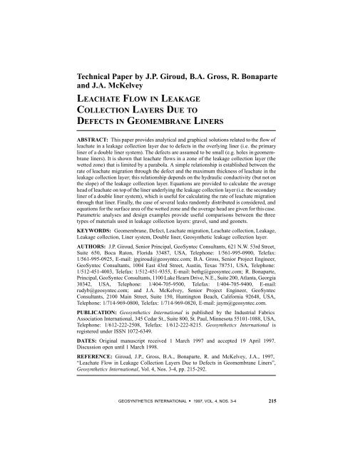
Technical Paper by J.P. Giroud, B.A. Gross, R. Bonaparte 

and J.A. McKelvey 

LEACHATE FLOW IN LEAKAGE 

COLLECTION LAYERS DUE TO 

DEFECTS IN GEOMEMBRANE LINERS 

ABSTRACT: This paper provides analytical and graphical solutions related to the flow of 

leachate in a leakage collection layer due to defects in the overlying liner (i.e. the primary 

liner of a double liner system). The defects are assumed to be small (e.g. holes in geomembrane 

liners). It is shown that leachate flows in a zone of the leakage collection layer (the 

wetted zone) that is limited by a parabola. A simple relationship is established between the 

rate of leachate migration through the defect and the maximum thickness of leachate in the 

leakage collection layer; this relationship depends on the hydraulic conductivity (but not on 

the slope) of the leakage collection layer. Equations are provided to calculate the average 

head of leachate on top of the liner underlying the leakage collection layer (i.e. the secondary 

liner of a double liner system), which is useful for calculating the rate of leachate migration 

through that liner. Finally, the case of several leaks randomly distributed is considered, and 

equations for the surface area of the wetted zone and the average head are given for this case. 

Parametric analyses and design examples provide useful comparisons between the three 

types of materials used in leakage collection layers: gravel, sand and geonets. 

KEYWORDS: Geomembrane, Defect, Leachate migration, Leachate collection, Leakage, 

Leakage collection, Liner system, Double liner, Geosynthetic leakage collection layer. 

AUTHORS: J.P. Giroud, Senior Principal, GeoSyntec Consultants, 621 N.W. 53rd Street, 

Suite 650, Boca Raton, Florida 33487, USA, Telephone: 1/561-995-0900, Telefax: 

1/561-995-0925, E-mail: jpgiroud@geosyntec.com; B.A. Gross, Senior Project Engineer, 

GeoSyntec Consultants, 1004 East 43rd Street, Austin, Texas 78751, USA, Telephone: 

1/512-451-4003, Telefax: 1/512-451-9355, E-mail: bethg@geosyntec.com; R. Bonaparte, 

Principal, GeoSyntec Consultants, 1100 Lake Hearn Drive, N.E., Suite 200, Atlanta, Georgia 

30342, USA, Telephone: 1/404-705-9500, Telefax: 1/404-705-9400, E-mail: 

rudyb@geosyntec.com; and J.A. McKelvey, Senior Project Engineer, GeoSyntec 

Consultants, 2100 Main Street, Suite 150, Huntington Beach, California 92648, USA, 

Telephone: 1/714-969-0800, Telefax: 1/714-969-0820, E-mail: jaym@geosyntec.com. 

PUBLICATION: Geosynthetics International is published by the Industrial Fabrics 

Association International, 345 Cedar St., Suite 800, St. Paul, Minnesota 55101-1088, USA, 

Telephone: 1/612-222-2508, Telefax: 1/612-222-8215. Geosynthetics International is 

registered under ISSN 1072-6349. 

DATES: Original manuscript received 1 March 1997 and accepted 19 April 1997. 

Discussion open until 1 March 1998. 

REFERENCE: Giroud, J.P., Gross, B.A., Bonaparte, R. and McKelvey, J.A., 1997, 

“Leachate Flow in Leakage Collection Layers Due to Defects in Geomembrane Liners”, 

Geosynthetics International, Vol. 4, Nos. 3-4, pp. 215-292. 

GEOSYNTHETICS INTERNATIONAL S 1997, VOL. 4, NOS. 3-4 

215

GIROUD et al. D Leachate Flow in Leakage Collection Layers Due to Geomembrane Defects 

1 INTRODUCTION 

1.1 Leakage Collection Layer 

Many landfills, especially those containing hazardous waste, are lined with a double 

liner system. This paper addresses the design of the drainage layer, called “leakage 

collection layer”, located between the two liners, i.e. the primary liner located above 

and the secondary liner located below the leakage collection layer. The purpose of the 

leakage collection layer is to collect the leachate that migrates (“leaks”) through the 

primary liner and to convey it toward collector pipes. The collector pipes then convey 

the leachate to a sump where it is removed from the landfill. The leakage collection layer 

also allows detection of liquid migrating (“leaking”) through the primary liner, and 

as a result it is also called “leakage detection and collection layer”. It should not be 

called “leak detection layer” since it does not detect individual leaks. 

1.2 Leachate Flow 

1.2.1 Description of the Flow 

To reach the leakage collection layer, leachate first flows through a defect in the primary 

liner (Figure 1a). In this paper the only mechanism of leachate migration through 

the primary liner that is considered is advective flow through defects in the liner. Phenomena 

such as permeation or diffusion of leachate or its constituents through a liner 

are not considered in this paper. 

Leachate flow is governed by the hydraulic gradient. After it has passed through a 

defect in the primary liner, the leachate flows more or less vertically through the leakage 

collection layer upper part, which is unsaturated (Figure 1a). When the leachate reaches 

the saturated part of the leakage collection layer, it flows downgradient, which for a 

small fraction of the leachate consists of first flowing upslope then turning gradually 

to flow downslope with the rest of the leachate (Figure 1b). As a result, the leachate 

flows only in a portion of the leakage collection layer called the wetted zone. The 

boundary of the wetted zone has approximately the shape of a parabola (Figure 1b), 

which will be demonstrated in Section 2.2. 

1.2.2 Definition of the Two Cases, “Not Full” and “Full” 

The case described above and illustrated in Figure 1 is the usual case where the leachate 

phreatic surface in the leakage collection layer is not in contact with the primary 

liner. In this paper, this case is referred to as “the case where the leakage collection layer 

is not full”. The case where the leachate phreatic surface in the leakage collection layer 

is in contact with the primary liner is shown in Figure 2. In this paper, this case is referred 

to as the case where the leakage collection layer is full in a certain area around 

the primary liner defect, or more simply “the case where the leakage collection layer 

is full”. In this paper, both cases will be analyzed: the case where the leakage collection 

layer is not full and the case where the leakage collection layer is full. 

216 GEOSYNTHETICS INTERNATIONAL S 1997, VOL. 4, NOS. 3-4


(a) 

Leachate infiltration 

Waste 

Leachate phreatic 

surface in the 

leachate collection 

layer 

Leachate flow 

in the leachate 

collection 

layer 



leakage 

collection layer 


in the leakage 


Leachate 


Primary liner 

with defect 

Leakage 


Secondary liner 

Small fraction of 

leachate flowing upslope 

(b) 


Boundary of the 

wetted zone 

Wetted zone 

Defect in the 

primary liner 




Figure 1. Leachate flow in the leachate collection layer, through a defect in the primary 

liner, and in the leakage collection layer in the case where the leakage collection layer is not 

filled with leachate: (a) cross section; (b) plan view of the secondary liner. 

1.3 Scope of the Paper 

The paper presents a theoretical analysis of the flow in the leakage collection layer 

resulting from a leak through a defect in the primary liner. The resulting equations make 

it possible to size leakage collection layers. The analysis also provides the size of the 


217


(a) 



leachate collection 

layer 


in the leachate 

collection 

layer 



leakage 


Leachate infiltration 




Waste 

Leachate 



with defect 

Leakage 



(b) 


Boundary of the 

wetted zone 

Wetted zone 

Defect in 

the primary 

liner 




Figure 2. Leachate flow in the leachate collection layer, through a defect in the primary 

liner, and in the leakage collection layer in the case where the leakage collection layer is 

filled with leachate in a certain area around the primary liner defect: (a) cross section; 

(b) plan view of the secondary liner. 

wetted zone and the average head of leachate on top of the secondary liner in the wetted 

zone: this information is necessary to calculate the rate of leakage through the secondary 

liner. The case where the primary liner has several defects is treated; the defects 

are either randomly distributed (“random scenario”) or their location is such that the 

rate of leakage through the secondary liner is maximum (“worst scenario”). Finally, the 



paper provides an approximate value of the time required for steady-state flow conditions 

to exist and the value of the time required for leachate to travel from the higher 

end to the lower end of the leakage collection layer. 

The defects in the primary liner are assumed to be small in all directions, such as holes 

in geomembrane liners. Therefore, the results of the study presented herein are mostly 

applicable to the case where the primary liner is a geomembrane used alone. However, 

the results of the study may also be useful for the case where the primary liner is a composite 

liner consisting of a geomembrane placed on a geosynthetic clay liner (i.e. a bentonite 

layer encapsulated between two layers of geotextile). 

The leakage collection layer considered in the study can be a layer of granular material 

(e.g. sand or gravel) or a layer of geosynthetic drainage material (e.g. geonet or geocomposite 

consisting of a geonet core and two geotextiles). The results of the study are 

particularly useful for the case of relatively thin leakage collection layers, such as those 

consisting of geosynthetic drainage materials. 

2 ASSUMPTIONS 

2.1 General Assumptions 

The following general assumptions are made: 

S The leakage collection layer, the primary liner, and the secondary liner have a uniform 

slope, β. The thickness of the leakage collection layer is t LCL (Figure 3). 

S The leachate collection layer is assumed to be a porous medium. Therefore, the flow 

of leachate is governed by equations for flow in porous media, such as Darcy’s equation 

for the case of laminar flow. Furthermore, the porous medium is assumed to be 

homogeneous, i.e. it does not contain large open spaces such as pipes and channels. 

Therefore, the flow of leachate is not treated using equations for flow in pipes and 

channels. 

S Flow in the leakage collection layer is laminar (i.e. Darcy’s equation is applicable) 

and the leakage collection layer material is characterized by its hydraulic conductiv- 

Q 

t LCL 

β 

Figure 3. 

General assumptions. 


219


ity, k. The laminar flow assumption is applicable to sand and approximately applicable 

to gravel and geonets. Furthermore, it is assumed that the hydraulic conductivity, 

k, of a given leakage collection layer material has a unique value, that is the hydraulic 

conductivity of the saturated material. 

S The leachate is assumed to have the same density and viscosity as water. This assumption 

should be satisfied in the case of all modern landfills due to the generally low 

concentration of chemicals in leachate. As a result, the values of the hydraulic conductivity, 

k, of the leakage collection layer material measured using water are applicable 

to leachate flow. 

S The defects in the primary liner are assumed to have a small dimension in all directions 

of the plane of the geomembrane so that the resulting leaks can be treated as 

point source leaks. Examples of such defects are circular or quasi-circular holes in 

geomembranes with a diameter (or an equivalent diameter) of less than approximately 

10 to 20 mm (i.e. a surface area less than approximately 1 to 3 cm 2 ). Examples of 

defects that are not consistent with the above assumption are defects with a surface 

area larger than approximately 3 cm 2 and defects with a great length such as cracks 

or a relatively long length of open seam in a geomembrane. 

S The rate of leachate migration through a given defect is Q under steady-state flow 

conditions, which are assumed to exist in all cases. 

S It is assumed that flows through various defects do not interfere. In other words, the 

wetted zones related to different defects do not overlap. (Cases where wetted zones 

may overlap are discussed in Section 4.4.5.) 

S Capillarity in the leakage collection layer is not considered (which limits the validity 

of the study by excluding leakage collection layers constructed with fine sands) and 

the secondary liner is assumed to be impermeable (i.e. it is a geomembrane with no 

defects, possibly on a clay layer, but not a clay layer alone). Therefore, all of the leachate 

that passes through defects in the primary liner flows in the leakage collection 

layer. 

Other assumptions will be made as required at various steps in the analysis. 

2.2 AssumptionsSpecific to the Case Where the Leakage Collection Layer is not 

Full 

As mentioned in Section 1.2.2, two cases are discussed in this paper: the case where 

the leakage collection layer is not full and the case where the leakage collection layer 

is full. The former will be the lead case, and results for the case where the leakage 

collection layer is full will then be derived from results for the case where the leakage 

collection layer is not full. 

In the case where the leakage collection layer is not full, the flow rate through the 

considered defects in the primary liner is assumed to be small enough that the maximum 

thickness of leachate in the leakage collection layer is less than the thickness of the leakage 

collection layer. In this case, assumptions regarding the hydraulic gradient and the 

shape of the phreatic surface can be made, as described below. 

As indicated in Section 1.2.1, the leachate that, has passed through a defect in the primary 

liner, first flows more or less vertically through the leakage collection layer upper 



part, which is unsaturated. Then, when the leachate reaches the saturated portion of the 

leakage collection layer, it first flows in all directions (Figure 1). It is therefore logical 

to assume that the leachate phreatic surface in the leakage collection layer is a cone with 

its apex at Point A located vertically beneath the defect in the primary liner (Figure 4). 

Furthermore, for leachate to flow in all directions, the hydraulic gradient must be 

(a) 


Assumed phreatic 

surface 

Actual phreatic 

surface 

Defect 

β 

t LCL 

A 

t o 

β 

D o 

Secondary 

liner 

β 

O 

Horizontal plane 

V 

(b) 

Assumed phreatic 

surface 

β 

D o 

A 

β 

2 D o /tanβ 

P 

O 

Horizontal plane 

Pi 

Figure 4. Assumed phreatic surface in the leakage collection layer in the case where the 

leakage collection layer is not filled with leachate: (a) cross section in a vertical plane along 

the slope and passing through the defect in the primary liner; (b) cross section in a vertical 

plane perpendicular to the plane of the preceding cross section and passing through the 

defect. 


221


approximately the same in all directions. Since the hydraulic gradient is closely related 

to the slope of the phreatic surface, it may then be assumed that the slope of the cone 

generatrices is the same in all directions. The slope of the phreatic surface (i.e. the slope 

of the cone generatrix) in the direction of the slope of the leakage collection layer is 

approximately known: it is close to the slope angle, β, since the flow thickness is small 

compared to the length of the leakage collection layer. Therefore, it is assumed that the 

angle between all generatrices of the cone that form the phreatic surface of leachate and 

a horizontal plane is β (Figure 4). 

From the foregoing discussion, it appears that the wetted zone (Figure 1b) is parabolic 

since the intersection of a cone and a plane parallel to a generatrix of the cone is a parabola. 

However, the actual wetted zone is only approximately parabolic because several 

simplifying assumptions were made, as indicated in Section 2.1 and, above, in Section 

2.2. 

2.3 Assumptions Specific to the Case Where the Leakage Collection Layer is 

Full 

The case where “the leakage collection layer is full” is the case where the flow rate 

through the considered defect in the primary liner is large enough that the thickness of 

leachate in the leakage collection layer is equal to the thickness of the leakage collection 

layer in an area greater than zero around the defect in the primary liner. At the periphery 

of this area, the leachate phreatic surface is in contact with the primary liner. 

As indicated in Section 2.2, the case where the leakage collection layer is not full is 

the lead case. Accordingly, assumptions regarding the hydraulic gradient and the shape 

of the phreatic surface (described in Section 2.2 for the case where the leakage collection 

layer is not full) will be adapted to the case where the leakage collection layer is 

full, as shown in Section 3.2. 

3 RATEOFLEACHATEFLOW 

3.1 Rate of Leachate Flow When the Leakage Collection Layer is not Full 

The leakage collection layer is not full if the following condition is met: 

t 

o 

£ t 

LCL 

(1) 

where: t o = maximum thickness of leachate in the leakage collection layer, which occurs 

at the defect of the primary liner, i.e. at the apex of the phreatic surface (Figure 4a); and 

t LCL = thickness of the leakage collection layer (Figures 3 and 4a). 

In the case where the leakage collection layer is not full, the vertical cross section of 

the flow in a plane passing through the defect and containing the horizontal contour 

lines of the liners (Figure 4b) is a triangle whose surface area is: 

S= 2 /tanb 

D o 

(2) 



where: D o = depth of leachate in the leakage collection layer at the primary liner defect 

(i.e. at the apex of the phreatic surface); and β = angle of the slope of the leakage collection 

layer, which is also the angle of the cone that forms the assumed phreatic surface. 

The leachate depth is measured vertically, whereas the leachate thickness is measured 

perpendicularly to the liners. The following general (and classical) relationship exists 

between the leachate head on top of a liner, h, the leachate depth, D, and the leachate 

thickness, t: 

h = t cosb 

= D cos 

2 b 

(3) 

Therefore, at the apex of the phreatic surface, the following relationship exists between 

the leachate head on top of the secondary liner, h o , the leachate thickness, t o ,and 

the leachate depth, D o : 

h = t cosb 

= D 

o o o 

cos 

2 b 

(4) 

The flow cross section area perpendicular to the flow in the leakage collection layer, 

S F , is the projection of S, hence: 

S 

F 

= 

Scosb 

(5) 

Combining Equations 2, 4 and 5 gives: 

S 

F 

= t 

2 /sinb 

o 

(6) 

Flow in the leakage collection layer is governed by Darcy’s equation: 

Q= 

kiS F 

(7) 

where: Q = steady-state rate of leachate flow in the leakage collection layer, which results 

from a defect in the primary liner and which is, therefore, equal to the rate of leachate 

migration through the defect; and i = hydraulic gradient in the leakage collection 

layer. 

As discussed in Section 2.2, the slope of the leachate phreatic surface in the leakage 

collection layer is extremely close to the liner slope angle β. Therefore, the hydraulic 

gradient is virtually equal to the classical value of the hydraulic gradient for flow parallel 

to a slope, which is: 

i = sin b 

(8) 


2 

Q= 

k t o 

(9) 

hence: 

t 

o 

= 

Q 

k 

(10) 


223


It appears that, when the leakage collection layer is not full, there is an extremely simple 

relationship between the rate of leachate migration through the primary liner defect, 

Q, and the thickness of leachate in the leakage collection layer beneath the defect, t o . 

It is interesting to note that this relationship does not depend on the size of the defect 

in the primary liner or on the slope of the leakage collection layer. 

An approximation that was made to establish Equations 9 and 10 was to assume that 

the downslope flow line from A (i.e. AB in Figure 4a) is parallel to the liner. This assumption 

is close to reality as discussed in Section 2.2. However, the actual flow line 

from A is below Line AB as the flow thickness decreases in the downslope direction, 

as discussed at the end of Section 5.1.2. Therefore, t o should only be regarded as the flow 

thickness at a primary liner defect, and it is the maximum flow thickness. 

Since the simple relationship expressed by Equations 9 and 10 was demonstrated for 

the case when the leakage collection layer is not full, the condition expressed by Equation 

1 must be met for Equations 9 and 10 to be valid. Combining Equations 1 and 10 

gives the following equation, which is another way to express the condition that should 

be met to ensure that the leakage collection layer is not full: 

t 

LCL 

≥ t = 

LCL full 

where t LCLfull is the minimum thickness that a leakage collection layer with a hydraulic 

conductivity k should have to contain, without being full at any location, the leachate 

flow which results from a defect in the primary liner. 

The following equation, derived from Equation 11, is another way to express the condition 

that should be met to ensure that the leakage collection layer is not full: 

Q ≤ Q = kt 

full 

where Q full is the maximum steady-state rate of leachate migration through a defect in 

the primary liner that a leakage collection layer, with a thickness t LCL and a hydraulic 

conductivity k, can accommodate without being filled with leachate. 

It is important to remember that the subscript full corresponds to a minimum thickness 

of the leakage collection layer and to a maximum rate of leachate migration (which is 

also the maximum flow rate in the leakage collection layer). It is noteworthy that the 

minimum thickness of the leakage collection layer, t LCLfull , and the maximum flow rate, 

Q full , which are required to ensure that the leakage collection layer can contain, without 

being full, the flow that results from a defect in the primary liner, do not depend on the 

slope of the leakage collection layer. 

It is not impossible to design a leakage collection layer with a thickness less than the 

value t LCLfull given by Equation 11, i.e. where the flow rate is greater than Q full defined 

by Equation 12. In this case, the leakage collection layer is filled with leachate in a certain 

area around the defect of the primary liner (i.e. “the leachate collection layer is 

full”). This case is discussed in Section 3.2. 

2 

LCL 

Q 

k 

(11) 

(12) 



3.2 Rate of Leachate Flow When the Leachate Collection Layer is Full 

If the thickness of the leakage collection layer is less than t LCLfull expressed by Equation 

11 (or if the rate of leachate migration through a primary liner defect is greater than 

Q full expressed by Equation 12, which is equivalent), the leakage collection layer is 

filled with leachate in a certain area around the defect. Following the approach described 

in Section 2.2, it may then be assumed that the leachate phreatic surface in the 

leakage collection layer is a truncated cone (Figure 5). The virtual apex of the truncated 

cone, Ai, is above the leakage collection layer (i.e. above the primary liner, which is 

the upper boundary of the leakage collection layer). The virtual leachate depth, D o ,and 

the virtual leachate thickness, t o , are related to the actual leachate head, h o , through 

Equation 4, and the virtual leachate thickness t o is greater than the thickness of the leachate 

collection layer: 

t 

o 

> t 

LCL 

(13) 

The surface area of the vertical cross section of the flow in the leakage collection layer 

(Figure 5) is expressed by: 

2 2 

D D D 

o 

b o 

- 

LCLg 

DLCL ( 2 Do - DLCL 

) 

S = - 

= 

(14) 

tan b tan b tan b 

where D LCL is the depth of the leakage collection layer. 

The depth is measured vertically whereas the thickness is measured perpendicularly 

to the slope, hence, in accordance with Equation 3: 

t 

LCL 

= D cosb 

LCL 

(15) 

Using the demonstration presented in Section 2.2, i.e. combining Equations 4, 5, 7, 

8, 14 and 15, gives: 

Q= k t ( 2t - t ) 

LCL o LCL 

(16) 


β 

A 

β 

D LCL 

D o 


Figure 5. Vertical cross section of the assumed phreatic surface in the leakage collection 

layer in the case where the leakage collection layer is filled with leachate in a certain area 

around the primary liner defect. 


225


Knowing (or assuming) the leachate head, h o , on top of the secondary liner vertically 

beneath the primary liner defect, one may derive the virtual leachate thickness, t o ,using 

Equation 4. Then, knowing t o , t LCL and k, one may use Equation 16 to calculate the rate 

of leachate flow through a defect that the leakage collection layer can convey. 

The following equation can be derived from Equation 16: 

t 

o 

F 

HG 

tLCL 

= + 

2 

Q 

kt 

1 

2 

LCL 

I 

KJ 

(17) 

The following equation can be derived from Equations 13 and 16: 

F Q 

tLCL 

= to 

1− 1− 

2 

kt 

HG 

o 

I 

KJ 

(18) 

Equation 18 is valid only if the following condition is met: 

2 

Q ≤ k t o 

(19) 

It should be noted that if t LCL = t o , i.e. if the leakage collection layer is filled with leachate 

at only one point, i.e. at the location of the primary liner defect, Equation 16 is 

equivalent to Equation 9. 

3.3 Parametric Study 

Using the equations presented in Sections 3.1 and 3.2 it is possible to compare the 

flow capacity of different leakage collection layers in case of a defect in the primary 

liner. In Table 1, three different leakage collection layers are compared: 

S a geonet with a thickness of 5 mm and a hydraulic transmissivity resulting in a hydraulic 

conductivity (obtained by dividing the hydraulic transmissivity by the thickness) 

of 1 × 10 -1 m/s; 

S a gravel layer with a thickness of 300 mm and a hydraulic conductivity of 1 × 10 -1 

m/s; and 

S a sand layer with a thickness of 300 mm and a hydraulic conductivity of 1 × 10 -3 m/s. 

The first two leakage collection layers have the same hydraulic conductivity and the 

last two have the same thickness. In the case of the geonet, the virtual leachate thickness, 

t o , considered in Table 1 is greater than, or equal to, the thickness of the leachate 

collection layer, t LCL ; therefore, in all cases considered in Table 1, the geonet is filled 

with leachate over a certain area around the defect (this area being zero for t o = 5 mm). 

In the case of the gravel and sand layers, the leachate thicknesses considered in Table 

1 are less than, or equal to, the thickness of the leakage collection layer; therefore, in 

all cases considered in Table 1, the gravel and sand layer are not filled (or just filled) 

with leachate, and for these two materials the leachate thicknesses, t o ,showninTable 

1 are actual (not virtual) thicknesses. 



Table 1. Rate of leachate flow in three different leachate collection layers resulting from a 

defect in the primary liner. 

Leachate thickness 

(actual or virtual) 

Geonet 

t LCL =5mm 

k =1× 10 -1 m/s 

Leakage collection layer material 

Gravel 

t LCL = 300 mm 

k =1× 10 -1 m/s 

Sand 


k =1× 10 -3 m/s 

t o Q Q Q 

(m) (mm) (m 3 /s) (lpd) (m 3 /s) (lpd) (m 3 /s) (lpd) 

0.005 5 2.5 × 10 -6 216 2.5 × 10 -6 216 2.5 × 10 -8 2.16 

0.01 10 7.5 × 10 -6 648 1.0 × 10 -5 864 1.0 × 10 -7 8.64 

0.05 50 4.75 × 10 -5 4,104 2.5 × 10 -4 21,600 2.5 × 10 -6 216 

0.1 100 9.75 × 10 -5 8,424 1.0 × 10 -3 86,400 1.0 × 10 -5 864 

0.3 300 2.975 × 10 -4 25,704 9.0 × 10 -3 777,600 9.0 × 10 -5 7,776 

Notes: The leachate thickness, t o , can be derived from the leachate head on top of the secondary liner using 

Equation 4. The leachate thickness, t o , isthe actual leachate thickness if t o < t LCL and a virtual leachate thickness 

if t o > t LCL . The tabulated values of the rate of leachate flow, Q, were calculated using Equation 9 when t o < 

t LCL and Equation 16 when t o > t LCL . Units: 1 m 3 /s = 86,400,000 liters per day (lpd). 

It appears from Table 1, that for a given value of t o , i.e. a given value of the head of 

leachate on top of the secondary liner, h o (see Equation 4), the gravel and the geonet 

can convey significantly more leachate than the sand. It is interesting to compare the 

flow rates of Table 1 with rates of leachate migration through defects of geomembranes 

used alone (i.e. not part of a composite liner) calculated using Bernoulli’s equation, 

which is expressed as follows: 

2 2 

Q= 06 . a 2gh = 06 . p( d / 4) 2gh ≈ ( 2/ 3) 

d gh 

prim prim prim 

(20) 

where: a = defect area; d = defect diameter; g = acceleration due to gravity; and h prim 

= head of leachate on top of the primary liner. 

Table 2 gives rates of leachate migration through geomembrane defects calculated 

using Equation 20. It appears that, with the leachate heads that typically exist on the 

primary liners of actively operating landfills (i.e. landfills that are receiving waste), and 

provided that the geomembrane is used alone (i.e. is not part of a composite liner): 

S a small geomembrane defect (e.g. 1 to 2 mm diameter), which may occasionally be 

undetected during construction, results in a rate of leakage on the order of 100 liters 

per day (lpd); 

S a geomembrane defect (e.g. 3 to 5 mm diameter), which may occasionally occur during 

construction phases where defect detection may not be possible (e.g. placement 

of granular leachate collection material on geomembrane), results in a rate of leakage 

on the order of 1000 lpd (1 m 3 /day); and 

S a large geomembrane defect (e.g. 10 mm diameter or more), which may occur under 

special circumstances, results in a rate of leakage of 10,000 lpd (10 m 3 /day) or more. 


227


Table 2. Rate of leachate migration through a defect in a geomembrane primary liner as a 

function of the defect diameter and the head of leachate on top of the primary liner. 

Leachate head on top of the 

Geomembrane primary liner defect diameter, d (mm) 

primary liner, h prim (mm) 1 2 3 5 10 20 50 100 

5 13 51 115 319 1,275 5,101 31,881 127,523 

10 18 72 162 451 1,803 7,214 45,086 180,345 

50 40 161 363 1,008 4,033 16,131 100,816 403,264 

100 57 228 513 1,426 5,703 22,812 142,575 570,301 

300 99 395 889 2,469 9.878 39,512 246,948 987,790 

Note: The tabulated values of the rate of leachate migration, Q, through a geomembrane defect were 

calculated using Bernoulli’s equation (Equation 20) and are expressed in liters per day (lpd). 

Table 1 shows that, in the case of a leachate head on top of the secondary liner on the 

order of 100 mm, which is possible and acceptable in the case of a large leak, the rates 

of leachate flow that can be conveyed by the various leachate collection layers are on 

the following order: gravel, 100,000 lpd; geonet, 10,000 lpd; and sand, 1,000 lpd. 

Therefore, geonets and, to a greater extent, gravel are suitable for all of the defect scenarios 

mentioned above, whereas sand is not. However, it should be noted that, with a 

maximum head on the order of 100 mm, a geonet is full in a certain area around the 

primary liner defect, whereas a gravel leakage collection layer is not. 

If the primary liner is a composite liner (e.g. a geomembrane on a geosynthetic clay 

liner) the rate of leachate migration through a geomembrane defect is several orders of 

magnitude less than through the same defect in a geomembrane used alone. Therefore, 

a geonet leakage collection layer is not likely to be filled with leachate migrating 

through a composite primary liner. 

4 WETTED ZONE 

4.1 Shape of the Wetted Zone 

4.1.1 Equations of the Parabola 

From Section 2.2, it is already known that the wetted zone has the shape of a parabola. 

The equation of the projection of this parabola on a horizontal plane will be provided 

in this section, and any subsequent reference to the wetted zone (e.g. equation, surface 

area) will be related to the projection on a horizontal plane. However, it should be noted 

that the width of the parabola is the same in the actual parabola (on the plane inclined 

at angle β ) and its projection on a horizontal plane. 

Several points of the parabola (Figure 6) are known from Figure 4. Thus, Figure 4a 

and Equation 4 show that the distance between the projection, O, of the flow apex, A, 

and the vertex, V, of the parabola is: 



t o /(sinβ) 

P 

O 

V 

Pi 

t o /(2 sinβ) 

Y 

y 

Defect 

Wetted zone 

x 

X 

x 

W 

Figure 6. 

Projection on a horizontal plane of the parabolic boundary of the wetted zone. 

OV = ( D / 2) / tan b = t / ( 2sin b) 

o 

o 

(21) 

Figure 4b and Equation 4 show that: 

OP = OP ¢ = D / tan b = t / sinb 

o 

o 

(22) 

Since OP and OPi are twice the value of OV, O is the focus of the parabola, and 

t o /(2sinβ ) is the focal distance, hence, from the classical equation of a parabola with 

the origin of axes at the vertex: 

Y 

to 

= X sin b 

2 2 

The origin of axes VX and VY is the vertex of the parabola. The following relationships 

exist between the coordinates, X and Y, in the axes VX and VY, and the coordinates, 

x and y, in the axes Ox and Oy which have their origin at the focus of the parabola: 

(23) 

t o 

X = x + 2sinb 

(24) 


229


Y 

= y 

(25) 

Combining Equations 23, 24 and 25 gives the equation of the parabola in axes Ox and 

Oy as follows: 

y 

2 

2to 

x to 

= + 

2 

sinb 

sin b 

2 

(26) 

Equation 26 can also be written: 

y 

2 

2 

F 

HG 


x 

= 1+ 

2 

2 



t 

o 

I 

KJ 

(27) 

4.1.2 Comment on the Development of the Equations 

It should be noted that the equation of the parabola was obtained with a minimum 

amount of calculations because it was recognized in Section 2.2, using geometric considerations, 

that the curve had to be a parabola. Thus, it was straightforward to establish 

the equation of a parabola passing by three known points, P, Pi and V (Figure 6). If it 

had not been recognized that the curve was a parabola, it would have been necessary 

to use the analytical method to determine the equation of an unknown curve, which consists, 

in this particular case, of determining in polar coordinates the intersection of a 

cone and an inclined plane, and converting the obtained equation into cartesian coordinates. 

The senior author has checked that this lengthy method yields Equation 27. 

4.1.3 Equations for the Case Where the Leakage Collection Layer is not Full 

Combining Equations 10, 23 and 26 gives the following equations for the parabola 

that delimitates the wetted zone in the case where the leakage collection layer is not full: 

2 Q 2 X 

Y = 

k sin b 

(28) 

hence: 

y 

y 

2 

2 

2x Q/ 

k Q 

= + 

2 

sin b k sin b 

F 

HG 

Q x 

1 2 sinb 

= + 

2 

k sin b Q/ 

k 

I 

KJ 

(29) 

(30) 



4.1.4 Equations for the Case Where the Leakage Collection Layer is Full 

Combining Equations 17, 23 and 26 gives the following equations for the parabola 

that delimitates the wetted zone in the case where the leakage collection layer is full 

in a certain area around the primary liner defect: 

hence: 

y 

y 

2 

2 

Y 

F 

HG 

2 

xtLCL 

= 1 + 


F 

HG 

F 

HG 

I 

XtLCL 

= 1 + 


Q 

2 

kt 

LCL 

2 

tLCL 

Q 

= 1+ 

1 

2 2 

4 sin b kt 

LCL 

Q 

2 

kt 

LCL 

I 

KJ 

F 

HG 

2 

tLCL 

+ 1 + 

KJ 

4 sin b 

L 

2 

I 

+ 

KJ N 

M 

Q 

kt 

2 2 

LCL 

t 

LCL 

4 x sinb 

F 

HG 

1 + 

Q 

2 

kt 

LCL 

I 

KJ 

2 

O 

I 

KJ 

Q 

P 

(31) 

(32) 

(33) 

4.2 Width of the Wetted Zone 

4.2.1 Width of the Wetted Zone in the General Case 

The width of the wetted zone depends on the considered location which is defined 

by its horizontal distance X to the vertex, V, of the parabola, or the horizontal distance 

x to the focus, O, of the parabola (Figure 6). 

The width, W, of a parabola defined by an equation of the Y 2 = aX type is given by: 

W 

= 2 Y 

(34) 

Combining Equations 23 and 34 gives: 


X 

W = 2 2 sin b 

(35) 

where X is the horizontal distance between the vertex of the parabola and the location 

where the width of the parabola (i.e. the width of the wetted zone) is evaluated. 



x 

W = 1+ 


sin b t 

o 

(36) 

where x is the horizontal distance between the defect in the primary liner and the location 

where the width of the wetted zone is evaluated. 


231


4.2.2 Width of the Wetted Zone at Special Locations 

The width, W o , of the parabola at the location of the defect in the primary liner is 

given by Equation 36 for x = 0, and is also twice the value of OP given by Equation 22, 

hence: 

W 

o 


= 2 


For a given leachate collection layer whose length along the slope has a horizontal 

projection L, the maximum value of the width of the wetted zone occurs when the defect 

in the primary liner is at the high end of the leakage collection layer slope (Figure 7), 

i.e. when: 

(37) 

x = L 

(38) 

The maximum width of the wetted zone, W max , is then obtained by combining Equations 

36 and 38: 

W 

max 


L 

= 1+ 

2 sinb 

sin b t 

o 

(39) 


Defect 

L 

Maximum 

wetted zone 

A wmax 

W max 

Figure 7. Wetted zone when the defect in the primary liner is at the high end of the leakage 

collection layer slope (truncated parabola). 

Note: The case shown above is identical to the two cases shown in Figure 8 when x = L, x being the 

distance between the primary liner defect and the lower end of the leakage collection layer. 



4.2.3 Width of the Wetted Zone in the Case Where the Leakage Collection Layer is not 

Full 

Combining Equations 10, 35, 36, 37 and 39 gives the following equations for the case 

where the leakage collection layer is not full (t o < t LCL ), i.e. when the condition expressed 

by Equation 11 (or Equation 12, which is equivalent) is met: 

W= 2 ( X /sin b) ( Q/ k) 

32 / 12 / 14 / 

L 

N 

M 

Q 

W = 2 

k 

+ 2 


Wo = 2 


L 

N 

M 

2 Q 

Wmax = + 2 

sin b k 

Q 

k x sin b 

Q 

k 

Q 

k L 

O 

Q 

P 

12 / 


O 

Q 

P 

12 / 

(40) 

(41) 

(42) 

(43) 

4.2.4 Width of the Wetted Zone in the Case Where the Leakage Collection Layer is Full 

Combining Equations 17, 35, 36, 37 and 39 gives the following equations for the case 

where the leakage collection layer is full (t o > t LCL ), i.e. when the condition expressed 

by Equation 11 (or Equation 12, which is equivalent) is not met: 

F 

HG 

L 

N 

M 

XtLCL 

Q 

W = 2 1+ 

2 


kt 

W t Q 

LCL 

= 1+ 

1 

2 


kt 

W 

o 

LCL 

F 

HG 

L 

I 

+ 

KJ N 

M 

F 

HG 

t 

LCL 

LCL 

IO 

KJ 

Q 

P 

12 / 


F Q 

1 + 

2 

kt 

HG 

tLCL 

Q 

= + 

sinb 1 2 

kt 

LCL 

I 

KJ 

LCL 

O 

I 

KJ 

Q 

P 

12 / 

(44) 

(45) 

(46) 


233


W 

max 

F 

HG 

tLCL 

Q 

= 1+ 

1 

2 


kt 

LCL 

L 

I 

+ 

KJ N 

M 

t 

LCL 

4 L sinb 

F 

HG 

Q 

1 + 

2 

kt 

LCL 

O 

I 

KJ 

Q 

P 

12 / 

(47) 

4.2.5 Parametric Study 

Widths of wetted zones calculated using equations given in Section 4.2 are presented 

in Table 3. It appears that the width of the wetted zone increases for increasing rates of 

flow through the geomembrane defect and for decreasing hydraulic conductivities and 

slopes of the leakage collection layer. 

4.3 Surface Area of the Wetted Zone 

4.3.1 Expressions for the Surface Area of the Wetted Zone 

The surface area of a parabola is given by the following equation: 

A=( 23 / ) WX 

(48) 

Table 3. Width of the wetted zone at a 20 m horizontal distance from a defect in the 

geomembrane primary liner for a 2% slope, W 20(2%) , and for a 1V:3H slope, W 20(1/3) . 

Rate of flow 

through the 

geomembrane 

defect 

Geonet 

t LCL =5mm 

k =1× 10 -1 m/s 

Leakage collection layer material 

Gravel 


k =1× 10 -1 m/s 

Sand 


k =1× 10 -3 m/s 

10 lpd 

(1.16 × 10 -7 m 3 /s) 

Not full, t o 

W 20(2%) 

W 20(1/3) 

= 1.1 mm 

= 2.94 m 

= 0.74 m 

Not full, t o 

W 20(2%) 

W 20(1/3) 

= 1.1 mm 

= 2.94 m 

= 0.74 m 

Not full, t o 

W 20(2%) 

W 20(1/3) 

= 11 mm 

= 9.34 m 

= 2.33 m 

100 lpd 

(1.16 × 10 -6 m 3 /s) 

Not full, t o 

W 20(2%) 

W 20(1/3) 

= 3.4 mm 

= 5.23 m 

= 1.31 m 

Not full, t o 

W 20(2%) 

W 20(1/3) 

= 3.4 mm 

= 5.23 m 

= 1.31 m 

Not full, t o 

W 20(2%) 

W 20(1/3) 

= 34 mm 

= 16.84 m 

= 4.15 m 

1,000 lpd 

(1.16 × 10 -5 m 3 /s) 

Full, 

W 20(2%) 

W 20(1/3) 

t o =14mm 

= 10.70 m 

= 2.67 m 

Not full, t o 

W 20(2%) 

W 20(1/3) 

= 11 mm 

= 9.34 m 

= 2.33 m 

Not full, t o 

W 20(2%) 

W 20(1/3) 

= 108 mm 

= 31.24 m 

= 7.41 m 

10,000 lpd 

(1.16 × 10 -4 m 3 /s) 

Full, 

W 20(2%) 

W 20(1/3) 

t o =118mm 

= 32.94 m 

= 7.77 m 

Not full, t o 

W 20(2%) 

W 20(1/3) 

= 34 mm 

= 16.84 m 

= 4.15 m 

Full, t o = 343 mm 

W 20(2%) = 62.28 m 

= 13.29 m 

W 20(1/3) 

Notes: The values of t o were calculated using Equation 10 (when the leakage collection layer is not full) or 

Equation 17 (when the leakage collection layer is full). Values of W 20 were calculated using Equation 36. They 

could have been obtained using Equation 41 (when the leakage collection layer is not full) or Equation 45 

(when the leakage collection layer is full). The leakage collection layer is full when t o > t LCL (Equation 13). 

Units: lpd = liter per day = 1.16 × 10 -8 m 3 /s. 



where: W = width of the base of the parabola; and X = distance between the vertex and 

the base. 

Therefore, from Equations 35 and 48, the surface area of the wetted zone, A w , between 

the vertex, V, and the horizontal line at the distance X from the vertex is: 

A 

w 

= 4 3 


32 / 

X 


(49) 

The surface area of the wetted zone can also be expressed as follows by combining 

Equations 24, 36 and 48: 

A 

w 

F 2 to 

= 

H G I K J 

F 

+ 

3 sin b HG 

x 

1 2 sin b 

t 

o 

I 

KJ 

2 32 / 

However, as shown in Figure 8, Equations 49 and 50 are valid only if the following 

conditions are met: 


L 

2sinb £ 


X L 

2sinb £ £ 

Combining Equations 24 and 52 gives the following alternative expression for the 

condition expressed by Equation 52: 

(50) 

(51) 

(52) 

0 

£ x £ L - 

2 

t o 


(53) 

If the two conditions expressed by Equations 51 and 52 (or 53, which is equivalent) 

are not met, the parabola is truncated (Figure 8). When the parabola is truncated (i.e. 

in the two cases illustrated in Figure 8), the surface area of the wetted zone is obtained 

by subtracting the surface area of the truncated portion from the surface area expressed 

by Equation 49. The resulting equation is: 

A 

w 

4 to 

= X - ( X - L) 


2 32 / 32 / 

(54) 


A 

w 

2 F 

= 

H G 

3 



I LF 

+ 

KJ 1 

NM 

HG 

I 

F 

HG 

2 3/ 2 3/ 

2 

2 x sin b 2( L - x) sinb 

- 1 - 


KJ 


It should be noted that Equations 54 and 55, which give the surface area of the truncated 

wetted zone, are valid under two different sets of conditions: 

S Set 1 (Figure 8a): 

I 

KJ 

O 

QP 

(55) 


235


(a) 

t t o 

< L L < X < L + o 

t L – o < x < L 

2sinβ 

or 

2sinβ 2sinβ 


L 

x 

X 

(b) 

t o 


> L 

t o 


< X < L + or 0 instead of ≤ and ≥). 

Notes: The dot represents the horizontal projection of the location of the primary liner defect and L is the 

horizontal projection of the length of the leakage collection layer. The limit case for x = L can exist for any 

value of t o /(2L sinβ); it is illustrated in Figure 7. 


L 

2sinb £ 

and 

t o 

L £ X £ L + 2sinb 

(57) 

the condition expressed by Equation 57 being equivalent to: 




L - £ x £ L 

2sinb 

(58) 

S Set 2 (Figure 8b): 


L 

2sinb ≥ 

(59) 

and 



£ X £ L + 



(60) 

the condition expressed by Equation 60 being equivalent to: 

0 ≤ x ≤ 

L 

(61) 

4.3.2 Maximum Surface Area of the Wetted Zone 

For a given leachate collection layer whose length along the slope has a horizontal 

projection L, the maximum value of the surface area of the wetted zone, A wmax , occurs 

when the defect in the primary liner is at the high end of the leakage collection layer 

slope (Figure 7), i.e. when x = L (Equation 38). 

In this case, the parabola is truncated (Figure 7) and the equation for the surface area 

of the wetted zone is obtained by combining Equations 38 and 55, hence: 

A 

wmax 

F 2 to 

= 

H G I L 

K J F 

+ 


NM 

HG 

2 32 

L 

1 2 sin b 

1 

t 

o 

/ 

I O 

- 

KJ QP 

The same equation would have been obtained by combining Equations 24, 38 and 54. 

(A table and a graph for calculating A wmax will be provided in Section 4.4.3.) 

4.3.3 Summary of the Cases 

Regarding the geometry of the wetted zone, there are two major cases depending on 

whether the parabola is complete (Figures 1, 2 and 6) or truncated. When the parabola 

is truncated, there are two cases, as illustrated in Figure 8, with a limit case illustrated 

in Figure 7. Therefore, there is a total of four cases, one case of a complete parabola 

and three cases of truncated parabolas. (These cases will be considered again in Section 

5.1.1.) 

4.3.4 Actual and Projected Surface Areas 

It should be remembered that, as indicated at the beginning of Section 4.1.1, the projection 

of the wetted zone on a horizontal plane is considered in the analysis, which is 

(62) 


237


more convenient for theoretical analyses as well as practical applications. However, if 

the actual surface area of the wetted zone, A w actual , were needed, it could be derived from 

the surface area given above using the following equation: 

A = A /cosb 

(63) 

wactual 

The various widths of the wetted zone are unchanged in the projection. 

4.3.5 Surface Area of the Wetted Zone in the Case Where the Leakage Collection Layer 

is not Full 

Combining Equation 10 with Equations 49 to 62 gives the following equations for the 

case where the leakage collection layer is not full (t o < t LCL ), i.e. when the condition expressed 


S When the parabola is complete, i.e. when the following conditions are met: 

w 

Q/ 

k 

L 

2 sinb £ 

(64) 

and 

Q/ 

k 

X L 

2 sinb £ £ 

(65) 

the latter being equivalent to 

0 

£ x £ L - 

2 

Q/ 

k 


(66) 

the surface area of the wetted zone is expressed by 

A = ( 4/ 3)( 2/sin b) ( Q/ k) 

X 

w 

F 

HG 

12 / 14 / 32 / 

2Q 

x 

Aw = 1+ 


2 

3k 

sin b Q/ 

k 

I 

KJ 

32 / 

(67) 

(68) 

S When the parabola is truncated, the surface area of the wetted zone is expressed by: 

Aw = ( 4/ 3)( 2/sin b) ( Q/ k) X - ( X - L) 

L 

MF 

NHG 

12 / 14 / 32 / 32 / 

2 Q 2 x sinb 

2( L - x) sinb 

Aw = 1 + 

- 1 - 

2 

3 k sin b M Q/ 

kKJ Q/ 

k 

I 

F 

HG 

I 

KJ 

32 / 32 / 

O 

QP 

(69) 

(70) 



Equations 69 and 70 are valid under two different sets of conditions. The first set is: 

Q/ 

k 

L 

2 sinb £ 

(71) 

and 

L £ X £ L + 

the latter condition being equivalent to 

Q/ 

k 


(72) 

Q/ 

k 

L - £ x £ L 


(73) 

The second set of conditions is: 

Q/ 

k 

L 

2 sinb ≥ 

(74) 

and 

Q/ 

k 

Q/ 

k 

£ X £ L + 



(75) 

the later condition being equivalent to 

0 < x < 

L 

(76) 

S In the limit case between the case where the parabola is truncated and the case where 

it is not, Equations 64 to 76 become: 

Q/ 

k 

L X 

2 sinb = = 

x = 0 

A = 8 w 

L 

2 / 3 

(77) 

(78) 

(79) 

S The surface area of the maximum wetted zone (Figure 7) is derived from Equation 

70 for x = L, which gives: 

L 

F 

NM 

HG 

32 / 

I 

- 

KJ 

2Q 

L 

Awmax = 1+ 


1 

2 

3k 

sin b Q/ 

k 

O 

QP 

(80) 


239


4.3.6 Surface Area of the Wetted Zone in the Case Where the Leakage Collection Layer 

is Full 

Combining Equation 17 with Equations 49 to 62 gives the following equations for the 

case where the leakage collection layer is full (t o > t LCL ), i.e. when the condition expressed 

by Equation 11 (or Equation 12, which is equivalent) is not met: 

S When the parabola is complete, i.e. when the following conditions are met: 

and 

tLCL 


tLCL 


the latter being equivalent to 

F 

HG 

F 

HG 

Q 

kt 

1 + 

2 

LCL 

Q 

kt 

1 + 

2 

LCL 

I 

I 

£ 

KJ 

tLCL 

0 £ x £ L - + 


L 

£ X £ L 

KJ 

F 

HG 

Q 

1 

2 

ktLCL 

the surface area of the wetted zone is expressed by 

A 

w 

L 

M 

A 

w 

L 

N 

M 

F 

HG 

L 

N 

M 

4 32 / tLCL 

= X 1 + 


F 

IO 

2 

1 tLCL 

Q 

= 1+ 

N HG 

ktLCLKJ 

Q 

P 1+ 

2 


t 

Q 

2 

kt 

LCL 

LCL 

I 

KJ 

IO 

KJ 

Q 

P 

12 / 


F Q 

1 + 

2 

kt 

S When the parabola is truncated, the surface area of the wetted zone is expressed by: 

A 

w 

L 

F 

A 

w 

F 

HG 

4 tLCL 

= + 


IO 

R 

L 

S| 

M 

N 

M 

T| 

2 

1 tLCL 

Q 

= + 

N 

M 1 

HG 

ktLCLKJ 

Q 

P 1+ 

2 


| M 

t 

Q 

kt 

1 

2 

LCL 

LCL 

I 

HG 

LCL 

X - ( X - L) 

KJ 

32 / 32 / 

O 

I 

KJ 

Q 

P 

32 / 

4 x sin b 

4( L - x) sinb 

- 1 - 

F Q I 

Q 

+ P 

M 

F 

1 

tLCL 

1 + 

2 

2 

kt 

kt 

HG 

LCL 

O 

P 

KJ 

Q 

L 

M 

N 

HG 

LCL 

O 

I 

KJ 

Q 

P 

32 / 32 / 

Equations 86 and 87 are valid under two different sets of conditions. The first set is: 

U 

V| 

W| 

(81) 

(82) 

(83) 

(84) 

(85) 

(86) 

(87) 



and 

tLCL 


F 

HG 

Q 

kt 

1 + 

2 

LCL 

F 

HG 

I 

£ 

KJ 

tLCL 

L £ X £ L + + 



The second set of conditions is: 

and 

tLCL 


F 

HG 

F 

HG 

tLCL 

L - + 


1 + 

tLCL 


Q 

kt 

I 

F 

HG 


Q 

k 

1 

2 

LCL 

Q 

kt 

1 + 

2 

LCL 

L 

Q 

kt 

1 

2 

LCL 

I 

I 

KJ 

£ x £ L 

KJ 

I 

≥ 

KJ 

L 

F 

HG 

tLCL 

£ X £ L + 1 + 

KJ 


Q 

kt 

2 2 

LCL 

LCL 

0 ≤ x ≤ 

L 

I 

KJ 

(88) 

(89) 

(90) 

(91) 

(92) 

(93) 

S In the limit case between the case where the parabola is truncated and the case where 

it is not, Equations 81 to 93 become: 

tLCL 


F 

HG 

Q 

kt 

1 + 

2 

LCL 

x = 0 

I 

Aw = 8 L 

2 / 3 

= L = X 

KJ 

S The surface area of the maximum wetted zone (Figure 7) is derived from Equation 

87 for x = L, which gives: 

A 

wmax 

L 

F 

IO 

R 

L 

S| 

M 

N 

M 

T| 

2 

1 tLCL 

Q 

= + 

N 

M 1 

HG 

ktLCLKJ 

Q 

P 1+ 

2 


| M 

t 

LCL 


F Q 

1 + 

2 

kt 

HG 

LCL 

O 

I 

KJ 

Q 

P 

32 / 

U 

V| 

W| 

- 1 

(94) 

(95) 

(96) 

(97) 


241


4.4 Wetted Fraction 

4.4.1 Scope of Section 4.4 

To calculate the rate of leakage through the secondary liner, it is useful to know what 

fraction of the total surface area of the secondary liner is wetted and what is the average 

head of leachate over this fraction of the secondary liner. The wetted fraction is determined 

in Sections 4.4.3 and 4.4.4, and the average head will be determined in Sections 

5.1 and 5.2. 

In the preceding sections, only one defect in the primary liner was considered. This 

is no longer the case in Section 4.4 because the wetted fraction depends on the number 

of defects per unit area. In Section 4.4, two scenarios of defect location will be considered: 

a scenario where the defects are located to give the maximum wetted fraction, and 

a scenario where the defects are at random. 

In Section 4.4, a leakage collection layer whose length in the direction of the flow 

has a horizontal projection L, and whose width in the direction perpendicular is B, is 

considered (Figure 9). The projected surface area of this leakage collection layer is 

therefore: 

A 

LCL = 

LB 

(98) 

4.4.2 Definitions 

Wetted Fraction. The wetted fraction, R w , is defined as the ratio between the surface 

area of the total wetted zone and the surface area of the leakage collection layer: 

R 

w 

n 

N 

= 

∑ 

n 

= = 1 

A 

A 

LCL 

w 

(99) 

As shown by the numerator of the fraction, the surface area of the total wetted zone 

is the sum of the surface areas of the wetted zones that correspond to every defect in 

the primary liner, the number of defects being N. 

Defect Frequency. The frequency of defects, F, in the primary liner (i.e. the liner overlying 

the leakage collection layer) is defined as the ratio of the total number of defects, 

N, in the liner and the surface area of the liner, which is equal to the surface area of the 

leakage collection layer: 

F = 

N 

A LCL 

(100) 

In typical design calculations the frequency of the defects in the primary liner, F, is 

assumed to be known. For example, if there are four defects per hectare (10,000 m 2 ), 

F = 4/(10,000 m 2 ) = (4/10,000) m -2 = (1/2,500) m -2 =4× 10 -4 m -2 . 



(a) 

B 

L 

(b) 

W max 

B 

L 

Figure 9. Leakage collection layer zones wetted by leachate migrating through several 

defects in the primary liner, assuming no overlapping of wetted zones: (a) worst 

scenario where all the defects are located at the high end of the leachate collection layer 

slope; (b) random scenario where the defects are randomly distributed. 

Notes: L is the horizontal projection of the length of the leakage collection layer in the direction of the flow, 

and B is the width of the leakage collection layer. The dots represent the horizontal projection of the locations 

of the primary liner defects. 

Scenarios. Two defect location scenarios will be considered: (i) the worst scenario 

where all of the defects are at the high end of the leakage collection layer slope (Figure 

9a); and (ii) the random scenario where the defects are randomly distributed (Figure 

9b). In both scenarios it is assumed that the frequency of defects is small enough that 

the wetted zones related to each individual defect do not overlap. 


243


4.4.3 Wetted Fraction in the Worst Scenario 

In the worst scenario (Figure 9a), the leachate flow through each defect generates a 

wetted zone whose surface area is A wmax (Figure 7) given by Equation 62 (which is 

equivalent to Equation 97 or 80 depending on whether the leakage collection layer is 

full or not, respectively). Therefore, the surface area of the total wetted zone for the scenario 

where all the defects are at the high end of the leakage collection layer slope is 

expressed as follows, if all of the leaks are assumed to be equal, which is generally the 

case in design: 

n= 

N 

∑ Aw 

= 

n = 1 

N A 

wmax 

(101) 

Combining Equations 99 and 101 with R w = R w worst gives: 

R 

w worst 

NA 

= 

A 

wmax 

LCL 

(102) 


R 

w worst 

= FA 

w max 

(103) 

Combining Equations 62 and 103 gives the following equation for the wetted fraction 

in the worst scenario: 

R 

wworst 

2F to 


1 


t 

= 

F H G 

I LF 

+ 

KJ NM 

HG 

o 

/ 

I 

- 

KJ 

2 3 2 

O 

QP 

1 

(104) 

Combining Equations 80 and 103 gives the following equation for the worst scenario 

when the leakage collection layer is not full (t o < t LCL ), i.e. when the condition expressed 


2 FQ 

32 / 

R L 

wworst= 1+ 2L k Q -1O 

2 d sin b / i 

(105) 

3k 


NM 

Combining Equations 97 and 103 gives the following equation for the worst scenario 

when the leakage collection layer is full in a certain area around the primary liner defect 

(t o > t LCL ), i.e. when the condition expressed by Equation 11 (or Equation 12, which is 

equivalent) is not met: 

R 

wworst 

L 

F 

IO 

R 

L 

S| 

M 

N 

M 

T| 

2 

F tLCL 

Q 

= + 

N 

M 1 

HG 

ktLCLKJ 

Q 

P 1+ 

2 


| M 

t 

LCL 


F Q 

1 + 

2 

kt 

HG 

LCL 

QP 

O 

I 

KJ 

Q 

P 

32 / 

- 1 

U 

V| 

W| 

(106) 



For practical calculations, it is convenient to use the following dimensionless expression: 

R 

w worst 

=lworst 

F L 

2 

(107) 

where λ worst is a dimensionless factor derived from Equation 104 and defined as follows: 

L 

F 

NM 

HG 

l = 2 2 

worst 

m 1 

3 

+ 2 

m 

32 / 

I 

- 

KJ 

where μ is a dimensionless parameter defined as follows: 

O 

QP 

1 

(108) 

m = 


L sin b 

(109) 

Values of λ worst calculated using Equation 108 are given in Table 4 and Figure 10 as a 

function of the dimensionless parameter μ. It should be noted that λ worst can also be used 

to calculate A wmax using the following equation derived from Equations 103 and 107: 

A 

wmax 

=lworst 

L 

2 

(110) 

Combining Equations 10 and 109 gives μ for the case when the leakage collection 

layer is not full: 

m = 

Q/ 

k 

L sinb 

(111) 

Combining Equations 17 and 109 gives μ for the case when the leakage collection 

layer is full: 

F 

HG 

tLCL 

m = + 

2 Lsinb 

4.4.4 Wetted Fraction in the Random Scenario 

Q 

kt 

1 

2 

LCL 

I 

KJ 

(112) 

In the random scenario, the surface area of the total wetted zone is given by the following 

equation, which is similar to Equation 101 for the worst scenario: 

n= 

N 

∑ 

n = 1 

A 

w 

= N A 

w rand 

(113) 

where A w rand is the average surface area of the wetted zones generated by leachate flow 

through defects located at random, assuming that all of the leaks are equal, which is a 

typical assumption in design. 

Combining Equations 99 and 113 with R w = R w rand gives: 


245


Table 4. Values of λ worst , λ rand , λ worst /λ rand , Crit(R wworst ) and Crit(R wrand ) as a function of the 

dimensionless parameter μ. 

μ λ worst λ rand λ worst /λ rand Crit (R w worst ) Crit (R w rand ) 

1 × 10 -4 1.886 × 10 -2 7.543 × 10 -3 2.500 0.667 0.267 

2 × 10 -4 2.667 × 10 -2 1.067 × 10 -2 2.500 0.667 0.267 

3 × 10 -4 3.267 × 10 -2 1.307 × 10 -2 2.500 0.667 0.267 

5 × 10 -4 4.218 × 10 -2 1.688 × 10 -2 2.499 0.667 0.267 

1 × 10 -3 5.967 × 10 -2 2.388 × 10 -2 2.499 0.667 0.267 

2 × 10 -3 8.445 × 10 -2 3.382 × 10 -2 2.497 0.667 0.267 

3 × 10 -3 1.035 × 10 -1 4.147 × 10 -2 2.496 0.668 0.267 

5 × 10 -3 1.338 × 10 -1 5.367 × 10 -2 2.493 0.668 0.268 

1 × 10 -2 1.899 × 10 -1 7.637 × 10 -2 2.487 0.670 0.269 

2 × 10 -2 2.704 × 10 -1 1.094 × 10 -1 2.473 0.673 0.272 

3 × 10 -2 3.334 × 10 -1 1.356 × 10 -1 2.459 0.675 0.275 

5 × 10 -2 4.359 × 10 -1 1.794 × 10 -1 2.430 0.681 0.280 

1 × 10 -1 6.349 × 10 -1 2.692 × 10 -1 2.359 0.693 0.294 

2 × 10 -1 9.462 × 10 -1 4.259 × 10 -1 2.222 0.713 0.321 

3 × 10 -1 1.214 5.787 × 10 -1 2.097 0.731 0.348 

5 × 10 -1 1.697 8.984 × 10 -1 1.889 0.759 0.402 

1 2.797 1.812 1.544 0.808 0.523 

2 4.876 3.901 1.250 0.862 0.690 

3 6.910 5.941 1.163 0.892 0.767 

5 1.094 × 10 1 9.966 1.098 0.925 0.842 

1 × 10 1 2.097 × 10 1 1.998 × 10 1 1.049 0.957 0.912 

2 × 10 1 4.098 × 10 1 3.999 × 10 1 1.025 0.977 0.953 

3 × 10 1 6.099 × 10 1 5.999 × 10 1 1.017 0.984 0.968 

5 × 10 1 1.010 × 10 2 1.000 × 10 2 1.010 0.990 0.981 

1 × 10 2 2.010 × 10 2 2.000 × 10 2 1.005 0.995 0.990 

2 × 10 2 4.010 × 10 2 4.000 × 10 2 1.002 0.998 0.995 

3 × 10 2 6.010 × 10 2 6.000 × 10 2 1.002 0.998 0.997 

5 × 10 2 1.001 × 10 3 1.000 × 10 3 1.001 0.999 0.998 

1 × 10 3 2.001 × 10 3 2.000 × 10 3 1.001 1.000 0.999 

2 × 10 3 4.001 × 10 3 4.000 × 10 3 1.000 1.000 1.000 

3 × 10 3 6.001 × 10 3 6.000 × 10 3 1.000 1.000 1.000 

5 × 10 3 1.000 × 10 4 1.000 × 10 4 1.000 1.000 1.000 

Notes: The dimensionless parameter μ is defined by Equation 109. The following equations were used to 

calculate the tabulated values: λ worst , Equation 108; λ rand , Equation 123 for μ ≤ 2 and Equation 127 for μ ≥ 2; 

Crit(R w worst ), Equation 136; and Crit(R w rand ), Equation 138 for μ ≤ 2 and Equation 140 for μ ≥ 2. It is 

important to note that the tabulated values are valid only if the wetted areas related to various defects in the 

primary liner do not overlap. Values of λ worst and λ rand are also presented in Figure 10, and values of 

Crit(R w worst )andCrit(R w rand ) in Figure 12. 



100 

10 

Dimensionless factor, λ 

1 

10 -1 

λ worst 

λ rand 

(114) 

10 -2 

10 -3 10 -4 10 -3 10 -2 10 -1 1 10 

Dimensionless parameter, μ 

Figure 10. Dimensionless factor λ used to calculate the wetted fraction. 

Notes: λ worst was calculated using Equation 108, and λ rand using Equation 123 for μ ≤ 2 and Equation 127 

for μ ≥ 2; μ is defined by Equation 109. Values of λ worst and λ rand are also presented in Table 4. 

R 

w rand 

= 

N A 

A 

w rand 

LCL 


R 

wrand 

= FA 

wrand 

(115) 

The average surface area of the wetted zones generated by leachate flow through defects 

located at a random distance from the bottom end of the leachate collection layer 

slope is given by the following classical equation used to average functions: 


247


A 

wrand 

1 L 

= 

Lz 

A x wd 

o 

(116) 


A 

wrand 

1 

= 

L 

z 

L + to 

/( 2 sin b ) 



A 

w 

dX 

(117) 

Equations for A w , and therefore integrations, are simpler with X than with x. Therefore, 

Equation 117 will be used instead of Equation 116. 

Two cases must be considered for integration of Equation 117. The first case is defined 

by t o /(2 sinβ) ≤ L (i.e. Equation 51). Combining Equations 51 and 109 gives the 

following condition for the first case of integration: 

m£2 

(118) 

In this case, there are two different expressions for A w depending on X: Equation 49 

(complete parabola) if X meets the condition expressed by Equation 52; and Equation 

54 (truncated parabola) if X meets the condition defined by Equation 57. Therefore, if 

μ ≤ 2, Equation 117 can be written as follows: 

A 

wrand 

L + to 


z z L 

L 

= 1 Aw1 

dX 

+ 

1 

L to 

/( 2 sin b ) L 

A 

w2 

dX 

(119) 

where A w1 is the value of A w expressed by Equation 49 and A w2 is the value of A w expressed 

by Equation 54. 

Integration of Equation 119 gives: 

A 

w rand 

2 

15 L 

= 

F H G 



I LF 

+ 

KJ 1 

NM 

HG 

2 L sin b 

t 

o 

/ 

I 

- 

KJ 

3 5 2 

2 

O 

QP 

(120) 

Combining Equations 115 and 120 gives the following expression for the average 

wetted fraction in the random scenario: 

R 

w rand 

2 F 

15 L 

= 

F H G 



I LF 

+ 

KJ 1 

NM 

HG 

2 L sin b 

t 

o 

/ 

I 

- 

KJ 

3 5 2 

2 

O 

QP 

(121) 

For practical calculations, it is convenient to use the following dimensionless expression: 

R 

w rand 

=lrand 

F L 

where λ rand is a dimensionless factor derived from Equation 121 and defined by: 

2 

(122) 



L 

F 

NM 

HG 

2 3 2 

lrand = m 1 + 

15 m 

52 / 

I 

- 

KJ 

O 

QP 

2 ( for m £ 2) 

(123) 

where μ is a dimensionless parameter defined by Equation 109. 

The second case for integration of Equation 117 is defined by t o /(2 sinβ ) ≥ L (i.e. 

Equation 59). Combining Equations 59 and 109 gives the following condition for the 

second case of integration: 

m≥2 

(124) 

In this case, integration of Equation 117 is performed using the expression of A w given 

by Equation 54, hence: 

A 

w rand 

2 

15 L 

= 

F H G 



I LF 

+ 

KJ 1 

NM 

HG 


R 

w rand 

2 F 

15 L 

= 

F H G 



I 

F 

HG 



+ 1 - 


KJ 


I 

- 

KJ 

3 5/ 2 5/ 

2 

I LF 

+ 

KJ 1 

NM 

HG 


L 

F 

NM 

HG 

I 

F 

HG 



+ 1 - 


KJ 


I 

- 

KJ 

3 5/ 2 5/ 

2 

2 3 2 2 

lrand = m 1 + + 1 - 

15 mKJ m 

I 

F 

HG 

I 

- 

KJ 

52 / 52 / 

O 

QP 

2 ( for m ≥ 2) 

2 

2 

O 

QP 

O 

QP 

(125) 

(126) 

(127) 

where μ is a dimensionless parameter defined by Equations 109, 111 and 112. 

It is important to note that λ rand is given by Equation 123 when μ ≤ 2, and Equation 

127 when μ ≥ 2. Values of λ rand , calculated using Equation 123 for μ ≤ 2 and Equation 

127 for μ ≥ 2, are given in Table 4 and Figure 10 as a function of the dimensionless 

parameter μ. It should be noted that λ rand can be used to calculate A w rand using the following 

equation derived from Equations 115 and 122: 

A 

w rand 

=lrand 

L 

2 

(128) 

Combining Equation 10 with Equations 121 and 126, respectively, gives the following 

values of R w rand for the case where the leakage collection layer is not full (t o ≤ t LCL ), 

i.e. the case where the condition expressed by Equation 11 (or Equation 12, which is 

equivalent) is met: 

S If μ ≤ 2(whereμ is defined by Equation 111) 

L 

F 

NM 

HG 

32 / 

2 F ( Q/ k) 


Rwrand = 1 + 

3 

15 L sin b Q/ 

k 

52 / 

I 

- 

KJ 

2 

O 

QP 

(129) 


249


S If μ ≥ 2(whereμ is defined by Equation 111) 

L 

MF 

NHG 

32 / 

2 F ( Q/ k) 



Rwrand = 1 + 

+ 1 - 

3 

15 L sin b M Q/ 

kKJ Q/ 

k 

I 

52 / 

F 

HG 

I 

KJ - 

2 

O 

QP 

(130) 

Combining Equation 17 with Equations 121 and 126, respectively, gives the following 

values of R w rand for the case where the leakage collection layer is full (t o > t LCL ), i.e. 

the case where the condition expressed by Equation 11 (or Equation 12, which is equivalent) 

is not met: 

S If μ ≤ 2(whereμ is defined by Equation 112) 

R 

w rand 

L 

F 

IO 

R 

L 

S| 

M 

N 

M 

T| 

3 

F tLCL 

Q 

= + 

L N 

M 1 

HG 

ktLCLKJ 

Q 

P 1+ 

2 


| M 

t 

S If μ ≥ 2(whereμ is defined by Equation 112) 

R 

w rand 

L 

F 

IO 

R 

L 

S| 

M 

N 

M 

T| 

3 

F tLCL 

Q 

= + 

L N 

M 1 

HG 

ktLCLKJ 

Q 

P 1+ 

2 


| M 

t 

LCL 


F 

HG 

Q 

1 + 

2 

kt 

LCL 

LCL 

O 

I 

KJ 

Q 

P 


F Q 

1 + 

2 

kt 

HG 

L 

N 

M 

+ 1 - 

t 

LCL 

LCL 

O 

I 

KJ 

Q 

P 

52 / 


F 

HG 

Q 

1 + 

2 

kt 

- 2 

LCL 

U 

V| 

W| 

O 

I 

KJ 

Q 

P 

52 / 52 / 

(131) 

- 2 

U 

V| 

W| 

(132) 

4.4.5 Critical Values of the Wetted Fraction in the Worst Scenario and the Random 

Scenario 

In Section 4.4, so far, it has been assumed that the wetted zones related to the various 

geomembrane defects do not overlap. The critical value of R w worst ,Crit(R w worst ), is the 

maximum value that R w worst can have without overlapping of the wetted zones related 

to the various individual primary liner defects. This occurs when the parabolic wetted 

zones shown in Figure 9a are in contact at the low end of the leachate collection layer 

slope (Figure 11). This situation occurs when: 

W = max 

B / N 


F = 

1 

LW max 

(133) 

(134) 



L 

W max 

B 

Figure 11. Configuration of the wetted zones for the maximum value of the worst scenario 

wetted fraction. 

Note: In this particular figure, the number of defects is N = 3. The dots represent the horizontal projection 

of the locations of the primary liner defects. 

Combining Equations 39, 104 and 134, and calling Crit(R w worst ) the value of R w worst 

thus obtained, give: 

L 

F 

NM 

HG 




Crit( Rwworst) 

= 1 + - 1 + 

3L 



KJ 


I 

F 

HG 

I 

KJ 

-12 

/ 

O 

QP 

(135) 

Combining Equations 109 and 135 gives the following expression for Crit(R w worst ): 

L 

F 

NM 

HG 

m 

Crit( R wworst 

) = 1 + 

3 

I 

F 

HG 

2 

- 1 + 

mKJ m 

I 

KJ 

- / 

2 12 

O 

QP 

(136) 

where μ is a dimensionless parameter defined by Equation 109. 

Values of Crit(R w worst ) are given in Table 4 and Figure 12. The two extreme values of 

Crit(R w worst ) can be explained as follows considering the truncation of the parabolic 

wetted zone defined in Figure 7: 

S When μ is very small, t o is small (according to Equation 109) and the parabolas in 

Figure 11 are hardly truncated. According to Equation 48, full parabolas occupy 2/3 

of the rectangular area in Figure 11, hence the lower value of 2/3 for Crit(R w worst )in 

Figure 12. 

S When μ is very large, t o is large (according to Equation 109) and the parabolas in Figure 

11 are truncated to the point that they are quasi-rectangular. Therefore, the wetted 


251


1.0 

Critical value of R w (dimensionless) 

0.8 

0.6 

0.4 

0.2 

Crit (R wworst ) 

Crit (R wrand ) 

0 

10 -3 10 -2 10 -1 1 10 100 1000 

Dimensionless parameter, μ 

Figure 12. Maximum values of the wetted fractions without overlapping of wetted zones 

in the worst scenario, R wworst , and in the random scenario, R wrand . 

Notes: Crit (R w worst ) was calculated using Equation 136, and Crit (R w rand ) using Equation 138 for μ ≤ 2and 

Equation 140 for μ ≥ 2; μ is defined by Equation 109. Values of Crit (R w worst )andCrit(R w rand )arealso 

presented in Table 4. 

zone occupies the entire leakage collection layer area in Figure 11, hence the upper 

valueof1forCrit(R w worst ) in Figure 12. 

Also represented in Figure 12 is the critical value of R w rand ,Crit(R w rand ), which is the 

maximum value that R w rand can have without overlapping of the wetted zones related 

to the various individual primary liner defects. Selecting the value of the frequency F 

to be used in the calculation of Crit(R w rand ) is not easy. For the sake of consistency with 

the calculation of Crit(R w worst ), the same frequency (i.e. the frequency given by Equation 

134) is used. Accordingly, combining Equations 39, 121 and 134 gives the following 

value of Crit (R w rand )forμ ≤ 2: 

Crit ( R ) 

w rand 

1 F 

= 

H G 

15 



I LF 

+ 

KJ 1 

NM 

HG 


I 

2 2 -1/ 

2 

F 

HG 



- 2 1+ 


KJ 


I 

KJ 

O 

QP 

(137) 



L 

F 

NM 

HG 

2 

m 

Crit ( R w rand 

) = 1 + 

15 

I 

F 

HG 

I 

KJ 

2 -1/ 

2 

2 

2 

- 2 1+ 

mKJ m 

O 

QP 

(138) 

Combining Equations 126 and 134 gives the following value of Crit(R w rand )for 

μ ≥ 2: 

Crit ( R 

wrand 

) 

1 F 

= 

H G 

15 

t 


I 

KJ 

2 

F 

HG 

52 / 52 / 



1 + 

+ 1 - 

t KJ 

t 


1 + 

t 

o o o 

I 

F 

HG 

o 

I 

- 

KJ 

2 

(139) 


F 

HG 

52 / 52 / 

2 2 

1 + + 1 - 

2 

m m 

Crit ( R wrand 

KJ 

m 

) = 

12 / 

15 F 2I 

1 + 

m 

I 

HG 

F 

HG 

KJ 

I 

- 

KJ 

2 

(140) 

If, in the design of a leakage collection layer, Equation 107 gives a value of R w worst 

greater than Crit(R w worst ) and/or Equation 122 gives a value of R w rand greater than Crit(R w 

rand), this means that wetted zones related to different defects overlap. If this happens, 

the equations presented earlier in Section 4.4 are no longer valid. In this case, the design 

(in particular the leachate head calculation) should be done by assuming that the entire 

leakage collection layer area is wetted, i.e. R w = 1. This is further discussed in Section 

5.2.4. 

It should be recognized that even if the wetted fraction, R w , is small (i.e. smaller, or 

even much smaller, than Crit(R w rand ) given by Table 4 or Figure 12) there is always a 

possibility that the wetted zones related to two different defects in the primary liner will 

overlap. For example, if, in a large primary liner, there are only two small defects generating 

a small rate of leachate migration, the two wetted zones will overlap if the two 

defects are close to each other. Therefore, the design engineer can always elect to ignore 

the values of R w rand and R w worst calculated as indicated above (i.e. assuming no wetted 

zone overlapping if R w rand


S primary liner defect frequency from 1 to 300 defects per hectare: 10 -4 m -2 < F


5 LEACHATE HEAD AND TIME REQUIRED FOR STEADY-STATE 

FLOW CONDITIONS 

5.1 Leachate Head on Top of the Secondary Liner Due to One Defect in the 

Primary Liner 

5.1.1 Method Used to Calculate the Head and Thickness of Leachate 

To calculate the rate of leakage through the secondary liner, it is necessary to know 

the head of leachate on top of the secondary liner in the wetted zone. The leachate head 

is related to the leachate thickness through Equation 3. It is important to note that Equation 

3 is valid whether t is an actual leachate thickness (case where the leakage collection 

layer is not full) or a virtual leachate thickness (case where the leakage collection 

layer is full in a certain area around the primary liner defect). 

In Section 5.1, the average leachate thickness in the wetted zone, t avg , will be calculated 

in the case where only one defect in the primary liner is considered. The average 

head of leachate on top of the secondary liner, h avg , can then be calculated using the 

following equation derived from Equation 3: 

h = t cosb 

(141) 

avg 

avg 

The average leachate thickness in the wetted zone can be calculated as follows: 

t 

avg 

= 

V 

A 

w actual 

(142) 

where: V = volume of leakage collection layer that contains leachate; and A w actual =surface 

area of the actual wetted zone (whereas the surface areas noted A w given in Section 

4.3 are the surface areas of the projection of the wetted zone on a horizontal plane; see 

Section 4.3.3). 

It should be noted that V is the volume of leakage collection layer that contains leachate, 

not the volume of leachate. Since leachate only occupies the pores of the leakage 

collection layer, the volume of leachate is: 

V 

leachate = 

n V 

(143) 

where n is the porosity of the leakage collection layer material. 

From Equations 63 and 142, the average thickness of leachate over the wetted zone is: 

t 

avg 

V 

= 

A / cosb 

w 

(144) 

Expressions of A w are given in Section 4.3 for all relevant cases. Therefore, only V 

needs to be calculated at this point. As pointed out in Section 4.3.3, four cases were considered 

in Section 4.3 for the derivation of expressions for A w (the surface area of the 

wetted zone). The same four cases must be considered for the calculation of V. These 

four cases are illustrated in Figure 13. However, whereas for A w analytical expressions 


255


(a) 

Case I μ ≤ 2, 0 ≤ x ≤ L(1 − μ 2 ) 

(b) 

Case II μ ≤ 2, L(1 − μ 2 ) < x < L 

L 

L 

x 

(c) 

Case III μ ≥ 2 

(i.e. arrow greater than L ) 

0


S the case where the defect in the primary liner is located at the high end of the leakage 

collection layer (x = L), regardless of μ (Case IV, Figure 13d). 

Furthermore, an interpolation method will be provided for the Case II (Figure 13b), 

which is defined by Equation 145 (μ ≤ 2) and the following equation derived from 

Equations 58 and 109: 

F m 

L 1 - x L 

(147) 

2 

HG I K J £ £ 

In summary: (i) solutions are provided for μ ≤ 2 (analytical solution for Cases I and 

IV, and interpolation method for Case II); and (ii) no solution will be provided for μ > 

2 (Case III, Figure 13c), with the exception of the solution for Case IV, which does not 

depend on μ. 

The reason no analytical solution is proposed for two cases (Cases II and III in Figure 

13) is that volume calculations are extremely complex. The considered volume is the 

cone formed by the leachate phreatic surface and truncated by three planes: the plane 

of the secondary liner, and two vertical planes located at the high end and the low end 

of the leakage collection layer slope. (However, in Case I, the phreatic surface does not 

meet the vertical plane located at the high end of the leakage collection layer slope; 

therefore, in this case, the phreatic surface is truncated only by two planes, the plane 

of the secondary liner and the vertical plane located at the low end of the leakage collection 

layer slope.) The intersection of the leachate phreatic surface with the secondary 

liner plane is a parabola, as extensively discussed in Section 4, whereas the intersections 

of the phreatic surface with vertical planes are hyperbolas. 

The volume to be calculated can be decomposed into two volumes: the volume of the 

leakage collection layer containing leachate downstream of the defect (x >0);andthe 

volume of the leakage collection layer containing leachate upstream of the defect (x < 

0). A simple expression (in spite of the hyperbolic truncation at the low end of the slope) 

can be obtained for the downstream volume using Darcy’s equation as shown in Section 

5.1.2. However, the hyperbolic truncation makes the calculation of the upstream volume 

quasi-inextricable. (The senior author has obtained the equation of the hyperbolic 

intersection at the high end of the slope and has found that the integration of the hyperbola 

to obtain the volume of the cone could be done analytically but would require 

lengthy calculations that would be beyond the scope of this paper.) The only two cases 

where the upstream volume is simple are Cases I and IV (Figure 13): in Case I, the volume 

is that of a cone whose base and height are known; and, in Case IV, the volume is 

zero. In Case II, an interpolation method will be proposed, and, in Case III, no solution 

will be proposed; however, Case III is rare since μ is rarely greater than 2 as discussed 

in Section 4.5. 

5.1.2 Leachate Thickness in Case I 

In Case I (Figure 13a), the parabola is not truncated. The volume of the leakage 

collection layer containing leachate (above the parabolic wetted zone) can be decomposed 

into two volumes, as explained in Section 5.1.1: the volume located downstream 

of the defect, and the volume located upstream of the defect. 


257


Instead of using an extremely long integration, the downstream volume can be calculated 

using Darcy’s equation as follows: 

v= 

ki 

(148) 

where v is the apparent leachate flow velocity along the slope. 

Since the hydraulic gradient, i, has been assumed to be constant along the slope (as 

indicated by Equation 8), and since the hydraulic conductivity of the leakage collection 

layer material, k, is a constant, the apparent leachate flow velocity, v, is a constant. Since 

the leakage rate, Q , is constant (as steady-state flow conditions were assumed) and the 

apparent leachate flow velocity, v, is constant (as mentioned above), the leachate flow 

cross section area perpendicular to the flow direction is constant along the slope for x 

≥ 0. Therefore, the value of the leachate flow cross section area for x ≥ 0 is equal to 

the value it has for x = 0, i.e. beneath the defect in the primary liner. This value (S F )is 

given by Equation 6 for the case where the leakage collection layer is not full. 

Since the leachate flow cross section is constant for x ≥ 0, the volume of the leakage 

collection layer that contains leachate in the portion of the wetted zone where the flow 

is downslope (i.e. the portion of the parabolic area for x ≥ 0) is as follows: 

V1 = SF 

x /cosb 

(149) 


V 

1 

t 2 

x o 

/cosb 

= 


(150) 

Then, the upstream volume (i.e. the volume of the leakage collection layer that contains 

leachate in the portion of the parabolic wetted zone comprised between axes Oy 

and VY in Figure 6) is calculated as follows using the classical equation for the volume 

of a cone: 

V 

= ( 1/ 3)( t )( 2/ 3)( OV/ cos b )( PP¢ 

) 

2 o 

(151) 

hence, from Figure 6: 

3 

F to to to 

V2= to 

H G 

I 2 2 

( 1/ 3)( )( 2/ 3) 

2 

2sinb cos b sin b 9sin b cos b 

KJ F H G I K J = 

(152) 

From Equations 150 and 152, the total volume of the leakage collection layer that 

contains leachate in the wetted zone in Case I (Figure 13a) is: 

xt 

2 o 

2t 

3 

o 

V = + 

(153) 

2 

sinbcosb 9sin b cos b 


t 

avg 

3( x sin b + 2to 

/ 9) 

= 

32 

21 [ + ( 2x 

sin b )/ t ] / 

o 

(154) 



The above calculations are valid whether t o is actual or virtual. If the leakage collection 

layer is filled with leachate in a certain area around the primary liner defect, t o is 

the virtual leachate thickness in the leakage collection layer at the location of the primary 

liner defect. The fact that virtual leachate thicknesses are considered is not a problem 

since leakage through the secondary liner is governed by the leachate head on top of 

the secondary liner, and the relationship between head and thickness is the same regardless 

whether the leachate thickness is the actual thickness or a virtual thickness. 

Combining Equations 10 and 154 gives the following equation for the case where the 

leakage collection layer is not full: 

t 

avg 

= 

3 

2 

Q 

k 

( 2/ 9) + xsin b k / Q 

32 / 

1+ 

2xsin b k / Q 

d 

i 

(155) 


leakage collection layer is full: 

t 

avg 

F 

HG 

Q 

( 1/ 6) tLCL 

1+ 

+ 3/ 2 x sin 

2 

ktLCLKJ = 

L 

N 

M 

1 + 

t 

LCL 

I 


F Q 

1 + 

2 

kt 

HG 

LCL 

b g b 

32 / 

O 

I 

KJ 

Q 

P 

(156) 

Finally, it should be noted that since the cross sectional area of the flow is constant 

for x ≥ 0 (as noted earlier in Section 5.1.2) and since the width of the parabola increases 

as the distance x from the primary liner defect increases (Figure 6), the thickness of leachate 

flow decreases as x increases (x ≥ 0). Therefore the actual leachate phreatic surface 

is below line AB in Figure 4a. However, the impact of the difference between line 

AB and the actual phreatic surface on the hydraulic gradient is negligible because the 

leachate thickness is very small compared to the length of the leakage collection layer. 

5.1.3 Leachate Thickness in Case IV 

If the defect is at the high end of the leakage collection layer slope (Figures 7 and 13d), 

the volume of the leakage collection layer that contains leachate in the wetted zone, 

V max , is given by Equation 153 with x = L , and with the last term equal to zero, since 

this last term is the volume of the truncated part. Therefore: 

V 

max 

2 

Lto 

= 


cosb 

(157) 

In accordance with Equation 144, the average leachate thickness, t avg L , is given in 

this case by: 


259


t 

avg L 

= 

A 

wmax 

Vmax 

/cosb 

(158) 

It should be noted that the notation used for the average leachate thickness is t avg L (for 

x = L), and not t avg max , since a large wetted zone leads to a relatively small value (not 

a maximum value) of t avg . 


t = ( 3/ 2) Lsinb 

avg L 

(159) 

( + 32 

1 2Lsin b / t ) / - 1 


leakage collection layer is not full: 

t 

avg L 

= 

( 3/ 2) Lsinb 

32 / 

1+ 2Lsin b k / Q) 

-1 

d 

o 

i 

(160) 


leakage collection layer is full: 

t 

avg L 

= 

L 

N 

M 

1 + 

t 

LCL 

( 3/ 2) L sinb 


F Q 

1 + 

2 

kt 

HG 

LCL 

O 

I 

KJ 

Q 

P 

32 / 

- 1 

(161) 

5.1.4 Leachate Thickness in Case II 

Case II (Figure 13b) is a case that may frequently occur. Since it is not easy to develop 

an analytical solution for this case for the reasons indicated in Section 5.1.1, an interpolation 

method is proposed. 

The limit situation between Cases I and II (Figure 13) is illustrated in Figure 14a. This 

situation occurs when: 


F mI x = L - = L 1 - K J 

(162) 

2 sinb 2 

HG 



5 

- 

3 to 


18 

tavg lim 

= 

32 / 

2 F 2 L sinbI 

t 

HG 

o 

KJ 

(163) 



(a) 

μ


t 

avg II 

t 

o 

tavg lim 

t 

ª a + ( 1 - a) 

t 

t 

o 

avg L 

o 

(166) 

where t avg lim is defined by Equation 164, t avg L by Equation 165, and α by: 

a = 

t 

o 

L - x 2 ( L - x) sinb 

= 

/( 2 sin b) 

t 

o 

(167) 

The dimensionless parameter α is related to the location of the primary liner defect 

as illustrated in Figure 15. It should be noted that Equations 166 and 167 are valid only 

if: 

0 £ a £ 1 

(168) 

This condition is met if the conditions required for Case II to exist are met (Figure 13b). 

Numerical values of Equation 166 are given in Table 5. It should be noted that both 

Equations 164 and 165 approach the same limit when μ approaches 0: 

Lim 

F 

HG 

t 

avg lim 

t 

o 

I 

F t 

= Lim 

KJ H G 

t 

avg L 

m = 0 o m = 0 

I 

3 m 

= = 

KJ 

4 2 

0. 

530 

m 

(169) 

In Table 5, one may expect to see the value t avg /t o = 1/3, which is the classical value 

for the average height of a cone (see Equation 151), since the phreatic surface has been 

assumed to be a cone (see Figures 1 and 4). In fact, the value t avg /t o = 1/3 appears only 

once in Table 5: for α =1andμ = 2. This case is illustrated in Figure 14b. This is the 

only case where the truncation does not affect the cone volume. In all other cases, the 

phreatic surface is a truncated cone and the average height of a truncated cone is not 

equal to one third of its total height. 


α 

0.0 

0.2 

0.4 

0.6 

0.8 

1.0 


x 

Primary liner defect 

L 

Figure 15. Definition of the dimensionless parameter α used in Equation 166 and in 

Table 5. 

Note: In the case illustrated above, α = 0.43. 



Table 5. Values of t avg II /t o for Case II defined in Figure 13b. 

μ 

α 

0 0.2 0.4 0.6 0.8 1.0 

1.0 × 10 -4 0.005 0.005 0.005 0.005 0.005 0.005 

1.0 × 10 -3 0.017 0.017 0.017 0.017 0.017 0.017 

2, Case II does not exist. Values in the column for α = 0 are identical to values of t avg worst /t o in Table 6, 

except that in Table 6 there is no limitation at μ =2. 

5.1.5 Leachate Thickness in Case III 

As indicated in Section 5.1.1, no solution is proposed for the average leachate thickness 

(and head) in Case III (Figure 13). However, it should be noted that Case III is rare 

because μ rarely exceeds 2 as discussed in Section 4.5. 


263


5.2 Leachate Head on Top of the Secondary Liner Due to Several Defects in the 

Primary Liner 

5.2.1 Scope of Section 5.2 

The size of the wetted zone in the case where there are several defects in the primary 

liner was discussed in Section 4.4. In this case, the wetted zone consists of several parabolic 

wetted zones, each of these parabolic zones being related to a primary liner defect. 

When the frequency of defects (i.e. the number of defects per unit area) is small, the 

probability for the various parabolic wetted zones to overlap is small and it may be assumed 

that they do not overlap. In contrast, when the frequency of defects is high, the 

parabolic wetted zones will likely overlap. 

In Section 4.4, the wetted fraction was defined as the ratio between the surface area 

of the total wetted zone and the surface area of the leakage collection layer. The wetted 

fraction was calculated in the worst scenario, i.e. the scenario where all primary liner 

defects are at the high end of the leakage collection layer slope, and in the random scenario, 

i.e. the scenario where primary liner defects are distributed at random. 

In Section 5.2, the worst scenario and the random scenario will be considered to calculate 

the average leachate thickness in the wetted zone. The cases where the wetted 

zones, related to different defects in the primary liner, do not overlap are considered first 

(Sections 5.2.2 and 5.2.3) followed by the case where the wetted zones overlap (Section 

5.2.4). Finally, comments on the influence of primary liner defect frequency on average 

leachate thickness will be presented in Section 5.2.5. 

5.2.2 Average Leachate Thickness in the Worst Scenario With no Overlap 

In the worst scenario (defined in Section 4.4.2), if the primary liner defect frequency 

is small enough that the parabolic wetted zones do not overlap, all of the parabolic zones 

are identical (Figure 9a). Therefore, the average leachate head in the total wetted zone 

in the worst scenario, t avg worst , is identical to the average leachate head in any of the parabolic 

zones, hence: 

t 

avg worst 


t 

avg worst 


t 

avg worst 

t 

o 

= t 

avg L 


= 

32 

( 1+ 2 L sin b / t ) / -1 

3 

= 

2 

2 m 1+ 

m 

L 

F 

NM 

HG 

o 

32 / 

I 

- 

KJ 

O 

QP 

1 

(170) 

(171) 

(172) 



where μ is defined by Equation 109. Values of t avg worst /t o as a function of μ are given 

in Table 6. 

Table 6. Values of t avg worst /t o , t avg rand /t o , t avg rand /t avg worst ,andt avg rand λ rand /(t avg worst λ worst ). 

μ 

t avgworst 

t o 

t avgrand 

t o 

t avgrand 

t avgworst 

t avgrand λ rand 

t avgworst λ worst 

1 × 10 -4 0.0053 0.0072 1.3572 0.5429 

2 × 10 -4 0.0075 0.0102 1.3572 0.5429 

3 × 10 -4 0.0092 0.0125 1.3571 0.5429 

5 × 10 -4 0.0119 0.0161 1.3571 0.5430 

1 × 10 -3 0.0168 0.0227 1.3570 0.5431 

2 × 10 -3 0.0237 0.0321 1.3567 0.5432 

3 × 10 -3 0.0290 0.0393 1.3564 0.5434 

5 × 10 -3 0.0374 0.0507 1.3558 0.5438 

1 × 10 -2 0.0527 0.0713 1.3543 0.5446 

2 × 10 -2 0.0740 0.0999 1.3512 0.5464 

3 × 10 -2 0.0900 0.1213 1.3478 0.5482 

5 × 10 -2 0.1147 0.1538 1.3408 0.5517 

1 × 10 -1 0.1575 0.2083 1.3225 0.5507 

2 × 10 -1 0.2114 0.2717 1.2855 0.5787 

3 × 10 -1 0.2472 0.3091 1.2507 0.5963 

5 × 10 -1 0.2947 0.3505 1.1892 0.6297 

6 × 10 -1 0.3117 0.3623 1.1624 0.6451 

7 × 10 -1 0.3259 0.3708 1.1379 0.6594 

8 × 10 -1 0.3380 0.3769 1.1152 0.6728 

9 × 10 -1 0.3484 0.3812 1.0942 0.6849 

1.000 0.3575 0.3841 1.0746 0.6959 

1.0696 0.3632 0.3855 1.0616 0.7029 

2 0.4102 0.43 1.04 0.83 

3 0.4342 0.45 1.03 0.89 

5 0.4570 0.47 1.02 0.93 

1 × 10 1 0.4769 0.48 1.01 0.96 

2 × 10 1 0.4880 0.49 1.01 0.98 

3 × 10 1 0.4919 0.49 1.00 0.98 

5 × 10 1 0.4951 0.50 1.00 0.99 

1 × 10 2 0.4975 0.50 1.00 0.99 

2 × 10 2 0.4988 0.50 1.00 1.00 

3 × 10 2 0.4992 0.50 1.00 1.00 

5 × 10 2 0.4995 0.50 1.00 1.00 

∞ 0.5000 0.5000 1.0000 1.0000 

Notes: The tabulated values were calculated using the following equations: t avg worst /t o , Equation 172; and 

t avg rand /t o , Equation 189 for 0 < μ ≤ 1.0696. Values of t avg rand /t avg worst for μ > 1.0696 were interpolated 

graphically between 1.0616 and 1.000. Values of t avg rand /t o for μ > 1.0696 were then derived. Values of t avg rand 

λ rand /(t avg worst λ worst ) were calculated using Equation 192 for μ ≤ 1.0696 and were calculated numerically 

(using values of λ rand and λ worst from Table 3) for μ > 1.0696. The dimensionless parameter μ is defined by 

Equation 108. It is important to note that the tabulated values are valid only if the wetted areas related to various 

defects in the primary liner do not overlap. 


265


Comparing Equations 108 and 172 shows that: 

t 

avg worst 

t 

o 

m 

= 

l 

worst 

(173) 

Equation 173 could have been established in two steps. First, combining Equations 

109 and 157 gives: 

V cosb = L 2 m t 

max 

o 

(174) 

Then, combining Equations 110, 158, 170 and 174 gives Equation 173. 

If the leakage collection layer is not full (i.e. if the condition expressed by Equation 

11 is met), Equation 10 can be combined with Equation 171, which gives: 

t 

avg worst 

= 

d 


32 / 

1+ 2 L sin b k / Q -1 

i 

(175) 

If the leakage collection layer is filled with leachate in a certain area around the primary 

liner defect (i.e. if the condition expressed by Equation 11 is not met), Equations 

17 and 171 can be combined to give: 

t 

avg worst 

= 

L 

N 

M 

1 + 

t 

LCL 



F Q 

1 + 

2 

kt 

HG 

LCL 

O 

I 

KJ 

Q 

P 

32 / 

- 1 

(176) 

Another expression for t avg worst can be obtained by combining Equations 105 and 171: 

t 

avg worst 

FLt 

= 

sin b R 

2 

o 

wworst 

(177) 

In the case where the leakage collection layer is not full, combining Equations 10 and 

177 gives: 

t 

avg worst 

= 

FLQ 

k sinb R 

wworst 

(178) 

5.2.3 Average Leachate Thickness in the Random Scenario With no Overlap 

In the random scenario, the size of the wetted zone is known from Section 4.4.4. However, 

contrary to the worst scenario where all parabolic zones are equal (Figure 9a), in 

the random scenario, the parabolic zones are different (Figure 9b). To calculate the average 

leachate thickness without undertaking complex integrations, it is necessary to 



determine the “average parabolic zone” in the random scenario. This can be done as 

follows. 

The “average parabolic zone” in the random scenario is defined by the horizontal distance 

x rand between the primary liner defect and the low end of the leakage collection 

layer slope which is such that the wetted zone surface area calculated using x rand is equal 

to A w rand : 

A A 

(179) 

w ( x = xrand 

) 

= 

wrand 

Considering all of the cases discussed in Section 4.4, Equation 179 has an explicit 

solution only if the following conditions are met: 


L 

(180) 

2sinb £ (181) 

t 

0 £ x £ L - o 



X L 

2sinb £ £ 

(182) 


L 

F 

NM 

HG 

53 / 

xrand m 

= 

23 / 

1 + 

L 10 2 

d 

i 

2 

m 

52 / 

I 

- 

KJ 

where x rand is defined by Equation 179 and μ is defined by Equation 109. 


L 

F 

NM 

HG 

53 / 

Xrand m 

= 

23 / 

1 + 

L 10 2 

d 

i 

2 

m 

2 

O 

QP 

52 / 

I 

- 

KJ 

23 / 

2 

O 

QP 

- 

23 / 

m 

2 

(183) 

(184) 

where X rand is the horizontal distance between the vertex of the parabolic zone and the 

low end of the leakage collection layer slope in the random scenario. 

Values of x rand /L and X rand /L are given in Table 7. It appears that the condition expressed 

by Equation 181 (or Equation 182 which is equivalent) is met only for: 

From Equation 153: 

0 £ m £ 10696 . 

(185) 

V 

rand 

2 3 

xrand to 2 to 

= + 

2 

sinb cosb 9 sin b cosb 

(186) 

where V rand is the volume of the leakage collection layer that contains leachate in the 

random scenario. 


267


Table 7. 

Values of x rand /L and X rand /L. 

μ x rand /L X rand /L 

1 × 10 -4 0.543 0.543 

1 × 10 -3 0.543 0.543 

1 × 10 -2 0.542 0.547 

1 × 10 -1 0.538 0.588 

5 × 10 -1 0.519 0.769 

0.6 0.512 0.812 

0.7 0.504 0.854 

0.8 0.495 0.895 

0.9 0.485 0.935 

1.0 0.474 0.974 

1.0696 0.465 1.000 

Notes: The tabulated values were calculated using the following equations: x rand /L, Equation 183; X rand /L, 

Equation 184. The dimensionless parameter μ is defined by Equation 109. 

From Equation 144: 

t 

avg rand 

= 

A 

Vrand 

/cosb 

w rand 

(187) 

where t avg rand is the average thickness of leachate in the wetted zone of the leakage 

collection layer in the case where the defects in the primary liner are distributed at random 

(random scenario). 


b5 / 3g + b15 / 2gbxrand 

/ togsinb L sinb 

tavg rand 

= 

52 / 

F 2 L sinbI 

(188) 

1 + 

2 

t 


t 

avg rand 

t 

o 

HG 

o 

KJ - 

( 5 / 3) + 15 /( 2m) xrand 

/ L 

= 

52 / 

L 

MF 

2I 

O 

m 1 + 2P 

m 

NM 

HG 

KJ - 

QP 

(189) 

where μ is defined by Equation 109 and x rand /L is given by Equation 183. 

Values of t avg rand /t o as a function of μ, calculated using Equation 189, are given in Table 

6for0≤ μ ≤ 1.0696. 

If the leakage collection layer is not full (i.e. if the condition expressed by Equation 

11 is met), Equations 10 and 188 can be combined to give: 



t 

avg rand 

= 

b 

g 

( 5 / 3) + 15 / 2 x sin b k / Q L sinb 

d 

rand 

52 / 

1+ 2 L sin b k / Q - 2 

i 

(190) 

where x rand is given by Equation 183. 

If the leakage collection layer is filled with leachate in a certain area around the primary 

liner defect (i.e. if the condition expressed by Equation 11 is not met), Equations 

17 and 188 can be combined to give: 

t 

avg rand 

= 

L 

N 

M 

( 5/ 3) 

+ 

t 

L 

N 

M 

1 + 

t 

LCL 

15 xrand 


F Q 

1 + 

2 

kt 

LCL 

HG 


F Q 

1 + 

2 

kt 

HG 

LCL 

O 

I 

KJ 

Q 

P 

52 / 

O 

I 

KJ 

Q 

P 

LCL 


- 2 

(191) 

where x rand is given by Equation 183. 

It should be remembered that Equations 188 to 191 are valid only for μ ≤ 1.0696. 

Values of t avg rand /t o given in Table 6 for μ > 1.0696 were obtained as follows. 

If μ is large, the wetted fractions R w worst and R w rand converge (see Equations 107 and 

122) since λ worst and λ rand tend to become equal when μ is large (see Table 4). The wetted 

zones being the same, the average leachate thickness must be the same and, therefore, 

t avg rand /t avg worst must tend toward one when μ tends toward infinity. Table 6 shows that 

t avg rand /t avg worst is equal to 1.0616 for μ = 1.0696. Therefore, between μ = 1.0696 and 

μ = ∞, t avg rand /t avg worst varies only between 1.0616 and 1.0. Interpolation of t avg rand /t avg worst 

was done graphically between μ = 1.0696 and μ = 100 (where t avg rand and t avg worst become 

virtually equal) following the trend of the curve for values of μ smaller than 1.0696. The 

values of t avg rand /t avg worst thus obtained are given in Table 6. Values of t avg rand /t o were then 

derived from the values of t avg worst /t o and the values of t avg rand /t avg worst . 

Table 6 shows that the average thickness of leachate is between 0 and 33% greater 

in the random scenario than in the worst scenario. However, it should be remembered 

that the average thickness has been calculated over the wetted zone (there is no leachate 

outside the wetted zone) and the wetted zone is between 0 and 150% greater in the worst 

scenario than in the random scenario, as shown in Table 4. Therefore, there is more leachate 

in the leakage collection layer in the worst scenario than in the random scenario. 

The ratio between the amount of leachate in the leakage collection layer in the random 

scenario and the worst scenario is expressed by the following equation derived from 

Equations 123, 173, 183 and 189: 


269


t 

t 

avg rand 

avg worst 

l 

l 

rand 

worst 

L 

F 

NM 

HG 

53 / 

2 m xrand 

m 2 

= + = 

23 / 

1+ 

9 L 10 2 m 

d 

i 

52 / 

I 

- 

KJ 

2 

O 

QP 

23 / 

5m 

- 

18 

(192) 

Equation 192 is valid only for μ ≤ 1.0696. Values calculated using Equation 192 are 

given in Table 6. Values of t avg rand λ rand /(t avg worst λ worst ) given in Table 6 for μ > 1.0696 were 

calculated from numerical values of λ worst /λ rand given in Table 4 and numerical values 

of t avg rand /t avg worst given in Table 6. 

5.2.4 Average Leachate Thickness When Wetted Zones Overlap 

The values of the average leachate thickness given in Sections 5.2.2 and 5.2.3 are valid 

only if there is no overlapping of different wetted zones, i.e. if, as shown in Section 

4.4.5: 

R ≤ Crit ( R ) 

(193) 

wworst 

w worst 

R 

wrand 

≤ Crit ( R ) 

wrand 

(194) 

If the conditions expressed by Equations 193 and 194 are not satisfied, there is overlapping 

between adjacent wetted zones. In this case, the best approach, from a practical 

standpoint, is to assume that the entire area of the leakage collection layer is wetted. 

Again, the worst scenario and the random scenario are considered. These two scenarios 

are defined in Section 4.4.2. 

Worst Scenario. In the worst scenario all of the primary liner defects are located at 

the higher end of the leakage collection layer slope. Since the wetted zones have been 

assumed to overlap, it is approximately correct to consider that the entire leakage 

collection layer area is wetted. As a result, the leachate thickness is approximately uniform 

over the entire leakage collection layer area provided that the defects are uniformly 

distributed at the high end of the leakage collection layer slope. The average leachate 

thickness is then derived using the classical Darcy’s equation, resulting in: 

t 

avg worst 

= 

NQ 

kiB 

(195) 

where: N = total number of defects in the primary liner; Q = rate of leachate migration 

through one defect of the primary liner, all defects being assumed identical and subjected 

to the same leachate head over the entire surface area of the primary liner; k = 

hydraulic conductivity of the leakage collection layer material; i = hydraulic gradient 

in the leakage collection layer; and B = width of the leakage collection layer. 


t 

avg worst 

= 

NQ 

kBsinb 

(196) 




t 

avg worst 

= 

FLQ 

k sinb 

(197) 

Equations 195 to 197 are valid only if the leakage collection layer is not full, i.e. if 

the condition expressed by Equation 11 (or Equation 12 which is equivalent) is met. The 

case where the leakage collection layer is full over its entire surface area is complex: 

(i) Equations 16 to 18, which where established for the case where the leakage collection 

layer is full in a limited area around the primary liner defect, are not applicable; 

and (ii) assuming that the virtual thickness of leachate is a constant (t avg ) over the entire 

area of the leakage collection layer allows Darcy’s equation to be written as follows: 

NQ 

= kBt LCL 


(198) 

which shows that there is no relationship between Q and t avg .Inotherwords,t avg is then 

indeterminate. Therefore, no solution is proposed for the average leachate head (and 

virtual thickness) for the case where the leakage collection layer is filled with leachate. 

Random Scenario. In the random scenario, the primary liner defects are distributed 

at random. In the case where there are enough defects to assume that the entire leakage 

collection layer area is wetted, the design of a leakage collection layer becomes similar 

to the design of a leachate collection layer subjected to a uniform rate of leachate generation. 

As shown by Giroud and Houlihan (1995), in most practical cases, an average 

value of the leachate thickness is : 

t Â Q/( L B) 

avg 

= (199) 

L 2 k sinb 

With the notations used in this paper, Equation 199 becomes: 

NQ 

tavg rand 

= 2 kB sinb 


FLQ 

t = avg rand 

2 k sinb 

(200) 

(201) 

Comparing Equations 197 and 200 shows that the average leachate thickness is twice 

greater in the worst scenario than in the random scenario. (It should be remembered that 

it has been assumed that, in both cases, the entire surface area of the leakage collection 

layer is wetted.) 

Equations 199 to 201 are valid only if the leakage collection layer is not full, i.e. if 

the condition is expressed by Equation 11 (or Equation 12 which is equivalent) is met. 

Also, for the reasons indicated after Equation 197, no solution is proposed for the case 

where the leakage collection layer is full. 


271


5.2.5 Influence of Primary Liner Defect Frequency on Average Leachate Thickness 

An important difference between Sections 5.2.2 and 5.2.3 on one hand, and Section 

5.2.4 on the other hand should be noted. Equations for t avg worst and t avg rand do not depend 

on the defect frequency, F, in Sections 5.2.2 and 5.2.3, whereas they depend on F in 

Section 5.2.4. The reason for that is the following: 

S In Sections 5.2.2 and 5.2.3, the wetted zones, that correspond to various defects in 

the primary liner, do not overlap. The average leachate thickness is the same in any 

of these individual wetted zones and it is calculated for any of them. Consequently, 

the average leachate thickness does not depend on the frequency of defects. However, 

the frequency of defects governs the wetted fraction (i.e. the ratio between the total 

surface area of all wetted zones and the surface area of the leakage collection layer). 

S In Section 5.2.4, it is assumed that the entire surface area of the leakage collection 

layer is wetted. In other words, it is assumed that the wetted fraction is equal to one. 

Therefore, the average leachate thickness is a function of all of the defects in the primary 

liner and, consequently, is a function of the defect frequency. 

It is important to note that, when the wetted fraction exceeds the critical value (Section 

4.4.5), the design engineer must assume that the individual wetted zones (i.e. the 

wetted zones that correspond to the individual defects in the primary liner) overlap and 

must use the equations given in Section 5.2.4 to calculate the average leachate thickness. 

In contrast, when the wetted fraction does not exceed the critical value, the design 

engineer may either use the equations given in Section 5.2.4 or use the equations given 

in Sections 5.2.2 and 5.2.3. The approach described in Section 5.2.4 is simpler: it consists 

of assuming that the entire leakage collection layer area is wetted. The approach 

described in Sections 5.2.2 and 5.2.3 is more complex but closer to reality: only a fraction 

of the leakage collection layer is wetted and, in addition to calculating the average 

leachate thickness as shown in Sections 5.2.2 and 5.2.3, it is necessary to determine the 

size of this fraction using equations provided in Section 4.4. The use of both approaches 

is illustrated by Example 6 in Section 6.1. 

The two approaches give values of the leachate thickness (and head) that are different 

and, when the wetted zones do not overlap, only the approach described in Sections 

5.2.2 and 5.2.3 gives a correct value of the leachate thickness (or head). However, in 

general, the average leachate thickness is only calculated as a first step in the calculation 

of the rate of leakage through the secondary liner. In this case, both approaches are 

acceptable: the approach described in Section 5.2.4 gives a leachate thickness that is 

small and uniformly distributed over the entire secondary liner, while the approach described 

in Sections 5.2.2 and 5.2.3 gives a greater leachate thickness in the wetted area 

and no leachate outside the wetted area. The leakage rates calculated using the leachate 

thickness determined as indicated in Section 5.2.4 are conservative (i.e. greater than 

those calculated using the leachate thickness determined as indicated in Sections 5.2.2 

and 5.2.3 and multiplied by the wetted fraction) because leakage rates typically vary 

proportionally to the head to a power less than one. This will be illustrated quantitatively 

in Section 6.1, after Example 6. 



5.3 Time Required to Reach Steady-State Flow Conditions 

5.3.1 Equations 

The volume of liquid in a porous medium is less than the volume of porous medium 

that contains the liquid. As indicated by Equation 143, the volume of leachate in the 

leakage collection layer is equal to the volume of the leakage collection layer that contains 

the leachate multiplied by the porosity, n, of the leakage collection layer material. 

The time required for such a volume to pass through the primary liner defect, t req ,gives 

a lower boundary of the time required to reach steady-state flow conditions, hence: 

t 

req 

> 

nV 

Q 

(202) 

Combining Equations 10, 153 and 202 gives the following equation for the case 

where the leakage collection layer is not full: 

12 / 

nx 

2 nQ 

treq > + 

k sin b cos b 9sin b cos b k 

2 3/ 

2 

(203) 

The last term is generally negligible, because it represents the time required to fill the 

volume of the leakage collection layer that contains leachate between axes Oy and VY 

(Figure 6). This volume is either small or reduced by truncation (Figure 8). Therefore: 

t > nx 

req (204) 

k sin b cosb 

Equation 204 may be written as follows: 

t 

req 

> 

x /cosb 

ksin b / n 

(205) 


t 

req 

> 

x /cos b 

ki/ 

n 

(206) 

where the numerator is the distance between the primary liner defect and the low end 

of the leakage collection layer slope, and the denominator is the actual liquid velocity 

derived from Darcy’s equation. Therefore, the right hand member of Equation 204 is 

the travel time, t travel 

, i.e. the time required by a drop of leachate to travel from the primary 

liner defect to the low end of the leakage collection layer, assuming that flow is 

not hampered by capillarity in the leakage collection layer: 

t 

req 

> t = 

travel 

nx 

k sin b cos b 

(207) 


273


Since the approximate equations presented above (Equations 203 to 207) do not depend 

on the flow rate, Q, they are assumed to be applicable to all cases (i.e. regardless 

whether the leakage collection layer is full or not). 

5.3.2 Parametric Study 

Three types of leakage collection layers are considered: 

S a geonet with a porosity of 0.8 and a hydraulic transmissivity resulting in a hydraulic 

conductivity (obtained by dividing the hydraulic transmissivity by the thickness) of 

1 × 10 -1 m/s; 

S a gravel layer with a porosity of 0.3 and a hydraulic conductivity of 1 × 10 -1 m/s; and 

S a sand layer with a porosity of 0.3 and a hydraulic conductivity of 1 × 10 -3 m/s. 

The first two leakage collection layers have the same hydraulic conductivity and the 

last two have the same porosity. For a 50 m long leakage collection layer on a 2% slope, 

the following times were obtained using Equation 204: 2 hours for the gravel, 6 hours 

for the geonet, and 208 hours (9 days) for the sand. It appears that the time required to 

reach steady-state flow conditions (i.e. approximately the time required for leachate to 

travel from the primary liner defect to the lower end of the leakage collection layer 

where it can be detected) is on the order of several hours for gravel and geonet leakage 

collection layers and on the order of several days for a sand leakage collection layer. 

As landfill leakage collection layers are often monitored once a week or even more frequently, 

a leachate travel time of 9 days is not acceptable. 

6 APPLICATIONS AND DISCUSSION 

6.1 Design Examples 

The design examples presented below have been selected to represent a variety of situations 

where the solutions presented in Sections 3, 4 and 5 can be used. 

Example 1. A leakage collection layer underlying a geomembrane primary liner is 

being conservatively designed to accommodate a large rate of leakage through the geomembrane 

of 10 m 3 /day. Three materials are considered: gravel (hydraulic conductivity, 

k =1× 10 -1 m/s, and thickness, t LCL =0.3m);sand(k =1× 10 -3 m/s, t LCL =0.3m); 

and geonet (k =1× 10 -1 m/s, t LCL = 5 mm). Determine if these materials can be considered 

adequate. 

Equation 11 is used to calculate the minimum thickness that the leakage collection 

layer should have to ensure that the leakage collection layer is not full. The following 

value is obtained for k =1× 10 -1 m/s: 

t LCL full 

= 

10/ 86, 

400 

= 0. 034 m = 34 mm 

−1 

1 × 10 



It appears that, according to the calculation, the gravel should not be full because its 

thickness is greater than the calculated value (i.e. 0.3 m = 300 mm > 34 mm), and the 

geonet is full because 5 mm < 34 mm. 

For k =1× 10 -3 m/s, Equation 11 gives: 

t LCL full 

= 

10/ 86, 

400 

= 0. 340 m 

−3 

1 × 10 

Therefore, the considered sand leakage collection layer can be expected to be full because 

its thickness is less than the required value of 0.34 m. 

The maximum leachate thickness, t o , in the leakage collection layer is calculated using 

Equation 10 for the gravel leakage collection layer as follows: 

t o 

= 

10/ 86, 

400 

= 0. 034 m = 34 mm 

−1 

1 × 10 

In the cases of the geonet and the sand leakage collection layers, t o is calculated using 

Equation 17 because, in these two cases, the thickness of the leakage collection layer 

is less than t LCLfull . In the case of the geonet leakage collection layer, t o is calculated using 

Equation 17 as follows: 

t o 

= 

6 × 10 

2 

−3 

L 

NM 

1 + 

10/ 86, 

400 

× × QP = 0. 099 m = 99 mm 

−1 −3 2 

( 1 10 ) ( 6 10 ) 

In the case of the sand leakage collection layer, t o is calculated using Equation 17 as 

follows: 

L 

NM 

03 . 10 / 86, 

400 

t o 

= 1 + 

− 

2 ( 1 × 10 ) ( 03 . ) 

3 2 

O 

O 

QP = 

0.343 m 

A (virtual) leachate thickness greater than 0.3 m is considered unacceptable by many 

regulations. 

In conclusion, the gravel leakage collection layer is the best because it is not expected 

to be full according to the calculation and the calculated leachate depth is small: 34 mm. 

The geonet leakage collection layer is acceptable because the calculated (virtual) leachate 

thickness is acceptable (99 mm) although the leakage collection layer is expected 

to be full in a certain area around the primary liner defect, which is not an ideal situation. 

The sand leakage collection layer is not acceptable because the calculated (virtual) leachate 

thickness is too large. It should be noted that the use of the virtual thickness is 

appropriate since the leachate head (which governs leakage through the secondary liner) 

is related to the leachate thickness (actual or virtual) through Equation 3. 

The same gravel, geonet and sand leakage collection layers will be the subject of Example 

8, which will show that sand is not recommended for another reason. 

ENDOF EXAMPLE 1 


275


It should be noted that 10 m 3 /day is not a typical value observed in monitoring a landfill, 

but it is a reasonable rate of liquid migration through the primary liner to consider 

when conservatively designing a leakage collection layer: it is approximately the rate 

of leakage through a 1 cm 2 (10 -4 m 2 ) defect in a geomembrane underlain by a highly 

permeable material, such as gravel or a geonet, and subjected to a head of 0.1 m, as 

shown by Bernoulli’s equation (Equation 20): 

−4 −5 3 

3 

Q = ( 0. 6)( 10 ) ( 2)( 9. 81)( 01 . ) = 8. 4 × 10 m / s = 7.3 m / day 

Example 2. A geonet has a thickness of 5 mm and a hydraulic conductivity of 0.2 m/s. 

This geonet is used as a leakage collection layer beneath a geomembrane. Calculate a 

theoretical value for the maximum rate of leakage through a geomembrane defect that 

this geonet may accommodate without being filled with leachate. 

Equation 12 is used as follows: 

-3 2 - 

Q full 

= ( 02 . )( 5¥ 10 ) = 5¥ 

10 6 3 3 

m / s = 043 . m / day = 430 liters / day 

This rate of leakage corresponds approximately to a geomembrane defect with a diameter 

of 2 to 3 mm for a head of the order of 100 mm (see Table 2). 


Example 3. A geonet having a thickness of 6 mm and a hydraulic conductivity of 0.4 

m/s is used as a leakage collection layer between two geomembranes placed on a 2% 

slope. The length of the leakage collection layer is 30 m. Calculate theoretical values 

for the width and the surface area of the wetted zone for the case where a 1 m 3 /day leak 

occurs at the high end of the leakage collection layer slope. 

First, it is necessary to check if t o can be expected to be smaller or greater than t LCL , 

which can be done by checking if t LCL is greater or smaller than t LCLfull using Equation 

11 as follows: 

1/ 86, 

400 

t LCL full 

= = 0. 0054 m = 5. 

4 mm 

04 . 

According to the above calculation, the leakage collection layer which is 6 mm thick 

should not be expected to be filled with leachate and, therefore, equations for the case 

where the leakage collection layer is not full should be used. 

The wetted zone is bounded by a truncated parabola as shown in Figure 7. The width 

of the parabola at the high end of the leakage collection layer slope can be calculated 

as follows using Equation 42: 

2 1/ 86, 

400 

W o 

= = 0. 538 m 

( 002 . ) 04 . 



The width of the parabola at the low end of the leakage collection layer slope can be 

calculated as follows using Equation 43: 

L 

N 

M 

2 1/ 86, 

400 

W max 

= + 2 

002 . 04 . 

O 

Q 

12 / 

1/ 86, 

400 

( 30)( 0. 02) P = 8. 

05 m 

04 . 

The surface area of the wetted zone can be calculated as follows using Equation 80: 

L 

F 

NM 

HG 

( 2)( 1/ 86, 400) 

A wmax 

= 1 + 

2 

( 3)( 04 . )( 002 . ) 

( 2)( 30)( 002 . ) 

( 1/ 86, 400)/ 0. 

4 


32 / 

I 

- 

KJ 

O 

P 

Q 

1 

P = 1617 . 

m 2 

Example 4. Calculate a theoretical value for the average head of leachate on top of 

the secondary liner in the wetted zone in the case of Example 3. 

This example corresponds to Case IV (see Figure 13d). The average thickness of leachate 

for this case can be calculated as follows using Equation 160: 

t avg L 

= 

( 3/ 2)( 30)( 0. 02) 

= 268 . × 10 

32 / 

1 + ( 2)( 30)( 0. 02) ( 0. 4)/( 1/ 86, 400) 

− 1 

− 4 m 

The average head is then derived from the average thickness using Equation 141 as 

follows: 

- 

h avg L 

= ( 268 . ¥ 10 4 ) cosb 

The angle β is so small (tanβ = 0.02) that cosβ is equal to 1.00 and, consequently: 

h 

avgL 

− 

≈ t = 268 . × 10 4 m 

avgL 

This head is very small. However, such small heads are typical in the design of leakage 

collection layers. 


Example 5. A sand layer having a thickness of 300 mm and a hydraulic conductivity 

of 1 × 10 -3 m/s is used as a leakage collection layer between two geomembranes on a 

2% slope. The length of the leakage collection layer is 15 m. Calculate the width and 

the surface area of the wetted zone and the average leachate thickness in the wetted 

zone, if a 6.3 m 3 /day leak occurs at 5 m from the top of the leakage collection slope. 


277


First, it is necessary to check if t o can be expected to be smaller or greater than t LCL , 

which can be done by checking that t LCL is greater or smaller than t LCLfull using Equation 


t LCL full 

= 

6./ 3 86, 

400 

= 027 . m = 270 mm 

−3 

1 × 10 

According to the above calculation, t LCLfull is less than t LCL (300 mm). Therefore, equations 

for the case where the leakage collection layer is not full should be used. Accordingly, 

Equation 10 would give t o = 0.27 m, like the above calculation. 

At the base of the leakage collection layer slope, x = 10 m and the width of the wetted 

zone can be calculated using Equation 36 as follows: 

( 2) ( 027 . ) ( 2) ( 10) ( 002 . ) 

W = 1 + = 

002 . 

027 . 

42. 

5 m 

The width of the wetted zone at the base of the leakage collection layer slope can also 

be calculated using Equation 41 as follows: 

W = 

2 

002 . 

L 

N 

M 

12 / 

6./ 3 86, 400 6./ 3 86, 

400 

+ 2 

( 10) ( 0. 02) P = 42. 

5 m 

−3 −3 

1 × 10 1 × 10 

At the top of the leakage collection layer slope, x = - 5 m, and the width of the wetted 

zone can be calculated using Equation 36 as follows: 

( 2) ( 027 . ) ( 2) ( 5) ( 002 . ) 

W = 1 − = 13. 

7 m 

002 . 

027 . 

It appears that the parabola is truncated (Figure 8a). The conditions expressed by 

Equations 56 and 58 are met: 

027 . 

( 2) ( 002 . ) 

= 675 . m ≤ 15 m 

15 - 6. 75 < 10 m < 15 m 

Therefore, the surface area of the wetted zone can be calculated using Equation 55 

as follows: 

2 

A w 

F 027 . 

= H G I K J 

LF 

( 2) ( 10) ( 002 . ) 

I 

+ 

HG K J F 

1 

− 1 − 

3 002 . 

NM 

027 . HG 

2 3/ 2 3/ 

2 

O 

Q 

( 2) ( 15 − 10) ( 002 . ) 

027 . 

I K J 

O 

P 

Q 

P = 459 m 

To determine the average leachate thickness, it is necessary to first calculate μ using 


2 



027 . 

m= = 09 . 

( 15) ( 0. 02) 

With x =10m,L =15m,andμ = 0.9, Equation 147 gives: 

F I 

HG K J < < 

09 . 

15 1 − 

2 

825 . < 10 < 15 

10 15 

Therefore, the condition expressed by Equation 147 is met and Case II shown in Figure 

13b should be considered. In this case, the average leachate thickness can be calculated 

using Equation 166 where α is given by Equation 167 as follows: 

Equation 164 gives: 

Equation 165 gives: 

t 

t 

t 

t 

( 2) ( 15 - 10) ( 002 . ) 

a= 

= 074 . 

027 . 

avg lim 

avg L 

o 

o 

F I 

HG K J = 

3 09 . 5 ¥ 09 . 

= 1 - 

4 2 18 

3 

= 

32 / 

LF 

2 I 

( 2) ( 09 . ) M 1+ 

HG K J - 1 

09 . 

Equation 166 can then be used as follows: 

NM 

O 

Q 

P 

0. 

3773 

= 0. 

3484 

hence: 

t avg II 

= ( 0. 74)( 0. 3773) + ( 1 - 0. 74)( 0. 3484) = 0. 

3698 

027 . 

t avg II 

= ( 0. 27)( 0. 3698) = 01 . m 


Example 6. A geosynthetic leakage collection layer being designed has a hydraulic 

conductivity of 0.4 m/s, a thickness of 7.5 mm, a slope of 2%, and a length of 30 m. A 

frequency of one defect per 4000 m 2 is assumed in the geomembrane overlying the considered 

leakage collection layer, and it is assumed that the liquid migration rate through 

each defect is 1 m 3 /day. Calculate theoretical values for the wetted fraction and the average 

head of leachate in the leakage collection layer. 


279


First, it is recommended to check whether the considered geosynthetic leakage 

collection layer can be expected to be full or not, using Equation 11 as follows: 

1/ 86, 

400 

t LCLfull 

= = 0. 0054 m = 5. 4 mm 

04 . 

The considered geosynthetic leakage collection layer is not expected to be full because 

its thickness is greater than the calculated value of 5.4 mm. Therefore, equations 

for the case where the leakage collection layer is not full should be used. 

Then, two defect location scenarios should be considered: the worst scenario where 

all leaks are assumed to be located at the high end of the leachate collection layer slope, 

and the random scenario where the leaks are distributed at random. First, the dimensionless 

parameter μ is calculated using Equation 111 as follows: 

( 1/ 86, 400)/ 0. 

4 

- 

m= = 90 . ¥ 10 3 

( 30)( 0. 02) 

Then, λ worst , for the worst scenario, is calculated using Equation 108 as follows: 

F l worst 

= 

H G 2 I K J LF 

¥ - 

c h 

HG + ¥ 

NM 

3 2 -3 

3 9 10 1 2 

9 10 

32 / 

I 

- 

KJ 

O 

P 

Q 

1 

P = 0180 . 

It should be noted that this value of λ worst is consistent with the values given in Table 

4. Then, the wetted fraction for the worst scenario is calculated using Equation 107 as 

follows: 

2 

R w worst 

= ( 0180 . )( 1/ 4000)( 30) = 0. 

041 

It appears that, even in the worst scenario, the wetted zone is small, i.e. 4.1% of the 

leakage collection layer surface area. 

In the random scenario, according to Equation 123: 

F l rand 

= 

H G 2 I L 

- 

K J c F 

9 ¥ 10 h 

1+ 

15 

NM 

HG 

2 

9 ¥ 10 

3 3 -3 

52 / 

I 

- 

KJ 

O 

P 

Q 

2 

P = 0. 

072 

It should be noted that this value of λ rand is consistent with the values given in Table 

4. Then, according to Equation 122: 

2 

R w rand 

= (. 0072 )(/ 1 4000)( 30) = 0. 

016 

Therefore, when the leaks are located at random (“random scenario”), the wetted 

zone occupies 1.6% of the surface area of the leakage collection layer. 

In the worst scenario, the average leachate thickness in the wetted zone can be calculated 

using Equation 171. First, t o must be calculated as follows, using Equation 10: 



1/ 86, 

400 

t o 

= = 

04 . 

0. 0054 m 

Then, t avg worst can be calculated using Equation 171 as follows: 

t avg worst 

= 

L 

NM 

1 + 

( 32 / )( 30)( 002 . ) 

( 2) ( 30) ( 002 . ) 

0. 

0054 

32 / 

O 

− 

QP 

It is also possible to use Equation 172 as follows: 

t avg worst 

= 

0. 

0054 

L 

F 

NM 

HG 

−3 

( 9 × 10 ) 1 + 

( 32 / ) 

1 

2 

9 × 10 

− 

= 27 . × 10 

4 m = 0.27 mm 

−3 

32 / 

I 

− 

KJ 

O 

QP 

1 

= 0. 

050 

It should be noted that this value is consistent with the values of t avg worst /t o given in Table 

6. Then: 

− 

t avg worst 

= ( 0. 05)( 0. 0054) = 2. 7 × 10 4 m = 0. 

27 mm 

A third method to calculate t avg worst consists of using Equation 178 as follows: 

(/ 1 4000)( 30)(/ 1 86, 400) 

−4 

t avg worst 

= = 2. 699 × 10 m ≈ 0. 

27 mm 

( 04 . )( 002 . )( 0041 . ) 

In the random scenario, the value of x rand /L must be determined first, in order to calculate 

t avg rand . To that end, Equation 183 is used as follows: 

x 

L 

rand 

= 

− 

( 9× 

10 ) 

/ 

10 2 

e 

3 5/ 

3 

j 

L 

F 

NM 

HG 

2 

1+ 9 × 10 

23 −3 

52 / 

I K J − 

2 

O 

QP 

23 / 

Then, t avg rand is calculated using Equation 189 as follows: 

t avg rand 

= 

0. 

0054 

−3 

( 5/ 3) + 15/( 2 × 9 × 10 ) 0. 

5425 

L 

F 

NM 

HG 

−3 

( 9 × 10 ) 1 + 

2 

9 × 10 

−3 

b 

52 / 

I 

− 

KJ 

− × −3 

9 10 

= 0. 

5425 

2 

2 

g 

O 

QP 

= 677 . × 10 

It should be noted that this value is consistent with the values of t avg rand /t o given in Table 

6. Then: 

−2 − 

t avg rand 

= ( 0. 0054)( 6. 77 × 10 ) = 3. 656 × 10 4 m ≈ 0. 

37 mm 

Finally, the following ratio can be calculated: 

−2 


281


t 

t 

avg rand 

avg worst 

= 

3. 

656 × 10 

2. 

699 × 10 

−4 

−4 

= 1355 . 

This value is consistent with the values of t avg rand /t avg worst given in Table 6. 

It appears that: (i) in the worst scenario, the wetted zone occupies 4.1% of the leakage 

collection layer surface area, and the average leachate thickness in the wetted zone is 

0.27 mm; and (ii) in the random scenario, the wetted zone occupies 1.6% of the leakage 

collection layer surface area, and the average leachate thickness in the wetted zone is 

0.37 mm. The wetted zone is 2.5 times larger in the worst scenario than in the random 

scenario, and the leachate thickness is 1.33 times larger in the random scenario than in 

the worst scenario. 

The average leachate heads can then be derived from the average leachate thicknesses 

using Equation 141. Since β is very small (tanβ = 0.02), cosβ is equal to 1.00 and the 

heads are equal to the thicknesses. 

The leachate heads obtained above are then used to calculate the rate of leakage 

through the secondary liner. The leakage rate thus calculated must be multiplied by 

R w worst (in the worst scenario) to take into account the fact that only a fraction of the secondary 

liner is wetted. 

As indicated in Section 5.2.5, a design engineer who intends to calculate the rate of 

leakage through the secondary liner can use another approach which consists of assuming 

that the leachate is uniformly distributed over the entire leakage collection layer, 

i.e. that the thickness of leachate on the secondary liner is uniform. In the worst scenario, 

Equation 197 can then be used as follows: 

(/, 1 4 000)( 30)(/ 1 86, 400) 

− 

t avg worst 

= = 11 . × 10 5 m 

( 04 . ) ( 002 . ) 

Equation 201 can be used as follows: 

( 1/ 4, 000) ( 30) ( 1/ 86, 400) 

− 

t avg rand 

= = 54 . × 10 6 m 

( 2) ( 04 . ) ( 002 . ) 

The above values of t avg worst and t avg rand are much smaller than the values of t avg worst = 

0.27 mm and t avg rand = 0.37 mm calculated using the other approach. However, when 

leakage rates are calculated using t avg worst =0.27mmandt avg rand = 0.37 mm, they have to 

be multiplied by 0.041 and 0.016, respectively, to take into account that only a fraction 

of the leakage collection layer is wetted, whereas leakage rates calculated using t avg worst 

=1.1× 10 -5 mandt avg rand =5.4× 10 -6 m do not have to be multiplied by a factor. 


It is interesting to continue Example 6 by calculating the rate of leachate migration 

through a defect in the secondary liner, assuming that the secondary liner is a composite 

liner. The rate of leachate migration through a defect in the geomembrane component 

of a composite liner can be calculated using the following equation (Giroud 1997): 



Q 

2 

L F 

= 021 . 1+ 01 . 

H G 

NM 

h 

t 

UM 

I 

KJ 

095 . 

O 

QP 

a h k 

01 . 09 . 074 . 

2 UM 

(208) 

where: Q 2 = rate of leachate migration through a defect in the secondary liner; a 2 =area 

of the defect in the secondary liner; t UM = thickness of the low-permeability soil component 

of the secondary liner (i.e. the medium underlying the secondary liner geomembrane, 

hence the subscript UM); and k UM = hydraulic conductivity of the low-permeability 

soil component of the secondary liner. 

The following values of the parameters are assumed: a 2 = π×10 -6 m 2 (i.e. a defect 

with a diameter of 2 mm), t UM =0.6m,andk UM =1× 10 -9 m/s. 

Calculations are presented only for the random scenario defined in Section 4.4.2. In 

the case of the first approach (i.e. the approach that consists of calculating the size of 

the wetted area and the average leachate thickness in the wetted area), the average head 

on top of the secondary liner (which is virtually equal to the average leachate thickness) 

is 0.37 mm over a wetted area that is only 1.6% of the surface area of the liner, according 

to Example 6. Equation 208 can then be used as follows: 

L 

NM 

Q 2 

= 021 . 1+ 

01 . 

hence: 

F 

HG 

37 . × 10 

06 . 

−4 

I 

KJ 

095 . 

O 

− − − 

π × 10 3. 

7 × 10 1 × 10 

QP 

d i d i d i 

− 

Q 2 

= 106 . × 10 11 3 

m s 

6 01 . 

4 09 . 

9 074 . 

However, since the probability for a defect in the secondary liner geomembrane to 

be in contact with leachate is only 1.6%, Q 2 should be multiplied by 0.016, hence: 

−11 −13 

3 

Q 2 

′ = 106 . × 10 × 0. 016 = 169 . × 10 m s 

In the case of the second approach, an average head on top of the entire secondary 

liner is considered. This average head (which is virtually equal to the average leachate 

thickness) is 5.4 × 10 -6 m according to Example 6. Equation 208 can then be used as 

follows: 

L 

NM 

Q 2 

= 021 . 1+ 

01 . 

hence: 

F 

HG 

54 . × 10 

06 . 

−6 

I 

KJ 

095 . 

O 

− − − 

π × 10 5. 

4 × 10 1 × 10 

QP 

d i d i d i 

− 

Q 2 

= 235 . × 10 13 3 

m s 

6 01 . 

6 09 . 

9 074 . 

It appears that Q 2 calculated using the second approach is greater than Q ′ 2 calculated 

using the first approach. This is consistent with the general prediction, made at the end 

of Section 5.2.5, that the second approach is conservative. 


283


Similar calculations, using the first and the second approach, can be done for the 

worst scenario. According to Example 6, the wetted zone for the worst scenario occupies 

4.1% of the liner surface area and the average head in the wetted zone is 0.27 mm. 

Calculations done with the first approach give a rate of leachate migration through a 

defect of 7.95 × 10 -12 m 3 /s. Multiplying this by 0.041 gives 3.26 × 10 -3 m 3 /s. For the 

second approach, the average head is 1.1 × 10 -5 m according to Example 6. The calculated 

rate of leachate migration through a defect is then 4.46 × 10 -13 m 3 /s. Again, the 

second approach is conservative. Also, it should be noted that the calculated rates of 

leachate migration are greater in the worst scenario than in the random scenario. 

Example 7. A 300 mm thick gravel leakage collection layer has a hydraulic conductivity 

of 0.4 m/s, a slope of 2% and a length of 60 m. A frequency of 20 defects per hectare 

(10,000 m 2 ) is assumed in the geomembrane liner overlying the considered leakage 

collection layer, and it is assumed that the leachate migration rate through each defect 

is 1 m 3 /day. Calculate theoretical values for the wetted fraction and the average head 

of leachate in the leakage collection layer. 

The maximum leachate thickness in the leakage collection layer is calculated using 


1/ 86, 

400 

t o 

= = 0. 0054 m 

04 . 

As the maximum leachate thickness (5.4 mm) is less than the leakage collection layer 

thickness (300 mm), the dimensionless parameter μ can be calculated using Equation 


( 1/ 86, 400)/ 0. 

4 

- 

m= = 448 . ¥ 10 3 

( 60)( 0. 02) 

Then, λ worst can be calculated using Equation 108 as follows: 

{ } 

3 2 3 3 / 2 

- - 

l worst 

= ( 2 / 3)( 4. 48 ¥ 10 ) 1 + 2 /( 4. 48 ¥ 10 - 1 = 0127 . 

It should be noted that this value of λ worst is consistent with the values given in Table 

4. Then, the wetted fraction, R w worst , can be calculated using Equation 107 as follows: 

2 

R wworst 

= ( 0127 . )( 20/ 10, 000)( 60) = 0. 

914 

This value is greater than the value of Crit(R w worst )forμ =4.48× 10 -3 given in Figure 

12, or calculated using Equation 136 as follows: 

4.48 × 10 -3 

Crit( R w worst 

) = 

3 

L 

F 

NM 

HG 

I 

F 

HG 

2 

2 

1 + 

− 1 + 

− 

− 

448 . × 10 KJ 

448 . × 10 

3 3 

I 

KJ 

−12 

/ 

O 

P 

Q 

. 

P = 0 668 

Therefore, in this case, both the wetted fraction in the worst case, R w worst ,andthe 

wetted fraction in the random case, R w rand , must be considered equal to 1. The average 



leachate thickness in the worst scenario can be calculated using Equation 197 as follows: 

( 20/ 10, 000)( 60)( 1/ 86, 400) 

−4 

t avg worst 

= = 174 . × 10 m = 0174 . 

( 04 . )( 002 . ) 

mm 

The average leachate thickness in the random scenario can be calculated using Equation 


( 20/ 10, 000) ( 60) ( 1/ 86, 400) 

− 

t avg rand 

= = 87 . × 10 5 m = 0.087 mm 

( 2) ( 04 . ) ( 002 . ) 

It should be noted that t avg rand /t avg worst = 0.5, as mentioned after Equation 201. This value 

is for the case when wetted areas overlap. It is different from the values given in Table 

6 which are valid only when the wetted areas do not overlap. 

The average leachate heads can then be derived from the average leachate thicknesses 

using Equation 141. Since β is very small (tanβ = 0.02), cosβ is equal to 1.00 and the 

heads are equal to the thicknesses. 


Example 8. Calculate a theoretical value for the time required for steady-state flow 

conditions to be reached in the case of a 60 m long leakage collection layer with a 2% 

slope considering the three leakage collection layer materials described in Example 1. 

To be conservative, the case of a primary liner defect located at the top of the leakage 

collection layer slope is considered, i.e. x = 60 m will be used in Equation 204. 

The porosity of the geosynthetic material used in the leakage collection layer is not 

given; a value of 0.8 will be assumed. Equation 204 can then be used as follows to calculate 

a lower boundary of the time required for steady-state flow conditions to be reached 

in the case of the geosynthetic leakage collection layer: 

t req 

> 

( 08 . )( 60) 

= 24, 000 s = 400 min = 6 hr 40 min 

−1 ( 1 × 10 )( 0. 02)( 100 . ) 

The porosity of the gravel leakage collection layer material is not provided; a value 

of 0.3 will be assumed. Equation 204 can then be used as follows to calculate a lower 

boundary of the time required for steady-state flow conditions to be reached in the case 

of the gravel leakage collection layer: 

t req 

> 

( 03 . ) ( 60) 

= 9, 000 s = 150 min = 2 hr 30 min 

−1 ( 1 × 10 ) ( 0. 02) ( 100 . ) 

The porosity of the sand leakage collection layer material is not provided; a value of 

0.3 will be assumed. Equation 204 can then be used as follows to calculate a lower 

boundary of the time required for steady-state flow conditions to be reached in the case 

of the sand leakage collection layer: 


285


t req 

> 

( 03 . ) ( 60) 

= 900, 000 s = 250 hr = 10. 

4 days 

−3 ( 1 × 10 ) ( 0. 02) ( 100 . ) 

As indicated in Section 5.3, the above calculated lower boundary of the time required 

to reach steady-state flow conditions is also the time it takes for leakage to be detected. 

It appears from the above calculation that gravel and geosynthetic leakage detection 

material provide rapid leakage detection, whereas sand does not. 


6.2 Discussion 

The design examples presented in Section 6.1 illustrate a variety of situations where 

the solutions presented in Sections 3, 4 and 5 can be used. The most typical situations 

are the following: 

S Selection of a leakage collection layer material (Example 1). 

S Evaluation of the performance of a given leakage collection layer material (Examples 

2 and 8). 

S Generation of data (size of wetted zone and average leachate head in the wetted zone) 

useful for the eventual determination of the rate of leachate migration through the 

secondary liner (Examples 3, 4, 5, 6 and 7). 

Based on the design examples presented in Section 6.1, the following comments can 

be made: 

S The wetted zone often occupies a small fraction of the leakage collection layer area. 

To evaluate the rate of leachate migration through the secondary liner, the design engineer 

may choose between two approaches. The first approach consists of considering 

the average leachate head over the wetted zone of the leakage collection layer 

(which is also the wetted zone of the secondary liner). The second approach consists 

of assuming that the entire surface area of the secondary liner is wetted and to use the 

value of the leachate head obtained assuming that the leachate is uniformly distributed 

in the entire leakage collection layer (i.e. that the thickness of leachate on top 

of the secondary liner is uniform). In the cases where there is a high frequency of defects 

in the primary liner and where the wetted zones related to different defects overlap, 

only the second of the two above approaches is possible. 

S A sand leakage collection layer is generally not adequate because the rate of leakage 

through a relatively large defect in a geomembrane primary liner, that is normally 

considered in a prudent design, generates in the leakage collection layer a head of leachate 

that may exceed values authorized by regulations, and because it takes a very 

long time to detect leakage with a sand leakage collection layer regardless of the type 

of primary liner. In contrast, a gravel leakage collection layer is generally adequate 

because both the head and the leakage detection times are small. Geonets, which are 

often used in leakage collection layers, ensure rapid leak detection because they have 

a high hydraulic conductivity and the head of leachate is generally less than the maxi- 



mum value authorized by regulations (typically, 0.3 m). However, the head of leachate 

is generally greater than the geonet thickness and, therefore, the geonet is full 

of leachate in a certain area around the geomembrane defect. In contrast, a geonet 

leakage collection layer is not full if the primary liner is a composite liner (e.g. a geomembrane 

on a geosynthetic clay liner) since the potential rate of leakage through 

a composite liner is significantly less than through a geomembrane used alone. Equation 

10 shows that a geosynthetic drainage material with a thickness of approximately 

10 mm and a hydraulic conductivity of approximately 1 m/s would accommodate, 

without being filled with leachate, a 5 to 10 m 3 /day leak, i.e. a leak which is logical 

to consider in a conservative design when the primary liner is a geomembrane. In other 

words, in the cases where the primary liner is a geomembrane, geonets thicker than 

those currently available and having a greater hydraulic conductivity would better 

accommodate the high leakage rates considered in conservative design when the primary 

liner is a geomembrane, whereas the performance of currently available geonets 

(evaluated using the method presented in this paper) appears satisfactory for the 

leakage rates generally observed. 

7 CONCLUSIONS 

This paper presents analytical solutions that quantitatively describe several important 

aspects of the flow of leachate in a leakage collection layer when the source of the flowing 

leachate is a small defect in the liner overlying the leakage collection layer (i.e. the 

primary liner). The equations presented in the paper make it possible to solve the following 

problems: 

S Determination of the maximum thickness (and head) of leachate in the leakage 

collection layer. 

S Determination of the wetted zone (i.e. the zone where leachate flows), and, in particular, 

development of an analytical expression for its shape, width and surface area. 

S Determination of the average leachate thickness (and head) in the wetted zone. 

S Determination of the wetted zone and the average leachate thickness (and head) when 

there are several defects in the primary liner located either at the high end of the leakage 

collection layer slope (worst scenario) or located at random (random scenario). 

S Determination of the time required for steady-state flow conditions to exist and for 

leachate flow to travel from the leak in the primary liner to the lower end of the leakage 

collection layer. 

The analytical solutions presented are useful for both the design of the leakage collection 

layer and the evaluation of leachate migration through the liner underlying the 

leakage collection layer (i.e. the secondary liner): the maximum leachate thickness is 

useful to determine if the considered leakage collection layer will contain all the flow, 

whereas the size of the wetted zone and the average leachate head in the wetted zone 

are useful to determine the rate of leachate migration through the secondary liner. Although 

factors of safety are not discussed in this paper, design engineers may elect to 

use an appropriate factor of safety with any of the analytical solutions presented. 


287


Numerical applications (Section 6.1) and parametric studies (Sections 3.3, 4.5 and 

5.3.2) show the following: 

S Geonet leakage collection layers typically used in landfills may be filled by leachate 

in a certain area around a typical defect in a geomembrane liner. However, if the primary 

liner is a composite liner composed of a geomembrane and a GCL, the leachate 

flow through a defect in the geomembrane is not likely to fill the geonet. Even when 

the geonet is locally filled with leachate, the head of leachate on top of the secondary 

liner is generally small enough to be acceptable. Also, due to their high hydraulic conductivity, 

geonets ensure rapid leakage detection. Therefore, it appears that currently 

available geonets are generally satisfactory as leakage collection layers, although 

geonets approximately twice thicker and with a greater hydraulic conductivity would 

be preferable in certain cases. 

S Gravel leakage collection layers are satisfactory in virtually all practical cases because 

they are not filled with leachate at any point and they provide rapid leakage 

detection. 

S Sand leakage collection layers are generally not satisfactory. They do not provide rapid 

leakage detection and, often, the head of leachate on top of the secondary liner is 

too high to be acceptable. 

The numerical applications and parametric studies also show that, in many cases, the 

fraction of the leakage collection layer where leachate flows (i.e. the fraction of the secondary 

liner that is wetted) is small (i.e. a few percent). The equations presented in this 

paper provide a means to take this fact into account, which is useful when an accurate 

evaluation of the migration of leachate through a secondary liner is required (e.g. in 

comparing liner systems). 

Finally, from a research and education standpoint, the remarkable simplicity of Equation 

10 should be noted. The maximum leachate thickness, t o , is equal to the square root 

of the leakage rate, Q, divided by the hydraulic conductivity, k, of the leakage collection 

layer, and is independent of the size of the defect through the primary liner and of the 

slope of the leakage collection layer. 

ACKNOWLEDGMENTS 

Some of the equations presented in this paper were developed by the senior author 

as part of an assignment for the U.S. Environmental Protection Agency (USEPA) and 

were published in an USEPA document (USEPA 1992). The support of GeoSyntec Consultants 

is acknowledged, and the authors are grateful to A. Mozzar, N. Pierce, K. Holcomb 

and S.L. Berdy for assistance in the preparation of this paper. 

REFERENCES 

Giroud, J.P., 1997, “Equations for Calculating the Rate of Liquid Migration Through 

Composite Liners Due to Geomembrane Defects”, Geosynthetics International,Vol. 

4, Nos. 3-4, pp. 335-348. 



Giroud, J.P. and Houlihan, M.F., 1995, “Design of Leachate Collection Layers”, Proceedings 

of the Fifth International Landfill Symposium, Vol. 2, Sardinia, Italy, October 

1995, pp. 613-640. 

USEPA, 1992, “Action Leakage Rates for Leak Detection Systems”, EPA 

530-R-92-004, NTIS PB 92-128-214, January 1992, 69 p. 

NOTATIONS 

Depths, D, are measured vertically, whereas thicknesses, t, are measured perpendicularly 

to the slope. Leachate heads are related to leachate thicknesses through Equation 

58. Basic SI units are given in parentheses. 

A = surface area of a parabola (m 2 ) 

A LCL = surface area of the leakage collection layer (projected on a horizontal 

plane) (m 2 ) 

A w = surface area of the wetted zone (projected on a horizontal plane) (m 2 ) 

A w actual = surface area of the actual wetted zone (m 2 ) 

A w rand = average surface area of the wetted zones generated by leachate flow 

through defects located at random in the case where the various 

wetted zones do not overlap (m 2 ) 

A wmax = maximum surface area of the wetted zone (projected on a horizontal 

plane) (m 2 ) 

a = area of defect in the primary liner (m 2 ) 

B 

= width of the leakage collection layer (m) 

Crit(R w worst ) = maximum value R w worst can have without overlapping of wetted 

zones related to defects located at the upper end of the leakage 

collection layer (dimensionless) 

Crit(R w rand ) = maximum value R w rand can have without overlapping of wetted 

zones related to defects located at random (dimensionless) 

D 

= depth of leachate in the leakage collection layer (m) 

D LCL = depth of the leakage collection layer (m) 

D o 

= depth (actual or virtual) of leachate in the leakage collection layer 

at a defect in the primary liner (m) 

d 

= diameter of defect in the primary liner (m) 

F = frequency of defects in the primary liner (m -2 ) 

g = acceleration due to gravity (m/s 2 ) 

h 

= head of leachate on top of the liner underlying the leakage collection 

layer (i.e. the secondary liner) (m) 

h avg = average head of leachate on top of the secondary liner in the wetted 

zone of the leakage collection layer (m) 


289


h avg L 

h prim 

h o 

i 

k 

L 

N 

n 

Q 

Q full 

R w 

R w rand 

R w worst 

S F 

t 

t avg 

t avg L 

t avg lim 

t avg rand 

t avg worst 

= average head of leachate in the wetted zone of the leakage 

collection layer in the case where the wetted zone has its maximum 

surface area, i.e. Case IV defined in Figure 13 (m) 

= head of leachate on top of the primary liner (m) 

= head of leachate on top of the secondary liner at a primary liner defect 

(m) 

= hydraulic gradient in the leakage collection layer (dimensionless) 

= hydraulic conductivity of the leakage collection layer material (m/s) 

= horizontal projection of the length of the leakage collection layer (m) 

= total number of defects in the primary liner (dimensionless) 

= porosity of the leakage collection layer material (dimensionless) 

= steady-state rate of leachate flow in the leakage collection layer, 

which results from a defect in the primary liner and which is equal 

to the rate of leachate migration through the defect (m 3 /s) 

= maximum steady-state rate of leachate migration through a defect 

in the primary liner that a leakage collection layer can accommodate 

without being filled with leachate (m 3 /s) 

= wetted fraction of one leakage collection layer (defined by Equation 

99) (dimensionless) 

= wetted fraction in the scenario where primary liner defects are 

distributed at random (random scenario) (dimensionless) 

= wetted fraction in the scenario where all primary liner defects are at 

the high end of the leakage collection layer slope (worst scenario) 

(dimensionless) 

= flow cross section area perpendicular to the slope of the leakage 

collection layer (m 2 ) 

= thickness of leachate in the leakage collection layer (m) 

= average thickness of leachate in the wetted zone of the leakage 

collection layer (m) 


collection layer in the case where the wetted zone has its maximum 

surface area, i.e. Case IV defined in Figure 13 (m) 

= average thickness of leachate in the leakage collection layer in the 

limit situation defined by Equation 162 and illustrated in Figure 14 

(m) 


collection layer in the case where the defects in the primary liner are 

distributed at random (random scenario) (m) 


collection layer in the case where all the defects in the primary liner 

are located at the high end of the leakage collection layer slope 

(worst scenario) (m) 



t avg II 


collection layer in Case II defined in Figure 13 (m) 

t LCL = thickness of the leakage collection layer (m) 

t LCLfull = minimum thickness that the leakage collection layer should have to 

contain, without being full, the leachate flow that results from a 

defect in the primary liner (m) 

t o 

= thickness (actual or virtual) of leachate in the leakage collection 

layer at a defect of the primary liner (m) 

t req 

= lower boundary of the time required to reach steady-state conditions 

(s) 

t travel 

= time required by a drop of liquid to travel from the primary liner 

defect to the low end of the leakage collection layer under steadystate 

conditions (s) 

V = volume of leakage collection layer that contains leachate (m 3 ) 

V leachate = volume of leachate (m 3 ) 

V rand = volume of the leakage collection layer that contains leachate when 

the defects in the primary are distributed at random (random 

scenario) (m 3 ) 

V max = volume of leachate collection layer that contains leachate when the 

primary liner defect is at the high end of the leakage collection layer 

slope (m 3 ) 

v 

= apparent velocity of leachate flow along the slope (m/s) 

W 

= width of a parabola in general, and width of the wetted zone at a 

distance x from the primary liner defect (m) 

W max = maximum width of the wetted zone (m) 

W o 

= width of the wetted zone at the location of the defect in the primary 

liner (m) 

X 

= horizontal distance between the vertex of the parabola and the 

considered location, e.g. the location where the width of the parabola 

(i.e. the width of the wetted zone) is evaluated (m) 

X rand = horizontal distance between the vertex of the parabolic zone and the 

low end of the leakage collection layer slope in the random scenario 

(m). 

x 

= horizontal distance between the defect in the primary liner and the 

considered location, e.g. the location where the width of the wetted 

zone is evaluated, generally the lower end of the leakage collection 

layer (m) 

x rand = horizontal distance between the primary liner defect and the low end 

of the leakage collection layer slope in the random scenario (m) 

Y 

= distance measured along an axis VY 

y 

= distance measured along axis Oy 

α 

= parameter defined by Equation 167 (dimensionless) 


291


β = angle of the slope of the leakage collection layer and the liners (°) 

λ rand = factor defined by Equation 123 when μ ≤ 2 and Equation 127 when 

μ ≥ 2 (dimensionless) 

λ worst = factor defined by Equation 108 (dimensionless) 

μ 

= parameter defined by Equation 109, 111 and 112 (dimensionless)

leachate flow in leakage collection layers due to defects in ...

Create successful ePaper yourself

Delete template?

Save as template?