Structuring the Revenue Forecasting Process - Government Finance ...
Structuring the Revenue Forecasting Process - Government Finance ...
Structuring the Revenue Forecasting Process - Government Finance ...

You also want an ePaper? Increase the reach of your titles
YUMPU automatically turns print PDFs into web optimized ePapers that Google loves.
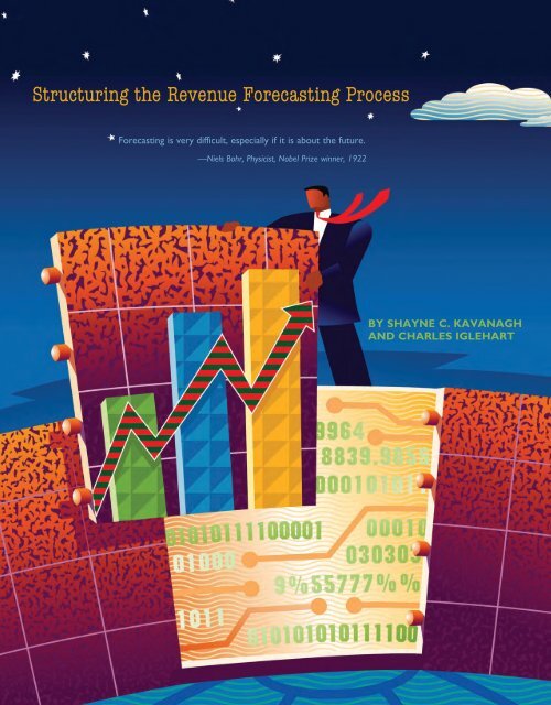
<strong>Structuring</strong> <strong>the</strong> <strong>Revenue</strong> <strong>Forecasting</strong> <strong>Process</strong><br />
<strong>Forecasting</strong> is very difficult, especially if it is about <strong>the</strong> future.<br />
—Niels Bohr, Physicist, Nobel Prize winner, 1922<br />
By Shayne C. Kavanagh<br />
and Charles Iglehart
Financial forecasting, which defines a government’s<br />
financial parameters, is one of <strong>the</strong> finance officer’s<br />
most important tasks. Accurate forecasting also forewarns<br />
a government about financial imbalances, allowing it to<br />
take action before a potential imbalance becomes a crisis, and<br />
forecasts can promote discussion about <strong>the</strong> future and how <strong>the</strong><br />
organization might develop long-term plans and strategies.<br />
This article describes a step-by-step approach to conducting<br />
revenue forecasts in local governments. As Bohr said,<br />
forecasting is not easy — but a structured approach can help<br />
forecasters ask <strong>the</strong> right questions, given <strong>the</strong> environment<br />
and audience; use <strong>the</strong> most appropriate techniques; and<br />
apply <strong>the</strong> lessons from one round of forecasting to future<br />
rounds. <strong>Structuring</strong> <strong>the</strong> forecasting process provides <strong>the</strong> following<br />
potential advantages:<br />
n <strong>Forecasting</strong> is easier to replicate each year, leading to<br />
greater organizational learning.<br />
n The process is transparent and relatively easy to explain<br />
to o<strong>the</strong>rs, which should make it easier to get o<strong>the</strong>rs to<br />
accept <strong>the</strong> forecasts.<br />
n Because a structured process<br />
encourages <strong>the</strong> forecaster to<br />
adhere to forecasting best practices<br />
more diligently than an unstructured<br />
method would, <strong>the</strong> results<br />
should be more accurate.<br />
The GFOA has adapted <strong>the</strong> following<br />
forecasting approach from <strong>the</strong><br />
advice of leading forecast scientists 1<br />
and <strong>the</strong> experiences<br />
of public finance practitioners and academic researchers.<br />
It involves <strong>the</strong> following steps: 2<br />
1. Define <strong>the</strong> Problem. What issues affect <strong>the</strong> forecast and<br />
presentation?<br />
2. Ga<strong>the</strong>r Information. Obtain statistical data, along with<br />
accumulated judgment and expertise, to support forecasting.<br />
3. Conduct a Preliminary/Exploratory Analysis. Examine<br />
data to identify major drivers and important trends. This<br />
establishes basic familiarity with <strong>the</strong> revenue being forecast.<br />
4. Select Methods. Determine <strong>the</strong> most appropriate quantitative<br />
and qualitative methods.<br />
5. Implement Methods. Use <strong>the</strong> selected methods to make<br />
<strong>the</strong> long-range forecast.<br />
STEP 1: DEFINE THE PROBLEM<br />
The first step in <strong>the</strong> forecasting<br />
process is to define <strong>the</strong> fundamental<br />
issues affecting <strong>the</strong> forecast.<br />
The first step in <strong>the</strong> forecasting process is to define <strong>the</strong> fundamental<br />
issues affecting <strong>the</strong> forecast, providing insight into<br />
which forecasting methods are most appropriate and how <strong>the</strong><br />
forecast is analyzed, as well as providing a common understanding<br />
as to <strong>the</strong> goals of <strong>the</strong> forecasting process. It will also<br />
help <strong>the</strong> forecasters think about what <strong>the</strong>ir audience might be<br />
interested in. While each local government will have distinct<br />
issues to consider, <strong>the</strong>re are three key questions that all governments<br />
should consider as part of Step 1.<br />
What is <strong>the</strong> Time Horizon of <strong>the</strong> Forecast? The time<br />
horizon affects <strong>the</strong> techniques and approach <strong>the</strong> forecaster<br />
will use. For example, short- and medium-term forecasts<br />
demand higher levels of accuracy because <strong>the</strong>y will be used<br />
for detailed budgeting decisions. Longer-term forecasts are<br />
used for more general planning, not detailed appropriations.<br />
Also, some forecasting techniques lend <strong>the</strong>mselves better to<br />
shorter- than longer-term forecasting, and vice versa. Longerterm<br />
forecasts will benefit from presentation techniques that<br />
emphasize <strong>the</strong> degree of uncertainty<br />
inherent in <strong>the</strong> forecast and <strong>the</strong> choices<br />
decision makers face.<br />
Is Our <strong>Forecasting</strong> Policy<br />
Conservative or Objective? An organization<br />
can adopt one of two basic<br />
policies on how forecasting will be<br />
conducted. A “conservative” approach<br />
systematically underestimates revenues<br />
to reduce <strong>the</strong> danger of budgeting more spending<br />
than actual revenues will be able to support. An “objective”<br />
approach estimates revenues as accurately as possible.<br />
Some public officials prefer conservative forecasts, which<br />
reduce <strong>the</strong> risk of a revenue shortfall. But this kind of forecast<br />
can also cause unnecessary fiscal stress during <strong>the</strong> budget<br />
process as <strong>the</strong> organization closes a fictitious revenue gap. At<br />
best, <strong>the</strong> government will incur opportunity costs, losing out<br />
on <strong>the</strong> benefits that could have been realized from programs<br />
and projects not undertaken. At worst, this approach could<br />
lead to unnecessary lay-offs or o<strong>the</strong>r disruptive cuts. Fur<strong>the</strong>r,<br />
overly conservative estimates could lead to lost credibility<br />
as budgeting personnel become increasingly weary of <strong>the</strong><br />
pseudo-financial stress.<br />
The downside of an objective approach is a greater chance<br />
of experiencing an actual revenue shortfall during <strong>the</strong> year<br />
October 2012 | <strong>Government</strong> <strong>Finance</strong> Review 9
and, thus, incurring actual fiscal stress during <strong>the</strong> course of<br />
<strong>the</strong> year, as <strong>the</strong> budget has to be adjusted. Organizations<br />
that pursue an objective policy of revenue estimating should<br />
develop policies and practices to guard against <strong>the</strong>se risks,<br />
such as budgetary reserve policies and contingency plans.<br />
Are We in a High or Low Growth Environment? Land<br />
uses underpin <strong>the</strong> fiscal health of local governments. Forecasters<br />
should consider if <strong>the</strong>ir community is experiencing: 3<br />
n High growth and development — <strong>the</strong> rate of population<br />
growth is increasing each year.<br />
n Moderate growth — <strong>the</strong>re is growth, but <strong>the</strong> rate is declining.<br />
n Low growth — population is declining or flat, or <strong>the</strong> rate<br />
of growth is negligible.<br />
Each of <strong>the</strong>se categories has different implications for <strong>the</strong><br />
forecast. For example, high-growth communities need to<br />
carefully consider <strong>the</strong> costs and benefits of potential new<br />
development, while low-growth communities are usually<br />
more concerned with modeling <strong>the</strong> financial impact of maintaining<br />
an aging infrastructure.<br />
STEP 2: GATHER INFORMATION<br />
The next step is to ga<strong>the</strong>r information supporting <strong>the</strong> forecasting<br />
process, including statistical data and <strong>the</strong> accumulated<br />
expertise of individuals inside and, perhaps, outside<br />
<strong>the</strong> organization.<br />
Take Stock of Economic Measures. Economic measures<br />
help provide context and might be directly useful in developing<br />
revenue assumptions. But first, you’ll need to understand<br />
<strong>the</strong> role of economic measures in forecasting for your community.<br />
The foremost question is whe<strong>the</strong>r relevant indicators<br />
are available. For example, small communities might not<br />
match up perfectly with an indicator<br />
for a large geographic area — unemployment,<br />
for instance. In this case,<br />
<strong>the</strong> indicator could provide context,<br />
but it probably wouldn’t be used in<br />
forecasting equations.<br />
People who are not part of <strong>the</strong><br />
organization can provide technical<br />
skills or resources that aren’t available<br />
in-house or aren’t economical to<br />
maintain, or <strong>the</strong>y can simply provide<br />
an outside perspective.<br />
For o<strong>the</strong>r governments, <strong>the</strong> geographic<br />
area covered by <strong>the</strong> indicator<br />
will match <strong>the</strong> jurisdiction well<br />
enough for direct use in forecasting.<br />
In this case, consider <strong>the</strong> quality of <strong>the</strong><br />
forecast for <strong>the</strong> indicator. Are credible,<br />
reliable future values available? For example, Fairfax<br />
County, Virginia, gets estimates of future employment in <strong>the</strong><br />
area from a third-party economic analysis firm. State and<br />
federal government agencies and universities will also often<br />
provide estimates of future values for select indicators. The<br />
Association for Budgeting and Financial Management maintains<br />
a database of state and local economic and financial<br />
indicators that can be accessed by <strong>the</strong> general public.<br />
Ga<strong>the</strong>r Inside and Outside Special Expertise. The<br />
finance officer should access special expertise from both<br />
inside and outside of <strong>the</strong> organization to improve forecasting.<br />
People who are not part of <strong>the</strong> organization can provide<br />
technical skills or resources that aren’t available in-house or<br />
aren’t economical to maintain, or <strong>the</strong>y can simply provide<br />
an outside perspective. One of <strong>the</strong> most common sources of<br />
external expertise is, of course, consultants, which can help<br />
with technical skills such as forecasting techniques, computer<br />
programs, or even cleaning and preparing historical data.<br />
Many governments also find that consultants bring additional<br />
credibility to <strong>the</strong> forecast as impartial, outside experts, and<br />
<strong>the</strong>y can help by raising issues that might not be difficult to<br />
talk about, o<strong>the</strong>rwise.<br />
Practitioners and researchers advise caution, however,<br />
when using consultants. Outside consultants almost never<br />
understand <strong>the</strong> jurisdiction’s unique political and economic<br />
circumstances as well as staff does, and this kind of understanding<br />
generally leads to <strong>the</strong> best forecasts. In addition,<br />
some consultants specialize in a particular forecasting technique<br />
and tend to apply it to all forecasting problems, but <strong>the</strong><br />
best technique depends on <strong>the</strong> particulars of <strong>the</strong> situation.<br />
Finally, if a consultant’s technique is too complex for staff<br />
to use on <strong>the</strong>ir own, staff might not be able to update <strong>the</strong><br />
forecast on time or adequately explain how <strong>the</strong> forecast was<br />
produced, diminishing credibility.<br />
Staff outside <strong>the</strong> finance department<br />
has information and perspectives that<br />
can supplement <strong>the</strong> forecast, so start<br />
accessing this accumulated expertise<br />
by holding regular internal meetings<br />
to review relevant indicators of economic<br />
and revenue. Participants can<br />
discuss whe<strong>the</strong>r <strong>the</strong> indicators are<br />
important or not, along with <strong>the</strong> trends<br />
shown by <strong>the</strong> indicators and <strong>the</strong>ir<br />
potential impact on forecasts.<br />
10 <strong>Government</strong> <strong>Finance</strong> Review | October 2012
Keep in mind that group interaction also has certain disadvantages,<br />
including <strong>the</strong> potential for participants to reinforce<br />
shared biases or for a dominant participant to take over <strong>the</strong><br />
proceedings, excluding o<strong>the</strong>r points of view. To mitigate<br />
<strong>the</strong>se problems, you can survey <strong>the</strong> people who have relevant<br />
expertise to supplement group interactions. The City<br />
of Dayton, Ohio, uses a survey to help forecast income tax<br />
revenue. Participants receive eight years of historical data,<br />
including <strong>the</strong> percentage change from year to year, and <strong>the</strong>n<br />
are asked to estimate final revenues for <strong>the</strong> current year and<br />
<strong>the</strong> next year. Dayton uses <strong>the</strong>se estimates to supplement<br />
o<strong>the</strong>r forecasting methods.<br />
Ga<strong>the</strong>r Historical <strong>Revenue</strong> Data. Good historical data<br />
are essential to good forecasting because past revenue patterns<br />
provide clues to future behavior. The first step is to<br />
compile revenue data for as many years back as is practical.<br />
This will often require scrubbing <strong>the</strong> data to remove <strong>the</strong><br />
impact of historical events that reduce <strong>the</strong>ir predictive value.<br />
For example, Fairfax County factored out a state-provided<br />
amnesty period for sales tax evaders that had brought in<br />
an additional $1.7 million in revenue. Only <strong>the</strong> data for <strong>the</strong><br />
most important revenues need be scrubbed in this manner,<br />
and <strong>the</strong> scrubbed data can be kept in a separate system (a<br />
spreadsheet is fine), as modifying data directly in <strong>the</strong> general<br />
ledger would obviously cause problems.<br />
Monthly data are best for mid-term (one to two years) and<br />
long-range (three to five years) forecasting. They are essentially<br />
for short-term forecasting because monthly data show<br />
trends more precisely, whereas more aggregated data such<br />
How Much Is Enough?<br />
Generally, forecasters should make every effort to ga<strong>the</strong>r<br />
at least five years of monthly data for forecasting. This is <strong>the</strong><br />
amount required to get a valid result from most statistical<br />
forecasting techniques and to give <strong>the</strong> forecaster a good<br />
sense of <strong>the</strong> historical trends behind <strong>the</strong> revenues.<br />
as annual figures can obscure important trends that occur<br />
within <strong>the</strong> year. Also, monthly data show seasonal variation,<br />
which is essential for short-term forecasting. If monthly data<br />
are not available, quarterly data can be used.<br />
STEP 3: CONDUCT A PRELIMINARY/<br />
EXPLORATORY ANALYSIS<br />
The objective of this step is to build <strong>the</strong> forecasters’ familiarity<br />
with and feel for <strong>the</strong> data. Forecasters do better if <strong>the</strong>y<br />
have insight into when and what quantitative techniques<br />
might be appropriate, and a better feel for <strong>the</strong> data can be<br />
helpful in more qualitative forms of forecasting. Forecasters<br />
look for consistent patterns or trends, such as <strong>the</strong> ones<br />
described below.<br />
Seasonality. Patterns that have reliably repeated <strong>the</strong>mselves<br />
are likely to continue into <strong>the</strong> future. It might also<br />
be necessary to use statistical techniques to “smooth out”<br />
seasonality and reveal a long-term trend line. Exhibit 1 shows<br />
an example of a seasonal pattern in sales taxes; Colorado<br />
Springs, Colorado, sees a jump from holiday spending and<br />
increases due to quarterly filings from smaller firms at three<br />
o<strong>the</strong>r points in <strong>the</strong> year.<br />
Business Cycles. Does <strong>the</strong> revenue (or expenditure) tend<br />
to vary with <strong>the</strong> level of economic activity in <strong>the</strong> community,<br />
or is it independent of cycles? Sales taxes on luxury goods<br />
often vary directly with business cycles, while sales taxes on<br />
consumer essentials remain fairly even.<br />
Outliers. Extreme values represent highly anomalous events<br />
that don’t add to <strong>the</strong> predictive power of <strong>the</strong> data set, and <strong>the</strong>y<br />
should be scrubbed out. Or <strong>the</strong>y could represent what author<br />
Nassim Nicholas Taleb has dubbed “black swan” events —<br />
highly unpredictable occurrences that can’t be forecasted<br />
but do hold lessons for <strong>the</strong> future. For instance, <strong>the</strong> “dot-com”<br />
stock market crash of 2001 may have foreshadowed <strong>the</strong> implications<br />
of <strong>the</strong> housing bust for some localities.<br />
October 2012 | <strong>Government</strong> <strong>Finance</strong> Review 11
Exhibit 1: Sales Tax Data from <strong>the</strong> City of Colorado Springs<br />
14<br />
12<br />
10<br />
Millions<br />
8<br />
6<br />
4<br />
2<br />
0<br />
January 2006<br />
June 2006<br />
November 2006<br />
April 2007<br />
September 2007<br />
February 2008<br />
July 2008<br />
December 2008<br />
May 2009<br />
October 2009<br />
March 2010<br />
August 2010<br />
January 2011<br />
June 2011<br />
November 2011<br />
April 2012<br />
Relationships between Variables. Correlation analysis is<br />
useful for determining important relationships between variables<br />
that could aid in forecasting. Forecasters use correlation<br />
analysis to compare revenues with predictive variables such<br />
as economic or demographic statistics, looking for strong relationships<br />
that can be used in quantitative forecasting or just to<br />
provide additional insight for judgmental forecasts. The most<br />
useful statistic is <strong>the</strong> correlation coefficient, often known simply<br />
as “r.” It measures <strong>the</strong> extent to which two variables move<br />
in <strong>the</strong> same or opposite directions and expresses this movement<br />
as a positive or a negative number. An r value of 1.0 is<br />
a perfect positive relationship, and -1.0 represents a perfect<br />
inverse relationship. A value of a zero indicates no relationship.<br />
Generally, an r value of more than 0.8 or less than -0.8<br />
would indicate a relationship worth exploring fur<strong>the</strong>r.<br />
A limitation of <strong>the</strong> standard correlation coefficient, however,<br />
is that it might not account for a lagging relationship<br />
between two variables. For example, enrollment would be<br />
a significant driver of tuition fees at a community college.<br />
And unemployment is often thought to motivate people to go<br />
back to school, so it would presumably have an impact on<br />
enrollment, as well. However, people do not typically enroll<br />
in a college course immediately after losing a job or failing to<br />
find employment. Hence, a correlation analysis of enrollment<br />
and regional unemployment figures would probably show a<br />
weak correlation for <strong>the</strong> same time period, but comparing<br />
enrollment to unemployment figures from earlier periods<br />
might show a stronger correlation.<br />
STEP 4: SELECT METHODS<br />
The next step is to determine <strong>the</strong> quantitative and/or qualitative<br />
forecasting methods to be used. <strong>Forecasting</strong> research<br />
has shown that “statistically sophisticated or complex methods<br />
do not necessarily produce more accurate forecasts than<br />
simpler ones.” 4<br />
While complex techniques might get more<br />
accurate answers in particular cases, simpler techniques tend<br />
to perform just as well or better, on average. Also, simpler<br />
techniques require less data, less expertise on <strong>the</strong> part of<br />
<strong>the</strong> forecaster, and less overall effort to use. Fur<strong>the</strong>r, simpler<br />
methods are easier to explain to <strong>the</strong> audience for <strong>the</strong> forecast.<br />
It makes sense to heed Einstein’s advice and make things “as<br />
simple as possible, but not simpler.”<br />
In <strong>the</strong> spirit of Einstein’s guidance, <strong>the</strong> GFOA has adapted<br />
Exhibit 2 from <strong>the</strong> work of J. Scott Armstrong. 5<br />
Armstrong<br />
originally published a flow chart to guide forecasters through<br />
Why Simple is Better — The Devil is in <strong>the</strong> Details<br />
Why do simple methods tend to outperform more complex<br />
ones? <strong>Forecasting</strong> science luminary Spyros Makridakis believes<br />
it is because complex methods try to find patterns that aren’t<br />
really <strong>the</strong>re by creating a tight statistical “fit” to historical data. *<br />
These false patterns are <strong>the</strong>n projected forward. Conversely,<br />
simple methods ignore such patterns and just extrapolate<br />
trends.<br />
* From: Spyros Makridakis, Robin M. Hogarth and Anil Gaba, “Why Forecasts Fail.<br />
What to Do Instead,” MIT Sloan Management Review, Winter 2010.<br />
12 <strong>Government</strong> <strong>Finance</strong> Review | October 2012
selecting a technique, across a comprehensive set of possible<br />
forecasting circumstances. The GFOA has modified <strong>the</strong><br />
chart to focus on <strong>the</strong> circumstances that are most relevant to<br />
public-sector financial forecasting and <strong>the</strong> techniques that<br />
appear most practical, given <strong>the</strong> limited resources available<br />
for forecasting that government organizations typically face.<br />
The flow chart begins with <strong>the</strong> availability of historical<br />
data. If data are not available or are in poor condition, expert<br />
judgment will likely be <strong>the</strong> best alternative — generating a<br />
number based on your feel for <strong>the</strong> situation. Research suggests<br />
that this is not an ideal approach, however, and that<br />
forecasters should always at least develop an algorithm to<br />
help guide <strong>the</strong> forecast. To illustrate, user fee revenue projections<br />
would be helped immensely by developing a simple<br />
model that multiplies <strong>the</strong> estimated price per unit sold by <strong>the</strong><br />
number of customers. A similar approach can be taken for<br />
o<strong>the</strong>r revenues.<br />
In many cases, and especially for important revenue<br />
sources, historical data will be available, and cleaning it up<br />
will not be cost prohibitive. Under <strong>the</strong>se circumstances, <strong>the</strong><br />
next question is about <strong>the</strong> forecaster’s knowledge of <strong>the</strong> relationships<br />
between <strong>the</strong> item being forecast and independent<br />
variables that help explain that item’s behavior. For example,<br />
is <strong>the</strong>re a significant relationship between certain economic<br />
indicators and revenue yield? Finding significant relationships<br />
can be difficult, especially in small governments, because<br />
<strong>the</strong>re aren’t enough locally relevant economic indicators<br />
or because contextual events have a big impact on revenue<br />
yield. This leads to <strong>the</strong> question of whe<strong>the</strong>r <strong>the</strong> forecaster has<br />
good domain knowledge, or knowledge of <strong>the</strong> local financial<br />
and economic environment, which allows individual expertise<br />
to be combined with an extrapolation of historical trends.<br />
If you don’t have good domain knowledge, you will likely be<br />
better off using extrapolation techniques without judgmental<br />
adjustment.<br />
Exhibit 2: Selecting <strong>Forecasting</strong> Methods<br />
No<br />
Sufficient Historical<br />
Data Available?<br />
Yes<br />
Expect Judgment<br />
<strong>Forecasting</strong><br />
No<br />
Good Knowledge<br />
of Relationships?<br />
Yes<br />
Good Domain<br />
Knowledge?<br />
Yes<br />
No<br />
No<br />
Large Changes<br />
Expected?<br />
Yes<br />
Extrapolation-<br />
Judgment Hybrid<br />
Extrapolation<br />
Econometric<br />
Methods<br />
Different<br />
Methods<br />
Provide Useful<br />
Forecasts?<br />
Use Selected<br />
Method<br />
No<br />
Yes<br />
Combine<br />
Forecasts<br />
October 2012 | <strong>Government</strong> <strong>Finance</strong> Review 13
Exhibit 3: Results of <strong>Forecasting</strong> Technique Accuracy Experiment<br />
Mean Absolute Percent Average Percent Error Number of Times Number of Times<br />
Error for Months for Entire Year It Was Best (of 8) It Was Worst (of 8)<br />
Single Exponential Smoothing 12.38 4.46 3 0<br />
12-Month Moving Average 12.68 5.40 1 1<br />
Simple Trending 18.47 13.19 1 5<br />
Time Series Regression 15.39 9.29 3 2<br />
If you do have good knowledge of <strong>the</strong> relationships<br />
between <strong>the</strong> dependent and independent variables, <strong>the</strong> next<br />
question is whe<strong>the</strong>r large changes are expected. In <strong>the</strong> context<br />
of government revenue forecasting, large changes are<br />
most likely to occur over a long time period, so econometric<br />
methods might be more useful for long-term forecasting. If<br />
you do not expect large changes, you are probably better<br />
off using extrapolation techniques, perhaps combined with<br />
expert judgment, if your domain knowledge is good. The<br />
choice between forecasting methods is not always clear cut,<br />
and if more than one method appears useful, <strong>the</strong> results can<br />
be combined.<br />
Of course, accuracy is also important when selecting<br />
a forecasting method. The GFOA conducted a very basic<br />
forecasting experiment with historical sales tax data from<br />
seven local governments and income taxes from one, using<br />
relatively simple techniques to project revenues 12 months<br />
into <strong>the</strong> future. Econometric forecasting was excluded from<br />
<strong>the</strong> analysis since that technique is generally better suited to<br />
longer-term forecasts. The analysis focused on sales tax data,<br />
since sales taxes have <strong>the</strong> reputation of being volatile and,<br />
<strong>the</strong>refore, harder to predict.<br />
Exhibit 3 summarizes <strong>the</strong> results. Single exponential<br />
smoothing, which is a relatively simple extrapolation technique,<br />
clearly appears to have <strong>the</strong> greatest accuracy. It has<br />
<strong>the</strong> lowest percentage of error, and it was tied for <strong>the</strong> number<br />
of times it was <strong>the</strong> best-performing technique, as well as being<br />
a close second in three o<strong>the</strong>r cases.<br />
And it was never <strong>the</strong> worst-performing<br />
technique, which means that it will<br />
often be very accurate and seldom<br />
be highly inaccurate. For <strong>the</strong> entire<br />
year, exponential smoothing predicted<br />
total revenues within 3 percent five<br />
future behavior.<br />
times, and two of those times were<br />
within 1 percent.<br />
Good historical data are essential<br />
to good forecasting because past<br />
revenue patterns provide clues to<br />
The o<strong>the</strong>r techniques tested had varying degrees of success.<br />
The premise behind moving average forecasting is similar to<br />
that of single exponential smoothing, so it isn’t surprising that<br />
moving average forecasting appears to be <strong>the</strong> second-best<br />
technique, overall. The results of time series regression were<br />
mixed; on one hand, it was <strong>the</strong> best-performing technique<br />
three times (tied with exponential smoothing), and it predicted<br />
annual revenues within 3 percent on three occasions, two<br />
of those within 1 percent. On <strong>the</strong> o<strong>the</strong>r hand, it was also <strong>the</strong><br />
worst-performing technique twice, producing annual errors<br />
of 23 percent and 14 percent. In comparison, <strong>the</strong> worst error<br />
produced by exponential smoothing was 11 percent. Simple<br />
trending is clearly <strong>the</strong> worst technique, often producing<br />
substantial errors and rarely producing an accurate forecast<br />
(although it did produce <strong>the</strong> best results in one case).<br />
Given <strong>the</strong>se results, it would appear that revenue forecasters<br />
should always at least consider using single exponential<br />
smoothing, which puts a heavier weighting on recent periods;<br />
this probably explains its superior performance. Moving averages<br />
might present a reasonable secondary option, if single<br />
exponential smoothing is too complex to use, for example.<br />
Time series regression is also worth considering, but it<br />
assumes a linear relation between time and revenue yields, so<br />
you must be certain that this assumption holds. It’s also possible<br />
that larger governments will experience better results<br />
with time series regression, since <strong>the</strong> diversity of <strong>the</strong>ir revenue<br />
bases means that <strong>the</strong>re is less variability<br />
in <strong>the</strong>ir yields, <strong>the</strong>reby making<br />
it easier to “fit” a regression equation<br />
to <strong>the</strong> historical data. Indeed, <strong>the</strong> largest<br />
four governments in <strong>the</strong> GFOA’s<br />
data set had an average error for <strong>the</strong><br />
year of 3.7 percent, using regression,<br />
compared to 9.29 percent for all eight<br />
governments. Simple trending should<br />
14 <strong>Government</strong> <strong>Finance</strong> Review | October 2012
probably be avoided in most cases. Although it did work well<br />
in one case, it produced substantial errors in o<strong>the</strong>rs (more<br />
than 40 percent, in two cases).<br />
STEP 5: IMPLEMENT METHODS<br />
Once <strong>the</strong> methods have been selected, <strong>the</strong>y can be used<br />
to make a forecast. This section will explain <strong>the</strong> concept of<br />
averaging forecasting methods and developing a range of<br />
possible forecast results.<br />
Averaging Methods. Research shows that averaging <strong>the</strong><br />
results of multiple forecasting methods produces better<br />
results than using any one method alone. One oft-cited study<br />
tested averages of different combinations of 14 quantitative<br />
forecast techniques, comparing <strong>the</strong> results of each technique<br />
in isolation with <strong>the</strong> averages of up to 10 of <strong>the</strong> techniques. 6<br />
The results showed large and consistent reductions in error<br />
across a variety of situations, some of which are displayed in<br />
Exhibit 4. Many researchers cite between four and five models<br />
as <strong>the</strong> number necessary to gain <strong>the</strong> benefits from averaging<br />
(results did continue to improve beyond that, but <strong>the</strong>y<br />
were inconsequential). Averaging even two or three forecasts<br />
could reduce “noise” and better reveal <strong>the</strong> underlying pattern,<br />
as Exhibit 4 shows. In fact, <strong>the</strong>se researchers found that<br />
even <strong>the</strong> technique that performed best in isolation could<br />
be improved (albeit slightly) by averaging it with just two to<br />
three o<strong>the</strong>r high-performing techniques.<br />
Exhibit 4: Reduction in Error<br />
from Averaging Forecasts<br />
Number Percent Percent Percent<br />
of Forecasts of Monthly of Yearly of All<br />
Averaged Data Data Data<br />
5 16.4 9.1 16.3<br />
4 14.3 8.5 14.3<br />
3 11.4 7.6 11.5<br />
2 6.9 5.7 7.2<br />
Exhibit 5: Calculating a Prediction Interval<br />
PI = (<strong>the</strong> forecast number) +/- (1.65 x square root of mean<br />
squared error of historical data)<br />
Averaging can also work with purely judgmental forecasts.<br />
The error associated with <strong>the</strong>se forecasts, much less averages<br />
of <strong>the</strong>m, have not been studied in nearly as much depth as<br />
quantitative forecasts, so <strong>the</strong> guidance on how many forecasts<br />
to average is not as definitive. Leading forecast scientist<br />
Spyros Makridakis suggests five to seven contributors as a<br />
minimum to aim for, although fewer contributors are necessary<br />
if you are using a hybrid of quantitative and judgmental<br />
techniques. 7<br />
Forecast Ranges. Forecasts are often expressed as “point<br />
forecasts” because <strong>the</strong>y express future revenues as a single<br />
number, although this number is actually made up of averages<br />
— averages of historical experiences and perhaps averages<br />
of different forecasting techniques. Presenting one number<br />
obscures variability, since <strong>the</strong> possible future outcomes are<br />
many. Hence, it might be wise to develop a range of possible<br />
forecast outcomes — known in forecasting science as “prediction<br />
intervals.” Prediction intervals illustrate uncertainty in<br />
<strong>the</strong> forecast by showing a range around <strong>the</strong> baseline forecast<br />
in which <strong>the</strong> forecaster believes <strong>the</strong> actual value will fall,<br />
expressed in probabilities (e.g., <strong>the</strong> actual value is 90 percent<br />
certain to fall between X and Y). Research shows that some<br />
forecast users prefer prediction intervals over point forecasts<br />
because prediction intervals better demonstrate future<br />
uncertainties and assist in planning for alternative strategies<br />
that address <strong>the</strong> range of future outcomes. 8<br />
However, many<br />
members of <strong>the</strong> forecaster’s audience are probably not accustomed<br />
to thinking in terms of probabilities, so prediction<br />
intervals might take some getting used to.<br />
The formula in Exhibit 5 shows how to calculate a prediction<br />
interval for a one-step-ahead forecast (e.g., a forecast for<br />
<strong>the</strong> period immediately following <strong>the</strong> last available actual<br />
statistics). The prediction internal (PI) is equal to <strong>the</strong> forecast<br />
plus-and-minus a constant, which is multiplied by <strong>the</strong> square<br />
root of <strong>the</strong> mean squared error. Our example uses a constant<br />
of 1.65, which produces a 90 percent interval. This constant is<br />
known as a “z score,” and <strong>the</strong> z scores necessary to produce<br />
o<strong>the</strong>r intervals can be easily obtained from <strong>the</strong> Internet and<br />
most statistical texts. The mean squared error is simply <strong>the</strong><br />
average of <strong>the</strong> squared difference between <strong>the</strong> actual and<br />
forecasted value for every point in <strong>the</strong> data set. Squaring <strong>the</strong><br />
error removes any negative sign. A square root is <strong>the</strong>n taken<br />
to reduce <strong>the</strong> number back to a magnitude relevant to <strong>the</strong><br />
data set.<br />
While <strong>the</strong> formula for one-step-ahead prediction intervals is<br />
simple enough, a statistical calculation becomes increasingly<br />
October 2012 | <strong>Government</strong> <strong>Finance</strong> Review 15
complex for multiple steps ahead. This<br />
is because <strong>the</strong> mean square error statistic<br />
from Exhibit 5 is based on onestep-ahead<br />
forecasts, so it must be<br />
modified to reflect <strong>the</strong> average error<br />
in making <strong>the</strong> “n”-step-ahead forecast<br />
that that <strong>the</strong> forecaster is interested<br />
in — and this must be repeated for<br />
every n value of interest. The statistical<br />
method can become tedious and<br />
complex, so researchers have offered<br />
alternatives.<br />
You can set <strong>the</strong> prediction interval<br />
using your own judgment, but research has shown that confidence<br />
intervals set this way are usually too narrow (i.e., <strong>the</strong><br />
forecaster is overconfident or underestimates <strong>the</strong> amount of<br />
variability), likely because <strong>the</strong> point forecast becomes an<br />
anchor from which <strong>the</strong> forecaster unconsciously hesitates to<br />
stray. 9 Following are two ways to deal with this problem.<br />
One way is to calculate a one-step-ahead prediction interval<br />
using <strong>the</strong> formula in Exhibit 5, since it is relatively simple<br />
to do. This might serve as a starting point, or an anchor, for<br />
judgmentally developing prediction internals for n-step-ahead<br />
forecasts. The interval should widen as n becomes larger,<br />
since <strong>the</strong>re will presumably be greater uncertainty <strong>the</strong> far<strong>the</strong>r<br />
<strong>the</strong> forecast goes into <strong>the</strong> future.<br />
Ano<strong>the</strong>r approach is to simply widen a judgmentally<br />
set prediction interval. First decide <strong>the</strong> interval probability<br />
(e.g., 90 percent, 80 percent, etc.) and <strong>the</strong>n ask a series of<br />
knowledgeable judges to estimate <strong>the</strong> range of upper and<br />
lower values that would include 90 percent (or 80 percent or<br />
whatever probability you selected) of all possible outcomes.<br />
Average all <strong>the</strong> results toge<strong>the</strong>r to get an interval. This interval<br />
will likely be too narrow, so double it. 10<br />
The second alternative to <strong>the</strong> prediction interval statistical<br />
formula uses historical data but doesn’t rely on statistical<br />
techniques. Take <strong>the</strong> difference between <strong>the</strong> largest and<br />
smallest observation in <strong>the</strong> historical data set and multiply<br />
by 1.5, although if you have very small set of data, you might<br />
need to use a multiplier as high as 2. This range is thought<br />
to be a crude estimation of a 95 percent prediction interval. 11<br />
You can divide <strong>the</strong> range by two and add <strong>the</strong> result to or<br />
subtract it from <strong>the</strong> forecast to get <strong>the</strong> forecast range. Again,<br />
remember that <strong>the</strong> fur<strong>the</strong>r forecasts go into <strong>the</strong> future, <strong>the</strong> less<br />
Forecasters do better if <strong>the</strong>y<br />
have insight into when and what<br />
quantitative techniques might be<br />
appropriate, and a better feel for<br />
<strong>the</strong> data can be helpful in more<br />
qualitative forms of forecasting.<br />
reliable <strong>the</strong>y become, so <strong>the</strong> prediction<br />
interval should widen as it moves<br />
away from <strong>the</strong> origin.<br />
CONCLUSIONS<br />
<strong>Revenue</strong> forecasting helps local governments<br />
better plan future service levels<br />
and anticipate financial challenges.<br />
This article has presented a structured<br />
approach to <strong>the</strong> revenue forecasting<br />
process in order to help finance officers<br />
produce a more replicable, transparent,<br />
and accurate forecast. y<br />
Notes<br />
1. Particularly Principles of <strong>Forecasting</strong> by J. Scott Armstrong and<br />
<strong>Forecasting</strong>: Methods and Applications by Spyros Makridakis, et al..<br />
2. Forecasters should also consider how <strong>the</strong> forecasts will be used and<br />
how <strong>the</strong> process should be evaluated, but those are beyond <strong>the</strong> scope<br />
of this article.<br />
3. Rebecca M. Hendrick, author of Managing <strong>the</strong> Fiscal Metropolis, contributed<br />
to this section.<br />
4. Quote from Spyros Makridakis and Michele Hibon, “The M-3<br />
Competition: Results, Conclusions, and Implications,” International<br />
Journal of <strong>Forecasting</strong> 16 (2000). The “M Competitions” were a series<br />
of three forecasting accuracy tests conducted over almost 20 years by<br />
Makridakis and colleagues. The results have been widely studied, replicated,<br />
and cited.<br />
5. See J. “Scott Armstrong, “Selecting <strong>Forecasting</strong> Methods,” 2009.<br />
Available at www.forecastingprinciples.com. The paper is an updated<br />
version of Armstrong’s chapter on <strong>the</strong> same subject in Principles of<br />
<strong>Forecasting</strong>.<br />
6. Spyros Makridakis and Robert L. Winkler, “Averages of Forecasts: Some<br />
Empirical Results.” Management Science, Vol. 29, No. 9. September 1983.<br />
7. Spyros Makridakis, Robin Hogarth, and Anil Gaba, Dance with Chance:<br />
Making Luck Work for You (Oneworld Publications: Oxford, England) 2009.<br />
8. Michael Lawrence, Paul Goodwin, Marcus O’Connor, and Dilek Onkal,<br />
“Judgmental <strong>Forecasting</strong>: A Review of Progress Over <strong>the</strong> Last 25 Years,”<br />
International Journal of <strong>Forecasting</strong>, Vol 22. 2006.<br />
9. “Overconfidence” does not necessarily mean that <strong>the</strong> forecaster has an<br />
inflated sense of his or her abilities, but that <strong>the</strong> forecaster underestimates<br />
variability.<br />
10. Makridakis, et al., Dance With Chance.<br />
11. Spyros Makridakis, Robin M. Hogarth and Anil Gaba, “Why Forecasts<br />
Fail. What to Do Instead,” MIT Sloan Management Review, Winter 2010.<br />
SHAYNE C. KAVANAGH is senior manager of research for <strong>the</strong><br />
GFOA’s Research and Consulting Center in Chicago, Illinois. He<br />
can be reached at skavanagh@gfoa.org. CHARLES IGLEHART is a<br />
volunteer researcher for <strong>the</strong> GFOA. He recently obtained his M.S. in<br />
applied ma<strong>the</strong>matics from DePaul University and is pursuing actuarial<br />
certification.<br />
16 <strong>Government</strong> <strong>Finance</strong> Review | October 2012