Experiment 3 - Transmission Lines, Part 1

Experiment 3 - Transmission Lines, Part 1
Dr. Haim Matzner & Shimshon Levy.
August, 2008.

Contents
Introduction 1
0.1 Prelab Exercise . . . . . . . . . . . . . . . . . . . . . . . . . . 1
0.2 Background Theory . . . . . . . . . . . . . . . . . . . . . . . . 1
0.2.1 Characteristic Impedance . . . . . . . . . . . . . . . . 5
0.2.2 Terminated Lossless Line . . . . . . . . . . . . . . . . . 6
0.2.3 The Impedance Transformation . . . . . . . . . . . . . 8
0.3 Shorted Transmission Line . . . . . . . . . . . . . . . . . . . . 9
0.3.1 Open Circuit Line- . . . . . . . . . . . . . . . . . . . . 12
0.3.2 Low Loss Line . . . . . . . . . . . . . . . . . . . . . . . 12
0.4 Calculating Transmission Line parameters by Measuring Z 0 , α, and
β . . . . . . . . . . . . . . . . . . . . . . . . . . . . . . . . . . 13
0.4.1 Calculating Coaxial Line Parameters by Measuring
Physical Dimensions . . . . . . . . . . . . . . . . . . . 14
Experiment Procedure 17
0.5 Required Equipment . . . . . . . . . . . . . . . . . . . . . . . 17
0.6 Phase Difference of Coaxial Cables, Simulation and Measurement
. . . . . . . . . . . . . . . . . . . . . . . . . . . . . . . . 17
0.7 Wavelength of Electromagnetic Wave in Dielectric Material . . 18
0.8 Input Impedance of Short - Circuit Transmission Line . . . . . 20
0.9 Impedance Along a Short - Circuit Microstrip Transmission
Line . . . . . . . . . . . . . . . . . . . . . . . . . . . . . . . . 22
0.10 Final Report . . . . . . . . . . . . . . . . . . . . . . . . . . . . 24
0.11 Appendix-1 - Engineering Information for RF Coaxial Cable
RG-58 . . . . . . . . . . . . . . . . . . . . . . . . . . . . . . . 25
v

Introduction
0.1 Prelab Exercise
• 1. Define the terms: Relative permittivity, dielectric loss tangent
(tan δ), skin depth and distributed elements.
2. Refer to Figure 1, find the frequency that will cause a 2π radians phase
difference between the two RG-58 coaxial cables, assume µ R = 1, ɛ r = 2.3.
a. Find the relative amplitude of the two signals.
b. Verify your answers in the laboratory.
Signal generator
515.000,00 MHz
0.7m RG-58
Oscilloscope
3.4m RG-58
Figure 1 -Phase difference between two coaxial cables.
0.2 Background Theory
Transmission lines provide one media of transmitting electrical energy between
the power source to the load. Figure 2 shows three different geometry
types of lines used at microwave frequencies.
1

2 CHAPTER 0 INTRODUCTION
Coaxial cable
Two paralel
wire line
Microstrip
Line
Figure 2 - Popular transmission lines.
Rectangular metal
waveguide
The open two-wire line is the most popular at lower frequencies, especially
for TV application. Modern RF and microwave devices practice involves
considerable usage of coaxial cables at frequencies from about 10 MHz up to
30 GHz and hollow waveguides from 1 to 300 GHz.
A uniform transmission line can be defined as a line with distributed
elements, as shown in Figure 3.
R’ = Series resistance per unit length of line (Ω/m).
Resistance is related to the dimensions and conductivity of the metallic
conductors, resistance is depended on frequency due to skin effect.
G’ = Shunt conductance per unit length of line (/m).
G’ is related to the loss tangent of the dielectric material between the two
conductors. It is important to remember that G’ is not a reciprocal of R’.
They are independent quantities, R’ being related to the various properties
of the two conductors while G’ is related to the properties of the insulating
material between them.

0.2 BACKGROUND THEORY 3
First section Second section Third-section
R/2 L/2 L/2 R/2
ZG
G C G C G
C
Equivalent circuit of transmission line
z=0
Figure 3 -Transmission lines model
L ’ = Series inductance per unit length of line (H/m).
L’- Is associated with the magnetic flux between the conductors.
C’ = Shunt capacitance per unit length of line (F/m).
C’- Is associated with the charge on the conductors.
Naturally, a relatively long piece of line would contain identical sections as
shown. Since these sections can always be chosen to be small as compared to
the operating wavelength. Hence the idea is valid at all frequencies. The series
impedance and the shunt admittance per unit length of the transmission
line are given by:
Z = R ′ + JωL ′
Y = G ′ + JωC ′
The expressions for voltage and current per unit length are given respectively
by equations (1) and (2):
dV (z)
dz
dI(z)
dz
= −I(z)(R ′ + JωL ′ ) (1)
= −V (z)(G ′ + JωC ′ ) (2)
Where the negative sign indicates on a decrease in voltage and current as z
increases. The current and voltage are measured from the receiving end; at
z = 0 and line extends in negative z-direction. The differentiating equations,
(3) and (4), associate the voltage and current:

4 CHAPTER 0 INTRODUCTION
d 2 V (z)
dz
d 2 I(z)
dz
Where
= −(R ′ + JωL ′ ) dI(z)
dz
= −(G ′ dV (z)
+ JωC)
dz
= (G ′ + JωC ′ )(R ′ + JωL ′ )V (z) = γ 2 V (z) (3)
= (G ′ + JωC ′ )(R ′ + JωL ′ )I(z) = γ 2 I(z)(4)
γ = √ ZY = √ (G ′ + jωC ′ )(R ′ + jωL ′ ) (5)
The above equations are known as wave equations for voltage and current,
respectively, propagating on a line. The solutions of voltage and current
waves are:
V (z) = V 1 e −γz + V 2 e +γz (6)
I(z) = I 1 e −γz + I 2 e +γz
These solutions are shown as the sum of two waves; the first term ,V 1 , indicates
the wave traveling in positive z-direction, and is called the incident
wave, while the second term, V 2 , indicates the wave traveling in the negative
z-direction, and is called the reflected wave. γ is a complex number that is
called the propagation constant and can be defined as:
γ = α + jβ (7)
α is called the attenuation constant of the propagating wave, α is the real part
of Eq. (2.7) while β is the imaginary part and is called the phase constant.
Thus, propagation constant γ is the phase shift and attenuation per unit
length along the line. Separating equation (2.5) into real and imaginary
parts, we can get:
α =
β =
[√
(G
′2
+ ω 2 C 2 )(R ′2 + ω 2 L ′2 ) + (R ′ G ′ − ω 2 L ′ C ′ )
[√
(G
′2
+ ω 2 C ′2 )(R ′2 + ω 2 L ′2 ) − (R ′ G ′ − ω 2 L ′ C ′ )
2
2
] 1
2
] 1
2
(8)
(9)
α is measured in nepers per unit length of the transmission line (1 neper
= 8.686dB). β is measured in radians per unit length of tthe transmission

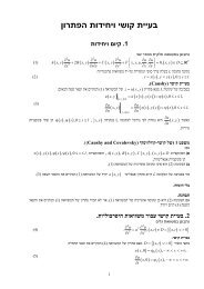
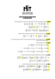
0.2 BACKGROUND THEORY 5
line. That means that β can be calculated as:
β = 2π λ
(10)
Where λ is the wavelength or distance along the line corresponding to a phase
change of 2π radians. If the wavelength in free space is denoted by λ 0 , then:
λ 0 = c = v √
p ɛR µ R
= λ √ ɛ R µ
f 0 f
R (11)
Where c is the velocity of light in free space and v p is the velocity of electric
wave in a dielectric material.
0.2.1 Characteristic Impedance
If RF voltage V is applied across the conductors of an infinite line, it causes a
current I to flow. By this observation, the line is equivalent to an impedance,
which is known as the characteristic impedance, Z 0 :
Z 0 = V (z)
I(z)
The expression for current I, using Eqs. (2.1) and (2.6), is given by:
Where
1
I = −
(R ′ + JωL ′ )
I 1 =
∂V
∂z = − 1
(R ′ + JωL ′ ) (−γ)(V 1e −γz + V 2 e +γz )
I(z) = I 1 e −γz + I 2 e +γz
V 1
(R ′ + JωL ′ ) (γ) and I 2 =
V 2
(R ′ + JωL ′ ) (γ)
Infinite line has no reflection, therefore I 2 = V 2 = 0 and:
V (z)
I(z) = V 1
I 1
=
(R ′ + JωL ′ )
√
(R′ + JωL ′ )(G ′ + JωC ′ )
Thus the characteristic impedance of infinite line can be calculated by (12):
√
Z 0 = V (z)
I(z) = (R ′ + JωL ′ )
(12)
(G ′ + JωC ′ )

6 CHAPTER 0 INTRODUCTION
Line Impedance
We can rewrite the current and voltange along the line as:
V (z) = V 1 e −γz + V 2 e +γz (13)
I(z) = V 1
Z 0
e −γz + V 2
Z 0
e +γz
and the line impedance (the impedance at point z) as:
Z(z) = V (z)
I(z) = Z 0 (V 1 e −γz + V 2 e +γz )
V 1 e −γz − V 2 e +γz (14)
0.2.2 Terminated Lossless Line
Consider a lossles line, length l, terminated with a load Z L , as shown in
Figure 4.
I(z)
I L
V(z)
V L
Z l
z = −l
l
z
=
0
Figure 4 - A transmission line, terminated with a load.
Using equation (2.13) and recalling that α = 0, one can define the current
and voltage on the load terminal (at z = 0) as:
V L
I L
= Z L (15)
V (z = 0) = V 1 e −jβ(0) + V 2 e jβ(0) = V 1 + V 2 (16)
I(z = 0) = V 1
Z 0
e −jβ(0) − V 2
Z 0
e jβ(0) = V 1
Z 0
+ V 2
Z 0

0.2 BACKGROUND THEORY 7
We can also add the boundary conditions:
V (z = 0) = V L (17)
I(z = 0) = I L
Using equation (2.16) we can rewrite (2.15) as equation (2.18):
Z L = V L
I L
=
V (z = 0)
I(z = 0) = V 1 + V 2
V 1
Rearranging equation (2.18) one can rewrite:
V 2
Z 0
+ V 2
Z 0
(18)
= Z L − Z 0
⊜ Γ
V 1 Z L + Z 0
Where Γ is the complex reflection coefficient. It relates to the magnitude and
phase of the reflected wave (V 2 ) emerging from the load and to the magtitude
and phase of the incident wave (V 1 ) , or
Equation (2.13) can be rewrite as:
V 2 = ΓV 1 (19)
V (z) = V 1 e −jβz + ΓV 1 e jβz (20)
I(z) = V 1
Z 0
e −jβz − Γ V 1
Z 0
e jβz
The reflection coefficient at an arbitrary point along the transmission line is:
Γ(z) = V 2e −jβz
= Γ(0)e−2jβz
V 1 e−jβz While the time average power flow along the line at point z is:
P av = 1 2 Re[V (z)I(z)∗ ] (21)
= 1 2
V 2
1
Z 0
Re ( 1 − Γ ∗ e −j2βz + Γe j2βz − |Γ| 2)
When recalling that Z − Z ∗ = 2j Im Z, equation (2.21) can be simplified to:
P av = 1 2
V 2
1
Z 0
(
1 − |Γ|
2 ) (22)
Which shows that the average power flow is constant at any point on the
lossless transmission line. If Γ = 0 (perfect match), the maximum power is
delievered to the load, while all the power is reflected for Γ = 1.

8 CHAPTER 0 INTRODUCTION
0.2.3 The Impedance Transformation
According to the transmission line theory, in a short circuit line, the impedance
become infinite at a distance of one-quarter wavelength from the
short. The ability to change the impedance by adding a length of transmission
line is a very important attribute to every RF or microwave designer.
If we look at the transmission line (losseless line), as illustrated in Figure 5,
and use equation (2.20), the line impedance at z = −l (input impedance)
is:
Z in =
V (z = −l)
I(z = −l) = Z 0
( )
e jβl + Γe −jβl
e jβl − Γe −jβl
(23)
l
I L
I (z)
ZG
Z in
Z 0
β
V L
ZL
z = −l
z = 0
Figure 5 -Transmission line terminated in arbitrary impedance Z L .
If we use the relationship Γ = (Z L − Z 0 ) / (Z L + Z 0 ) with equation (2.23) we
get:
( (
ZL e jβl + e −jβl) (
+ Z 0 e jβl − e −jβl)
)
Z in = Z 0 (24)
Z L (e jβl + Γe −jβl ) − Z 0 (e jβl − e −jβl )
By recalling Euler’s equations:
e jβl
e −jβl
= cos βl + j sin βl
= cos βl − j sin βl
We can get:
( )
ZL cos βl + jZ 0 sin βl
Z in = Z 0
Z 0 cos βl + jZ L sin βl
Or:
( )
ZL + jZ 0 tan βl
Z in = Z 0
Z 0 + jZ L tan βl
Lets examine special cases:
(25)

0.3 SHORTED TRANSMISSION LINE 9
0.3 Shorted Transmission Line
The voltage and current along a transmission line as a function of time is
known as:
[
V (z, t) = A cos ω
(t − z ) ] [
+ θ + B cos ω
(t + z ) ]
+ φ (26)
v p v p
I(z, t) = 1 [ {A cos ω
(t − z ) ] [
+ θ − B cos ω
(t + z ) ]}
+ φ
Z 0 v p v p
Where z = 0, at the generator side, and d = 0 at the load side, as shown in
Figure 6.
z=d
z
V
Z 0
I(z)
, β
z
z=0
Figure 6 -Shorted transmission line.
This expression can be rewrite in phasor form as:
V (z) = V 1 e −jβz + V 2 e jβz (27)
I(z) =
1 (
V1 e −jβz − V 2 e jβz)
Z 0
Where V 1 = Ae jθ is the forward wave, V 2 = Be jϕ is the reflected wave and
β = ω/v p .The boundary condition for the short circuit transmission line at
z = 0 is that the voltage across the short circuit is zero:
Using equations (27) and (28), we obtain:
V (0) = 0 (28)

10 CHAPTER 0 INTRODUCTION
V (0) = V 1 e jβ0 + V 2 e −jβ0 = 0 (29)
V 1 = −V 2
Inserting Eq (29) into Eq (28), we get:
V (z) = V 1 e jβz − V 1 e −jβz = 2jV 1 sin βz (30)
I(z) = 1 Z 0
(
V1 e jβz + V 1 e −jβz) = 2 V 1
Z 0
cos βz
Which shows that the V = 0 at the load end, while the current is a maximum
there. The ratio between V(z) and I(z) is the input impedance and is equal
to:
Z in = jZ 0 tan βz (31)
Which is purely imaginary for any length of z. The value of Z in(sc) vary
between +j∞ to −j∞, every π/2 (λ/4),by changing z, the length of the
line, or by changing the frequency. The voltage and current as a function of
time and distance are:
V (z, t) = Re [ V (z)e jωt] (32)
= Re ( 2e jπ/2 |V 1 | e jθ e jωt sin βz )
= −2 |V 1 | sin βz sin (ωt + θ)
Where V 1 = |V 1 | e jθ and j = e jπ/2 .
I(z, t) = Re [ I(z)e jωt] (33)
(
= Re 2 V )
1
cos βze jωt
Z 0
2
= |V 1 | cos βz cos (θ + ωt)
Z 0

0.3 SHORTED TRANSMISSION LINE 11
Figure 7 -Voltage along a shorted transmission line, as a function of time
and distance from the load. Frequency 1GHz.
The result of the voltage on the shorted transmission line is shown in
figure 7, assume that V 1 = sin 2π10 9 t (λ = 30cm) , which shows that :
• The line voltage is zero for βz = 0 + nπ n = 0, 1, 2...for all value of
time.
• The voltage at every point of z is sinusoidal as a function of time. The
maximum absolute value of the voltage is known as a standing wave
pattern.
Impedance
magnitude
Frequency difference
0 Wavelengths 1 (λ)
2
Figure 8 - Input impedance of shorted low loss coaxial cable.

12 CHAPTER 0 INTRODUCTION
0.3.1 Open Circuit Line-
For lossless line α ≠ 0 and Y L = 0, equation (2.25) is reduce to:
or in impedance form:
Y in = Y 0 tan βz
Z in(os) = Z 0
tan βz
(34)
Using Eqs. (2.24), (2.34) and (2.35), Z 0 can be computed from the short and
open circuit, by the relation:
Z 0 = √ Z in(sc) Z in(os)
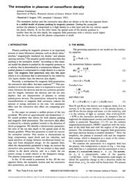
0.3.2 Low Loss Line
In many cases, the loss of microwave transmission lines is small. In these
cases, some approximation can be made that simplify the expression of propagation
constant γ and characteristic impedance Z 0 .Equation (5) can be rearranged
as:
γ =
√
(jωC ′ jωL ′ )(1 + R′
jωL ′ ) (
1 + G′
jωC ′ )
= jω √ L ′ C ′ √1 − j
( R
′
ωL ′ + G′
ωC ′ )
− R′ G ′
ω 2 L ′ C ′
(35)
If we assume that R ′

0.4 CALCULATING TRANSMISSION LINE PARAMETERS BY MEASURING Z 0 , α,
so Re γ = α− is the attenuation constant and Im γ = β−phase constant,
therefore:
(
α ≈ 1 √ √ )
C
R ′ ′ L
+ G ′ ′
(37)
2 L ′ C ′
= 1 ( )
R
′
+ G ′ Z 0 = α c + α d
2 Z 0
Where α c is the conductor loss and α d is the dielectric loss. The phase
constant is equal to:
√
β ≈ ω √ L ′ C ′ (38)
L
Where Z 0 =
.
C ′
Note that the characteristic impedance of a low loss transmission line can
be approximated by:
Z 0 =
√
(R ′ + JωL ′ )
(G ′ + JωC ′ ) ≈ √
L
′
C ′
0.4 Calculating Transmission Line parameters
by Measuring Z 0 , α, and β
By knowing the primary parameters Z 0 , α,and β, the equivalent parameters
R, L, C and G can be extracted by multiplying the general expressions of Z 0
and γ :
R ′ + jωL ′
= Z 0 γ
= (R 0 + jx 0 )(α + jβ)
= (R 0 α − x 0 β) + j(R 0 β + x 0 α) (39)
Where R 0 is the real part of Z 0 and x 0 is its imaginary part. By Equating
the real and imaginary part we get:
R ′ = R 0 α − x 0 β Ω m
(40)
and:
L ′ = R 0β + x 0 α
ω
H
m
(41)

14 CHAPTER 0 INTRODUCTION
By dividing the general expressions of Z 0 and γ,we get
G ′ + JωC ′
= γ Z 0
(42)
= α + jβ ∗ R 0 − jx 0
R 0 + jx 0 R 0 − jx 0
= R 0α + x 0 β
R0 2 + + j R 0β − x 0 α
x2 0 R 2 0 + x2 0
By equating real and imaginary parts, we get:
(43)
and:
G ′ = R 0α + x 0 β
R 2 0 + x 2 0
C ′ = R 0β − x 0 α
(R 2 0 + x 2 0)ω
(44)
(45)
0.4.1 Calculating Coaxial Line Parameters by Measuring
Physical Dimensions
Referring to Figure 9, if the center conductor is charged to +q and the outer
conductor (shielding) is charged to −q, than the electric field lines will directe
radially outward, while the magnetic lines will surround the inner conductor.
Dielectric
material
z=0
l
z=l
magnetic field lines
b
E field lines
a
Figure 9 - Geometry and elemagnetic fields lines of coaxial cable.
By applying Gauss law to a cylindrical structure like a coaxial cable of length
l and radius r, where a < r > b:
∫ l ∫ 2π
0 0
Drdφdz = q

0.4 CALCULATING TRANSMISSION LINE PARAMETERS BY MEASURING Z 0 , α,
D is independent of z and φ therefore:
D =
q
2πrl and E =
The voltage difference between the conductors:
V = −
∫ b
a
E.dr =
q
2πɛ 0 ɛ r rl
q
2πɛ 0 ɛ r l ln b a
Hence:
C = q V = 2πɛ 0ɛ r l
(46)
ln b a
All dielectric materials have lossy at microwave frequencies. Hence one can
look at a coaxial cable as a capacitor with parallel conductance or
The quantity j G
ωC
Y = G + jωC = jωC(1 − j G
ωC )
called material loss tangent and assign as tan δ. This
quantity indicates the relative magnitude of the loss component. It is often
used to specify the loss properties of dielectrics:
G = jωCtanδ = 2πɛ 0ɛ r l
ωtanδ (47)
ln b a
Inductance of Transmission line
The inductance of solenoid known as
L = NΦ
I
(48)
Flux
φ
Area- A
l
N turns
r
Current I
Figure 10 -Inductance of solenoid.

16 CHAPTER 0 INTRODUCTION
where N is the number of turns, l is the length and I is the current in the
solenoid. Applying ampere law to a circle radius r (b < r > a) around any
turn of the solenoid will result in:
H = I
2πr
I
r
H=
Magnetic field arround
current carrying conductor
I
2 π r
H
Magnetic flux between the
conductor
Figure 11 -Magnetic field around conductor and solenoid.
If one wants to measure the total flux between the conductors, it’s the flux
enter the turn shown in Figure10 and Figure11. Therefore
Φ =
∫ l
∫ b
0
a
Bdrdz = µ 0 µ r l
∫ b
a
I
2πr dr = µ 0µ R lI
ln b 2π a
Coaxial cable could be considered as a solenoid with one turn.
equation 1.50, the expression for Φ and N=1 becomes:
L = µ 0µ R l
2π
ln b a
By using
(49)
Resistance of Transmission Line
The high frequency resistance of a coaxial cable is equal to the D.C.
resistance of a equivalent coaxial cable composed of two hollow conductors
with the radii, a and b, respectively, and with thickness equal to the skin
depth penetration δ. Skin depth penetration is defined as
δ skin =
1
√
πfµ0 µ R σ meters
Where σ is the conductivity of the conductor. Therefore the resistance
per unit length is:
R ′ =
1
2πaδ skin σ + 1
2πbδ skin σ =
b + a
2πaδ skin σb
(50)

Experiment Procedure
0.5 Required Equipment
1. Network Analyzer HP − 8714B.
2. Arbitrary Waveform Generators (AW G)HP − 33120A.
3. Agilent ADS software.
4. Termination-50Ω .
5. Standard 50Ω coaxial cable .
6. Open Short termination.
7. SMA short termination.
8. 50 cm 50Ω FR4 microstrip line
0.6 Phase Difference of Coaxial Cables, Simulation
and Measurement
In this part of the experiment you will verify your answers to the prelab
exercise.
Signal generator
515.000,00 MHz
0.7m RG-58
Oscilloscope
3.4m RG-58
Figure 1 - Phase difference between two coaxial cables
17

18 CHAPTER 0 EXPERIMENT PROCEDURE
1. Simulate the system as indicated in Figure 2 (see also Figure 1).
S-PARAMETERS
S_Param
SP1
Start=1.0 MHz
Stop=100 MHz
Step=1.0 MHz
PwrSplit2
PWR1
S21=0.707
P_AC
S31=0.707
PORT1
Num=1
Z=50 Ohm
Pac=polar(dbmtow(0),0)
Freq=freq
COAX
TL1
Di=0.9 mm
Do=2.95 mm
L=3400 mm
Er=2.29
TanD=0.0004
Rho=1
COAX
TL2
Di=0.9 mm
Do=2.95 mm
L=700 mm
Er=2.29
TanD=0.0004
Rho=1
Term
Term2
Num=2
Z=50 Ohm
Term
Term3
Num=3
Z=50 Ohm
Figure 2 - Phase Difference Simulation.
2. Plot S 21 (phase) and S 31 (phase) on the same graph, find the frequency
where the phases of the two cables are equal. Save the data.
Compare this frequency to the frequency you calculated in the prelab
exercise.
3. Connect coaxial cables to a oscilloscope using power splitter, as indicated
in Figure 1.
4. Set the signal generator to the frequency according to your simulation,
and verify that the phase difference is near 0 degree. Save the data on
magnetic media.
0.7 Wavelength of Electromagnetic Wave in
Dielectric Material
1. Select a 50 cm length FR4 microstrip line, W idth = 3mm, Height =
1.6mm, ɛ r = 4.6, Z 0 = 50Ω, , v p = 0.539c, ɛ eff = 3.446.

0.7 WAVELENGTH OF ELECTROMAGNETIC WAVE IN DIELECTRIC MATERIAL
microstrip length 50cm
Figure 3 - 50 cm short circuit microstrip line.
2. Calculate the frequency that half the wavelength in the dielectric
material is equal to 50 cm (λ/2 = 50cm). Record this frequency.
Verify your answer using ADS: Menu -> Tools -> LineCalc.
MSub
TRANSIENT
PARAMETER SWEEP
MSUB
MSub1
H=1.6 mm
Er=4.7
Mur=1
Cond=1.0E+50
Hu=1.0e+033 mm
T=17 um
TanD=0.01
Rough=0 mm
Tran
Tran1
StopTime=26 nsec
MaxTimeStep=0.1 nsec
Var
Eqn
VAR
VAR1
x=26
ParamSweep
Sweep1
SweepVar="x"
SimInstanceName[1]="Tran1"
SimInstanceName[2]=
SimInstanceName[3]=
SimInstanceName[4]=
SimInstanceName[5]=
SimInstanceName[6]=
Start=0
Stop=50
Step=1
P_1Tone
PORT1
MLIN
Num=1
TL1
Z=50 Ohm Subst="MSub1"
P=polar(dbmtow(0),0) W=3 mm
Freq=161 MHz L=x cm
I_Probe
I_Probe1
MLIN
TL2
Subst="MSub1"
W=3 mm
L=(50-x) cm
Term
Term2
Num=2
Z=0.0001 mOhm
Figure 4 - Simulation of short sircuit microstrip transmission line.

20 CHAPTER 0 EXPERIMENT PROCEDURE
3. Simulate a short circuit λ/2 microstrip line according to Figure 4.
Draw a graph of the current as a function of time.
Explain the graph.
Find the distance where the current amplitude is minimum all the time.
Find the time where the current amplitude is minimum at every point on
the microstrip line. Save the data.
4. Find the position where the current amplitude is maximum and change
the simulation accordingly.
Draw a graph of the current as a function of time to prove your answer.
Save the data.
5. Find the position where the current amplitude is minimum. Draw a
graph of the current as a function of time to prove your answer. Save the
data.
6. Connect the short circuit microstrip line to a signal generator, adjust
the frequency to the calculated frequency and the amplitude to 0 dBm.
7. Measure the amplitude of the signal, using wideband oscilloscope at
load end and signal generator end, why the amplitude of the signal at both
ends is close to 0 volt.
8. Measure the voltage along the line using the probe of the oscilloscope,
verify that the voltage is maximum at the middle of the line.
9. Calculate the frequency for λ = 50 cm in the dielectric material.
Measure the voltage along the line, how many points of maximum voltage
exist along the line?
0.8 Input Impedance of Short - Circuit Transmission
Line
1. Simulate a transmission line terminated by a short circuit, as shown in
Figure 5.

0.8 INPUT IMPEDANCE OF SHORT - CIRCUIT TRANSMISSION LINE21
S-PARAMETERS
Zin
N
Zin
Zin1
Zin1=zin(S11,PortZ1)
Term
Term1
Num=1
Z=50 Ohm
Var
Eqn
COAX
TL1
Di=2 mm
Do=4.6 mm
L=70 mm
Er=1
TanD=0.002
Rho=1
VAR
VAR1
X=1.0
S_Param
SP1
Freq=642 MHz
COAX
TL2
Di=2 mm
Do=4.6 mm
L=X
Er=1
TanD=0.002
Rho=1
PARAMETER SWEEP
ParamSweep
Sweep1
SweepVar="X"
SimInstanceName[1]="SP1"
SimInstanceName[2]=
SimInstanceName[3]=
SimInstanceName[4]=
SimInstanceName[5]=
SimInstanceName[6]=
Term Start=0
Term2 Stop=30
Num=2 Step=0.25
Z=0.0001 mOhm
Figure 5 - Input impedance of a short circuit coaxial transmission line.
2. Draw a graph of Z in as a function of length x, save the data.
3. If you use fix length of transmission line, which parameter of the
simulation you have to change in order to get the same variation of Z in ,
prove your answer by simulation.
4. Connect line stretcher terminated in a short circuit to a network analyzer
(see Figure 6).

22 CHAPTER 0 EXPERIMENT PROCEDURE
R F
O UT
R F
IN
Coaxial line
strecher
Short
Figure 6 - Input impedance measurment of short circuit coaxial
transmission line.
5. Calculate the frequency for the wavelength 1.5λ = 70cm (line stretcher
at minimum overall length).
6. Set the network analyzer to smith chart format and find the exact
frequency (around the calculated frequency) for the input impedance Z in =
0.(line stretcher at minimum overall length), set the network analyzer to CW
frequency equal to this measured frequency.
7. Stretch the line and analyze the impedance in a smith chart.
0.9 Impedance Along a Short - Circuit Microstrip
Transmission Line
1. Simulate a short circuit transmission line (see Figure 7) with length 50cm,
width 3mm, height 1.6 mm and dielectric material FR4 ɛ ef f = 3.446.

0.9 IMPEDANCE ALONG A SHORT - CIRCUIT MICROSTRIP TRANSMISSION LIN
PARAMET ER SW EEP
ParamSweep
Sweep1
SweepVar=" x"
SimInstanceName[1]=" SP1"
SimInstanceName[2]=
SimInstanceName[3]=
SimInstanceName[4]=
SimInstanceName[5]=
SimInstanceName[6]=
Start=0
Stop=50
Step=0.5
Var
Eqn
VAR
VAR1
x=0
Term
Term1
Num=1
Z=50 Ohm
S-PARAMET ERS
S_Param
SP1
Freq=161 MHz
MLIN
TL2
Subst=" MSub1"
W =3 mm
L=x cm
MLIN
TL1
Subst=" MSub1"
W =3 mm
L=(50-x) cm
Zin
N
Zin
Zin1
Zin1=zin(S11,PortZ1)
Term
Term2
Num=2
Z=0.001 mOhm
Term
Term3
Num=3
Z=100 MOhm
MSub
MSUB
MSub1
H=1.6 mm
Er=4.7
Mur=1
Cond=1.0E+50
Hu=1.0e+033 mm
T=0 mm
TanD=0.002
Rough=0 mm
Figure 7 - Simulation of a short and open circuit microstrip transmission
lines.
Pay attention that the simulation is parametric (x is the distance parameter).
Verify thet for x ≠ λ/2 the input impedance is a superposition of a short
and an open circuit transmission line connected in parallel and explain why
is this so.
2. Draw a graph of the input impedance as a function of the distance x.
Save the data.
3. Connect the microstrip to the network analyzer (as shown in Figure
8), set the network analyzer to impedance magnitude measurement.

24 CHAPTER 0 EXPERIMENT PROCEDURE
0
λ / 8
Open Short and Load Calibration
RF
OUT
RF
IN
λ / 2
microstrip length 50cm
3
λ
8
λ / 4
Figure 8 - Measurement of input impedance of short circuit microstrip
transmission line
4. Set the network analyzer to Continuos Wave (CW), at the calculated
frequency for λ/2 = 50cm.Calibrate the network analyzer to 1 port (reflection)
at the end of the cable.
4. What is the expected value of the impedance at each point?
Measure the impedance magnitude at λ/2, 3λ/8, λ/4, λ/8, 0. Save the
data on magnetic media.
0.10 Final Report
1. Attach and explain all the simulation graphs.
2. Using MATLAB, draw a 3D graph of the current as a function of
time and distance of a short circuit microstrip line for a frequency of 1GHz
(similar to Figure 7 from chapter 1). Choose the ranges of time and distance
as you wish and attach the matlab code.
3. Using MATLAB, draw a graph of the input impedance, Z 0 , as a
function of the length, x, for a lossless short circuit coaxial line for a frequency
of 161 MHz. Compare this graph to your measurement and ADS simulation.
Attach the matlab code.
4. Using the physical dimension of a coaxial cable RG-58 that you measured,
find the following parameters versus frequency (if apply) and draw a
graph of:
a. Shunt capacitance C per meter.
b. Series inductance L per meter.
c. Series resistance R per meter.
d. Shunt conductance G per meter.

0.11 APPENDIX-1 - ENGINEERING INFORMATION FOR RF COAXIAL CABLE RG
0.11 Appendix-1 - Engineering Information
for RF Coaxial Cable RG-58
Component
Construction details
Nineteen strands of tinned copper wire.
Inner conductor each strand 0.18 mm diameter
Overall diameter: 0.9 mm.
Dielectric core Type A-1: Solid polyethylene.
Diameter: 2.95 mm
Outer conductor Single screened of tinned cooper wire.
Diameter: 3.6 mm .
Jacket Type lla: PVC.
Diameter: 4.95mm.
Engineering Information:
Impedance: 50Ω
Continuous working voltage; 1,400 V RMS, maximum.
Operating frequency: 1 GHz, maximum.
Velocity of propagation: 66% of speed light.
Dielectric constant of polyethylene: 2.29
Dielectric loss tangents of polyethylene: tan δ = 0.0004
Operating temperature range: -40 C to +85 C.
Capacitance: 101 pF . m

26 CHAPTER 0 EXPERIMENT PROCEDURE
Attenuation of 100m Rg.-58 coaxial cable
Attenuation (dB)
70
60
50
40
30
20
10
0
y = 1 .292 + 1.537 f + 0. 0157 f
0 200 400 600 800 1000
Frequency(MHz)
Figure 9 - Attenuation versus frequency of a coaxial cable RG-58.