Hearing Trig Functions - Henderson State University
Hearing Trig Functions - Henderson State University
Hearing Trig Functions - Henderson State University
You also want an ePaper? Increase the reach of your titles
YUMPU automatically turns print PDFs into web optimized ePapers that Google loves.
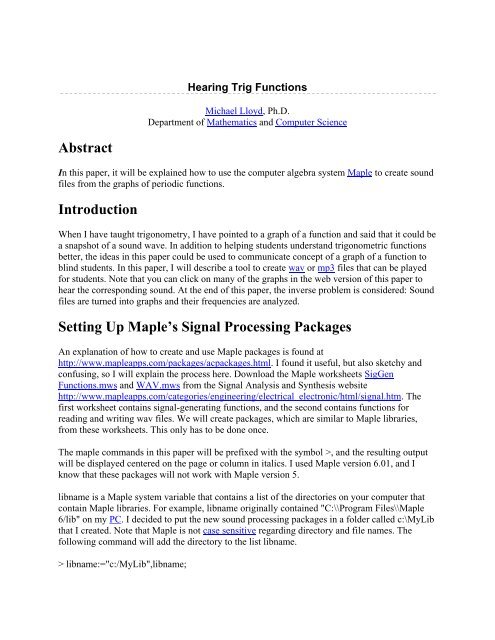
<strong>Hearing</strong> <strong>Trig</strong> <strong>Functions</strong><br />
Michael Lloyd, Ph.D.<br />
Department of Mathematics and Computer Science<br />
Abstract<br />
In this paper, it will be explained how to use the computer algebra system Maple to create sound<br />
files from the graphs of periodic functions.<br />
Introduction<br />
When I have taught trigonometry, I have pointed to a graph of a function and said that it could be<br />
a snapshot of a sound wave. In addition to helping students understand trigonometric functions<br />
better, the ideas in this paper could be used to communicate concept of a graph of a function to<br />
blind students. In this paper, I will describe a tool to create wav or mp3 files that can be played<br />
for students. Note that you can click on many of the graphs in the web version of this paper to<br />
hear the corresponding sound. At the end of this paper, the inverse problem is considered: Sound<br />
files are turned into graphs and their frequencies are analyzed.<br />
Setting Up Maple’s Signal Processing Packages<br />
An explanation of how to create and use Maple packages is found at<br />
http://www.mapleapps.com/packages/acpackages.html. I found it useful, but also sketchy and<br />
confusing, so I will explain the process here. Download the Maple worksheets SigGen<br />
<strong>Functions</strong>.mws and WAV.mws from the Signal Analysis and Synthesis website<br />
http://www.mapleapps.com/categories/engineering/electrical_electronic/html/signal.htm. The<br />
first worksheet contains signal-generating functions, and the second contains functions for<br />
reading and writing wav files. We will create packages, which are similar to Maple libraries,<br />
from these worksheets. This only has to be done once.<br />
The maple commands in this paper will be prefixed with the symbol >, and the resulting output<br />
will be displayed centered on the page or column in italics. I used Maple version 6.01, and I<br />
know that these packages will not work with Maple version 5.<br />
libname is a Maple system variable that contains a list of the directories on your computer that<br />
contain Maple libraries. For example, libname originally contained "C:\\Program Files\\Maple<br />
6/lib" on my PC. I decided to put the new sound processing packages in a folder called c:\MyLib<br />
that I created. Note that Maple is not case sensitive regarding directory and file names. The<br />
following command will add the directory to the list libname.<br />
> libname:="c:/MyLib",libname;
Execute the block of code (a module) at the top if the SigGen <strong>Functions</strong>.mws file. To create the<br />
package, do<br />
> savelib(SigGen);<br />
The signal generating function package now exists in memory, but it is not permanently stored<br />
on your hard drive until you do<br />
> march('create',libname[1],100);<br />
Now, repeat the process for the other Maple worksheet, WAV.mws. That is, execute the module<br />
block at the top of the WAV.mws file, and then do<br />
> savelib(WAV); march('create',libname[1],100);<br />
The second command will appear to generate the error:<br />
Error, (in march) there is already an archive in "C:/MyLib"<br />
However, Maple added the WAV package to the signal-generating package that you made<br />
earlier. The process I just described only needs to be completed once. However, when you come<br />
back another day and you want to access the functions in the two packages, you will need to tell<br />
Maple the directory you put them in:<br />
> libname:="c:/MyLib",libname;<br />
Then load the packages the same way you load commonly used libraries such as plots and linalg:<br />
> with(SigGen);<br />
[ASD, Attack, Decay, FM_Signal, FM_Sine, Integer2Bytes, LFO, Limiter, Normalize,<br />
Quantize, Sawtooth, Signal, Sine, ViewEnvelope, WriteSound, word2byte, writeintegers]<br />
> with(WAV);<br />
[ReadWAV, WriteWAV]<br />
A complete description of these signal-generating and wav functions will be found at the Maple<br />
Signal Analysis and Synthesis website referred to earlier.<br />
Simple Sine Wave<br />
Suppose we want to hear what a simple sine wave sounds like. The<br />
frequency obviously must be in the range of human hearing, so I choose<br />
440 Hertz, which is the standard frequency set for the A above middle C.
Of course, the actual formula for a simple sine wave with this frequency is ,<br />
but the shape will be the same. Also, we will not be concerned about the amplitude as long as we<br />
can hear the sound. The following Maple variables will remain the same for all the wav files we<br />
make:<br />
> Duration:=5: # Duration in seconds<br />
> SampleFreq:=44100: # full CD sample rate, number of samples per second<br />
> Resolution:=16: # 2^16 levels is CD quality, 2^8 is telephone<br />
> deltaT:=1/SampleFreq: # time between adjacent sample data<br />
> Npoints:=round(Duration*SampleFreq); # number of points in sample<br />
The number of points required to generate 5 seconds worth of sound at CD quality is<br />
. Consequently, each Maple command often takes several minutes to<br />
execute, even on my 650 MHz computer. The signal information is inputted as lists. You can add<br />
more sine waves to the signal if you like by extending these lists.<br />
> amps:=[1]: # list of amplitudes<br />
> freqs:=[440]: # list of frequencies<br />
Here is a plot of the first 0.01 seconds of the sound:<br />
> plot('Signal(amps,freqs,t)',t=0..0.01, title=”Simple Sine<br />
Wave\nClick to Hear”);<br />
The vertical axis is understood to be pressure, and the<br />
horizontal axis is time in seconds.<br />
I decided to use the function Signal from the SigGen package to keep in the spirit of signal<br />
processing instead of writing out the function in mathematical form. The next command will<br />
generate the data that will be converted to a wav:<br />
< p>>SigData:=Array([seq(Signal(amps,freqs,i*deltaT),i=1..Npoints)],datatype=float):<br />
The Array data type in Maple is similar to a list, except that by specifying the type of its<br />
elements to be float, Maple supposedly will process it faster. Here is the command for writing a<br />
wav file for this sound:<br />
> WriteWAV("c:/~temp/exams/sine440.wav", SigData, SampleFreq, Resolution);<br />
"Quantizing to 16 bits..."<br />
1 channel(s) found.<br />
220500 points per channel found.
"Saving to c:/~temp/exams/sine440.wav"<br />
"Done"<br />
You will get an IO error if a file with that name already exists. I stored these files in the directory<br />
C:/~temp/exams/, but you could store them in any directory that you like. The size of the wav<br />
file “sin.wav” was 430 kilobytes. I compressed it to an mp3 using the freeware, dBPowerAmp<br />
Music Convertor. The corresponding mp3 was 78.7 kilobytes which makes it more suitable for<br />
putting on a web page. In a previous talk, Math in Music, I used midi files exclusively. Midi files<br />
are much smaller than mp3s and wavs, and they are much faster to generate, but I was restricted<br />
to using a limited palette of sounds, and in fact, they may sound differently depending on the<br />
computer they are played on. By using wavs, you hear exactly what the sound looks like.<br />
Square, Saw Tooth, and Triangular Waves<br />
The simple waves which follow, are all the same note that was created above, only the timbre<br />
will be different. To save time and memory, I reused the same SigData variable name to create<br />
the data for a square wave:<br />
> SigData:=<br />
Array([seq(signum(SigData[i]),i=1..Npoints)],datatype=flo<br />
at):<br />
Here is the graph:<br />
> with(plots):<br />
> listplot([seq(SigData[i],i=1..441)],<br />
title="Square Wave\nClick to Hear");<br />
Note that the square corners require many frequencies, so that the<br />
frequency distribution appears fairly flat (Click to hear):<br />
I could hear the mp3 was not quite as good as the wav, and this is<br />
illustrated in its frequency distribution (Click to hear):
Here are the commands for generating plots for the sawtooth<br />
and triangular waves:<br />
> plot(Sawtooth(440,0,t),t=0..0.01, title="Saw Tooth<br />
Wave\nClick to Hear");<br />
> plot(abs(Sawtooth(440,0,t)-.5),t=0..0.01,<br />
title="Triangular Wave\nClick to Hear");<br />
An Almost Perfect Wave<br />
Most people find the simple waves shown above to be<br />
annoying. In the paper “Designing a Pleasing Sound<br />
Mathematically”, Erich Neuwirth said that the function<br />
sounds pleasing.<br />
is simple, yet<br />
> PleasingSound:=t->sin(2*Pi*440*t)/(1.25-<br />
cos(2*Pi*440*t));<br />
> plot(PleasingSound(t),t=0..0.01, title="A Pleasing<br />
Wave\nClick to Hear");<br />
Beats<br />
The musical phenomenon of beats occurs when two sounds with approximately the same<br />
frequencies combine. The volume of the sound can be heard to oscillate, and the frequency of<br />
this oscillation is called the beat frequency. When I teach trigonometry, I work an example<br />
involving beats where a sum-to-product identity is applied. The beat frequency will be the<br />
difference of the two component frequencies, and the perceived pitch of the combined notes will<br />
be the average of the two pitches. String players often tune their instruments using the concept of
eats: They simply adjust the string tension until the beats disappear.<br />
I decided to use the frequencies 440 Hz and 441 Hz:<br />
> amps:=[1,1]: freqs:=[440,441]:<br />
The beat frequency is<br />
and the<br />
perceived frequency is<br />
is a plot of the first 2.5 seconds of the sound.<br />
. Here<br />
> plot('Signal(amps,freqs,t)',t=0..2.5, title="Beats\nClick<br />
to Hear");<br />
Note that there are about 440 oscillations squished into each lobe, so a complete graph would<br />
appear solid.<br />
Envelopes<br />
The boundary around the graph of the beats above is called an<br />
envelope. This suggests a method for “hearing” nontrigonometric<br />
curves. For example, suppose you wanted to<br />
“hear” the parabola :<br />
The essence of the shape stays the same if we translate the<br />
parabola horizontally, so I decided to put the vertex in the<br />
middle of a 5 second 440 Hz sine wave.<br />
> amps:=[1]: freqs:=[440]:<br />
> SigData:= Array([seq((i*deltaT-<br />
2.5)^2*Signal(amps,freqs,i*deltaT),i=1..Npoints)],datatype=<br />
float):<br />
> plot('(t-2.5)^2*Signal(amps,freqs,t)',t=0..5,<br />
title="Parabolic Envelope\nClick to Hear);<br />
Unfortunately, you cannot tell from this sound whether the function is above or below the x-axis.<br />
The Maple signal-processing commands do allow the creation of stereo wave files, so one
solution to this dilemma would be to put the sound through the left channel if the function were<br />
negative, and put it through the right, if the function were positive. For example, suppose we<br />
wanted to hear the graph of the cubic . The commands for creating the stereo sound<br />
appear below. Creating the array took 1 hour and writing the 5-second stereo wav file took<br />
8.5 hours on my 450 MHz PC! Click here or on the far left graph of the cubic to hear the stereo<br />
sound.<br />
> stereo:=t->[piecewise(t2.5,(t-<br />
2.5)^3*Signal(amps,freqs,t),0)]:<br />
>SigData:=Array([seq(stereo(i*deltaT),i=1..Npoints))],datatype=float):<br />
> WriteWAV("c:/~temp/exams/cubic.wav", SigData2, SampleFreq, Resolution);2 channel(s)<br />
found.<br />
220500 points per channel found.<br />
"Interweaving sound data..."<br />
Combining <strong>Trig</strong>onometric <strong>Functions</strong><br />
For the first example below, I made the amplitudes the same, and used a Maple function called<br />
chord. This function generates a list of frequencies if you tell it the names of the notes and<br />
octaves to which these notes belong. A complete description of this function and its listing are<br />
given in the appendix. The two notes in this example are an octave apart, that is, the higher<br />
frequency is twice the other. The shape of the graph is the same as the graph of the function<br />
.
amps:=[1,1]: freqs:=chord(["A","A"],[4,5]);<br />
freqs := [440.00, 880.00]<br />
A major chord is generated for this second<br />
example. This graph is close to the graph<br />
of .<br />
> amps:=[1,1,1]:<br />
> freqs:=chord(["C","E","G"],[4,4,4]);<br />
freqs := [261.6255653, 329.6275568, 391.9954358]<br />
For the third example, the<br />
middle note is dropped half<br />
of a step to form a C minor<br />
chord. This graph is close to<br />
the graph of<br />
.<br />
> freqs:=chord(["C","Eb","G"],[4,4,4]);<br />
freqs := [261.6255653, 311.1269838, 391.9954358]<br />
It is not clear by looking at the graphs of these pressure-versus-time plots why a major chord is<br />
more consonant than a minor chord. I believe that the right way to visualize a complex sound is<br />
to look at a frequency distribution. According to the resonance theory of hearing, our ears acts<br />
like a Fourier transform by separating the sound into its component frequencies before sending<br />
the signals to our brain. The major chord is more consonant because the frequencies that make<br />
up that sound are roughly proportional to smaller integers.
Analyzing CBL Data<br />
The following Maple commands create a buffer for reading in pressure data. This data was<br />
obtained by playing a guitar string into a microphone attached to a Calculator Based Laboratory<br />
(CBL) like the one pictured here.<br />
> fd := fopen(`C:/~temp/exams/FFTpress.txt`,READ,TEXT):<br />
> InData:=readdata(fd, float):<br />
> fclose(fd):<br />
> InDataSize:=nops(InData);<br />
InDataSize := 32<br />
We will do a Fast Fourier Transform (FFT) on this data to compute the component frequencies.<br />
The original data contained 99 time-pressure pairs of data. (99 is the largest dimension for a list<br />
on the TI-82 graphing calculator.) Since the FFT requires that the data size be a power of 2, I<br />
applied linear interpolation to the original data to get exactly 32 points for one cycle of the<br />
sound. For thousands of points, it is unnecessary to do this interpolation or get an integral<br />
number of cycles, just take the largest power of 2 points. Here is a graph of the cycle that I<br />
chose:<br />
> listplot([seq(InData[k][1],k=1..InDataSize)], title="D String");<br />
The following Maple commands are used to set up the FFT:<br />
> m:=5: SigSize:=2^m;<br />
SigSize := 32<br />
> RealPart:=hfarray([seq(InData[i][1],<br />
i=1..SigSize)]):<br />
>ImagPart:=hfarray([seq(0,i=1..SigSize)]):<br />
Now to perform the FFT:<br />
> evalhf(FFT(m,RealPart,ImagPart)):
The hardware float arrays RealPart and ImagPart now contain the complex frequencies. We will<br />
use the following Maple function to find the real magnitude for each frequency:<br />
> mag:=proc(RealPart, ImagPart): sqrt(RealPart^2+ImagPart^2): end:<br />
The sample period 000210266 in units of seconds was manually obtained from the time text file.<br />
> SampleFreq:=1/.000210266;<br />
SampleFreq := 4755.880646<br />
The variable df (delta frequency) is a scaling factor that relates the indices of the RealPart and<br />
ImagPart arrays to the actual frequency.<br />
> df:=evalf(SampleFreq/SigSize):<br />
> FreqSpectrum:= [seq([(i-<br />
1)*df,(2*mag(RealPart[i],ImagPart[i])/SigSize)],i=1..floor((SigSize/2)))]:<br />
Here is a plot of the frequency spectrum:<br />
> listplot([seq(FreqSpectrum[i],i=1..10)],<br />
title="Frequency Spectrum");<br />
The two peaks are<br />
> FreqSpectrum[2];FreqSpectrum[7];<br />
[148.6212702, .03009241976]<br />
[891.7276212, .001030763241]<br />
A useful feature in Maple is that you can left click on a graph and read the coordinates. Doing<br />
that and then looking at the list, we see that the peaks are at approximately 149 Hz and 892 Hz. If<br />
the data set had been much larger, then these peaks would be very narrow. 149 Hz is close to the<br />
note D (146.8 Hz), and 892 Hz is close to the note A (880 Hz), the harmonic which is about 6<br />
times higher. I generated the sound by plucking the D string in the middle, which explains the<br />
lack of the harmonics 2 through 5. If I had used a pick near the bridge and the data set had been<br />
much larger, these other harmonics should have been visible.<br />
Analyzing WAV Data<br />
In this section, we will analyze a wav file that I created by connecting a tape player to my sound<br />
card. I trimmed the file using the software GoldWave. This wav is the sung word, “wonderful”<br />
(click to hear) in a song called “Cornerstone”. At this point in the song, the pianist at our church<br />
and I disagreed on the chord accompaniment. She believed the chord to be minor while I
elieved the chord should be major. We will do a spectral analysis on this wav to determine who<br />
was correct.<br />
The first step is to make sure that the variable SampleFreq is free.<br />
> SampleFreq:='SampleFreq':<br />
The function ReadWAV will pass the sample frequency to its second argument.<br />
> SigData:=ReadWAV("c:/~temp/exams/wavs/wonderful.wav",SampleFreq):<br />
> SampleFreq;<br />
44100<br />
Here are three graphs of the sampled sound to demonstrate its appearance at various time scales:<br />
The Maple command ArrayNumElems(SigData) gives 80970 for the sample size, so we will use<br />
the first<br />
points for the FFT. A graph of the frequency spectrum appears here.<br />
The frequencies for the two highest peaks in Hertz are 125 Hz and 254 Hz, clearly an octave<br />
apart. These notes are close to a B, which I will take to be the root of the appropriate chord for<br />
the sampled portion of the song.<br />
I decided not to include the Maple commands which were used to generate the remaining plots<br />
for this paper because they were a bit tedious. Many of the commands were tedious and some are<br />
at the website. Each graph shows the original frequency spectrum on the bottom. The downward<br />
pointing spikes for the first graph locate the powers of 2 times the root frequency 254 Hz. The<br />
next two graphs compare the original frequency spectrum with the powers of 2 multiples of the<br />
major and minor 3 rd , respectively. (A major 3 rd above 254 Hz is computed ; a minor 3 rd above<br />
254 Hz is computed .)<br />
The major 3 rds (the middle graph) matches better than the minor 3 rds (the last graph), so a B major<br />
chord is a better fit than B minor.
I made an animation of the frequency spectrum evolving over time, but the sample size was only<br />
large enough to make 4 time frames. Each frame pictured here is 0.37 seconds apart.<br />
The waterfall plot is another way to visualize the frequencies evolving over time. The row axis is<br />
time (slice 1, 2, 3, and 4); the column axis is frequency (Hz).<br />
If the waterfall plot is turned on end, then the Looking at the other end, you can see how the<br />
graph is almost the same as the original wav is getting quieter over time. (Increasing<br />
frequency spectrum.<br />
time is right to left.)<br />
Appendix: Maple Function for Generating Chord<br />
Frequencies<br />
Author: Michael Lloyd Date: August 2001<br />
Description<br />
This function takes a sequence of notes and corresponding octaves and returns a frequency list to<br />
be used by the functions in the SigGen Maple package. The 0th octave corresponds to the lowest<br />
notes on a piano, and the 4th octave is middle C up to and including the B on the treble clef.<br />
(This is the octave identification system recommended by the International Acoustical Society<br />
and also used in Braille music notation.) For example, a command for generating the frequencies<br />
for a C chord is chord(["C","E","G"],[4,4,4]); This will return the list [261.6255653,<br />
329.6275568, 391.9954358] where each frequency is in Hertz.<br />
This function can be improved by adding enharmonic notes that require double sharps or double<br />
flats such as “FX” or “Ebb”. This would accommodate musically correct spellings of the chords<br />
in unusual keys or chords such as Ab diminished which should be spelled as Ab Cb Ebb.<br />
Program Listing<br />
chord := proc(notes, octaves)
local freqs, k, scale;<br />
freqs := NULL;<br />
for k to nops(notes)<br />
do<br />
if notes[k] = "C" or notes[k] = "B#" then scale := 0 end if;<br />
if notes[k] = "C#" or notes[k] = "Db" then scale := 1 end if;<br />
if notes[k] = "D" then scale := 2 end if;<br />
if notes[k] = "D#" or notes[k] = "Eb" then scale := 3 end if;<br />
if notes[k] = "E" or notes[k] = "Fb" then scale := 4 end if;<br />
if notes[k] = "F" or notes[k] = "E#" then scale := 5 end if;<br />
if notes[k] = "F#" or notes[k] = "Gb" then scale := 6 end if;<br />
if notes[k] = "G" then scale := 7 end if;<br />
if notes[k] = "G#" or notes[k] = "Ab" then scale := 8 end if;<br />
if notes[k] = "A" then scale := 9 end if;<br />
if notes[k] = "A#" or notes[k] = "Bb" then scale := 10 end if;<br />
if notes[k] = "B" or notes[k] = "Cb" then scale := 11 end if;<br />
freqs := freqs, 13.75*2^(octaves[k] + 1/12*scale + .25)<br />
end do;<br />
freqs := [freqs]<br />
end proc<br />
References
Creating Maple 6 Library Packages, http://www.mapleapps.com/packages/acpackages.html.<br />
“Designing a Pleasing Sound Mathematically” by Erich Neuwirth, Mathematics Magazine,<br />
Vol. 74, No. 2, April 2001, pp. 91-98.<br />
"Music in Theory and Practice" by Bruce Benward and Gary White ©1989 WmC Brown<br />
Publishing Co.<br />
Signal Analysis and Synthesis,<br />
http://www.mapleapps.com/categories/engineering/electrical_electronic/html/signal.htm.<br />
Software Used in This Paper<br />
dBPowerAmp (music convertor), http://admin.dbpoweramp.com/<br />
GoldWave (digital audio editor), http://www.goldwave.com/<br />
Maple version 6.01 (computer algebra system), http://www.maplesoft.com<br />
Microsoft Photo Editor<br />
Noteworthy Composer (music composer), http://www.NoteworthyComposer.com<br />
NullSoft WinAmp (mp3 player), http://www.winamp.com/<br />
Biographical Sketch<br />
Michael Lloyd received his B.S in Chemical Engineering in 1984 and his Ph.D. in Mathematics<br />
from Kansas <strong>State</strong> <strong>University</strong> in Manhattan. He has presented papers at meetings of the<br />
Mathematical Association of America, the Arkansas Conference on Teaching, and the American<br />
Mathematical Society. He has been at <strong>Henderson</strong> <strong>State</strong> <strong>University</strong> since August 1993.<br />
Disclaimer: <strong>Henderson</strong> <strong>State</strong> <strong>University</strong> and the Office of Computer and Communication Services assume no responsibility for any information or representations contained in the<br />
student/faculty/alumni web pages. These web pages and any opinions, information or representations contained therein are the creation of the particular individual or organization and do not<br />
necessarily reflect the opinion of <strong>Henderson</strong> <strong>State</strong> <strong>University</strong> or its Office of Computer and Communication Services. All individuals publishing materials on the <strong>Henderson</strong> <strong>State</strong> <strong>University</strong> Web<br />
Server understand that the submission, installation, copying, distribution, and use of such materials in connection with the Web Server will not violate any other party's proprietary rights.


