Ensemble Classification for Spam Filtering Based on Clustering of ...
Ensemble Classification for Spam Filtering Based on Clustering of ...
Ensemble Classification for Spam Filtering Based on Clustering of ...

You also want an ePaper? Increase the reach of your titles
YUMPU automatically turns print PDFs into web optimized ePapers that Google loves.
<str<strong>on</strong>g>Ensemble</str<strong>on</strong>g> <str<strong>on</strong>g>Classificati<strong>on</strong></str<strong>on</strong>g> <str<strong>on</strong>g>for</str<strong>on</strong>g> <str<strong>on</strong>g>Spam</str<strong>on</strong>g> <str<strong>on</strong>g>Filtering</str<strong>on</strong>g><br />
<str<strong>on</strong>g>Based</str<strong>on</strong>g> <strong>on</strong> <strong>Clustering</strong> <strong>of</strong> Text Corpora<br />
Robert Neumayer<br />
neumayer@tcd.ie<br />
Visiting Student<br />
Final Year Project 2006<br />
Supervisor: Dr. Pádraig Cunningham
C<strong>on</strong>tents<br />
1 Introducti<strong>on</strong> 1<br />
1.1 General Objectives . . . . . . . . . . . . . . . . . . . . . . . . . . 2<br />
1.2 Synopsis . . . . . . . . . . . . . . . . . . . . . . . . . . . . . . . . 2<br />
2 Related Work 3<br />
2.1 Supervised Machine Learning . . . . . . . . . . . . . . . . . . . . 4<br />
2.1.1 k-Nearest Neighbour Classifiers . . . . . . . . . . . . . . . 4<br />
2.2 Unsupervised Machine Learning . . . . . . . . . . . . . . . . . . . 4<br />
2.2.1 k-Means <strong>Clustering</strong> . . . . . . . . . . . . . . . . . . . . . . 5<br />
2.2.2 Self-Organizing Map . . . . . . . . . . . . . . . . . . . . . 5<br />
2.2.3 <str<strong>on</strong>g>Ensemble</str<strong>on</strong>g> <str<strong>on</strong>g>Classificati<strong>on</strong></str<strong>on</strong>g> . . . . . . . . . . . . . . . . . . . 5<br />
2.3 Objectives Revisited . . . . . . . . . . . . . . . . . . . . . . . . . 7<br />
3 Text Categorisati<strong>on</strong> and Text In<str<strong>on</strong>g>for</str<strong>on</strong>g>mati<strong>on</strong> Retrieval 8<br />
3.1 Applicati<strong>on</strong> Scenario . . . . . . . . . . . . . . . . . . . . . . . . . 9<br />
3.2 Per<str<strong>on</strong>g>for</str<strong>on</strong>g>mance Measurements . . . . . . . . . . . . . . . . . . . . . 9<br />
3.3 Database Implementati<strong>on</strong> . . . . . . . . . . . . . . . . . . . . . . 10<br />
4 Feature Selecti<strong>on</strong> and Dimensi<strong>on</strong>ality Reducti<strong>on</strong> 12<br />
4.0.1 In<str<strong>on</strong>g>for</str<strong>on</strong>g>mati<strong>on</strong> Gain . . . . . . . . . . . . . . . . . . . . . . . 12<br />
4.0.2 Odds Ratio . . . . . . . . . . . . . . . . . . . . . . . . . . 13<br />
4.1 Combinati<strong>on</strong> <strong>of</strong> Feature Selecti<strong>on</strong> Approaches . . . . . . . . . . . 13<br />
4.1.1 Feature Selecti<strong>on</strong> Experiments . . . . . . . . . . . . . . . 13<br />
4.1.2 Document Frequency Thresholding . . . . . . . . . . . . . 14<br />
5 Ensemles <strong>of</strong> Classifiers <str<strong>on</strong>g>for</str<strong>on</strong>g> <str<strong>on</strong>g>Spam</str<strong>on</strong>g> <str<strong>on</strong>g>Classificati<strong>on</strong></str<strong>on</strong>g> 16<br />
5.1 Experimental Setup . . . . . . . . . . . . . . . . . . . . . . . . . 16<br />
5.2 Preprocessing . . . . . . . . . . . . . . . . . . . . . . . . . . . . . 17<br />
5.3 <str<strong>on</strong>g>Classificati<strong>on</strong></str<strong>on</strong>g> Experiments . . . . . . . . . . . . . . . . . . . . . . 17<br />
5.3.1 k-NN . . . . . . . . . . . . . . . . . . . . . . . . . . . . . 17<br />
5.3.2 Decisi<strong>on</strong> Functi<strong>on</strong> . . . . . . . . . . . . . . . . . . . . . . 18<br />
5.3.3 <str<strong>on</strong>g>Ensemble</str<strong>on</strong>g> <str<strong>on</strong>g>Classificati<strong>on</strong></str<strong>on</strong>g> . . . . . . . . . . . . . . . . . . . 18<br />
5.3.4 Less<strong>on</strong>s Learned from the First Shot . . . . . . . . . . . . 19<br />
5.4 New Winner Take All Strategy . . . . . . . . . . . . . . . . . . . 21<br />
1
5.4.1 Aggregati<strong>on</strong> Technique Revisited . . . . . . . . . . . . . . 21<br />
6 <strong>Clustering</strong> <strong>of</strong> the TREC <str<strong>on</strong>g>Spam</str<strong>on</strong>g> Corpus 23<br />
6.1 Cluster Validati<strong>on</strong> Techniques: Silhouette Value . . . . . . . . . . 23<br />
6.2 Cluster Validati<strong>on</strong> <strong>of</strong> the Self-Organizing Map . . . . . . . . . . . 24<br />
6.3 Finally: Subsampling <strong>of</strong> the TREC Corpus . . . . . . . . . . . . 25<br />
7 C<strong>on</strong>clusi<strong>on</strong>s and Future Work 28<br />
8 Acknowledgements 30<br />
2
Abstract<br />
<str<strong>on</strong>g>Spam</str<strong>on</strong>g> filtering has become a very important issue throughout the last years as<br />
unsolicited bulk e-mail imposes large problems in terms <strong>of</strong> both the amount <strong>of</strong><br />
time spent <strong>on</strong> and the resources needed to automatically filter those messages.<br />
Text in<str<strong>on</strong>g>for</str<strong>on</strong>g>mati<strong>on</strong> retrieval <strong>of</strong>fers the tools and algorithms to handle text documents<br />
in their abstract vector <str<strong>on</strong>g>for</str<strong>on</strong>g>m. There<strong>on</strong>, machine learning algorithms<br />
can be applied. This work deals with the possible improvements gained from<br />
ensembles, i.e. multiple, differing classifiers <str<strong>on</strong>g>for</str<strong>on</strong>g> the same task. Those individual<br />
classifiers can fit parts <strong>of</strong> the training data better and there<str<strong>on</strong>g>for</str<strong>on</strong>g>e may<br />
improve classificati<strong>on</strong> results, when the best fitting classifier can be found. Basic<br />
classificati<strong>on</strong> algorithms as well as clustering are introduced. Furthermore<br />
the applicati<strong>on</strong> <strong>of</strong> the ensemble idea is explained and experimental results are<br />
presented.
Chapter 1<br />
Introducti<strong>on</strong><br />
Unsolicited commercial e-mail has become a serious problem <str<strong>on</strong>g>for</str<strong>on</strong>g> both private<br />
and commercial e-mail users. By now, spam is estimated to be a very high<br />
percentage <strong>of</strong> all e-mail traffic (in some estimates up to 80 % or even more).<br />
The resulting waste <strong>of</strong> resources (hardware, time, etc.) is enormous.<br />
The currently employed infrastructure <str<strong>on</strong>g>for</str<strong>on</strong>g> e-mail transfer, the simple mail<br />
transfer protocol (SMTP), hardly provides any support <str<strong>on</strong>g>for</str<strong>on</strong>g> detecting or preventing<br />
spam. We are also lacking a widely accepted and deployed authenticati<strong>on</strong><br />
mechanism <str<strong>on</strong>g>for</str<strong>on</strong>g> the sending <strong>of</strong> e-mails. Thus, until a new global e-mail infrastructure<br />
has been developed which allows <str<strong>on</strong>g>for</str<strong>on</strong>g> better c<strong>on</strong>trolling <strong>of</strong> this problem,<br />
two major approaches show the greatest potential <str<strong>on</strong>g>for</str<strong>on</strong>g> coping with the problem:<br />
detecting spam based <strong>on</strong> c<strong>on</strong>tent filtering or preventing spam based <strong>on</strong><br />
increasing the costs associated with sending out e-mail messages.<br />
This work c<strong>on</strong>centrates <strong>on</strong> the applicati<strong>on</strong> <strong>of</strong> machine learning techniques<br />
to the spam problem and there<str<strong>on</strong>g>for</str<strong>on</strong>g>e clearly bel<strong>on</strong>gs to the c<strong>on</strong>tent filtering category.<br />
The main task <strong>of</strong> machine learning is to “learn” labels <strong>of</strong> instances (like<br />
legitimate or n<strong>on</strong>-legitimate <str<strong>on</strong>g>for</str<strong>on</strong>g> e-mail messages) from a given training set, and<br />
subsequently tag new or unknown instances (e.g. incoming e-mails).<br />
More specifically, the feasibility <strong>of</strong> decomposing spam training sets into<br />
smaller, more specialised subsets <str<strong>on</strong>g>for</str<strong>on</strong>g> spam filtering is investigated. The main<br />
idea behind this is that the similarity <strong>of</strong> incoming messages to all those subsets<br />
can be computed, <strong>on</strong>e <strong>of</strong> which the message is likely to fit in best. That subset<br />
can then be used to label that specific instance. There<str<strong>on</strong>g>for</str<strong>on</strong>g>e, the ensemble classificati<strong>on</strong><br />
approach was chosen. Usually, <strong>on</strong>e classifier is built <strong>on</strong> <strong>on</strong>e training set,<br />
and this classifier is then used to categorise incoming messages. <str<strong>on</strong>g>Ensemble</str<strong>on</strong>g>s comprise<br />
several classifiers <str<strong>on</strong>g>for</str<strong>on</strong>g> the same task, varying either in parameter settings<br />
or data used <str<strong>on</strong>g>for</str<strong>on</strong>g> training. This work relies <strong>on</strong> the latter type <strong>of</strong> ensemble.<br />
1
1.1 General Objectives<br />
The goal <strong>of</strong> this work is to prove that exploiting the diversity am<strong>on</strong>gst spam and<br />
ham messages and the use <strong>of</strong> multiple classifiers based <strong>on</strong> those subgroups can<br />
outper<str<strong>on</strong>g>for</str<strong>on</strong>g>m <strong>on</strong>e single classifier in terms <strong>of</strong> classificati<strong>on</strong> accuracy. The primary<br />
purpose is to show the applicability <strong>of</strong> ensemble techniques to the spam problem,<br />
particularly in how far different aggregati<strong>on</strong> techniques to combine the results<br />
<strong>of</strong> several classifiers are feasible in this scenario. Moreover, the issue <strong>of</strong> classifier<br />
c<strong>on</strong>fidence, i.e. how c<strong>on</strong>fident a classifier is that his decisi<strong>on</strong> is the right <strong>on</strong>e,<br />
will be addressed.<br />
1.2 Synopsis<br />
The remainder <strong>of</strong> this report is structured as follows. Chapter 2 gives an<br />
overview <strong>of</strong> previous research, Chapter 3 introduces the main principles <strong>of</strong> text<br />
categorisati<strong>on</strong> and the applicati<strong>on</strong> <strong>of</strong> machine learning techniques. Furthermore,<br />
Chapter 3 deals with the problem <strong>of</strong> feature selecti<strong>on</strong> in the c<strong>on</strong>text <strong>of</strong> text in<str<strong>on</strong>g>for</str<strong>on</strong>g>mati<strong>on</strong><br />
retrieval. The applicati<strong>on</strong> <strong>of</strong> ensemble techniques to the spam problem<br />
is explained in Chapter 5. Chapter 6 gives an overview about clustering and<br />
experimental results. Finally, Chapter 7 gives a short outlook and summarises<br />
the work d<strong>on</strong>e.<br />
2
Chapter 2<br />
Related Work<br />
Numerous spam filtering strategies with varying degrees <strong>of</strong> efficiency have been<br />
proposed and developed. Many <strong>of</strong> them implement static or rule based approaches,<br />
which leave opportunities <str<strong>on</strong>g>for</str<strong>on</strong>g> spammers to react and circumvent existing<br />
anti-spam soluti<strong>on</strong>s. As a result, many <strong>of</strong> the existing approaches yield<br />
good classificati<strong>on</strong> results <strong>on</strong>ly over short periods <strong>of</strong> time (until spammers have<br />
found a workaround). This aspect manifests itself in an <strong>on</strong>going “arms race” between<br />
spammers and developers <strong>of</strong> spam filtering s<strong>of</strong>tware. The most important<br />
and the most widespread example <str<strong>on</strong>g>for</str<strong>on</strong>g> such an approach is Apache’s <str<strong>on</strong>g>Spam</str<strong>on</strong>g>Assassin<br />
[1], currently a de-facto standard <str<strong>on</strong>g>for</str<strong>on</strong>g> e-mail classificati<strong>on</strong> and spam filtering.<br />
Here, a large number (currently over 700) <strong>of</strong> many different types <strong>of</strong> tests and<br />
checks are combined. In this case the decisi<strong>on</strong> whether a message is spam or<br />
not is based <strong>on</strong> a simple thresholding mechanism. The weightings <str<strong>on</strong>g>for</str<strong>on</strong>g> the different<br />
tests are computed by a linear perceptr<strong>on</strong> based up<strong>on</strong> large spam and ham<br />
corpora. Bey<strong>on</strong>d that, many other products and tools have been developed <str<strong>on</strong>g>for</str<strong>on</strong>g><br />
spam filtering (both commercial and open source). Although they may have<br />
different names, they <strong>of</strong>ten rely <strong>on</strong> similar methods, and some are even directly<br />
based <strong>on</strong> <str<strong>on</strong>g>Spam</str<strong>on</strong>g>Assassin.<br />
More generally, by omitting the special nature <strong>of</strong> e-mail traffic, spam filtering<br />
can be regarded as a classic text categorisati<strong>on</strong> task. Thorough research has been<br />
c<strong>on</strong>ducted in this field.<br />
Machine learning techniques are widely used in automated text classificati<strong>on</strong>,<br />
including spam filtering (see [2] <str<strong>on</strong>g>for</str<strong>on</strong>g> a survey <strong>of</strong> techniques used). Due to<br />
their simplicity and per<str<strong>on</strong>g>for</str<strong>on</strong>g>mance advantages over many other sophisticated approaches<br />
naïve Bayes classifiers [3] are maybe the most prevalent. They have<br />
been used <str<strong>on</strong>g>for</str<strong>on</strong>g> spam filtering with great success, since <strong>on</strong>line training is particularly<br />
well supported. Many implementati<strong>on</strong>s are available, most <strong>of</strong> them based<br />
<strong>on</strong> Paul Graham’s ideas [4, 5]. Case-based techniques, c<strong>on</strong>centrating <strong>on</strong> editing<br />
the case base and counteracting c<strong>on</strong>cept drift in spam mails, are described<br />
in [6]. [7] shows that n-gram frequencies do not necessarily boost classificati<strong>on</strong><br />
per<str<strong>on</strong>g>for</str<strong>on</strong>g>mance in the spam c<strong>on</strong>text as well as the importance <strong>of</strong> meta data <str<strong>on</strong>g>for</str<strong>on</strong>g> this<br />
task.<br />
3
In terms <strong>of</strong> classifier techniques, the feasibility <strong>of</strong> applying support vector<br />
machines (SVM) <str<strong>on</strong>g>for</str<strong>on</strong>g> text classificati<strong>on</strong> has been investigated in [8]. The use<br />
<strong>of</strong> latent semantic indexing (LSI) <str<strong>on</strong>g>for</str<strong>on</strong>g> spam filtering is assessed in [9]. A comprehensive<br />
comparis<strong>on</strong> <strong>of</strong> different text categorisati<strong>on</strong> methods is also described<br />
in [10]. A k-NN classifier is compared to different LSI variants and support<br />
vector machines. SVMs and a k-NN supported LSI per<str<strong>on</strong>g>for</str<strong>on</strong>g>med best, all <strong>of</strong> which<br />
having both advantages and disadvantages.<br />
2.1 Supervised Machine Learning<br />
The main task in classificati<strong>on</strong> or supervised learning is to train a system <strong>on</strong><br />
a given labelled training set and then assign unknown instances to <strong>on</strong> <strong>of</strong> those<br />
labels. For the e-mail scenario that means, a known set <strong>of</strong> legitimate as well as<br />
n<strong>on</strong>-legitimate e-mails are used to train a classifier, the in<str<strong>on</strong>g>for</str<strong>on</strong>g>mati<strong>on</strong> taken from<br />
those labelled messages is then later used when new and unknown messages<br />
come in. How exactly that works depends <strong>on</strong> the algorithm used. The k nearest<br />
neighbour algorithm is <strong>on</strong>e <strong>of</strong> the simplest machine learning techniques, yet it<br />
is quite a powerful <strong>on</strong>e and will be used as classificati<strong>on</strong> technique throughout<br />
this report.<br />
2.1.1 k-Nearest Neighbour Classifiers<br />
k-NN compares a given query to all vectors in the training set and assigns the<br />
query to the class that the majority <strong>of</strong> the k most similar vectors are assigned to.<br />
Similarity in this c<strong>on</strong>text can be computed by a range <strong>of</strong> distance measurements,<br />
<strong>of</strong> which the Euclidean distance is the most comm<strong>on</strong>. k-NN classifiers bel<strong>on</strong>g<br />
to the category <strong>of</strong> so called lazy learners, i.e. all computati<strong>on</strong>al resources are<br />
needed at classificati<strong>on</strong> time. Its training phase is involves merely the storage<br />
<strong>of</strong> the training set as opposed to other algorithms like back-propagati<strong>on</strong> neural<br />
networks.<br />
Each query is compared to every single stored instance. Now the k closest<br />
instances in the training set are determined and the query is assigned to the<br />
prevailing class <strong>of</strong> those neighbours. If, <str<strong>on</strong>g>for</str<strong>on</strong>g> example, the three closest instances<br />
to a query are all labelled spam, the query message is labelled spam as well.<br />
The c<strong>on</strong>fidence <strong>of</strong> the 3-NN classifier would be 1.0, but could be .66 if <strong>on</strong>ly two<br />
out <strong>of</strong> the three neighbours would be spam.<br />
2.2 Unsupervised Machine Learning<br />
Unsupervised learning denotes the partiti<strong>on</strong>ing <strong>of</strong> a data set into subsets that<br />
c<strong>on</strong>tain similar elements in terms <strong>of</strong> a distance functi<strong>on</strong>. <strong>Clustering</strong> does not<br />
need class labels as the partiti<strong>on</strong>ing is d<strong>on</strong>e based <strong>on</strong> the data vectors <strong>on</strong>ly. In<br />
this c<strong>on</strong>text, clustering is used to partiti<strong>on</strong> existing ham and spam sets into<br />
subgroups.<br />
4
2.2.1 k-Means <strong>Clustering</strong><br />
k-Means clustering is a rather simple and well known technique. The input<br />
<str<strong>on</strong>g>for</str<strong>on</strong>g> the algorithm is a possibly unlabelled data set and a number <strong>of</strong> clusters to<br />
partiti<strong>on</strong> the data into. For each cluster, a centre vector is randomly initialised.<br />
Each data point is then assigned to the closest cluster centre. Then the new<br />
cluster centres are computed as the average over all data points assigned to each<br />
cluster. This is repeated until there are no more changes in cluster assignments.<br />
This technique was not actually used <str<strong>on</strong>g>for</str<strong>on</strong>g> any experiments, but is menti<strong>on</strong>ed<br />
to introduce the general clustering idea as well as to point out the differences<br />
between this algorithm and the Self-Organizing Map that is introduced in the<br />
next secti<strong>on</strong>.<br />
2.2.2 Self-Organizing Map<br />
The Self-Organizing Map, an unsupervised neural network that provides a mapping<br />
from a high-dimensi<strong>on</strong>al input space to usually two-dimensi<strong>on</strong>al output<br />
space was used <str<strong>on</strong>g>for</str<strong>on</strong>g> clustering [11, 12]. During that process topological relati<strong>on</strong>s<br />
are preserved as faithfully as possible. A SOM c<strong>on</strong>sists <strong>of</strong> a set <strong>of</strong> i units arranged<br />
in a two-dimensi<strong>on</strong>al grid, each attached to a weight vector m i ∈ R n .<br />
Elements from the high-dimensi<strong>on</strong>al input space, referred to as input vectors<br />
x ∈ R n , are presented to the SOM and the activati<strong>on</strong> <strong>of</strong> each unit <str<strong>on</strong>g>for</str<strong>on</strong>g> the<br />
presented input vector is calculated using an activati<strong>on</strong> functi<strong>on</strong> (usually the<br />
Euclidean Distance). In the next step the weight vector <strong>of</strong> the unit showing the<br />
highest activati<strong>on</strong> is modified as to more closely resemble the presented input<br />
vector. Subsequently, the weight vector <strong>of</strong> the winner is moved towards the presented<br />
input signal by a certain fracti<strong>on</strong> <strong>of</strong> the Euclidean distance as indicated<br />
by a time-decreasing learning rate α. C<strong>on</strong>sequently, the next time the same input<br />
signal is presented, this unit’s activati<strong>on</strong> will be even higher. Furthermore,<br />
the weight vectors <strong>of</strong> units neighbouring the winner, as described by a timedecreasing<br />
neighbourhood functi<strong>on</strong>, are modified accordingly, yet to a smaller<br />
amount as compared to the winner. Figure 2.1 shows that data points x can be<br />
assigned to different weight vectors m over time. This behaviour is particularly<br />
influenced by the learning rate and neighbouring functi<strong>on</strong>. The result <strong>of</strong> this<br />
learning procedure is a topologically ordered mapping <strong>of</strong> the presented input<br />
signals in two-dimensi<strong>on</strong>al space. Accordingly, similar input data are mapped<br />
<strong>on</strong>to neighbouring regi<strong>on</strong>s <strong>of</strong> the map.<br />
2.2.3 <str<strong>on</strong>g>Ensemble</str<strong>on</strong>g> <str<strong>on</strong>g>Classificati<strong>on</strong></str<strong>on</strong>g><br />
<str<strong>on</strong>g>Ensemble</str<strong>on</strong>g>s are groups <strong>of</strong> machine learning instances that work together and<br />
are used to improve the classificati<strong>on</strong> results <strong>of</strong> the overall system. The most<br />
popular <strong>on</strong>es are boosting and bagging [13]. Those algorithms train classifier<br />
instances <strong>on</strong> different subsets <strong>of</strong> the overall data set. Bagging combines the<br />
results <strong>of</strong> classifiers trained <strong>on</strong> sub samplings <strong>of</strong> the data set. A good overview<br />
<strong>of</strong> different ways <strong>of</strong> c<strong>on</strong>structing ensembles as well as an explanati<strong>on</strong> about<br />
5
R n<br />
m(t) c<br />
x(t)<br />
m(t+1) c<br />
c<br />
Input Space<br />
Output Space<br />
Figure 2.1: The Self-Organizing Map training algorithm basically maps data<br />
points from a high-dimensi<strong>on</strong>al input space to a low-dimensi<strong>on</strong>al output space.<br />
why ensembles are able to outper<str<strong>on</strong>g>for</str<strong>on</strong>g>m its single members is pointed out in [14].<br />
The importance <strong>of</strong> diversity <str<strong>on</strong>g>for</str<strong>on</strong>g> the successful combinati<strong>on</strong> <strong>of</strong> classifiers is given<br />
in [15].<br />
An impressive applicati<strong>on</strong> <strong>of</strong> ensemble techniques <str<strong>on</strong>g>for</str<strong>on</strong>g> decisi<strong>on</strong> trees are Random<br />
Forests [16], where several decisi<strong>on</strong> trees are c<strong>on</strong>structed <str<strong>on</strong>g>for</str<strong>on</strong>g> the same<br />
problem and their results are aggregated to find the best overall classificati<strong>on</strong><br />
decisi<strong>on</strong>.<br />
In this c<strong>on</strong>text, ensembles are used in the sense that several classifiers are<br />
trained <strong>on</strong> the same problem (spam detecti<strong>on</strong>), but <strong>on</strong> different subsets <strong>of</strong> spam<br />
and ham messages. Assume that there are two distinct groups in spam data:<br />
medical and investment topics. Furthermore there are two main groups <strong>of</strong> private<br />
messages like private and business mails. A newly incoming e-mail is likely<br />
to best fit into <strong>on</strong>e category <strong>on</strong>ly, depending <strong>on</strong> its c<strong>on</strong>tent. For that scenario,<br />
four classifiers would be trained, <strong>on</strong>e <str<strong>on</strong>g>for</str<strong>on</strong>g> each combinati<strong>on</strong> <strong>of</strong> ham and spam:<br />
1. Medical / private<br />
2. Medical / business<br />
3. Investment / private<br />
4. Investment / business<br />
6
Every new message is now classified by all <strong>of</strong> those four classifiers, their<br />
possible output labellings and levels <strong>of</strong> c<strong>on</strong>fidence (<str<strong>on</strong>g>for</str<strong>on</strong>g> <strong>on</strong>e incoming message)<br />
could be:<br />
1. <str<strong>on</strong>g>Spam</str<strong>on</strong>g> / 1.00<br />
2. <str<strong>on</strong>g>Spam</str<strong>on</strong>g> / 0.66<br />
3. <str<strong>on</strong>g>Spam</str<strong>on</strong>g> / 0.33<br />
4. Ham / 0.66<br />
This message would clearly be tagged as spam as most classifiers are c<strong>on</strong>fident<br />
that it is. This example, <strong>of</strong> course, needs the data to be categorised into<br />
subgroups a priori, which usually is not the case. Manual sorting <strong>of</strong> a mail<br />
repository into those categories is not very feasible as well. The clustering part<br />
(identifying existing subgroups <strong>of</strong> the data) will be covered in more detail in<br />
Chapter 6.<br />
2.3 Objectives Revisited<br />
The basic objective <strong>of</strong> this work is to provide e-mail classificati<strong>on</strong> based <strong>on</strong> the<br />
c<strong>on</strong>cept <strong>of</strong> the vector space model which has been introduced in [17] and is<br />
widely used, particularly in the area <strong>of</strong> in<str<strong>on</strong>g>for</str<strong>on</strong>g>mati<strong>on</strong> retrieval [18, 19]. The next<br />
chapters will cover the applicati<strong>on</strong> <strong>of</strong> that model to text data and introduce the<br />
techniques associated with it as well as the e-mail categorisati<strong>on</strong> task in general.<br />
After the process <strong>of</strong> sub sampling and ensemble classificati<strong>on</strong> will be explained<br />
in detail.<br />
7
Chapter 3<br />
Text Categorisati<strong>on</strong> and<br />
Text In<str<strong>on</strong>g>for</str<strong>on</strong>g>mati<strong>on</strong> Retrieval<br />
In the in<str<strong>on</strong>g>for</str<strong>on</strong>g>mati<strong>on</strong> retrieval c<strong>on</strong>text, an e-mail is hence treated as a simple text<br />
document and is represented by a set <strong>of</strong> (characteristic) words or tokens. Models<br />
<str<strong>on</strong>g>for</str<strong>on</strong>g> text representati<strong>on</strong> range from lists <strong>of</strong> whole words to vectors <strong>of</strong> n-grams (i. e.,<br />
tokens <strong>of</strong> size n). Tokenisati<strong>on</strong> may include stemming, i. e., stripping <strong>of</strong>f affixes<br />
<strong>of</strong> words leaving <strong>on</strong>ly word stems. It is very comm<strong>on</strong> to use lists <strong>of</strong> stop words,<br />
i. e., static, predefined lists <strong>of</strong> words that are removed from the documents be<str<strong>on</strong>g>for</str<strong>on</strong>g>e<br />
further processing (see [20] or ranks.nl 1 <str<strong>on</strong>g>for</str<strong>on</strong>g> a sample list <strong>of</strong> English stop words).<br />
Features in this category are purely c<strong>on</strong>tent-based, computed <strong>on</strong>ly from the<br />
message text itself (without aggregated “meta-in<str<strong>on</strong>g>for</str<strong>on</strong>g>mati<strong>on</strong>” <strong>of</strong> any kind) and<br />
will be denoted as “low-level” features in this paper.<br />
In classic text categorisati<strong>on</strong> low-level features are computed from a labelled<br />
training set <strong>of</strong> sufficient size. New messages can be assigned to the class represented<br />
by the most “similar” messages in terms <strong>of</strong> word co-occurrences.<br />
An introducti<strong>on</strong> to In<str<strong>on</strong>g>for</str<strong>on</strong>g>mati<strong>on</strong> Retrieval as such is given in [21]. The basic<br />
idea is to treat text as a bag <strong>of</strong> words or tokens. IR abstracts from any kind<br />
<strong>of</strong> linguistic in<str<strong>on</strong>g>for</str<strong>on</strong>g>mati<strong>on</strong> and is <strong>of</strong>ten referred to as statistical natural language<br />
processing (NLP). Documents are represented as term vectors. A document<br />
collecti<strong>on</strong> c<strong>on</strong>taining the following two documents:<br />
This is a text document.<br />
and<br />
And so is this document a text document.<br />
would represent its documents by a vector <strong>of</strong> length 7, details are shown in<br />
Table 3.1.<br />
1 http://www.ranks.nl/tools/stopwords.html<br />
8
Table 3.1: Cluster validati<strong>on</strong> experimental results <str<strong>on</strong>g>for</str<strong>on</strong>g> a subset <strong>of</strong> 500 ham messages<br />
<strong>of</strong> the TREC corpus.<br />
Document/Token this is a text document and so<br />
1 1 1 1 1 1<br />
2 1 1 1 1 2 1 1<br />
Document frequency 2 2 2 2 3 1<br />
This representati<strong>on</strong> is subsequently used to calculate distances between or<br />
similarities <strong>of</strong> documents in the vector space.<br />
Once a text is represented by tokens, more sophisticated techniques can be<br />
applied. In the c<strong>on</strong>text <strong>of</strong> a vector space model a document is denoted by d, a<br />
term (token) by t, and the number <strong>of</strong> documents in a corpus by N.<br />
The number <strong>of</strong> times term t appears in document d is denoted as the term<br />
frequency tf(d), the number <strong>of</strong> documents in the collecti<strong>on</strong> that term t occurs<br />
in is denoted as document frequency df(t), as shown in Table 3.1. The process<br />
<strong>of</strong> assigning weights to terms according to their importance or significance <str<strong>on</strong>g>for</str<strong>on</strong>g><br />
the classificati<strong>on</strong> is called “term-weighting”. The basic assumpti<strong>on</strong>s are that<br />
terms that occur very <strong>of</strong>ten in a document are more important <str<strong>on</strong>g>for</str<strong>on</strong>g> classificati<strong>on</strong>,<br />
whereas terms that occur in a high fracti<strong>on</strong> <strong>of</strong> all documents are less important.<br />
The weighting we rely <strong>on</strong> is the most comm<strong>on</strong> model <strong>of</strong> term frequency inverse<br />
document frequency [22], where the weight tfidf <strong>of</strong> a term in a document is<br />
computed as:<br />
tfidf(t,d) = tf(d) ∗ ln(N/df(t)) (3.1)<br />
This results in vectors <strong>of</strong> weight values <str<strong>on</strong>g>for</str<strong>on</strong>g> each document d in the collecti<strong>on</strong>.<br />
<str<strong>on</strong>g>Based</str<strong>on</strong>g> <strong>on</strong> such vector representati<strong>on</strong>s <strong>of</strong> documents, classificati<strong>on</strong> methods can<br />
be applied.<br />
3.1 Applicati<strong>on</strong> Scenario<br />
<str<strong>on</strong>g>Spam</str<strong>on</strong>g> filtering can be regarded as a binary classificati<strong>on</strong> problem. There are<br />
two categories—called spam and ham, and each incoming message has to be<br />
assigned to <strong>on</strong>e <strong>of</strong> them.<br />
More generally, the two categories are also called positives and negatives. In<br />
spam filtering the term positive usually denotes spam, since this terminology<br />
may be ambivalent, the terms <strong>of</strong> accuracy rates by class are emphasised <strong>on</strong>, i.e.<br />
sensitivity and specificity.<br />
3.2 Per<str<strong>on</strong>g>for</str<strong>on</strong>g>mance Measurements<br />
A very important questi<strong>on</strong> in this c<strong>on</strong>text is how to measure the detecti<strong>on</strong> rate<br />
<strong>of</strong> a spam filter. Averaged classificati<strong>on</strong> accuracy does not reflect the negative<br />
9
effects <strong>of</strong> misclassificati<strong>on</strong> <strong>of</strong> legitimate messages, i. e., misclassificati<strong>on</strong>s <strong>of</strong> both<br />
spam and ham messages have the same weight, which might not reflect their<br />
actual value. There<str<strong>on</strong>g>for</str<strong>on</strong>g>e, at first, the terms sensitivity s 1 and specificity s 2 shall<br />
be introduced.<br />
Assuming that the correct class <strong>of</strong> a message is known to be spam, it can<br />
either be a “true positive”, a spam message that is classified as spam, or a “false<br />
positive”, a ham message that is classified as spam. Hence, “false positives”<br />
are legitimate mail messages that are wr<strong>on</strong>gly classified as spam. A low false<br />
positive rate may be a highly critical aspect in spam filtering (no <strong>on</strong>e wants to<br />
lose legitimate mail).<br />
The sensitivity s 1 denotes the fracti<strong>on</strong> <strong>of</strong> correctly classified members <strong>of</strong><br />
class 1 (spam, positives). Analogously, specificity s 2 denotes the fracti<strong>on</strong> <strong>of</strong> correctly<br />
classified members <strong>of</strong> class 2 (ham, negatives). The averaged classificati<strong>on</strong><br />
accuracy a <strong>of</strong> a spam filter there<str<strong>on</strong>g>for</str<strong>on</strong>g>e is the average <strong>of</strong> s 1 and s 2 .<br />
a = s 1 + s 2<br />
2<br />
corr. class. spams + corr. class. hams<br />
=<br />
2<br />
true positives true negatives<br />
(<br />
positives<br />
+<br />
negatives<br />
)<br />
=<br />
2<br />
(3.2)<br />
We will still list ham and spam as well as the averaged accuracy to reflect the<br />
higher importance <strong>of</strong> misclassified ham messages.<br />
3.3 Database Implementati<strong>on</strong><br />
The back-end was implemented in Java using MySQL 2 . The main design goal<br />
was to get a flexible architecture, that is easily extensible. An overview <strong>of</strong> the<br />
database schema is depicted in Figure 3.1. Basically documents are grouped<br />
by corpora. Documents are indexed and preprocessed, after which tokenisati<strong>on</strong><br />
is d<strong>on</strong>e and feature vectors can directly be generated by sql statements.<br />
Preprocessing and indexing is d<strong>on</strong>e via different implementati<strong>on</strong>s <str<strong>on</strong>g>for</str<strong>on</strong>g> different<br />
types <strong>of</strong> documents. The current implementati<strong>on</strong> includes processing <strong>of</strong> maildir<br />
messages, wikipedia pages and s<strong>on</strong>g lyrics, but is meant to be easily extensible.<br />
Features selecti<strong>on</strong> methods implemented include In<str<strong>on</strong>g>for</str<strong>on</strong>g>mati<strong>on</strong> Gain, Odds<br />
Ratio and document frequency thresholding. The output <str<strong>on</strong>g>for</str<strong>on</strong>g>mats are somlib<br />
used in [23], arff used by the Weka machine learning suite [24] as well as plain<br />
text <str<strong>on</strong>g>for</str<strong>on</strong>g> use within Matlab.<br />
A k-NN classifier is implemented including different aggregati<strong>on</strong> methods <str<strong>on</strong>g>for</str<strong>on</strong>g><br />
the ensemble results, which is mainly used <str<strong>on</strong>g>for</str<strong>on</strong>g> experiments including individual<br />
feature selecti<strong>on</strong>.<br />
2 http://www.mysql.org<br />
10
Figure 3.1: Database back-end <str<strong>on</strong>g>for</str<strong>on</strong>g> document indexing.<br />
11
Chapter 4<br />
Feature Selecti<strong>on</strong> and<br />
Dimensi<strong>on</strong>ality Reducti<strong>on</strong><br />
When tokenizing text documents <strong>on</strong>e <strong>of</strong>ten faces very high dimensi<strong>on</strong>al data.<br />
Tens <strong>of</strong> thousands <strong>of</strong> dimensi<strong>on</strong>s are not easy to handle, there<str<strong>on</strong>g>for</str<strong>on</strong>g>e feature selecti<strong>on</strong><br />
plays a significant role. Document frequency thresholding achieves reducti<strong>on</strong>s<br />
in dimensi<strong>on</strong>ality by excluding terms having very high or very low<br />
document frequencies. Terms that occur in almost all documents in a collecti<strong>on</strong><br />
do not provide any discriminating in<str<strong>on</strong>g>for</str<strong>on</strong>g>mati<strong>on</strong>. It is similar <str<strong>on</strong>g>for</str<strong>on</strong>g> terms that<br />
have a very low document frequencies, although those features might be helpful<br />
if they are not distributed evenly across classes. If the term “golf” has a low<br />
document frequency it can still help to discriminate hams and spams if it <strong>on</strong>ly<br />
occurs in ham messages or vice versa.<br />
4.0.1 In<str<strong>on</strong>g>for</str<strong>on</strong>g>mati<strong>on</strong> Gain<br />
In<str<strong>on</strong>g>for</str<strong>on</strong>g>mati<strong>on</strong> Gain is a technique originally used to compute splitting criteria <str<strong>on</strong>g>for</str<strong>on</strong>g><br />
decisi<strong>on</strong> trees. Different feature selecti<strong>on</strong> models including In<str<strong>on</strong>g>for</str<strong>on</strong>g>mati<strong>on</strong> Gain<br />
are described in [25]. The basic idea behind IG is to find out how well each<br />
single feature separates the given data set.<br />
The overall entropy I <str<strong>on</strong>g>for</str<strong>on</strong>g> a given dataset S is computed by:<br />
I =<br />
C∑<br />
p i log 2 p i (4.1)<br />
i=1<br />
where C denotes the available classes and p i the proporti<strong>on</strong> <strong>of</strong> instances that bel<strong>on</strong>gs<br />
to <strong>on</strong>e <strong>of</strong> the i classes. Now the reducti<strong>on</strong> in entropy or gain in in<str<strong>on</strong>g>for</str<strong>on</strong>g>mati<strong>on</strong><br />
is computed <str<strong>on</strong>g>for</str<strong>on</strong>g> each attribute or token.<br />
IG(S,A) = I(S) − ∑ vǫA<br />
|S v |<br />
|S| I(S v) (4.2)<br />
12
where v is a value <strong>of</strong> A and S v the number <strong>of</strong> instances where A has that value.<br />
This results in an In<str<strong>on</strong>g>for</str<strong>on</strong>g>mati<strong>on</strong> Gain value <str<strong>on</strong>g>for</str<strong>on</strong>g> each token extracted from<br />
a given document collecti<strong>on</strong>, documents are represented by a given number<br />
<strong>of</strong> tokens having the highest In<str<strong>on</strong>g>for</str<strong>on</strong>g>mati<strong>on</strong> Gain values <str<strong>on</strong>g>for</str<strong>on</strong>g> the c<strong>on</strong>tent-based<br />
experiments.<br />
4.0.2 Odds Ratio<br />
OR(w,c i ) = P(w|c i) × [1 − P(w|c i )]<br />
[1 − P(w|c i )] × P(w|¯c i )<br />
(4.3)<br />
Equati<strong>on</strong> 4.3 shows how the Odds Ratio <str<strong>on</strong>g>for</str<strong>on</strong>g> a given word and class is calculated.<br />
P(w|c i ) denotes the probability <strong>of</strong> word w occurring in the category c i . A high<br />
Odds Ratio <str<strong>on</strong>g>for</str<strong>on</strong>g> a word means that it is very predictive <str<strong>on</strong>g>for</str<strong>on</strong>g> a class. This results in<br />
a list <strong>of</strong> predictive tokens <str<strong>on</strong>g>for</str<strong>on</strong>g> each class. The best features according to the Odds<br />
Ratio measurement are there<str<strong>on</strong>g>for</str<strong>on</strong>g>e the <strong>on</strong>es having the highest predictability <str<strong>on</strong>g>for</str<strong>on</strong>g><br />
a class.<br />
4.1 Combinati<strong>on</strong> <strong>of</strong> Feature Selecti<strong>on</strong> Approaches<br />
Since In<str<strong>on</strong>g>for</str<strong>on</strong>g>mati<strong>on</strong> Gain and Odds Ratio slightly differ in which features are<br />
selected. Since both approaches’ selecti<strong>on</strong> methods are justified, OR selects<br />
rather frequent features, whereas IG also takes more less frequent terms into<br />
account, the combinati<strong>on</strong> <strong>of</strong> both techniques seemed promising. In a set <strong>of</strong><br />
experiments to prove this, messages were represented by the terms having the<br />
highest values <str<strong>on</strong>g>for</str<strong>on</strong>g> IG plus having the highest values <str<strong>on</strong>g>for</str<strong>on</strong>g> OR.<br />
4.1.1 Feature Selecti<strong>on</strong> Experiments<br />
McNemar’s test [26] can be applied to compare two different classificati<strong>on</strong> algorithms<br />
or algorithms trained <strong>on</strong> different data A and B. There<str<strong>on</strong>g>for</str<strong>on</strong>g>e, each<br />
classifier is trained <strong>on</strong> a training set, the results <strong>of</strong> the test run are used to<br />
c<strong>on</strong>struct a c<strong>on</strong>tingency table, the following notati<strong>on</strong> is used:<br />
• n00 Number <strong>of</strong> examples misclassified by both algorithms.<br />
• n01 Number <strong>of</strong> examples misclassified by A but not by B.<br />
• n10 Number <strong>of</strong> examples misclassified by B but not by A.<br />
• n11 Number <strong>of</strong> examples misclassified by neither algorithm.<br />
The statistic is given in Equati<strong>on</strong> 4.4.<br />
(|n 01 − n 10 | − 1) 2<br />
n 01 + n 10<br />
(4.4)<br />
13
Figure 4.1: <str<strong>on</strong>g>Classificati<strong>on</strong></str<strong>on</strong>g> results <str<strong>on</strong>g>for</str<strong>on</strong>g> different feature combinati<strong>on</strong>s calculated<br />
by Odds Ratio and In<str<strong>on</strong>g>for</str<strong>on</strong>g>mati<strong>on</strong> Gain.<br />
The null hypothesis in this c<strong>on</strong>text is that both algorithms/classifiers have<br />
the same error rate. Given a level <strong>of</strong> significance α = .05 , it can be rejected if<br />
the result from the statistic is higher than χ 2 1,.95 = 3.8415<br />
Figure 4.1 shows classificati<strong>on</strong> results obtained from a combinati<strong>on</strong> <strong>of</strong> feature<br />
selecti<strong>on</strong> techniques. Setup 1 was c<strong>on</strong>ducted using In<str<strong>on</strong>g>for</str<strong>on</strong>g>mati<strong>on</strong> Gain, selecting<br />
the best 612 features, setup 2 is based <strong>on</strong> the best 619 features <str<strong>on</strong>g>for</str<strong>on</strong>g> Odds Ratio,<br />
whereas setup 3 combines the best 300 terms taken from IG with the best 300<br />
terms taken from OR. In<str<strong>on</strong>g>for</str<strong>on</strong>g>mati<strong>on</strong> Gain per<str<strong>on</strong>g>for</str<strong>on</strong>g>ms slightly better than Odds<br />
Ratio, but the difference between IG and the combinati<strong>on</strong> did not show significant<br />
differences. In that case the result from the test was 0.0529 and the null<br />
hypothesis could not be rejected.<br />
4.1.2 Document Frequency Thresholding<br />
Document frequency thresholding is a feasible feature selecti<strong>on</strong> <str<strong>on</strong>g>for</str<strong>on</strong>g> unsupervised<br />
data too. The basic assumpti<strong>on</strong> here is that very frequent terms are less<br />
discriminative to distinguish between classes (a term occurring in every single<br />
spam and ham message would not c<strong>on</strong>tribute to differentiate between them).<br />
The largest number <strong>of</strong> tokens, however, occurs <strong>on</strong>ly in a very small number<br />
14
<strong>of</strong> documents. The biggest advantages <strong>of</strong> document frequency thresholding is<br />
that there is no need <str<strong>on</strong>g>for</str<strong>on</strong>g> class in<str<strong>on</strong>g>for</str<strong>on</strong>g>mati<strong>on</strong> and it is there<str<strong>on</strong>g>for</str<strong>on</strong>g>e mainly used <str<strong>on</strong>g>for</str<strong>on</strong>g><br />
clustering applicati<strong>on</strong>s, where the data <strong>on</strong>ly c<strong>on</strong>sists <strong>of</strong> <strong>on</strong>e class or no class<br />
in<str<strong>on</strong>g>for</str<strong>on</strong>g>mati<strong>on</strong> is available at all. Besides, document frequency thresholding is far<br />
less expensive in terms <strong>of</strong> computati<strong>on</strong>al power. In this c<strong>on</strong>text that technique<br />
is used <str<strong>on</strong>g>for</str<strong>on</strong>g> dimensi<strong>on</strong>ality reducti<strong>on</strong> <str<strong>on</strong>g>for</str<strong>on</strong>g> clustering and to compare the classificati<strong>on</strong><br />
results obtained by the more sophisticated approaches. The document<br />
frequency thresholding is followed as follows:<br />
• At first the upper threshold is fixed to .5, hence all terms that occur in<br />
more than half <strong>of</strong> the documents are omitted<br />
• The lower boundary is dynamically changed as to achieve the desired<br />
number <strong>of</strong> features<br />
It is there<str<strong>on</strong>g>for</str<strong>on</strong>g>e possible to get the requested dimensi<strong>on</strong>ality, usually about 700<br />
features.<br />
15
Chapter 5<br />
Ensemles <strong>of</strong> Classifiers <str<strong>on</strong>g>for</str<strong>on</strong>g><br />
<str<strong>on</strong>g>Spam</str<strong>on</strong>g> <str<strong>on</strong>g>Classificati<strong>on</strong></str<strong>on</strong>g><br />
5.1 Experimental Setup<br />
Table 5.1 lists the corpora that were used <str<strong>on</strong>g>for</str<strong>on</strong>g> the initial experiments. The<br />
lingspam corpus 1 is publicly available, whereas the other <strong>on</strong>es were collected<br />
by myself in 2004 and 2005 and the Department <strong>of</strong> Distributed Systems at the<br />
University <strong>of</strong> Vienna in August 2004 2 , respectively. The Lingspam corpus is<br />
the <strong>on</strong>ly <strong>on</strong>e that’s entirely English, the other <strong>on</strong>es c<strong>on</strong>tain both German and<br />
English messages.<br />
1 http://www.aueb.gr/users/i<strong>on</strong>/publicati<strong>on</strong>s.html<br />
2 http://spam.ani.univie.ac.at<br />
Table 5.1: Feature Sets and <str<strong>on</strong>g>Classificati<strong>on</strong></str<strong>on</strong>g> Methods Used <str<strong>on</strong>g>for</str<strong>on</strong>g> Experiments.<br />
Corpus Class Size<br />
lingspamham ham 2412<br />
lingspamspam spam 481<br />
own2005ham ham 2151<br />
own2005spam spam 2274<br />
august2004ham ham 1494<br />
august2004spam spam 1498<br />
16
Table 5.2: Results obtained by a 3-NN classifier based <strong>on</strong> ten fold crossvalidati<strong>on</strong><br />
(dataset <strong>of</strong> size 10310).<br />
Dim. Corr. Ham Corr. <str<strong>on</strong>g>Spam</str<strong>on</strong>g> Corr.<br />
1000 0.9741 0.9807 0.9767<br />
57 0.9098 0.9697 0.9450<br />
5.2 Preprocessing<br />
Those datasets were indexed and all attachments as well as German and English<br />
stopwords taken from ranks.nl 3 were removed. After that tokenizati<strong>on</strong> was d<strong>on</strong>e<br />
via the Apache Lucene 4 standard tokenizer. Porter stemming may be an opti<strong>on</strong><br />
here in the future. This resulted in 313224 distinct features <str<strong>on</strong>g>for</str<strong>on</strong>g> those documents.<br />
To reduce the dimensi<strong>on</strong>ality <strong>of</strong> the resulting vectors, I used in<str<strong>on</strong>g>for</str<strong>on</strong>g>mati<strong>on</strong> gain<br />
to get a weighting <str<strong>on</strong>g>for</str<strong>on</strong>g> each term [25], computed over all six classes (as opposed<br />
to two types, namely ham or spam).<br />
Using the In<str<strong>on</strong>g>for</str<strong>on</strong>g>mati<strong>on</strong> Gain weighting I reduced the dimensi<strong>on</strong>ality to 1000<br />
and 57 respectively and will present experimental results <str<strong>on</strong>g>for</str<strong>on</strong>g> both <strong>of</strong> them. For<br />
the upcoming experiments, I used the term frequency vectors <str<strong>on</strong>g>for</str<strong>on</strong>g> those features.<br />
5.3 <str<strong>on</strong>g>Classificati<strong>on</strong></str<strong>on</strong>g> Experiments<br />
I present two scenarios, <strong>on</strong>e using a k-NN classifier and ten fold crossvalidati<strong>on</strong>,<br />
<strong>on</strong>e using ensembles <strong>of</strong> k-NN classifiers.<br />
5.3.1 k-NN<br />
All data is tagged according to its class (spam—ham) <strong>on</strong>ly. Further, it is evaluated<br />
by ten fold crossvalidati<strong>on</strong> based <strong>on</strong> those classes. The overall size <strong>of</strong> the<br />
data is 10310 instances.<br />
Table 5.2 summarizes the results <str<strong>on</strong>g>for</str<strong>on</strong>g> both dimensi<strong>on</strong>alities, pointing out that<br />
the classificati<strong>on</strong> rates are very high even using very low dimensi<strong>on</strong>al data. To<br />
find out if the sheer size <strong>of</strong> the set is causing these good results, I tried to <strong>on</strong>ly<br />
use a subset <strong>of</strong> that data by randomly removing all instances except 3000. The<br />
results obtained <str<strong>on</strong>g>for</str<strong>on</strong>g> as smaller dataset are detailed in Table 5.3. Those figures<br />
show that the negative impact <strong>on</strong> accuracy <strong>on</strong> ham messages <strong>on</strong>ly <str<strong>on</strong>g>for</str<strong>on</strong>g> the low<br />
dimensi<strong>on</strong>al sets. The trade-<strong>of</strong>f between classificati<strong>on</strong> accuracy and the size <strong>of</strong><br />
the training set is shown clearly.<br />
3 http://www.ranks.nl/stopwords<br />
4 http://lucene.apache.org<br />
17
Table 5.3: Results obtained by a 3-NN classifier based <strong>on</strong> ten fold crossvalidati<strong>on</strong><br />
(reduced dataset <strong>of</strong> size 3000).<br />
Dim. Corr. Ham Corr. <str<strong>on</strong>g>Spam</str<strong>on</strong>g> Corr.<br />
1000 0.9715 0.9091 0.9617<br />
57 0.3876 0.9187 0.8333<br />
5.3.2 Decisi<strong>on</strong> Functi<strong>on</strong><br />
The scenario <strong>of</strong> several classifiers needs another meta classifier that evaluates<br />
the results <strong>of</strong> the single classifiers, the two basic methods to evaluate the results<br />
<strong>of</strong> an ensemble <strong>of</strong> classifiers are described below.<br />
Majority Count <str<strong>on</strong>g>Ensemble</str<strong>on</strong>g> An instance is tagged as the class that is chosen<br />
by the majority <strong>of</strong> the classifiers. If a message is classified by nine classifiers 5 and<br />
it is classified as spam by five, spam is the result <strong>of</strong> the ensemble classificati<strong>on</strong>.<br />
Winner(s) Take All <str<strong>on</strong>g>Ensemble</str<strong>on</strong>g> The ’winner take all’ c<strong>on</strong>cept <strong>on</strong>ly uses the<br />
results from the classifier that is most c<strong>on</strong>fident <strong>of</strong> its choice. For k-NN classifiers<br />
this means that the classifier that found the most matching neighbours is the<br />
winner and is solely resp<strong>on</strong>sible <str<strong>on</strong>g>for</str<strong>on</strong>g> a given message. The ensemble <strong>of</strong> 3-NN<br />
classifiers used <str<strong>on</strong>g>for</str<strong>on</strong>g> the experiments <strong>of</strong>ten shows several winners (i.e. classifiers<br />
that find either three or zero neighbours <str<strong>on</strong>g>for</str<strong>on</strong>g> a given class). There<str<strong>on</strong>g>for</str<strong>on</strong>g>e, majority<br />
count is used again. For example, if four classifiers find three spam neighbours<br />
and five classifiers find zero spam neighbours, a message will be classified as<br />
ham.<br />
5.3.3 <str<strong>on</strong>g>Ensemble</str<strong>on</strong>g> <str<strong>on</strong>g>Classificati<strong>on</strong></str<strong>on</strong>g><br />
By c<strong>on</strong>trast to <strong>on</strong>ly a single classifier, multiple classifiers can be used to determine<br />
whether a message is spam or ham. There<str<strong>on</strong>g>for</str<strong>on</strong>g>e the dataset was split by<br />
the initial corpora assignments, c<strong>on</strong>sisting <strong>of</strong> six corpora, each being assigned to<br />
either spam or ham. As shown in Algorithm 1, each <strong>of</strong> those six corpora is split<br />
into a training and a test set. A classifier is now trained <str<strong>on</strong>g>for</str<strong>on</strong>g> every plausible combinati<strong>on</strong><br />
<strong>of</strong> corpora, i.e. <strong>on</strong>ly spam/ham combinati<strong>on</strong>s, being evaluated against<br />
the testing set <strong>of</strong> this <strong>on</strong>e. Then the evaluati<strong>on</strong> results are rounded and set to<br />
the majority count. In the case <strong>of</strong> six corpora each corpus is used <str<strong>on</strong>g>for</str<strong>on</strong>g> training<br />
three k −NN classifiers (number <strong>of</strong> corpora not being the same class). E.g., the<br />
first ham corpus is used together with all spam corpora, three in total. The test<br />
set <strong>of</strong> that spam corpora is then evaluated by all three classifiers. Those results<br />
are summarized into <strong>on</strong>e by majority count, whatever most <strong>of</strong> the classifiers<br />
5 Three sets × two classes<br />
18
Table 5.4: <str<strong>on</strong>g>Ensemble</str<strong>on</strong>g> classificati<strong>on</strong> results obtained by a 3-NN classifier (full<br />
dataset <strong>of</strong> size 10310).<br />
Dim. Corr. Ham Corr. <str<strong>on</strong>g>Spam</str<strong>on</strong>g> Corr<br />
1000 0.9903 0.9925 0.9914<br />
57 0.9882 0.9907 0.9895<br />
assign to the message, is compared to it’s actual class, yielding in very stable<br />
and good results.<br />
Algorithm 1 <str<strong>on</strong>g>Classificati<strong>on</strong></str<strong>on</strong>g> Using <str<strong>on</strong>g>Ensemble</str<strong>on</strong>g>s <strong>of</strong> k-NN Classifiers<br />
<str<strong>on</strong>g>for</str<strong>on</strong>g> each corpus do<br />
split into corpus.training and corpus.test<br />
<str<strong>on</strong>g>for</str<strong>on</strong>g> each corpus comp ¬ corpus and corpus comp.class ¬ corpus.class do<br />
knn = knn(corpus.data, corpus comp.data, corpus.target, corpus<br />
comp.target)<br />
result = knn<str<strong>on</strong>g>for</str<strong>on</strong>g>ward(corpus.target)<br />
end <str<strong>on</strong>g>for</str<strong>on</strong>g><br />
compute average accuracy<br />
compute voting accuracy<br />
end <str<strong>on</strong>g>for</str<strong>on</strong>g><br />
Table 5.4 shows the accuracy values <str<strong>on</strong>g>for</str<strong>on</strong>g> both classes.<br />
5.3.4 Less<strong>on</strong>s Learned from the First Shot<br />
The results obtained in the last secti<strong>on</strong> are misleading and str<strong>on</strong>gly influenced by<br />
the choice <strong>of</strong> training and building classifiers with data taken from the same set.<br />
To overcome that weakness, a new algorithm <str<strong>on</strong>g>for</str<strong>on</strong>g> splitting the sets is introduced<br />
in Algorithm 2. The new algorithm splits the data into training and test sets<br />
first and then sorts all training data by corpus. Those corpus data are used<br />
to train the classifiers (ninech fold). The test data now c<strong>on</strong>sists <strong>of</strong> data across<br />
all corpora and yields much worse but more reliable yet much worse results.<br />
As outlined in Table 5.5, accuracy <str<strong>on</strong>g>for</str<strong>on</strong>g> ham outper<str<strong>on</strong>g>for</str<strong>on</strong>g>ms accuracy <str<strong>on</strong>g>for</str<strong>on</strong>g> spam by<br />
far. I investigated those differences by manually testing the accuracies <str<strong>on</strong>g>for</str<strong>on</strong>g> the<br />
individual corpora. A classifier was trained <str<strong>on</strong>g>for</str<strong>on</strong>g> corpora <strong>on</strong>e and two, tested<br />
against corpora three and four and five and six, respectively. The results are<br />
displayed in Table 5.6. Those experiments were c<strong>on</strong>ducted <str<strong>on</strong>g>for</str<strong>on</strong>g> the expanded<br />
datasset as well, but did not lead to significantly different results, althought the<br />
ham detecti<strong>on</strong> rates <str<strong>on</strong>g>for</str<strong>on</strong>g> classifiers built <strong>on</strong> the lingspam data were higher. The<br />
lingspam dataset seems to have a negative effect <strong>on</strong> classifiers as the results <str<strong>on</strong>g>for</str<strong>on</strong>g><br />
all training sets that had those data in it are much lower.<br />
19
Algorithm 2 <str<strong>on</strong>g>Classificati<strong>on</strong></str<strong>on</strong>g> Using <str<strong>on</strong>g>Ensemble</str<strong>on</strong>g>s <strong>of</strong> k-NN Classifiers<br />
split into n folds<br />
<str<strong>on</strong>g>for</str<strong>on</strong>g> each fold n do<br />
split sets into sets by corpus<br />
<str<strong>on</strong>g>for</str<strong>on</strong>g> each corpus do<br />
<str<strong>on</strong>g>for</str<strong>on</strong>g> each corpus comp ¬ corpus and corpus comp.class ¬ corpus.class do<br />
knn = knn(corpus.data, corpus comp.data, corpus.target, corpus<br />
comp.target)<br />
result = knn<str<strong>on</strong>g>for</str<strong>on</strong>g>ward(fold.training)<br />
end <str<strong>on</strong>g>for</str<strong>on</strong>g><br />
end <str<strong>on</strong>g>for</str<strong>on</strong>g><br />
compute average accuracy<br />
compute voting accuracy<br />
compute winners take all accuracy<br />
end <str<strong>on</strong>g>for</str<strong>on</strong>g><br />
compute average accuracies over all folds<br />
Table 5.5: <str<strong>on</strong>g>Ensemble</str<strong>on</strong>g> classificati<strong>on</strong> results obtained by a 3-NN classifier (extended<br />
dataset <strong>of</strong> 10310).<br />
Result Type Corr. Ham Corr. <str<strong>on</strong>g>Spam</str<strong>on</strong>g> Corr<br />
Avg. 0.7479 0.4616 0.5891<br />
Avg. voting 0.9802 0.3317 0.6205<br />
Avg. winning 0.9348 0.5218 0.7056<br />
Table 5.6: <str<strong>on</strong>g>Classificati<strong>on</strong></str<strong>on</strong>g> results across different corpora (corr. ham, corr. spam,<br />
corr).<br />
Train / Test lingspam own2005 august2004<br />
lingspam X 0.9 0.06 0.49 0.96 0.02 0.48<br />
own2005 0.93 0.08 0.79 X 0.94 0.38 0.66<br />
august2004 0.91 0.12 0.78 0.95 0.43 0.68 X<br />
20
Table 5.7: <str<strong>on</strong>g>Ensemble</str<strong>on</strong>g> classificati<strong>on</strong> results obtained by a 3-NN classifier size <strong>of</strong><br />
data set 7417 (without lingspam). The first three lines are the results <str<strong>on</strong>g>for</str<strong>on</strong>g> the<br />
in<str<strong>on</strong>g>for</str<strong>on</strong>g>mati<strong>on</strong> gain features, the other <strong>on</strong>es are taken from the same corpora, but<br />
document frequency thresholding was used <str<strong>on</strong>g>for</str<strong>on</strong>g> feature selecti<strong>on</strong><br />
Result Type Corr. Ham Corr. <str<strong>on</strong>g>Spam</str<strong>on</strong>g> Corr<br />
Avg. 0.9282 0.6462 0.7868<br />
Avg. winning (vot) 0.9529 0.9854 0.9693<br />
Avg. winning (dist) 0.9222 0.9905 0.9571<br />
Avg: 0.9446 0.7077 0.8246<br />
Avg. voting: 0.9673 0.9801 0.9738<br />
Avg. winning (dist): 0.9761 0.9782 0.9771<br />
5.4 New Winner Take All Strategy<br />
The winner take all stratety was changed so that the <strong>on</strong>e with the lowest distances<br />
over the nearest neighbours is chosen. This identifies the most certain<br />
classifier that is very likely to be that <strong>on</strong>e that has been trained with data from<br />
the same corpus as in the testing data. Furthermore, it was adapted to <strong>on</strong>ly<br />
take the most c<strong>on</strong>fident classifier into account, defined by the probability <strong>of</strong><br />
neighbours in the same class.<br />
The ensemble has a much str<strong>on</strong>ger effect <strong>on</strong> the noisy results obtained using<br />
lingspam as training corpus.<br />
5.4.1 Aggregati<strong>on</strong> Technique Revisited<br />
As shown in Table 5.7, both aggregati<strong>on</strong> functi<strong>on</strong>s have positive effects <strong>on</strong> classificati<strong>on</strong><br />
accuracy, whereas the low rates <str<strong>on</strong>g>for</str<strong>on</strong>g> spam issue from the poor per<str<strong>on</strong>g>for</str<strong>on</strong>g>mance<br />
<strong>of</strong> the individual classifiers. There are two sets <strong>of</strong> spam and ham sets<br />
left. To illustrate the effects <strong>of</strong> different corpora, I trained a classifier <strong>on</strong> 90 per<br />
cent <strong>of</strong> the data <strong>of</strong> corpora <strong>on</strong>e and two, as well as <strong>on</strong> corpora three and four,<br />
the results were obtained <strong>on</strong> the remaining ten per cent <strong>of</strong> that data. Table 5.8<br />
points out that accuracy <strong>on</strong> testdata from the same corpus is high, whereas the<br />
accuracy obtained by classifiers trained <strong>on</strong> <strong>on</strong>e corpus and evaluated <strong>on</strong> another<br />
drops <str<strong>on</strong>g>for</str<strong>on</strong>g> spam. This could be explained by differences across spam corpora, i.e.<br />
spam corpora differ more than ham corpora do.<br />
21
Table 5.8: Evaluati<strong>on</strong> 10 Fold Cross Validati<strong>on</strong> Runs <str<strong>on</strong>g>for</str<strong>on</strong>g> Individual Corpora and<br />
Results <str<strong>on</strong>g>for</str<strong>on</strong>g> Cross-Corpora Classifiers (Single Runs Only as there Is no Volatiliy<br />
between runs), that are trained <strong>on</strong> <strong>on</strong>e corpus and evaluated <strong>on</strong> the other <strong>on</strong>e.<br />
Trainingcorpora Corr. Ham Corr. <str<strong>on</strong>g>Spam</str<strong>on</strong>g> Corr<br />
lingspam 0.9918 0.8131 0.9634<br />
lingspam (extended) 0.9925 0.8066 0.9613<br />
own 0.9940 0.9805 0.9869<br />
august 0.9900 0.9764 0.9833<br />
Trainingcorpora / Testcorpora Corr. Ham Corr. <str<strong>on</strong>g>Spam</str<strong>on</strong>g> Corr<br />
lingspam / own 0.9265 0.1139 0.5089<br />
lingspam / august 0.7885 0.2877 0.5378<br />
own / lingspam 0.9349 0.0852 0.5579<br />
own / august 0.9498 0.3812 0.6651<br />
august / lingspam 0.9117 0.1227 0.5616<br />
august / own 0.9512 0.4371 0.6870<br />
22
Chapter 6<br />
<strong>Clustering</strong> <strong>of</strong> the TREC<br />
<str<strong>on</strong>g>Spam</str<strong>on</strong>g> Corpus<br />
To come closer to a real world scenario, I decided to redo the experiments<br />
<str<strong>on</strong>g>for</str<strong>on</strong>g> another corpus, determining the subclusters using the Self-Organizing Map.<br />
The TREC spam corpus was used <str<strong>on</strong>g>for</str<strong>on</strong>g> the 2005 TREC experiments, comparable<br />
values exist. It is a corpus <strong>of</strong> about 92.000 messages, 42.000 ham, 50.000 spam.<br />
The sheer size <strong>of</strong> it would make experiments very difficult, so I decided to use a<br />
subset <strong>of</strong> 25 per cent each.<br />
The remaining messages, 13.179 spam and 9.751 hams, were initially clustered<br />
<strong>on</strong> a 10 × 1 and 3 × 1 Self-Organizing Map. Figure 6.2 gives an overview<br />
<strong>of</strong> the respective clusterings. The next step was to subsample that corpus according<br />
to the data points mapped best to each unit, i.e. taking the best n<br />
mapped units from each unit and assume those to be the clusters <str<strong>on</strong>g>for</str<strong>on</strong>g> the ensembles.<br />
Those clusters did not improve the classificati<strong>on</strong> results, there<str<strong>on</strong>g>for</str<strong>on</strong>g>e cluster<br />
validati<strong>on</strong> techniques were used to find an optimal number <strong>of</strong> units to fit the<br />
data.<br />
6.1 Cluster Validati<strong>on</strong> Techniques: Silhouette<br />
Value<br />
The measuring <strong>of</strong> the clustering quality produced by either different algorithms<br />
or <str<strong>on</strong>g>for</str<strong>on</strong>g> different parameter settings is a vital issue in clustering. This is mostly<br />
used to find the right setting <str<strong>on</strong>g>for</str<strong>on</strong>g> the number <strong>of</strong> clusters. The following experiments<br />
assume that the number <strong>of</strong> units <strong>of</strong> the Self-Organizing Map is the<br />
number <strong>of</strong> clusters and there<str<strong>on</strong>g>for</str<strong>on</strong>g>e is the value to be optimized.<br />
S(i) =<br />
b(i) − a(i)<br />
max{a(i),b(i)}<br />
(6.1)<br />
Where i is an index over all data vectors, a(i) the average distance <strong>of</strong> i to<br />
23
Table 6.1: Cluster validati<strong>on</strong> experimental results <str<strong>on</strong>g>for</str<strong>on</strong>g> a subset <strong>of</strong> 500 ham messages<br />
<strong>of</strong> the TREC corpus.<br />
Number <strong>of</strong> units Silhoutte value<br />
2 .6251866819394923<br />
3 .1718971524408012<br />
4 .2465533744740692<br />
7 .3051800716163628<br />
8 .4343567080307692<br />
9 .3779828692816084<br />
10 .1307392552296967<br />
all other vectors <strong>of</strong> that cluster, b(i) the average distance <strong>of</strong> i to all data vetors<br />
in the closest cluster. The value lies between −1 and 1.<br />
−1 ≤ s(i) ≤ 1 (6.2)<br />
S(i) there<str<strong>on</strong>g>for</str<strong>on</strong>g>e is the silhouette value <str<strong>on</strong>g>for</str<strong>on</strong>g> data vector i, the overall silhouette<br />
value <str<strong>on</strong>g>for</str<strong>on</strong>g> a clustering is the average over all single silhouette values.<br />
n∑<br />
S(i)/n (6.3)<br />
i=1<br />
Let n be the number <strong>of</strong> instances. Analogously, the silhouette <str<strong>on</strong>g>for</str<strong>on</strong>g> single<br />
clusters can be defined as:<br />
m∑<br />
S(j)/m (6.4)<br />
j=1<br />
where c is the number <strong>of</strong> clusters and j the instances assigned to that cluster.<br />
To get started I subsampled 500 messages <strong>of</strong> the TREC ham messages and did<br />
the cluster validati<strong>on</strong> <str<strong>on</strong>g>for</str<strong>on</strong>g> different numbers <strong>of</strong> units. From Table 6.1 can be<br />
inferred that the clustering quality peaks at about 8 units.<br />
6.2 Cluster Validati<strong>on</strong> <strong>of</strong> the Self-Organizing Map<br />
Due to per<str<strong>on</strong>g>for</str<strong>on</strong>g>mance issues, the silhouette validati<strong>on</strong>s compares every unit to<br />
all other vectors assigned to that unit and to all vectors in the closest unit, I<br />
introduced modficati<strong>on</strong>s to fit the Self-Organizing Map scenario better.<br />
Let each comparis<strong>on</strong> be based <strong>on</strong> unit’s weight vectors rather than the actual<br />
data vectors, a(i) is defined as follows.<br />
b(i) is defined as:<br />
a(i) = dist(w(i),i) (6.5)<br />
24
Figure 6.1: Color coding <strong>of</strong> the Self-Organizing Map according to SOM Silhouette<br />
values showing the clustering quality <str<strong>on</strong>g>for</str<strong>on</strong>g> each unit.<br />
b(i) = dist(i,wc(i)) (6.6)<br />
Where w(i) denotes the weight vector <strong>of</strong> the unit data point i is assigned to<br />
and sc(i) denotes the weight vector <strong>of</strong> the closest unit. The overall silhouette<br />
computati<strong>on</strong> is then based <strong>on</strong> those values <str<strong>on</strong>g>for</str<strong>on</strong>g> a(i) and b(i). The experimental<br />
evaluati<strong>on</strong> from now <strong>on</strong> is d<strong>on</strong>e this technique, because it needs significantly<br />
less computati<strong>on</strong>al power. Hence, the quality <strong>of</strong> different clusterings can be<br />
compared by their Silhouette values. Furthermore the results can be used to<br />
visualize the correctness <strong>of</strong> the clustering. Figure 6.1 shows the color coding<br />
<str<strong>on</strong>g>for</str<strong>on</strong>g> units in a 4 × 1 Self-Organizing Map. Blue colors denote low values, hence<br />
low clustering quality, medium values are represented by yellow, whereas high<br />
values are shown in green.<br />
6.3 Finally: Subsampling <strong>of</strong> the TREC Corpus<br />
Table 6.2 lists the overall SOM Silhouette values <str<strong>on</strong>g>for</str<strong>on</strong>g> different numbers <strong>of</strong> units<br />
and the 25 per cent ham <strong>of</strong> the TREC corpus. The optimal number <strong>of</strong> units<br />
was chosen as 9 (3 × 3) and will used as the number <strong>of</strong> units <str<strong>on</strong>g>for</str<strong>on</strong>g> ham clustering<br />
from now <strong>on</strong>. Four subsamples were now chosen from each corpus (ham and<br />
spam). To better resemble the nature <strong>of</strong> the Self-Organizing Map clustering<br />
those subsamples were overlapping by about 10 per cent each. This resulted in<br />
eight clusters <strong>of</strong> about 1.000 to 2.000 messages each. All upcoming experiments<br />
use those clusters <str<strong>on</strong>g>for</str<strong>on</strong>g> training and are validated by large holdout test set <strong>of</strong><br />
about 10.000 messages.<br />
Table 6.3 shows comparable values <str<strong>on</strong>g>for</str<strong>on</strong>g> the spam data.<br />
Figure 6.2 show the clustering <strong>of</strong> the TREC corpus.<strong>on</strong> a 3×3 Self-Organizing<br />
Map which will c<strong>on</strong>sequently be used .<br />
25
Table 6.2: Cluster validati<strong>on</strong> experimental results <str<strong>on</strong>g>for</str<strong>on</strong>g> the 25 per cent ham messages<br />
<strong>of</strong> the TREC corpus using SOM Silhouette Validati<strong>on</strong>.<br />
Number <strong>of</strong> units SOM Silhoutte value<br />
3 .19816503285425702<br />
4 .15606009446852034<br />
5 .10004831518442062<br />
6 .05601588449922962<br />
7 .07248564371459906<br />
9 (3 × 3) .10156611162236466<br />
9 (9 × 1) .04731680857423294<br />
12 (4 × 3) .00125944139418076<br />
12 (6 × 2) .05679888210695271<br />
100 (10 × 10) .01840285484455534<br />
Table 6.3: Cluster validati<strong>on</strong> experimental results <str<strong>on</strong>g>for</str<strong>on</strong>g> the 25 per cent spam<br />
messages <strong>of</strong> the TREC corpus using SOM Silhouette Validati<strong>on</strong>.<br />
Number <strong>of</strong> units SOM Silhoutte value<br />
2 .09956252884023553<br />
3 .04810049914144519<br />
4 .06804273304015597<br />
5 .04054336515792361<br />
6 .05319534384274752<br />
7 .02452131491388584<br />
9 (3 × 3) .11044377249864945<br />
9 (9 × 1) .02227273382246468<br />
12 (4 × 3) .06919165522839628<br />
12 (6 × 2) .07843263638337034<br />
Table 6.4: Results <str<strong>on</strong>g>for</str<strong>on</strong>g> different machine learning approaches and feature selecti<strong>on</strong><br />
methods.<br />
Feature selecti<strong>on</strong> k-NN k-NN ensemble<br />
Infogain 0.9307/0.9830/0.9607 0.8351/0.9498/0.9010<br />
Thresholding 0.9775/0.8107/0.9066<br />
Corpus Thres. 0.9822/0.9077/0.9505 0.9071/0.9861/0.9466<br />
Ind. Infogain X 0.9715/0.9085/0.9353<br />
Ind. Thresholding X 0.6857/0.9903/0.8608<br />
Ind. Corpus Thresh. X<br />
26
Figure 6.2: <strong>Clustering</strong> <strong>of</strong> the TREC ham corpus <strong>on</strong> a 3 × 3 Self-Organizing<br />
Map.<br />
27
Chapter 7<br />
C<strong>on</strong>clusi<strong>on</strong>s and Future<br />
Work<br />
Results <str<strong>on</strong>g>for</str<strong>on</strong>g> both corpora used show that exploiting natural clusters in ham<br />
and spam corpora is promising in general. I, however, failed to prove that<br />
ensembles <strong>of</strong> k-NN classifiers outper<str<strong>on</strong>g>for</str<strong>on</strong>g>m a single classifier that is trained <strong>on</strong> all<br />
the data vectors. I could show that the ensemble results are always better than<br />
the average result obtained from classifiers within the ensemble. Experimental<br />
results also showed that the decrease in per<str<strong>on</strong>g>for</str<strong>on</strong>g>mance from lower dimensi<strong>on</strong>ality<br />
is str<strong>on</strong>ger <str<strong>on</strong>g>for</str<strong>on</strong>g> the m<strong>on</strong>olithic classifier.<br />
Future work may include classifiers based <strong>on</strong> individual feature selecti<strong>on</strong> but<br />
full training set since the classificati<strong>on</strong> accuracy <strong>of</strong> the single classifier trained<br />
<strong>on</strong> the full set could never be outper<str<strong>on</strong>g>for</str<strong>on</strong>g>med by any <strong>of</strong> the ensemble soluti<strong>on</strong>s.<br />
<strong>Clustering</strong> quality may not be at an optimum. The Self-Organizing Map<br />
clustering is best suited <str<strong>on</strong>g>for</str<strong>on</strong>g> exploratory data analysis, the applicati<strong>on</strong> <strong>of</strong> different<br />
clustering algorithms is more likely to produce better results. Particularly the<br />
cluster validati<strong>on</strong> technique fails because the assumpti<strong>on</strong> that clusters and units<br />
Table 7.1: Final results.<br />
Result Type IG Ind. IG<br />
Manually selected clusters<br />
M<strong>on</strong>olithic k-NN 0.988 X<br />
k-NN ensemble X 0.975<br />
Cluster similarity 0.974 X<br />
Self-Organizing Map clusters <strong>of</strong> TREC data set<br />
M<strong>on</strong>olithic k-NN 0.960 X<br />
k-NN ensemble X 0.946<br />
Cluster similarity 0.970 X<br />
28
are equivalent does not hold. There<str<strong>on</strong>g>for</str<strong>on</strong>g>e cluster based algorithms seem more<br />
promising.<br />
The ensemble results can be c<strong>on</strong>sidered very stable, there is almost no volatility<br />
between test runs. To evaluate the pure k-NN case, cross validati<strong>on</strong> is needed,<br />
because the datasets are shuffled be<str<strong>on</strong>g>for</str<strong>on</strong>g>e each run and lead to different results<br />
depending <strong>of</strong> the order <strong>of</strong> the training set. The most interesting result is that<br />
<strong>of</strong>ten combinati<strong>on</strong>s <strong>of</strong> corpora that initially do not bel<strong>on</strong>g to each other (e.g.<br />
lingspam ham and not lingspam ham) can lead to better results than the <strong>on</strong>es<br />
that initially bel<strong>on</strong>g to each other (lingspam ham and lingspam ham). The<br />
lingspam corpus seems to be the <strong>on</strong>e yielding the lowest classificati<strong>on</strong> accuracies.<br />
This may be caused by the uneven distributi<strong>on</strong> between ham and spam<br />
messages <strong>of</strong> almost .75 and .25 as well as the nature <strong>of</strong> the ham messages themselves,<br />
because most <strong>of</strong> them seem to be retrieved via mailing lists. On the<br />
other hand, the lingspam corpus shows how different results can improve the<br />
ensemble results positively.<br />
Since the more different the corpora are, the more the results benefit from<br />
ensemble classificati<strong>on</strong>, there’s probably much improvement to be found in improving<br />
the clustering quality, which is definitely worth wile.<br />
29
Chapter 8<br />
Acknowledgements<br />
All clustering code used in this project was taken from the Somtoolbox applicati<strong>on</strong>,<br />
part <strong>of</strong> the data mining working group at the department <str<strong>on</strong>g>for</str<strong>on</strong>g> s<strong>of</strong>tware<br />
technology and interactive systems, Vienna Univsersity <strong>of</strong> Technology 1 . A plugin<br />
<str<strong>on</strong>g>for</str<strong>on</strong>g> the Silhouette cluster validati<strong>on</strong> parts was implemented <str<strong>on</strong>g>for</str<strong>on</strong>g> this thesis.<br />
The text in<str<strong>on</strong>g>for</str<strong>on</strong>g>mati<strong>on</strong> retrieval system shortly described in Chapter 3 was partly<br />
implemented <str<strong>on</strong>g>for</str<strong>on</strong>g> this project too. Its further preprocessing and indexing parts<br />
are bey<strong>on</strong>d the scope <strong>of</strong> this work. Machine learning code was implemented in<br />
Java and Matlab, covering the ensemble classificati<strong>on</strong>, aggregati<strong>on</strong> functi<strong>on</strong>s,<br />
and cluster based classificati<strong>on</strong> parts <strong>of</strong> the project. I also used the Netlab 2 , as<br />
well as Som toolbox 3 , and the Colt library <str<strong>on</strong>g>for</str<strong>on</strong>g> Java <str<strong>on</strong>g>for</str<strong>on</strong>g> matrix calculati<strong>on</strong>s 4 .<br />
1 http://www.ifs.tuwien.ac.at/dm<br />
2 http://www.ncrg.ast<strong>on</strong>.ac.uk/netlab<br />
3 http://www.cis.hut.fi/projects/somtoolbox/<br />
4 http://hoschek.home.cern.ch/hoschek/colt/<br />
30
List <strong>of</strong> Tables<br />
3.1 Cluster validati<strong>on</strong> experimental results <str<strong>on</strong>g>for</str<strong>on</strong>g> a subset <strong>of</strong> 500 ham<br />
messages <strong>of</strong> the TREC corpus. . . . . . . . . . . . . . . . . . . . 9<br />
5.1 Feature Sets and <str<strong>on</strong>g>Classificati<strong>on</strong></str<strong>on</strong>g> Methods Used <str<strong>on</strong>g>for</str<strong>on</strong>g> Experiments. . 16<br />
5.2 Results obtained by a 3-NN classifier based <strong>on</strong> ten fold crossvalidati<strong>on</strong><br />
(dataset <strong>of</strong> size 10310). . . . . . . . . . . . . . . . . . . . 17<br />
5.3 Results obtained by a 3-NN classifier based <strong>on</strong> ten fold crossvalidati<strong>on</strong><br />
(reduced dataset <strong>of</strong> size 3000). . . . . . . . . . . . . . . . 18<br />
5.4 <str<strong>on</strong>g>Ensemble</str<strong>on</strong>g> classificati<strong>on</strong> results obtained by a 3-NN classifier (full<br />
dataset <strong>of</strong> size 10310). . . . . . . . . . . . . . . . . . . . . . . . . 19<br />
5.5 <str<strong>on</strong>g>Ensemble</str<strong>on</strong>g> classificati<strong>on</strong> results obtained by a 3-NN classifier (extended<br />
dataset <strong>of</strong> 10310). . . . . . . . . . . . . . . . . . . . . . . 20<br />
5.6 <str<strong>on</strong>g>Classificati<strong>on</strong></str<strong>on</strong>g> results across different corpora (corr. ham, corr.<br />
spam, corr). . . . . . . . . . . . . . . . . . . . . . . . . . . . . . . 20<br />
5.7 <str<strong>on</strong>g>Ensemble</str<strong>on</strong>g> classificati<strong>on</strong> results obtained by a 3-NN classifier size<br />
<strong>of</strong> data set 7417 (without lingspam). The first three lines are the<br />
results <str<strong>on</strong>g>for</str<strong>on</strong>g> the in<str<strong>on</strong>g>for</str<strong>on</strong>g>mati<strong>on</strong> gain features, the other <strong>on</strong>es are taken<br />
from the same corpora, but document frequency thresholding was<br />
used <str<strong>on</strong>g>for</str<strong>on</strong>g> feature selecti<strong>on</strong> . . . . . . . . . . . . . . . . . . . . . . . 21<br />
5.8 Evaluati<strong>on</strong> 10 Fold Cross Validati<strong>on</strong> Runs <str<strong>on</strong>g>for</str<strong>on</strong>g> Individual Corpora<br />
and Results <str<strong>on</strong>g>for</str<strong>on</strong>g> Cross-Corpora Classifiers (Single Runs Only as<br />
there Is no Volatiliy between runs), that are trained <strong>on</strong> <strong>on</strong>e corpus<br />
and evaluated <strong>on</strong> the other <strong>on</strong>e. . . . . . . . . . . . . . . . . . . . 22<br />
6.1 Cluster validati<strong>on</strong> experimental results <str<strong>on</strong>g>for</str<strong>on</strong>g> a subset <strong>of</strong> 500 ham<br />
messages <strong>of</strong> the TREC corpus. . . . . . . . . . . . . . . . . . . . 24<br />
6.2 Cluster validati<strong>on</strong> experimental results <str<strong>on</strong>g>for</str<strong>on</strong>g> the 25 per cent ham<br />
messages <strong>of</strong> the TREC corpus using SOM Silhouette Validati<strong>on</strong>. 26<br />
6.3 Cluster validati<strong>on</strong> experimental results <str<strong>on</strong>g>for</str<strong>on</strong>g> the 25 per cent spam<br />
messages <strong>of</strong> the TREC corpus using SOM Silhouette Validati<strong>on</strong>. 26<br />
6.4 Results <str<strong>on</strong>g>for</str<strong>on</strong>g> different machine learning approaches and feature selecti<strong>on</strong><br />
methods. . . . . . . . . . . . . . . . . . . . . . . . . . . . 26<br />
7.1 Final results. . . . . . . . . . . . . . . . . . . . . . . . . . . . . . 28<br />
31
List <strong>of</strong> Figures<br />
2.1 The Self-Organizing Map training algorithm basically maps data<br />
points from a high-dimensi<strong>on</strong>al input space to a low-dimensi<strong>on</strong>al<br />
output space. . . . . . . . . . . . . . . . . . . . . . . . . . . . . . 6<br />
3.1 Database back-end <str<strong>on</strong>g>for</str<strong>on</strong>g> document indexing. . . . . . . . . . . . . . 11<br />
4.1 <str<strong>on</strong>g>Classificati<strong>on</strong></str<strong>on</strong>g> results <str<strong>on</strong>g>for</str<strong>on</strong>g> different feature combinati<strong>on</strong>s calculated<br />
by Odds Ratio and In<str<strong>on</strong>g>for</str<strong>on</strong>g>mati<strong>on</strong> Gain. . . . . . . . . . . . . . . . 14<br />
6.1 Color coding <strong>of</strong> the Self-Organizing Map according to SOM Silhouette<br />
values showing the clustering quality <str<strong>on</strong>g>for</str<strong>on</strong>g> each unit. . . . 25<br />
6.2 <strong>Clustering</strong> <strong>of</strong> the TREC ham corpus <strong>on</strong> a 3 × 3 Self-Organizing<br />
Map. . . . . . . . . . . . . . . . . . . . . . . . . . . . . . . . . . . 27<br />
32
Bibliography<br />
[1] Apache S<strong>of</strong>tware Foundati<strong>on</strong>: <str<strong>on</strong>g>Spam</str<strong>on</strong>g>assassin open-source spam filter. Internet,<br />
Open Source (2005) http://spamassassin.apache.org/.<br />
[2] Sebastiani, F.: Machine learning in automated text categorizati<strong>on</strong>. ACM<br />
Computing Surveys 34(1) (2002) 1–47<br />
[3] R.O.Duda, P.E.Hart: Pattern <str<strong>on</strong>g>Classificati<strong>on</strong></str<strong>on</strong>g> and Scene Analysis. John<br />
Wiley (1973) Chapter 2, Bayes Decisi<strong>on</strong> Theory.<br />
[4] Graham, P.: A plan <str<strong>on</strong>g>for</str<strong>on</strong>g> spam (2002) http://www.paulgraham.com/<br />
stopspam.html.<br />
[5] Graham, P.: Better bayesian filtering (2003) http://www.paulgraham.<br />
com/better.html.<br />
[6] Delany, S.J., Cunningham, P., Coyle, L.: An assessment <strong>of</strong> case-based reas<strong>on</strong>ing<br />
<str<strong>on</strong>g>for</str<strong>on</strong>g> spam filtering. Technical report, Dublin Institute <strong>of</strong> Technology<br />
(2004)<br />
[7] Berger, H., Köhle, M., Merkl, D.: On the impact <strong>of</strong> document representati<strong>on</strong><br />
<strong>on</strong> classifier per<str<strong>on</strong>g>for</str<strong>on</strong>g>mance in e-mail categorizati<strong>on</strong>. In: Proceedings <strong>of</strong><br />
the 4th Internati<strong>on</strong>al C<strong>on</strong>ference <strong>on</strong> In<str<strong>on</strong>g>for</str<strong>on</strong>g>mati<strong>on</strong> Systems Technology and<br />
its Applicati<strong>on</strong>s (ISTA’05). (2005) 1930<br />
[8] T<strong>on</strong>g, S., Koller, D.: Support vector machine active learning with applicati<strong>on</strong>s<br />
to text classificati<strong>on</strong>. J. Mach. Learn. Res. 2 (2002) 45–66<br />
[9] Gee, K.: Using latent semantic indexing to filter spam. In: ACM Symposium<br />
<strong>on</strong> Applied Computing, Data Mining Track. (2003) 460–464 Available:<br />
http://ranger.uta.edu/~cook/pubs/sac03.ps.<br />
[10] Cardoso-Cachopo, A., Oliveira, A.L.: An empirical comparis<strong>on</strong> <strong>of</strong> text categorizati<strong>on</strong><br />
methods. In Nascimento, M.A., Moura, E.S.D., Oliveira, A.L.,<br />
eds.: Proceedings <strong>of</strong> SPIRE-03, 10th Internati<strong>on</strong>al Symposium <strong>on</strong> String<br />
Processing and In<str<strong>on</strong>g>for</str<strong>on</strong>g>mati<strong>on</strong> Retrieval, Manaus, BR, Springer Verlag, Heidelberg,<br />
DE (2003) 183–196 Published in the “Lecture Notes in Computer<br />
Science” series, number 2857.<br />
33
[11] Koh<strong>on</strong>en, T.: Self-organized <str<strong>on</strong>g>for</str<strong>on</strong>g>mati<strong>on</strong> <strong>of</strong> topologically correct feature<br />
maps. Biological Cybernetics 43 (1982) 59–69<br />
[12] Koh<strong>on</strong>en, T.: Self-Organizing Maps. 3rd edn. Volume 30 <strong>of</strong> Springer Series<br />
in In<str<strong>on</strong>g>for</str<strong>on</strong>g>mati<strong>on</strong> Sciences. Springer, Berlin (2001)<br />
[13] Breiman, L.: Bagging predictors. Machine Learning 24 (1996) 123–140<br />
[14] Dietterich, T.G.: <str<strong>on</strong>g>Ensemble</str<strong>on</strong>g> methods in machine learning. Lecture Notes<br />
in Computer Science 1857 (2000) 1–15<br />
[15] Adeva, J.J.G., Beresi, U.C., Calvo, R.A.: Accuracy and diversity in ensembles<br />
<strong>of</strong> text (0)<br />
[16] Breiman, L.: Random <str<strong>on</strong>g>for</str<strong>on</strong>g>ests. Machine Learning 45 (2001) 5–32<br />
[17] Salt<strong>on</strong>, G., Lesk, M.: Computer evaluati<strong>on</strong> <strong>of</strong> indexing and text processing.<br />
Journal <strong>of</strong> the ACM 15(1) (1968) 8–36<br />
[18] Salt<strong>on</strong>, G., W<strong>on</strong>g, A., Yang, C.S.: A vector space model <str<strong>on</strong>g>for</str<strong>on</strong>g> automatic<br />
indexing. Commun. ACM 18 (1975) 613–620<br />
[19] W<strong>on</strong>g, S.K.M., Raghavan, V.V.: Vector space model <strong>of</strong> in<str<strong>on</strong>g>for</str<strong>on</strong>g>mati<strong>on</strong> retrieval:<br />
a reevaluati<strong>on</strong>. In: SIGIR ’84: Proceedings <strong>of</strong> the 7th annual<br />
internati<strong>on</strong>al ACM SIGIR c<strong>on</strong>ference <strong>on</strong> Research and development in in<str<strong>on</strong>g>for</str<strong>on</strong>g>mati<strong>on</strong><br />
retrieval, Swint<strong>on</strong>, UK, UK, British Computer Society (1984)<br />
167–185<br />
[20] Manning, C.D., Schutze, H.: Foundati<strong>on</strong>s <strong>of</strong> Statistical Natural Language<br />
Processing. MIT Press (1999)<br />
[21] Salt<strong>on</strong>, G., McGill, M.: Introducti<strong>on</strong> to Modern In<str<strong>on</strong>g>for</str<strong>on</strong>g>mati<strong>on</strong> Retrieval.<br />
McGraw-Hill, New York, NY (1983)<br />
[22] Salt<strong>on</strong>, G., Buckley, C.: Term-weighting approaches in automatic text<br />
retrieval. In<str<strong>on</strong>g>for</str<strong>on</strong>g>mati<strong>on</strong> Processing and Management 24(5) (1988) 513–523<br />
[23] Rauber, A., Pampalk, E., Merkl, D.: The SOM-enhanced JukeBox: Organizati<strong>on</strong><br />
and visualizati<strong>on</strong> <strong>of</strong> music collecti<strong>on</strong>s based <strong>on</strong> perceptual models.<br />
Journal <strong>of</strong> New Music Research 32 (2003) 193–210<br />
[24] Witten, I.H., Frank, E.: Data Mining: Practical machine learning tools<br />
and techniques. 2nd editi<strong>on</strong> edn. Morgan Kaufmann Publishers Inc., San<br />
Francisco, CA, USA (2005)<br />
[25] Yang, Y., Pedersen, J.O.: A comparative study <strong>on</strong> feature selecti<strong>on</strong> in text<br />
categorizati<strong>on</strong>. In Fisher, D.H., ed.: Proceedings <strong>of</strong> ICML-97, 14th Internati<strong>on</strong>al<br />
C<strong>on</strong>ference <strong>on</strong> Machine Learning, Nashville, US, Morgan Kaufmann<br />
Publishers, San Francisco, US (1997) 412–420<br />
[26] Everitt, B.S.: The Analysis <strong>of</strong> C<strong>on</strong>tingency Tables. first edn. Chapman<br />
and Hall (1977)<br />
34
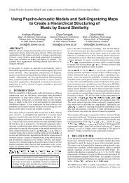
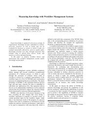
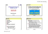

![Informationsvisualisierung [WS0708 | 01 ]](https://img.yumpu.com/22537403/1/190x143/informationsvisualisierung-ws0708-01-.jpg?quality=85)