Synthesis of Coupler Curves of Spherical Four-bar ... - IFToMM
Synthesis of Coupler Curves of Spherical Four-bar ... - IFToMM
Synthesis of Coupler Curves of Spherical Four-bar ... - IFToMM

You also want an ePaper? Increase the reach of your titles
YUMPU automatically turns print PDFs into web optimized ePapers that Google loves.
12th <strong>IFToMM</strong> World Congress, Besançon (France), June18-21, 2007<br />
<strong>Synthesis</strong> <strong>of</strong> <strong>Coupler</strong> <strong>Curves</strong> <strong>of</strong> <strong>Spherical</strong> <strong>Four</strong>-<strong>bar</strong> Mechanism<br />
Through Fast <strong>Four</strong>ier Transform<br />
Jinkui Chu * Jianwei Sun †<br />
Key Laboratory for Precision and Non-traditional Machining Technology <strong>of</strong> Ministry <strong>of</strong> Education;<br />
Key Laboratory for Micro/Nano Technology and System <strong>of</strong> Liao-ning Province<br />
DaLian 116023, P. R. China<br />
DaLian 116023, P. R. China<br />
Abstract—In this paper , the mathematic representation <strong>of</strong><br />
coupler curve <strong>of</strong> the spherical four-<strong>bar</strong> mechanisms is proposed.<br />
Base on the expression, the relationship between coupler curve<br />
and the basic dimensional types is discovered, and the formulas<br />
which can compute the position for coupler point, true size and<br />
installing dimensions <strong>of</strong> the spherical four-<strong>bar</strong> mechanism is<br />
deduced. These formulas make the spherical four-<strong>bar</strong> mechanism<br />
path generation with prescribed timing be possible. Finally, an<br />
example is given to prove it<br />
.<br />
Keywords: <strong>Spherical</strong> four-<strong>bar</strong> mechanism, Path generator,<br />
Harmonic component, Dimension synthesis<br />
mechanism, and use these formulas to approach the<br />
problems <strong>of</strong> path generation with prescribed timing.<br />
II. Mathematical description <strong>of</strong> basic geometric<br />
constructions<br />
I. Introduction<br />
Path generation problems in planar has been extensively<br />
studied. It seems that investigations specifically dealing<br />
with path generating problems in spherical kinematics are<br />
relatively few. In recent years, there is a tendency to use<br />
spherical mechanism; more and more authors used<br />
different means to solve this problem. Tong [1] discussed<br />
the syntheses <strong>of</strong> planar and spherical four-<strong>bar</strong> path<br />
generators by using the pole method. Chiang [2] presented<br />
a discussion <strong>of</strong> the spherical four-<strong>bar</strong> path generator to<br />
generate a coupler curve passing through four given path<br />
points. Moreover, Bagci [3] proposed an approach to treat<br />
path generating by means <strong>of</strong> geometric methods. The<br />
Symmetrical coupler curve and singular point<br />
classification in planar and spherical swinging-block<br />
linkages have been discussed in Shirazi [4].Chu [5] study<br />
the coupler curve <strong>of</strong> planar four-<strong>bar</strong> linkages in the<br />
frequency field by using the complex vector and frequency<br />
method. And base on the theory, the synthesis <strong>of</strong> coupler<br />
curves <strong>of</strong> planar four-<strong>bar</strong> linkages through fast <strong>Four</strong>ier<br />
transforms was investigated<br />
[6-8] . In this paper, by<br />
discussing the relationship between coupler curve <strong>of</strong> the<br />
spherical four-<strong>bar</strong> mechanism and it’s harmonic<br />
composition, we determine the basic dimensional type <strong>of</strong><br />
spherical four-<strong>bar</strong> mechanism and deduce the formulas<br />
which may compute the position for coupler point, true<br />
size and installing dimensions <strong>of</strong> the spherical four-<strong>bar</strong><br />
*E-mail: chujk@dlut.edu.cn<br />
† E-mail: avensun@tom.com<br />
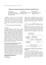
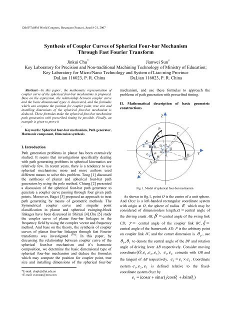
Fig. 1. Model <strong>of</strong> spherical four-<strong>bar</strong> mechanism<br />
As shown in fig.1, point O is the centre <strong>of</strong> a unit sphere.<br />
And Oxyz is a left-handed rectangular coordinate system<br />
with origin at O, the sphere <strong>of</strong> radius R which may be<br />
considered <strong>of</strong> dimensionless length, α = central angle <strong>of</strong><br />
the driving crank AB, β = central angle <strong>of</strong> the swing link<br />
CD, γ = central angle <strong>of</strong> the coupler link BC, ξ =<br />
central angle <strong>of</strong> the framework AD. P is the arbitrary point<br />
on coupler link BC, and the corner dimension is θ<br />
p<br />
, use<br />
θ ,θ 0 1<br />
to denote the central angle <strong>of</strong> the BP and rotation<br />
angle <strong>of</strong> driving lever AB respectively. Consider moving<br />
coordinate ( O, e1,<br />
e2<br />
, e ) , e ,e<br />
3 1 2<br />
coincide with OB and<br />
the tangent <strong>of</strong> AB respectively, e<br />
3<br />
= e1<br />
× e2<br />
. Coordinate<br />
system e1 , e2<br />
, e3<br />
is defined relative to the fixedcoordinate<br />
system Oxyz by<br />
e<br />
1<br />
= icosα<br />
+ sinα(<br />
jcosθ1<br />
+ ksinθ1)
12th <strong>IFToMM</strong> World Congress, Besançon (France), June18-21, 2007<br />
= i cosα<br />
+ jsinαcosθ1 + ksinαsinθ1<br />
(1)<br />
e<br />
2<br />
= jcos(<br />
θ<br />
1<br />
+ π / 2) + ksin(<br />
θ1<br />
+ π / 2)<br />
= − j sinθ1 + k cosθ1<br />
(2)<br />
e<br />
3<br />
= isinα<br />
− cosα<br />
( jcosθ1<br />
+ ksinθ1)<br />
= isinα<br />
− jcosαcosθ1 − kcosαsinθ1<br />
(3)<br />
Where: θ<br />
1<br />
= Q + ωt<br />
; Q is initial angle <strong>of</strong> the<br />
driving crank<br />
Positions <strong>of</strong> point P may be expressed in terms <strong>of</strong> the<br />
coordinate system Oe e as follows:<br />
1 2e3<br />
x<br />
pe<br />
= R cosθ 0<br />
(4)<br />
y<br />
pe<br />
= −R<br />
sinθ 0<br />
sin( θ<br />
2<br />
+ θ<br />
p<br />
) (5)<br />
z<br />
pe<br />
= R sin θ<br />
0<br />
cos( θ<br />
2<br />
+ θ<br />
p<br />
) (6)<br />
We obtain the positions <strong>of</strong> point P in terms <strong>of</strong> the<br />
fixed-coordinate system Oxyz as follows:<br />
r = x e + y e + z e<br />
Where ( e<br />
p pe 1 pe 2<br />
1<br />
, e2<br />
, e3<br />
, xpe<br />
, y<br />
pe<br />
, z<br />
pe<br />
pe<br />
3<br />
) was defined by<br />
Equation (1-6). Thus<br />
r = i cosθ cosα<br />
+ sinθ<br />
cos( θ + θ )sinα<br />
] R<br />
p<br />
[<br />
0<br />
0 2 p<br />
[ cosθ 0cosθ1sinα<br />
+ sinθ<br />
0sinθ1sin(<br />
θ<br />
2<br />
+ θ<br />
p<br />
− sinθ 0cos(<br />
θ<br />
2<br />
+ θ<br />
p<br />
)cosαcosθ1<br />
[ cosθ 0sinθ1sinα<br />
− sinθ<br />
0cosθ1sin(<br />
θ<br />
2<br />
+ θ<br />
p<br />
− sinθ 0cos(<br />
θ<br />
2<br />
+ θ<br />
p<br />
)cosαsinθ1<br />
+ j<br />
+ k<br />
The y axis and z axis are defined as the real axis and<br />
imaginary axis respectively. Above equation reduces to<br />
r = i cosθ cosα<br />
+ sinθ<br />
cos( θ + θ )sinα<br />
] R<br />
p<br />
[<br />
0<br />
0 2 p<br />
+ R [ cosθ<br />
0<br />
sinα<br />
− sinθ<br />
0<br />
(cos( θ<br />
2<br />
+ θ<br />
p<br />
)<br />
]R<br />
)<br />
]R<br />
) cosα<br />
+ k sin(<br />
θ + θ ))]e<br />
Where k = −1<br />
When the mechanism lies in standard installing position,<br />
and the angular velocity <strong>of</strong> input link AB is constant<br />
parameter ω (the input angle θ 1<br />
can be expressed as<br />
θ<br />
1<br />
= ωt ), the rpx<br />
which is the projection <strong>of</strong> rp<br />
on the x<br />
axis may be expressed as follow:<br />
r t)<br />
= Rcosθ cosα<br />
px<br />
(<br />
0<br />
t =<br />
2<br />
p<br />
kθ<br />
+ R sinθ<br />
cos( θ ( t)<br />
θ ) sinα<br />
(7)<br />
θ /<br />
1<br />
ω<br />
0 2<br />
+<br />
Where:<br />
The standard installing position means that the angle<br />
Q between AB and CD is 0°<br />
(defined the angle Q is<br />
initial angle <strong>of</strong> the driving crank); the frame AD lies on x-y<br />
plane; the centre <strong>of</strong> sphere is located at the origin <strong>of</strong><br />
coordinate.<br />
p<br />
1<br />
Similarly for the projection <strong>of</strong> on the y-z plane we<br />
have<br />
r t)<br />
= R[cosθ<br />
sinα<br />
− sinθ<br />
(cos( θ ( t)<br />
θ ) cosα<br />
pyz<br />
(<br />
0<br />
0 2<br />
+<br />
p<br />
kθ1<br />
+ k sin(<br />
θ<br />
2<br />
( t)<br />
+ θ<br />
p<br />
))]e (8)<br />
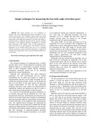
Figure.2 is a spherical four-<strong>bar</strong> mechanism (mechanism<br />
lies in general installing position), where O<br />
x<br />
, O<br />
y<br />
, Oz<br />
is<br />
the distance between O and O'<br />
, θ<br />
x<br />
is defined as the<br />
angle between the y' axis and the y axis measured in<br />
accord with the right-hand convention from y axis and the<br />
y ' axis about the x'<br />
axis.<br />
Fig. 2. General position <strong>of</strong> spherical four-<strong>bar</strong> mechanism<br />
In this case, base on the Equation (7),<br />
r p<br />
r p<br />
which is the<br />
projection <strong>of</strong> on the x axis, can be expressed as follow:<br />
rpx<br />
( t + t′<br />
) = Ox + Rcosθ 0cosα<br />
+ R sinθ<br />
0<br />
cos( θ<br />
2<br />
( t + t′<br />
) + θ<br />
p<br />
) sinα<br />
(9)<br />
Where: t ' = Q / ω<br />
Similarly, base on the Equation (8), for the projection <strong>of</strong><br />
r p<br />
on the y-z plane we have<br />
r<br />
r px<br />
kμ<br />
kθ<br />
x<br />
t + t′<br />
) = R' e + e R[cosθ<br />
sinα<br />
- sinθ<br />
0<br />
(cos( θ<br />
2<br />
( t + t′ ) + θ<br />
p<br />
) cosα<br />
kθ1<br />
+ k sin(<br />
θ ( t + t′<br />
) + θ ))]e<br />
pyz<br />
(<br />
0<br />
Where<br />
R'<br />
2<br />
y<br />
2<br />
z<br />
= O + O and<br />
2<br />
p<br />
μ = arctan<br />
O<br />
O<br />
z<br />
y<br />
(10)<br />
Equations (9), (10) will be used to discuss the<br />
relationship between coupler curve <strong>of</strong> the spherical<br />
four-<strong>bar</strong> mechanism and its harmonic composition
12th <strong>IFToMM</strong> World Congress, Besançon (France), June18-21, 2007<br />
III. Frequency analysis <strong>of</strong> the spherical four-<strong>bar</strong><br />
mechanism’s coupler curve.<br />
The θ<br />
2<br />
( t)<br />
+ θ<br />
p<br />
is a periodic function whose<br />
periodicity is 2 π , so Equation (9) is also a periodic<br />
function, and it’s periodicity was determined by the<br />
function <strong>of</strong> cos(<br />
θ<br />
2<br />
( t + t′ ) + θ<br />
p<br />
) .Defined the one<br />
dimensional <strong>Four</strong>ier expansion <strong>of</strong> cos(<br />
θ<br />
2<br />
( t ) + θ<br />
p<br />
) can<br />
be expressed as follow:<br />
∑ ∞ kϕ<br />
knω<br />
2<br />
( t)<br />
+ θ<br />
p<br />
) = c<br />
ne<br />
e<br />
n=<br />
−∞<br />
n t<br />
cos(<br />
θ (11)<br />
c<br />
Where<br />
n<br />
and ϕ<br />
n<br />
are the <strong>Four</strong>ier series’ amplitude<br />
and phase angle respectively.<br />
Substituting Equation (11) in Equation (9) yields<br />
r t + t′<br />
) = Ox + Rcosθ cosα<br />
px<br />
(<br />
0<br />
+ Rsin<br />
θ sinα<br />
0<br />
∑ ∞ n<br />
n=<br />
−∞<br />
c e<br />
k(<br />
ϕ + nQ)<br />
Merge the 0 item <strong>of</strong> the <strong>Four</strong>ier series, we can obtain<br />
r px<br />
( t + t′<br />
)<br />
kϕ0<br />
= ( O + Rcosθ<br />
cosα<br />
+ Rc<br />
sinθ<br />
sinαe<br />
)<br />
x<br />
0<br />
0<br />
∑<br />
0<br />
n<br />
e<br />
knωt<br />
k ( ϕ n + nQ) knωt<br />
+ sinθ0sinα<br />
cne<br />
e<br />
n ≠0<br />
kϕ −1<br />
c−<br />
1<br />
e , we have<br />
1 −kϕ<br />
∑ ∞ c<br />
− 1 n k ( ϕn<br />
−ϕ−<br />
) n t<br />
cos(<br />
2<br />
( ) +<br />
p<br />
)e = e<br />
1 k ω<br />
θ t θ<br />
e<br />
−1<br />
n=<br />
−∞ c<br />
−1<br />
Equation (11) dividing by<br />
c<br />
R (12)<br />
Equation (12) dividing by Rc<br />
−1sinθ<br />
0sinαe<br />
have<br />
r ( + ′<br />
px<br />
t t )<br />
k ( Q− −1<br />
)<br />
e<br />
ϕ =<br />
R c<br />
-1sinθ<br />
0sinα<br />
1<br />
(O<br />
x<br />
+ Rcosθ<br />
0cosα<br />
R c<br />
-1sinθ<br />
0sinα<br />
kϕ0 −k<br />
( ϕ −<br />
+ Rc<br />
sinθ<br />
sinαe<br />
) e<br />
0<br />
+<br />
0<br />
∑<br />
k ( ϕ − 1 −Q)<br />
1<br />
−Q)<br />
(13)<br />
, we<br />
c n k ( ϕ n −ϕ<br />
− 1 + (n + 1)Q) knωt<br />
(14)<br />
n ≠0<br />
c−<br />
1<br />
By comparing the equation (13) with the equation (14),<br />
we can find that they have the same amplitude (except the<br />
0 item) and the equation (13)’s phase angle subtracted<br />
from equation (14)’s phase angle gives ( n + 1)Q .<br />
Theθ 2<br />
( t)<br />
+ θ<br />
p<br />
is a periodic function whose periodicity<br />
is 2 π , so Equation (10) is also a periodic function, and the<br />
periodicity was determined by the function <strong>of</strong><br />
cos(<br />
θ ( t ) + θ )cosα<br />
+ ksin(<br />
θ ( t)<br />
+ ) .Defined<br />
2 p<br />
2<br />
θ<br />
p<br />
e<br />
e<br />
the two-dimensional <strong>Four</strong>ier expansion <strong>of</strong> the expression<br />
can be expressed as follow:<br />
cos(<br />
θ ( t ) + θ )cosα<br />
+ ksin(<br />
θ ( t)<br />
+ )<br />
=<br />
∑ ∞ n<br />
n = −∞<br />
c'<br />
2 p<br />
2<br />
θ<br />
p<br />
n ω<br />
c' e e<br />
k ϕ ' kn<br />
t<br />
(15)<br />
Where<br />
n<br />
and ϕ'<br />
n<br />
are the <strong>Four</strong>ier series’ amplitude and<br />
phase angle respectively.<br />
Substituting Equation (15) in Equation (10) yields<br />
r<br />
′<br />
kμ<br />
kθ<br />
x<br />
pyz<br />
( t + t ) = R' e + e<br />
0<br />
R[cosθ<br />
sinα<br />
− sinθ<br />
(<br />
0 ∑ ∞ c'<br />
n<br />
n = -∞<br />
e<br />
k ( ϕ ' n + nQ)<br />
e<br />
knωt<br />
Merge the 1 item <strong>of</strong> the <strong>Four</strong>ier series, we can obtain<br />
r<br />
( t + t′<br />
) = R' e<br />
kμ<br />
pyz<br />
kϕ<br />
' 0 k ( θx<br />
+ Q) kωt<br />
R( cosθ<br />
0sinα<br />
− c'<br />
0<br />
sinθ<br />
0e<br />
)e e<br />
+<br />
− R sinθ<br />
∑<br />
)] e<br />
k ( ϕ'<br />
n + (n+<br />
1)Q+<br />
θ x ) k (n+<br />
1) ωt<br />
0<br />
c'<br />
n<br />
e e<br />
n≠0<br />
Merge the 0 item <strong>of</strong> the <strong>Four</strong>ier series and defined<br />
n = n + 1, we have<br />
r<br />
pyz<br />
( t + t′<br />
) = (R' e<br />
+ R<br />
− Rc'<br />
sinθ<br />
e<br />
kμ<br />
k ( ϕ'<br />
-1 + θ x )<br />
−1<br />
0<br />
kϕ<br />
' 0 k ( θx<br />
+ Q) kωt<br />
( cosθ<br />
0sinα<br />
− c'<br />
0<br />
sinθ<br />
0e<br />
)e e<br />
∑<br />
k ( ϕ ' n -1 + nQ+<br />
θ x ) knωt<br />
0<br />
c'<br />
n-1<br />
e e<br />
n≠0,1<br />
kϕ − 2<br />
e<br />
′<br />
−<br />
, we have<br />
)<br />
kθ1<br />
− R sinθ<br />
(16)<br />
Equation (15) dividing by c'<br />
2<br />
1 -kϕ′<br />
e<br />
- 2<br />
(cos( θ<br />
2<br />
( t)<br />
+ θ<br />
p<br />
)cosα<br />
+ ksin(<br />
θ<br />
2<br />
( t)<br />
+<br />
p<br />
)) =<br />
c′<br />
θ<br />
-2<br />
∑ ∞ c' n k ( ϕ ' n −ϕ<br />
' − ) n t<br />
e<br />
2 k ω<br />
e<br />
(17)<br />
n=<br />
−∞ c'<br />
−2<br />
k ( ϕ′<br />
2 −2Q)<br />
Equation (16) dividing by Rc−2sinθ0e<br />
−<br />
, we can<br />
obtain<br />
r ( + ′<br />
pyz<br />
t t )<br />
k (2 Q − − ′ 2<br />
e<br />
ϕ ) 1<br />
kμ<br />
= - [(R' e<br />
R c′<br />
-2sinθ<br />
0<br />
Rc'<br />
-2<br />
sinθ<br />
0<br />
k ( ϕ '-1 + θx<br />
) -k<br />
( ϕ '-2<br />
-Q+<br />
θx<br />
)<br />
− R c' sinθ<br />
e )]e<br />
−<br />
c'<br />
−1<br />
0<br />
1 kϕ<br />
' 0 k (2Q-ϕ<br />
'-2<br />
) kωt<br />
[(cosθ<br />
0sinα<br />
− c'<br />
0<br />
sinθ<br />
0e<br />
)]e e<br />
−2<br />
sinθ<br />
0<br />
∑<br />
c' 2<br />
n −1<br />
k ( ϕ ' n −1<br />
−ϕ<br />
' − + (n + 1)Q) knωt<br />
+ e<br />
e (18)<br />
n ≠0,1<br />
c'<br />
−2<br />
By comparing the equation (17) with the equation (18),<br />
we can find that they have the same amplitude (except the<br />
0 item and the 1 item) and the equation (17)’s phase angle<br />
subtracted from equation (18)’s phase angle gives<br />
( n + 1) Q + ϕ'<br />
n − 1-ϕ<br />
'<br />
n<br />
.
12th <strong>IFToMM</strong> World Congress, Besançon (France), June18-21, 2007<br />
These findings indicate that the <strong>Four</strong>ier series <strong>of</strong> the<br />
general position <strong>of</strong> spherical four-<strong>bar</strong> mechanism’s coupler<br />
curve mostly depend on equation (13) and equation (17),<br />
and the equations were determined by mechanism’s basic<br />
dimensional types which includeα , γ , β , ξ and θ p<br />
. We<br />
can calculate coupler rotation-angle θ<br />
2<br />
<strong>of</strong> the mechanism<br />
basic dimensional type, and obtain corresponding<br />
harmonic component’s database by utilizing one<br />
dimension and two dimensions FFT. Finally, constitute a<br />
numerical atlas database by put the harmonic component’s<br />
database and mechanisms’ basic dimensional types<br />
together. By comparing the harmonic characteristic<br />
components <strong>of</strong> the given coupler curve with the harmonic<br />
characteristic component <strong>of</strong> every group in the numerical<br />
atlas and utilizing fuzzy identification in Ref.[10], the<br />
weighting hamming distance can be figured out.<br />
According to fuzzy theory, weighting hamming distance<br />
can measure the similarity degree <strong>of</strong> the referred model<br />
and identified object. The two parts will more approximate<br />
when the distance is smaller. If the distance is equal to<br />
zero, the two are the same. The basic dimensional types <strong>of</strong><br />
linkage are determined by this method.<br />
IV. Compute the position for coupler point, true size<br />
and installing dimensions <strong>of</strong> the spherical four-<strong>bar</strong><br />
mechanism<br />
Defined<br />
r<br />
px<br />
kζ knωt<br />
∑ ∞ n<br />
ne<br />
e<br />
n = −∞D<br />
= is the harmonic<br />
component <strong>of</strong> the given coupler curve<br />
and<br />
r<br />
pyz<br />
kζ ' knωt<br />
∑ ∞ n<br />
'<br />
n<br />
e e<br />
n=<br />
−∞D<br />
r p<br />
project on x axis,<br />
= is the harmonic<br />
component <strong>of</strong> the given coupler curve<br />
plane.<br />
(1)Central angle <strong>of</strong> the driving crank α<br />
From equations (12) (16), we know that<br />
D'<br />
r p<br />
project on y-z<br />
n<br />
R sinθ<br />
0<br />
= (n ≠ 0,1) (19)<br />
c'<br />
n−1<br />
D<br />
sin sin =<br />
n<br />
R θ<br />
0<br />
α (n ≠ 0,1) (20)<br />
c<br />
n<br />
Substituting Equation (19) into Equation (20) yields<br />
D<br />
nc'<br />
n<br />
= arcsin(<br />
D' c<br />
)<br />
−1<br />
α (n ≠ 0,1) (21)<br />
n n<br />
The other basic dimensional types can be obtained by<br />
the proportional relation.<br />
(2) Initial angle <strong>of</strong> the driving crank Q<br />
From equations (11) (12), we can obtain<br />
Q = ζ −<br />
(22)<br />
1<br />
ϕ 1<br />
(3) Turn angle θ<br />
x<br />
From equations (15) (16), we know that<br />
ζ ' = −Q + θ<br />
(23)<br />
- 1<br />
ϕ'<br />
-2<br />
From equation (23) we can obtain<br />
x<br />
-1<br />
x<br />
θ = ζ ' + Q − ϕ'<br />
(24)<br />
(4) The sphere <strong>of</strong> radius R<br />
From equation (16), we know that<br />
kζ<br />
' 1 kϕ'<br />
0 k(<br />
θx<br />
+ Q)<br />
D' 1<br />
e = R(cosθ 0<br />
sinα<br />
− sinθ0c'<br />
0<br />
e ) e (25)<br />
From equation (25) we can obtain<br />
2<br />
2 2<br />
R = A + ( D n<br />
/ c ) ) / sin α (26)<br />
Where<br />
D<br />
(<br />
n<br />
A = [ D'<br />
1<br />
cosζ<br />
'<br />
1−<br />
'<br />
n<br />
c'<br />
0<br />
cos( ϕ '<br />
0<br />
+ θ<br />
x<br />
+ Q)<br />
/ c'<br />
n−1<br />
]/ cos( θ<br />
x<br />
+ Q<br />
θ<br />
(5) Central angle<br />
0<br />
From equation (19), we can obtain<br />
-2<br />
D'<br />
= arcsin(<br />
Rc'<br />
n<br />
θ<br />
0<br />
(27)<br />
n−1<br />
(6) Translational component on x axis Ox<br />
From equation (12), we know that<br />
D0 cosζ<br />
0<br />
= O x<br />
+ cosθ<br />
0sinα<br />
+ c0sinθ0sinαcosϕ0<br />
(28)<br />
From equation (28), we can obtain<br />
O<br />
x<br />
= D0cosζ<br />
0<br />
− cosθ<br />
0sinα<br />
− c0sinθ0sinαcosϕ0<br />
(29)<br />
(7) Translational component on y axis and z axis O<br />
y<br />
, Oz<br />
From equation (16), we know that<br />
kζ<br />
' 0 kμ<br />
k ( ϕ '-1<br />
+ θ x )<br />
D'<br />
0<br />
e = R' e − c'<br />
−1<br />
sinθ<br />
0e<br />
(30)<br />
From equation (30), we can obtain<br />
O<br />
y<br />
= D'<br />
0<br />
cosζ '<br />
0<br />
+ c'<br />
−1<br />
sinθ<br />
0cos(<br />
ϕ'<br />
−1<br />
+ θ<br />
x<br />
) (31)<br />
O<br />
z<br />
= D'<br />
0<br />
sinζ '<br />
0<br />
+ c'<br />
−1<br />
sinθ<br />
0sin(<br />
ϕ'<br />
−1<br />
+ θ<br />
x<br />
) (32)<br />
Base on the equations (21)(22)(24)(26)(27)(29)(31)(32),<br />
we can compute the position for coupler point, true size<br />
and installing dimensions <strong>of</strong> the spherical four-<strong>bar</strong><br />
mechanism.<br />
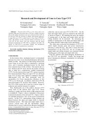
V. Illustration<br />
Figure 3 shows the given coupler curve, (a) the given<br />
coupler curve; (b) the coupler curve project on x-y plane;<br />
(c) the coupler curve project on x-z plane; (d) the coupler<br />
curve project on y-z plane. Suppose a spherical four-<strong>bar</strong><br />
linkages is to be synthesized to generate the given coupler<br />
curve<br />
<strong>Spherical</strong> four-<strong>bar</strong> mechanism path generation will be<br />
done by using the follow steps. First, based on those<br />
sampling points (in this paper, we choose 64 points and<br />
the sampling points are denoted by “+”), the<br />
)<br />
)
12th <strong>IFToMM</strong> World Congress, Besançon (France), June18-21, 2007<br />
corresponding harmonic component <strong>of</strong> the given couple<br />
curve can be obtained by utilizing one dimension and two<br />
dimension FFT. Second, carry out identification between<br />
the harmonic characteristic component got from first step<br />
and the corresponding component in the numerical atlas.<br />
Decide the basic dimensional types <strong>of</strong> mechanism by using<br />
fuzzy identification method. Finally, the true size and<br />
installing dimensions <strong>of</strong> the spherical four-<strong>bar</strong> mechanism<br />
can be computed by the basic dimensional types and the<br />
equations (21) (22) (24) (26) (27) (29) (31) and (32).The<br />
results are:<br />
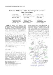
α = 23.0795° γ = 47.1624°<br />
β = 53.1831° ξ = 57.1969°<br />
θ = 68.0000° θ = 29.7188°<br />
p<br />
0<br />
θ = 15.5601° Q = 30.0578°<br />
x<br />
O = 9.9804mm O = -4.9766mm<br />
x<br />
y<br />
O = -5.9621mm R = 2.7231mm<br />
z<br />
Fig. 3. Given coupler curve <strong>of</strong> spherical four-<strong>bar</strong> mechanism<br />
Figure 4 shows the fitting comparison between the<br />
given coupler curve and the actual mechanisms’ coupler<br />
curve. The given coupler is denoted by “—” and the actual<br />
mechanisms’ coupler curve is denoted by “·”.<br />
VI. Conclusion<br />
The spherical four-<strong>bar</strong> mechanism is the most basic and<br />
useful spherical hinge which can be used to many<br />
machines. Because the spherical mechanism have more<br />
parameters, the path generation is harder than plane<br />
mechanism’s. The usual method used for path generation<br />
only solve the finitely separated path-points or a segment<br />
<strong>of</strong> coupler curve, the method we have proposed makes the<br />
closed coupler curve generation be possible.<br />
VII. Acknowledgements<br />
This project was supported by the National Natural<br />
Science Foundation <strong>of</strong> China (Grant No. 50475153) and<br />
the Foundation <strong>of</strong> Ministry <strong>of</strong> Education (NCET-04-0266)<br />
Reference<br />
[1] Shih-his Tong and C.H.Chiang. Syntheses <strong>of</strong> Planar and <strong>Spherical</strong><br />
<strong>Four</strong>-Bar Path Generators By the Pole Method. Mechanism and<br />
Machine Theory, 27(2):143–155, 1992.<br />
[2] Cemil Bagci. Geometric Methods for the <strong>Synthesis</strong> <strong>of</strong> <strong>Spherical</strong><br />
Mechanisms for the Generation <strong>of</strong> Functions, Paths and Rigid-Body<br />
Positions Using Conformal projections. Mechanism and Machine<br />
Theory, 19(2):113–127, 1984.<br />
[3] C.H.Chiang. Syntheses <strong>of</strong> <strong>Spherical</strong> <strong>Four</strong>-Bar Path Generators.<br />
Mechanism and Machine Theory, 21:135–143, 1986.<br />
[4] Shirazi and Kourosh h. Symmetrical <strong>Coupler</strong> Curve and Singular<br />
Point Classification in Planar and <strong>Spherical</strong> Swinging-Block<br />
Linkages. Journal <strong>of</strong> Mechanical Design Transactions <strong>of</strong> the ASME,<br />
128(2):436-443, March 2006.<br />
[5] Chu jinkui and others. Frequency Analysis <strong>of</strong> the planar Linkage's<br />
<strong>Coupler</strong> <strong>Curves</strong>. Jixie Kexue Yu Jishu/Mechanical Science and<br />
Technology, 41(1):1-5, January 1992.<br />
[6] Chu jinkui and Cao weiqing. <strong>Synthesis</strong> <strong>of</strong> <strong>Coupler</strong> <strong>Curves</strong> <strong>of</strong> Planar<br />
<strong>Four</strong>-Bar Linkages Through Fast <strong>Four</strong>ier Transform. Chinese journal<br />
<strong>of</strong> mechanism engineer, 29(5):117-122, October 1993.<br />
[7] Chu jinkui and others. Relationship between properties <strong>of</strong> coupler<br />
curve and link's dimensions in 4-<strong>bar</strong> mechanisms and its' application.<br />
Proceeding <strong>of</strong> the 2004 the Eleventh World Congress in Mechanism<br />
and Machine Science, Proceedings <strong>of</strong> the 2004 - the Eleventh World<br />
Congress in Mechanism and Machine Science, 1274-1279, 2004<br />
[8] Wu xin and others. Dimensional <strong>Synthesis</strong> for Planar 4-Bar Path<br />
Generator with Prescribed Timing. Jixie Kexue Yu Jishu/Mechanical<br />
Science and Technology, 17(6):885-888, November 1998.<br />
[9] John. R. McGarya. Rapid search and selection <strong>of</strong> path generating<br />
mechanisms from a library. Mechanism and Machine Theory,<br />
29(2):223–235, 1994<br />
[10] Huo jngping and Cao weiqing. Fuzzy mathematics method for locus<br />
synthesis <strong>of</strong> planer four-<strong>bar</strong> linkage. Chinese journal <strong>of</strong> mechanism<br />
engineer. 3 (1) : 23-28,1990<br />
[11] G N. Sandor. and A G.Erdman. Advanced Mechanism Design:<br />
Analysis and <strong>Synthesis</strong>, Vol.2, 1984,<br />
Fig. 4. Fitting comparison between the given coupler curve and theactual<br />
coupler curve <strong>of</strong> spherical four-<strong>bar</strong> mechanism