ENTRY CURVES - Harvard University
ENTRY CURVES - Harvard University
ENTRY CURVES - Harvard University
Create successful ePaper yourself
Turn your PDF publications into a flip-book with our unique Google optimized e-Paper software.
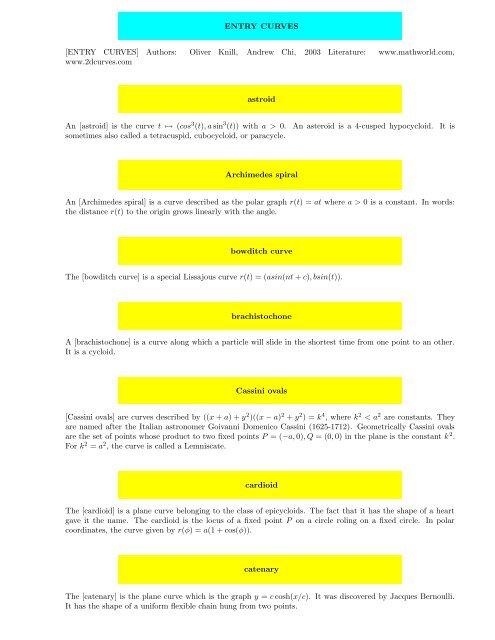
<strong>ENTRY</strong> <strong>CURVES</strong><br />
[<strong>ENTRY</strong> <strong>CURVES</strong>] Authors: Oliver Knill, Andrew Chi, 2003 Literature: www.mathworld.com,<br />
www.2dcurves.com<br />
astroid<br />
An [astroid] is the curve t ↦→ (cos 3 (t), a sin 3 (t)) with a > 0. An asteroid is a 4-cusped hypocycloid. It is<br />
sometimes also called a tetracuspid, cubocycloid, or paracycle.<br />
Archimedes spiral<br />
An [Archimedes spiral] is a curve described as the polar graph r(t) = at where a > 0 is a constant. In words:<br />
the distance r(t) to the origin grows linearly with the angle.<br />
bowditch curve<br />
The [bowditch curve] is a special Lissajous curve r(t) = (asin(nt + c), bsin(t)).<br />
brachistochone<br />
A [brachistochone] is a curve along which a particle will slide in the shortest time from one point to an other.<br />
It is a cycloid.<br />
Cassini ovals<br />
[Cassini ovals] are curves described by ((x + a) + y 2 )((x − a) 2 + y 2 ) = k 4 , where k 2 < a 2 are constants. They<br />
are named after the Italian astronomer Goivanni Domenico Cassini (1625-1712). Geometrically Cassini ovals<br />
are the set of points whose product to two fixed points P = (−a, 0), Q = (0, 0) in the plane is the constant k 2 .<br />
For k 2 = a 2 , the curve is called a Lemniscate.<br />
cardioid<br />
The [cardioid] is a plane curve belonging to the class of epicycloids. The fact that it has the shape of a heart<br />
gave it the name. The cardioid is the locus of a fixed point P on a circle roling on a fixed circle. In polar<br />
coordinates, the curve given by r(φ) = a(1 + cos(φ)).<br />
catenary<br />
The [catenary] is the plane curve which is the graph y = c cosh(x/c). It was discovered by Jacques Bernoulli.<br />
It has the shape of a uniform flexible chain hung from two points.
catenoid<br />
The [catenoid] is the surface obatained by rotating the catenary about the x-axis. The minimal surface bounded<br />
by two coaxial rings can be a catenoid.<br />
circle<br />
A [circle] in the plane is the curve r(t) = (r cos(t), r sin(t)) where the radius r is a constant. It is the set of<br />
points which have a fixed distance r from the origin. More generally, a circle is the set of points in a metric<br />
space which have a fixed distance from a given point.<br />
cissoid<br />
A [cissoid] is a plane curve given in Euclidean coordinates by y 2 (2a − x) = x 3 . In polar coordinates, it satisfies<br />
r(t) = 2a tan(t) sin(t) or in Euclidean coordinates r(t) = (2a sin 2 (t), 2a sin 3 (t)/ cos(t)). The curve has a cusp at<br />
the origin. It was first mentioned by Diocles in 180 B.C.<br />
conic section<br />
A [conic section] is a nondegenerate curve generated by intersecting a plane with one or two nappes of a cone.<br />
The three congruence classes of conic sections are the ellipse, the parabola, and the hyperbola.<br />
ellipse<br />
An [ellipse] is the locus of all points in the plane the sum of whose distances from two fixed points is a positive<br />
constant. It is also the conic section which results from a plane which intersects only one nappe of the cone.<br />
The general formula for an ellipse up to rotation and translation is x2<br />
a<br />
+ y2<br />
2 b<br />
= 1.<br />
2<br />
hyperbola<br />
A [hyperbola] is the set of points in the plane for which the difference of the distances from two fixed points is<br />
a constant. It is also the conic section which results from a plane intersecting a cone. The general formula for<br />
a hyperbola up to rotation and translation is x2<br />
a<br />
− y2<br />
2 b<br />
= 1.<br />
2<br />
curve<br />
A [curve] is a continuous map from the real line to an the plane or to space. The word ”curve” is often used to<br />
mean the image of this map. Curves can be represented parametrically by r(t) = (x(t), y(t)) or implicitely as<br />
f(x, y) = 0.
Airy function<br />
The [Airy function] is commonly found as a solution to boundary value problems in quantum mechanics and<br />
electromagnetism. It is the solution to the differential equation: y ′′ = xy. The two independent solutions are<br />
(without constants):<br />
∫ ∞<br />
( ) t<br />
3<br />
Ai(x) = cos<br />
0 3 + xt dt<br />
∫ ∞<br />
(<br />
( ))<br />
Bi(x) = e − t3 t<br />
3 +xt 3<br />
+ sin<br />
3 + xt dt<br />
0<br />
algebraic curve<br />
A plane curve is an [algebraic curve] if it is given by g(x, y) = 0 where g is algebraic a polynomial in x and y.<br />
An algebraic curve with degree greater than 2 is called a higher plane curve. The circle g(x, y) = x 2 +y 2 −1 = 0<br />
is an example of an algebraic curve, the catenary g(x, y) = y − c cosh(x/c) = 0 is an example of a nonalgebraic<br />
curve.<br />
cubic curve<br />
A [cubic curve] is an algebraic curve of order three. Newton showed that all cubics can be generated as<br />
projections of the five divergent cubic parabolas. Examples include the cissoid of Diocles and ellptic curves.<br />
ampersand curve<br />
The [ampersand curve] is a quartic curve with implicit equation (y 2 − x 2 )(x − 1)(2x − 3) = 4(x 2 + y 2 − 2x) 2 .<br />
It looks like an ampersand.<br />
bean curve<br />
The [bean curve] is a quartic curve given by the implicit equation: x 4 + x 2 y 2 + y 4 = x(x 2 + y 2 ). It looks like a<br />
bean.<br />
bicorn<br />
The [bicorn] is the name of a collection of quartic curves studied by Sylvester in 1864 and Cayley in 1867. It is<br />
given by y 2 (a 2 − x 2 ) = (x 2 + 2ay − a 2 ) 2 .<br />
bicuspid<br />
The [bicuspid] is the quartic curve given by the implicit equation: (x 2 − a 2 )(x − a) 2 + (y 2 − a 2 ) 2 = 0.
ow<br />
The [bow] is a quartic curve with the implicit equation: x 4 = x 2 y − y 3 .<br />
cartesian oval<br />
A [cartesian oval] is a quartic curve consisting of two ovals. It is the locus of a point P whose distances from<br />
two foci F 1 and F 2 in two-center bipolar coordinates satisfy<br />
mr ± nr ′ = k<br />
where m and n are positive integers, k is a positive real, and r and r ′ are the distances from F 1 and F 2 . If<br />
m = n, then the oval becomes an ellipse.<br />
Cassini oval<br />
A [Cassini oval] is one of a family of quartic curves, also called Cassini ellipses, described by a point such that<br />
the product of its distances from two fixed points a distance 2a apart is constant b 2 . The shape of the curve<br />
depends on b/a. The Cassini ovals are defined in two-center bipolar coordinates by the equation r 1 r 2 = b 2<br />
where b is a positive constant.<br />
cruciform<br />
A [cruciform] is a plane quartic curve also called the cross curve or policeman on point duty curve. It is given<br />
by the implicit equation: x 2 y 2 − b 2 x 2 − a 2 y 2 = 0.<br />
lemniscate<br />
The [lemniscate], also known as the lemniscate of Bernoulli, is a polar curve whose most common form is the<br />
locus of points the product of whose distances from two fixed points a distance 2a away is the constant a 2 . The<br />
usual polar coordinate form is as follows: r 2 = a 2 cos(2θ).<br />
natural equation<br />
A [natural equation] is an equation which specifies a curve independent of any choice of coordinates or<br />
parametrization. This arose in the solution to the following problem: given two functions of one parameter,<br />
find the space curve for which the functions are the curvature and torsion. Often, the natural equation will<br />
be in terms of integrals.<br />
polynomial curve<br />
A [polynomial curve] is a curve obtained by fitting polynomials to a sequence of points. To fit curves better,<br />
splines like Bezier curve are more suited.
quadrifolium<br />
A [quadrifolium] is a rose curve with n = 2. It has polar equation<br />
r = a sin(2θ).<br />
sextic curve<br />
A [sextic curve] is an algebraic curve of degree 6. Examples include the atriphtaloid and the butterfly curve<br />
y 6 = x 2 − x 6 .<br />
atriphtaloid<br />
The [atriphtaloid] is a sextic curve also known as atriphtothlassic curve and given by the equation: x 4 (x 2 +<br />
y 2 ) − (ax 2 − b) 2 = 0.<br />
butterfly curve<br />
The [butterfly curve] is a sextic plane curve given by the implicit equation y 6 = x 2 − x 6 .<br />
trifolium<br />
A [trifolium] is the 3-petalled rose given in polar form as r(t) = a| cos(3t)|.<br />
spiral<br />
A [spiral], in general, is a curve with τ(s)/κ(s) constant for<br />
This file is part of the Sofia project sponsored by the Provost’s fund for teaching and learning at <strong>Harvard</strong><br />
university. There are 34 entries in this file.
Index<br />
Airy function, 3<br />
algebraic curve, 3<br />
ampersand curve, 3<br />
Archimedes spiral, 1<br />
astroid, 1<br />
atriphtaloid, 5<br />
bean curve, 3<br />
bicorn, 3<br />
bicuspid, 3<br />
bow, 4<br />
bowditch curve, 1<br />
brachistochone, 1<br />
butterfly curve, 5<br />
cardioid, 1<br />
cartesian oval, 4<br />
Cassini oval, 4<br />
Cassini ovals, 1<br />
catenary, 1<br />
catenoid, 2<br />
circle, 2<br />
cissoid, 2<br />
conic section, 2<br />
cruciform, 4<br />
cubic curve, 3<br />
curve, 2<br />
ellipse, 2<br />
hyperbola, 2<br />
lemniscate, 4<br />
natural equation, 4<br />
polynomial curve, 4<br />
quadrifolium, 5<br />
sextic curve, 5<br />
spiral, 5<br />
trifolium, 5<br />
6


