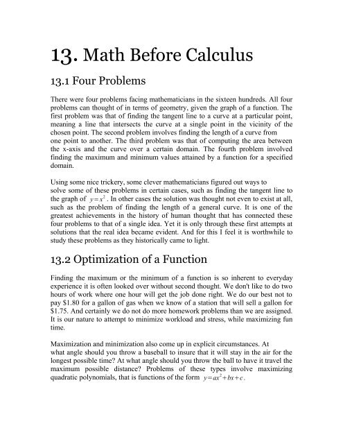
13.Math Before Calculus

13. Math Before Calculus
13.1 Four Problems
There were four problems facing mathematicians in the sixteen hundreds. All four
problems can thought of in terms of geometry, given the graph of a function. The
first problem was that of finding the tangent line to a curve at a particular point,
meaning a line that intersects the curve at a single point in the vicinity of the
chosen point. The second problem involves finding the length of a curve from
one point to another. The third problem was that of computing the area between
the x-axis and the curve over a certain domain. The fourth problem involved
finding the maximum and minimum values attained by a function for a specified
domain.
Using some nice trickery, some clever mathematicians figured out ways to
solve some of these problems in certain cases, such as finding the tangent line to
the graph of y=x 2 . In other cases the solution was thought not even to exist at all,
such as the problem of finding the length of a general curve. It is one of the
greatest achievements in the history of human thought that has connected these
four problems to that of a single idea. Yet it is only through these first attempts at
solutions that the real idea became evident. And for this I feel it is worthwhile to
study these problems as they historically came to light.
13.2 Optimization of a Function
Finding the maximum or the minimum of a function is so inherent to everyday
experience it is often looked over without second thought. We don't like to do two
hours of work where one hour will get the job done right. We do our best not to
pay $1.80 for a gallon of gas when we know of a station that will sell a gallon for
$1.75. And certainly we do not do more homework problems than we are assigned.
It is our nature to attempt to minimize workload and stress, while maximizing fun
time.
Maximization and minimization also come up in explicit circumstances. At
what angle should you throw a baseball to insure that it will stay in the air for the
longest possible time? At what angle should you throw the ball to have it travel the
maximum possible distance? Problems of these types involve maximizing
quadratic polynomials, that is functions of the form y=ax 2 bxc.

Example 13.2.1. Galileo found that if you throw a ball from the ground straight
upinto the air with the intial velocity (speed) of v 0 feet per second, then the height
in feet is given by
ht =−16 t 2 v 0
t .
Suppose we throw a ball straight up from the ground with initial velocity of 4 feet
per second. What is the maximum height the ball will reach? We can solve this
problem as before by expressing h as a translation of the function ht=−16t 2 and
then locating the vertex (by completing the square). We solve to find the ball
reaches a height of 1/4 feet, or 3 inches.
--------
Of course, the success of the previous example relied crucially on our ability to
express the problem in terms of a previously known problem, shifting the function
y=x 2 . In general we have no such way of doing so.
13.3 Tangent Lines
Intuitively you might say that a tangent line at x=a is a line which touches the
graph of a function at the one point a , f a . This is misleading however, as the
tangent line may come in contact with the function again at another point on its
graph. So what we might say is that a tangent line touches the graph of f at one
point in the vicinity of x = a: It should always be clear as to how big this vicinity
should be. As in the figure below, we see that the tangent line touches the graph of
the f at the single point a , f a . Though it crosses the function again later on to
the right, this has nothing to do with how the function is behaving near the point
x=a :

The question then becomes, given a function f, is it possible to find the tangent line
at any point x=a ? And if so, how do we find it? You might see why this problem
was of interest to mathematicians in the 17th century, as well as today. For suppose
the function represents distance traveled. Then we would find that the slope of the
tangent line would give us the instantaneous velocity, meaning the exact velocity
at the exact time in question. Or perhaps the function would represent earnings at
time t. In this case the slope of the tangent line would represent the instantaneous
rate of change of the earnings.
13.4 Descartes' Method
Descartes was successful in solving the tangent line problem for certain functions.
In order to find the tangent line to f at the point a, his method was to find a circle
tangent to the curve at the point a. The beauty of this method is that once the circle
is found, we know the tangent line, because by nature the tangent line to a circle is
perpendicular to the line passing through the radius of the circle!
Example 13.4.1. Find the slope of the tangent line to the function y=x 2
at x=1.

From the figure we can see that if we can find the value of c, we can find the slope
of the line between 0, c and 1,1. Since this line is perpendicular to the tangent
line of the function y=x 2 at x=1 we can easily obtain the tangent line. We begin
by writing the equation of the circle (from the figure)
x 2 y−c 2 =r 2 .
As the circle will pass the point (1,1), we can set x=1, y=1 in the above equation
to get a relation involving only r and c.
11−c 2 =r 2 r 2 =c 2 −2 c2.
If we place this value of r 2
into the original equation for the circle above, we have
x 2 y 2 −2 cy2 c−2=0.
So far we haven't used any facts about the function y=x 2 (other than the fact that
it passes through the point (1,1) of course). If we substitute y=x 2 into the latest
equation for the circle we will find that the y-values of the points lying both on the
circle and on the function y=x 2 . So, substituting in we then have
y y 2 −2 cyc2−2=0.
Notice that this is a quadratic equation in y
y 2 1−2c y2c−2=0,
and that the quadratic equation will give at most two solutions, (see the figure
below)

Of course, the choice we are looking for is the single intersection. This
corresponds to the right-hand-side of the figure. When is there a single solution to
the quadratic equation x 2 x=0 ? When 2 −4 =0. In this case, this
means when
1−2 c 2 −412c−2=0.
Solving this equation for c gives a value of 3/2. Now that we know c we can
calculate the slope of the line passing through the radius of the circle as
3
2 −1
slope of radial line=
0−1 =−1 2 .
As the slope of the tangent line is perpendicular to the slope of the radial line, we
find the slope of the tangent line at y=x 2 at x=1 to be 2.
-----
13.5 Fermat's Method
Fermat also published a result of the tangent line problem in the 1630s, around
the same time as Descartes, though his method was very different. Whereas
Descartes' geometry-based method was exact, the method shown below by Fermat
was not. For this reason Descartes' method was taken to be the mathematically
sound method of computation of a tangent line. However, the method of Fermat
would prove much more relevant to the ideas founding the basis of calculus.
Example 13.5.1. Compute the slope of the tangent line to y=x 2 at x=1. Shown
below is the graph of the function.

The tangent line at the point P is drawn. Fermat argued that if we choose a point
P ' a small distance along the curve from P then triangle PQR is similar to triangle
PTS. Therefore we can relate the sides as follows,
RQ
PQ = PT
ST = E
ST .
And Fermat claimed that if E is small, then we have
RQ
PQ = E E⋅PQ
or RQ≈
P ' T P ' T .
Therefore, using the function y=x 2 we have
E⋅1
RQ≈
1E 2 −1 = E
12 EE 2 −1 = E
2EE = 1
2 2E .
Now, without justification, Fermat said that since E was very small already, go
ahead and take E to be zero. The result is, of course
RQ= 1 2
so that the slope of the tangent line is given by
obtained by Descartes.
-----
1
=2 , the same answer as that
1/2
13.6 Areas

The problem of computing the area under a curve goes back to antiquity.
Archimedes was the first do devise a method for computing such areas. His
method was called the method of exhaustion. This method involved
approximatingthe area using a series of rectangles like that shown below.
If we suppose that each of the n small rectangles has width e, given by e= b−a
n ,
then we may compute the area by summing up the areas of each of the small
rectangles.
area= f a⋅e f ae⋅e f a2 e⋅e ⋯ f b−e⋅e
By computing the areas of the smaller rectangles we can get an approximation for
the area lying underneath the graph of y=f(x). Archimedes found that the more
rectangles you use, the sum of the small rectangles gets closer and closer to some
finite number.

This number he claimed to be the actual area underneath the function y=f(x). This
would not be proven until the invention of calculus thousands of years later.
13.7 Arc Length
The problem of finding the length of a curve was considered impossible to solve
for much of the history of thinking. The idea that a curved segment could have
exactly the same length as a straight segment did not even seem possible to most
mathematicians. That was until some people began to approximate the lengths of
the curves by inscribing polygons about the curves (see below) finding that the
lengths became increasingly more and more accurate the shorter the segment
between polygon vertices became (between the big black dots in the figure).
In the process of his computation of the arc length of a segment of y=x 3/2 , Fermat
made a remarkable connection that linked three of the four major

problems facing the 17th century mathematicians. It was this discovery that would
finally lead to the idea of the derivative. Unfortunately for Mr. Fermat, he was
unable to realize the connection that he had made. And for this reason he is forever
eclipsed by Newton and Leibnitz in the Calculus Hall of Fame. Better luck next
time, Mr.
As shown previously, Fermat devised a technique for finding tangent lines. Using
this method he was able to find that at the point x=a the tangent line had the
slope 3 2 a1/2 . The equation of the tangent line to the function y=x 3/2
by
y= 3 2 a1/2 x−ab.
then is given
Next, he made the argument that if we increase a by a small amount to a , then
the arc length from A to D is approximately equal to the length of the segment AC.
The length of the segment AC can be found using the Pythagorean Theorem,
AC 2 =AB 2 BC 2 =e 2
3 2
e 2 2
a1/2 =e 1 9 4 a ,

and upon taking the square root he obtained
AC=e
1 9 4 a .
Now if he wanted to compute a good approximation of the arc length from
x=0 to x=1 , he would sum up a sequence of short intervals, each of which
described in the above manner. What Fermat realized is that by summing up the
terms in this way he was actually approximating the area under the curve for the
function
h x=
1 9 4 x ,
in the way of Archimedes.
Realizing that computing arc length of a function y=f(x) is not only related to the
computation of the tangent line to f(x), Fermat noted a relation to the computation
of the area under a function h(x), which related f(x) by
h x=1slope of tangent line 2
The discovery Newton and Leibnitz would make (independent and unknowingly of
each other) was that the problem of computing the area under a curve is actually
the inverse problem of finding the tangent line to a curve, and vice versa.