Automatic Vertebra Detection in X-Ray Images - Faculdade de ...

ever, vertebrae intensity vary a lot: cervical vertebrae
usually have low intensity and lumbar vertebrae usually
present very high intensity. This makes it difficult
to classify regions as vertebrae because we cannot define
pattern levels of intensity. The intensity of a vertebra
depends of its position and of the image acquisition
equipment. For tackling this problem our algorithm
uses a progressive thresholding approach. The
algorithm starts by counting the number of pixels per
row at a very low threshold. Then, the threshold value
is incremented at a slow rate and the counting process
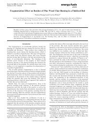
is repeated. Figure 5 illustrates in the right side the result
of applying this technique, although we only included
some threshold values for demonstration proposes.
As we may observe, with low threshold levels
we are able to isolate vertebrae with low intensity
(typically at the cervical) and with higher threshold
levels we accomplish to detect vertebrae with higher
intensity.
Figure 5: Detecting nodes along the spine (thresholds
from left to right: 32, 48, 176, and 192)
Nevertheless, this algorithm has two issues that
must be solved in order to correctly divide the spine
into vertebrae: (i) vertebrae may become shorter and
shorter while incrementing the threshold, and (ii) vertebrae
may be divided in several smaller regions due
to intensity variations along vertebrae. For handling
these problems we decided to use a tree data structure
to store the regions that the algorithm detects.
Every time a new region is found, it is added to the
tree as a child of the smallest region that entirely encloses
the new region. In order to control the tree size
and to overcome the problem (i), before increasing the
threshold to search for new regions, we prune the tree
by removing the leafs which have no siblings. Leafs
with no siblings are not interesting because they do
not divide the parent region. At most, they reduce the
size of the parent region which is not interesting because
vertebrae should have maximum height in order
to stay close to each other. By the end of the algorithm,
the tree is fully constructed and its leafs should
represent vertebrae, unless some vertebrae were overdivided.
For detecting over-divided vertebrae we do
two tests: (i) we check if the gaps between vertebrae
are not too large, and (ii) we determine if the vertebra
size is consistent with its adjacent vertebrae (e.g.
if it is not too small compared to its largest adjacent
vertebra). Whenever one of the previous situations is
detected, we test if the leaf’s parent is a better candidate
for that vertebra. If that is the case, we remove all
the leaf’s parent childes, transforming the parent into
a leaf and therefore in a vertebra.
2.3 Detecting vertebrae limits in the X axis
After detecting where the vertebrae are located along
the spine, we must detect where they start and end
along the X axis. This operation may be more difficult
than what it seems because part of the ribs may still
be attached to vertebrae in the processed image. This
happens when ribs also show high intensity levels and
the spine isolation method is not precise enough to get
rid of them.
For detecting vertebrae X limits we divide them in
several clusters along its width (currently we divide it
in 15 clusters). Then, we rank the clusters according
to their intensity levels. Intensity levels are calculated
using an exponential scale to give more preponderance
to very high levels. This allow us to distinguish
between clusters with high intensity structures surrounded
by low intensity pixels, and more homogeneous
clusters with average intensity levels. We then
select the first three clusters with more intensity and
we elect them as candidates for being the X limits.
One of these candidates will represent the start of the
vertebra and the other will represent the end. Initially,
the two more intense clusters are selected. Then, for
each vertebra, we compare its width and X centre with
its nearest 4 vertebrae. If we detect a considerable deviation
of the vertebra centre or an unexpected change
in width, we try different combinations of the three
candidate clusters and we select the ones that best fit
the conditions.
Finally, we optimise the results by finding inside
the elected clusters the largest concentration of bright
pixels. Only then the process of detecting the X limits
is completed. In Figure 6 we may see the nodes
4