Measuring Market Risk - Reserve Bank of India
Measuring Market Risk - Reserve Bank of India
Measuring Market Risk - Reserve Bank of India
Create successful ePaper yourself
Turn your PDF publications into a flip-book with our unique Google optimized e-Paper software.
<strong>Reserve</strong> <strong>Bank</strong> <strong>of</strong> <strong>India</strong> Occasional Papers<br />
Vol. 31, No.1, Summer 2010<br />
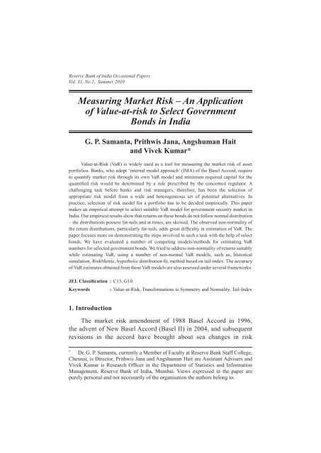
<strong>Measuring</strong> <strong>Market</strong> <strong>Risk</strong> – An Application<br />
<strong>of</strong> Value-at-risk to Select Government<br />
Bonds in <strong>India</strong><br />
G. P. Samanta, Prithwis Jana, Angshuman Hait<br />
and Vivek Kumar*<br />
Value-at-<strong>Risk</strong> (VaR) is widely used as a tool for measuring the market risk <strong>of</strong> asset<br />
portfolios. <strong>Bank</strong>s, who adopt ‘internal model approach’ (IMA) <strong>of</strong> the Basel Accord, require<br />
to quantify market risk through its own VaR model and minimum required capital for the<br />
quantified risk would be determined by a rule prescribed by the concerned regulator. A<br />
challenging task before banks and risk managers, therefore, has been the selection <strong>of</strong><br />
appropriate risk model from a wide and heterogeneous set <strong>of</strong> potential alternatives. In<br />
practice, selection <strong>of</strong> risk model for a portfolio has to be decided empirically. This paper<br />
makes an empirical attempt to select suitable VaR model for government security market in<br />
<strong>India</strong>. Our empirical results show that returns on these bonds do not follow normal distribution<br />
– the distributions possess fat-tails and at times, are skewed. The observed non-normality <strong>of</strong><br />
the return distributions, particularly fat-tails, adds great difficulty in estimation <strong>of</strong> VaR. The<br />
paper focuses more on demonstrating the steps involved in such a task with the help <strong>of</strong> select<br />
bonds. We have evaluated a number <strong>of</strong> competing models/methods for estimating VaR<br />
numbers for selected government bonds. We tried to address non-normality <strong>of</strong> returns suitably<br />
while estimating VaR, using a number <strong>of</strong> non-normal VaR models, such as, historical<br />
simulation, <strong>Risk</strong>Metric, hyperbolic distribution fit, method based on tail-index. The accuracy<br />
<strong>of</strong> VaR estimates obtained from these VaR models are also assessed under several frameworks.<br />
JEL Classification : C13, G10<br />
Keywords : Value-at-<strong>Risk</strong>, Transformations to Symmetry and Normality, Tail-Index<br />
1. Introduction<br />
The market risk amendment <strong>of</strong> 1988 Basel Accord in 1996,<br />
the advent <strong>of</strong> New Basel Accord (Basel II) in 2004, and subsequent<br />
revisions in the accord have brought about sea changes in risk<br />
*<br />
Dr. G. P. Samanta, currently a Member <strong>of</strong> Faculty at <strong>Reserve</strong> <strong>Bank</strong> Staff College,<br />
Chennai, is Director, Prithwis Jana and Angshuman Hait are Assistant Advisers and<br />
Vivek Kumar is Research Officer in the Department <strong>of</strong> Statistics and Information<br />
Management, <strong>Reserve</strong> <strong>Bank</strong> <strong>of</strong> <strong>India</strong>, Mumbai. Views expressed in the paper are<br />
purely personal and not necessarily <strong>of</strong> the organisation the authors belong to.
2 RESERVE BANK OF INDIA OCCASIONAL PAPERS<br />
management framework adopted at banks globally in recent years.<br />
Regulators across the world today follow banking supervision<br />
systems broadly similar to the framework articulated in these<br />
documents. A key feature <strong>of</strong> this framework is the risk capital – the<br />
minimum amount <strong>of</strong> capital a bank requires to keep for its exposure<br />
to risk. It is argued that the risk capital acts as a cushion against<br />
losses, protecting depositors’ interest and increasing the resilience <strong>of</strong><br />
the banking system in the event <strong>of</strong> crisis. <strong>Risk</strong> capital also makes the<br />
banks take risk on their own fund, thereby induces them to invest in<br />
prudent assets and curb their tendency to take excessive risk, which<br />
reduces the chances <strong>of</strong> bank runs greatly. So, the risk-based capital<br />
regulation has emerged as a tool to maintain stability <strong>of</strong> banking<br />
sector. Eventually, not only the banks but an increasing number<br />
<strong>of</strong> other financial institutions and firms are also aligning their risk<br />
management framework in the similar line.<br />
Two important changes are notable in the supervisory framework<br />
in recent years. First, determination <strong>of</strong> minimum required capital is<br />
now made more risk-sensitive (also more scientific) than earlier.<br />
Second, there has been an expansion in coverage <strong>of</strong> risk events in<br />
banks’ portfolio. In contrast to traditional focus solely on credit risk<br />
(BIS, 1988), the regulatory framework has gradually covered two<br />
more important risk categories, viz., market risk (BIS, 1996a, 1996b)<br />
and operational risk (BIS, 2004).<br />
The Basel Accords and associated amendments/revisions provide<br />
broad guidelines to determine the level <strong>of</strong> minimum required capital a<br />
bank should maintain for all three types <strong>of</strong> financial risks mentioned<br />
above. Under each risk category there have been a number <strong>of</strong> alternative<br />
approaches – starting from simple/basic to advanced in increasing level<br />
<strong>of</strong> sophistication. Also a distinction between basic and more advanced<br />
approach is that later emphasizes more on actual quantification <strong>of</strong> risk.<br />
In the case <strong>of</strong> ‘market risk’ the advanced approach is known as<br />
‘internal model approach’ (IMA), wherein risk capital is determined<br />
based on the new risk measure, called value-at-risk (VaR). Higher the<br />
value <strong>of</strong> VaR, higher the level <strong>of</strong> market risk, thereby; larger the level
MEASURING MARKET RISK 3<br />
<strong>of</strong> minimum required capital for market risk. <strong>Bank</strong>s, who adopt IMA,<br />
subject to regulators’ approval, would quantify market risk through its<br />
own VaR model and minimum required capital for the quantified risk<br />
would be determined by a rule prescribed by the concerned regulator.<br />
The concept <strong>of</strong> VaR was first introduced in the regulatory<br />
domain in 1996 (BIS, 1996) in the context <strong>of</strong> measuring market<br />
risk. However, post-1996 literature has given ample demonstration<br />
that the same concept is also applicable to much wider class <strong>of</strong><br />
risk categories, including credit and operational risks. Today, VaR<br />
is considered as a unified risk measure and a new benchmark for<br />
risk management. Interestingly, not only the regulators and banks<br />
but many private sector groups also have widely endorsed statisticalbased<br />
risk management systems, such as, VaR.<br />
As stated above, modern risk management practices at banks<br />
demand for proper assessment <strong>of</strong> risk and VaR concept is an influential<br />
tool for the purpose. The success <strong>of</strong> capital requirement regulation<br />
lies on determination <strong>of</strong> appropriate level <strong>of</strong> minimum required risk<br />
capital, which in turns depends on accuracy <strong>of</strong> quantified risk. There<br />
has been a plethora <strong>of</strong> approaches in measuring VaR from data, each<br />
having some merits over others but suffering from some inherent<br />
limitations. Also, each approach covers a number <strong>of</strong> alternative<br />
techniques which are sometimes quite heterogeneous. A challenging<br />
task before banks and risk managers, therefore, has been the selection<br />
<strong>of</strong> appropriate risk model from a wide and heterogeneous set <strong>of</strong><br />
potential alternatives. Ironically, theory does not help much in direct<br />
identification <strong>of</strong> the best suitable risk model for a portfolio.<br />
In practice, selection <strong>of</strong> risk model for a portfolio has to be<br />
based on empirical findings. Against this backdrop, this paper makes<br />
an empirical attempt to select VaR model for government security<br />
market in <strong>India</strong>. The paper focuses more on demonstrating the steps<br />
involved in such a task with the help <strong>of</strong> select bonds. In reality, actual<br />
portfolio differs (say, in terms <strong>of</strong> composition) across investors/<br />
banks and the strategy demonstrated here can be easily replicated for<br />
any specific portfolio. The rest <strong>of</strong> the paper is organized as follows.
4 RESERVE BANK OF INDIA OCCASIONAL PAPERS<br />
Section 2 presents the VaR concept and discusses some related issues.<br />
Section 3 summarises a number <strong>of</strong> techniques to estimate VaR using<br />
historical returns for a portfolio and Section 4 discusses criteria to<br />
evaluate alternative VaR models. Empirical results for select bonds<br />
are presented in Section 5. Finally, Section 6 presents the concluding<br />
remarks <strong>of</strong> the paper.<br />
Section II<br />
Value-at-<strong>Risk</strong> – The Concept, Usage and Relevant Issues<br />
2.1 Defining Value-at-<strong>Risk</strong><br />
The VaR is a number indicating the maximum amount <strong>of</strong> loss,<br />
with certain specified confidence level, a financial position may<br />
incur due to some risk events/factors, say, market swings (market<br />
risk) during a given future time horizon (holding period). If the<br />
value <strong>of</strong> a portfolio today is W, one can always argue that the entire<br />
value may be wiped out at some crisis phase so the maximum<br />
possible loss would be the today’s portfolio value itself. However,<br />
VaR does not refer to this trivial upper bound <strong>of</strong> the loss. The VaR<br />
concept is defined in a probabilistic framework, making it possible<br />
to determine a non-trivial upper bound (lower than trivial level) for<br />
loss at a specified probability. Denoting L to represent loss <strong>of</strong> the<br />
portfolio over a specified time horizon, the VaR for the portfolio, say<br />
V*, associated with a given probability, say p, 0 < p V*] = p, or equivalently, Prob[Loss < V*] = (1-p), where<br />
Prob[.] represents the probability measure. Usually, the terms ‘VaR<br />
for probability p’ refer to the definitional identity Prob[Loss > V*]<br />
= p, and the terms ‘VaR for 100*(1-p) per cent confidence level’ are<br />
used to refer to the identity Prob[Loss < V*] = (1-p).<br />
The VaR can be defined in terms <strong>of</strong> a threshold for change in value<br />
<strong>of</strong> the portfolio also. In order to illustrate this point, let W t<br />
denotes the<br />
total value <strong>of</strong> underlying assets corresponding to a financial position<br />
at time instance t, and the change in value <strong>of</strong> the position from time<br />
t to t+h is ∆W t<br />
(h) = (W t+h<br />
- W t<br />
). At time point t, W t+h<br />
is not known,<br />
so ∆W t<br />
(k) is also unknown and can be considered a random variable.<br />
So, the value-at-risk V* would satisfy the identity Prob[∆W t<br />
(h)
MEASURING MARKET RISK 5<br />
< -V*] = p, or equivalently, as earlier, the identity can be expressed<br />
as Prob[∆W t<br />
(h) > -V*] = (1-p).<br />
It is important to note that any VaR number has two parameters,<br />
viz., holding period (i.e. time horizon) and probability/confidence<br />
level. For a given portfolio, VaR number changes with these two<br />
parameters - while VaR decreases (increases) with the rise (fall) <strong>of</strong><br />
probability level 1 , it changes in the same direction with changes in<br />
holding period.<br />
2.2 Short and Long Financial Positions, and VaR<br />
The holder <strong>of</strong> a short financial position suffers a loss when the<br />
prices <strong>of</strong> underlying assets rise, and concentrates on upper-tail <strong>of</strong><br />
the distribution while calculating her VaR (Tsay, 2002, pp. 258).<br />
Similarly, the holder <strong>of</strong> a long financial position would model the<br />
lower-tail <strong>of</strong> return distribution as a negative return on underlying<br />
assets makes her suffer a loss.<br />
2.3 Usage <strong>of</strong> VaR<br />
Despite being a single number for a portfolio, VaR has several<br />
usages. First, VaR itself is a risk measure. Given probability level<br />
‘p’ and holding period, larger VaR number would indicate greater<br />
risk in a portfolio. Thus, VaR has ability to rank portfolios in order<br />
<strong>of</strong> risk. The second, it gives a numerical maximal loss (probabilistic)<br />
for a portfolio. Unlike other common risk measures, this is an<br />
additional advantage in measuring risk through VaR concept. Third,<br />
VaR number is useful to determine the regulatory required capital for<br />
banks exposure to risk.<br />
Apart from the general usages <strong>of</strong> VaR concept, it is also<br />
worthwhile to note a few points on its applicability to various risk<br />
categories. Though there has been criticism against it as being not a<br />
coherent risk measure and lacking some desirable properties (see for
6 RESERVE BANK OF INDIA OCCASIONAL PAPERS<br />
instance, Artzner, et al., 1999), it is a widely accepted risk measure<br />
today. Though VaR was originally endorsed as a tool to measure<br />
market risk, it provides a unified framework to deal with other risks,<br />
such as, credit risk, operation risk. As seen in the definition, the<br />
essence <strong>of</strong> VaR is that it is a percentile <strong>of</strong> loss/return distribution<br />
for a portfolio. So long as one has data to approximate/fit the loss<br />
distribution, VaR being a characteristic <strong>of</strong> such distribution, can be<br />
estimated from the fitted distribution.<br />
2.4 Choice <strong>of</strong> Probability Level and Holding Period<br />
The choice <strong>of</strong> ‘probability/confidence level’ and ‘holding period’<br />
would depend on the purpose <strong>of</strong> estimating the VaR measure. It is now<br />
a common practice, as also prescribed by the regulators, to compute<br />
VaR for probability level 0.01, i.e. 99% confidence level. In addition,<br />
researchers sometimes consider assessment <strong>of</strong> risk for select other<br />
probability levels, such as, for probability 0.05.<br />
A useful guideline for deciding ‘holding period’, is the liquidation<br />
period – the time required to liquidate a portfolio 2 . An alternative<br />
view is that the holding period would represent the ‘period over<br />
which the portfolio remains relatively stable’. Holding period may<br />
also relates to the time required to hedge the risk. Notably, a rise in<br />
holding period will increase the VaR number. One may also get same<br />
outcome by reducing probability level (i.e. increasing confidence<br />
level) adequately (instead <strong>of</strong> changing holding period). In practice,<br />
regulators maintain uniformity in fixing probability level at p=0.01<br />
(equivalently, 99% confidence level). Thus, holding period has to be<br />
decided based on some <strong>of</strong> the consideration stated above. It may be<br />
noted that VaR for market risk may have much shorter holding period<br />
as compared to say VaR for credit risk. Basel Accords suggests 10-<br />
day holding period for market risk, though country regulators may<br />
prescribe higher holding period. In case <strong>of</strong> credit risk, duration <strong>of</strong><br />
holding period is generally one-year.
MEASURING MARKET RISK 7<br />
2.5 VaR Expressed in Percentage and Other Forms<br />
As seen, VaR is defined in terms <strong>of</strong> the change/loss in value<br />
<strong>of</strong> a portfolio. In practice, distribution <strong>of</strong> return (either percentage<br />
change or continuously-compounded/log-difference 3 ) <strong>of</strong> the financial<br />
position may actually be modeled and thus, VaR may be estimated<br />
based on percentile <strong>of</strong> the underlying return distribution. Sometimes<br />
percentiles <strong>of</strong> return distribution are termed as ‘relative VaR’ (see for<br />
instance, Wong, et al., 2003). On this perception, the VaR for change<br />
in value may be termed as ‘absolute/nominal VaR’.<br />
Thus, the percentile ξ p<br />
corresponding to left-tail probability p <strong>of</strong><br />
distribution <strong>of</strong> k-period percentage change itself is the relative VaR<br />
(expressed in per cent) with specified parameters and corresponding<br />
(absolute) VaR would be [(ξ p<br />
/100)W t<br />
]. Alternatively, if ξ p<br />
represents<br />
the p-percentile for log-return (in per cent), then (absolute) VaR can be<br />
expressed as [{exp(ξ p<br />
/100)-1}W t<br />
]. In our paper, unless otherwise stated,<br />
we use the term VaR to indicate ‘relative VaR’ (expressed in per cent).<br />
2.6 The h-period VaR from 1-period VaR<br />
Another point to be noted relates to the estimation <strong>of</strong> multiperiod<br />
VaR (i.e. VaR corresponding to multi-period ‘time horizon’,<br />
say h-day). In practice, given probability level ‘p’, 0
8 RESERVE BANK OF INDIA OCCASIONAL PAPERS<br />
for simplicity, this has been widely used in practice and regulators<br />
across the world has also subscribed to such approximation. Indeed,<br />
as per the regulators’ guidelines, banks adopting IMA for market risk<br />
require to compute 1-day VaR using daily returns and the validation<br />
<strong>of</strong> risk-model depends upon how accurately the models estimate<br />
1-day VaR. However, minimum required capital is determined using<br />
multi-period VaR, say 10-day VaR numbers, which are generated<br />
from the 1-day VaR values.<br />
Section III<br />
Measurement <strong>of</strong> VaR – Select Techniques<br />
The central to any VaR measurement exercise has been the<br />
estimation <strong>of</strong> suitable percentile <strong>of</strong> change in value or return <strong>of</strong> the<br />
portfolio. Following the earlier discussion, we focus here in estimating<br />
1-period VaR (e.g., 1-day VaR using daily returns). Also, we shall be<br />
focusing only on estimating VaR directly from portfolio-level returns.<br />
As well known, a portfolio usually consists <strong>of</strong> several securities and<br />
financial instruments/assests, and returns on each component <strong>of</strong> the<br />
portfolio would follow certain probability distribution. Portfolio<br />
value is the weighted sum <strong>of</strong> all components, changes in which can<br />
be assessed by studying the multivariate probability distribution<br />
considering returns on all components <strong>of</strong> the portfolio. In our study,<br />
such a strategy has not been followed. Instead, our analysis, as quite<br />
common in the literature, relies on historical portfolio-level returns<br />
and VaR estimation essentially requires to study the underlying<br />
univariate distribution.<br />
3.1 Estimating VaR Under Normality <strong>of</strong> Unconditional Return<br />
Distribution<br />
The normality assumption to portfolio return distribution<br />
simplifies the task <strong>of</strong> VaR estimation greatly. A normal distribution is<br />
fully characterized by first two moments, viz., mean (µ) and standard
MEASURING MARKET RISK 9<br />
deviation (σ), and the percentile with left-tail probability p, 0
10 RESERVE BANK OF INDIA OCCASIONAL PAPERS<br />
extreme value theory (EVT) - modeling either the distribution <strong>of</strong><br />
extreme return or only the tails <strong>of</strong> return distribution.<br />
3.2.1 Non-Parametric Approach - Historical Simulation<br />
The non-parametric approach, such as, historical simulation (HS),<br />
possess some specific advantages over the normal method, as it is<br />
not model based, although it is a statistical measure <strong>of</strong> potential loss.<br />
The main benefit is that it can cope with all portfolios that are either<br />
linear or non-linear. The method does not assume any specific form<br />
<strong>of</strong> the distribution <strong>of</strong> price change/return. The method captures the<br />
characteristics <strong>of</strong> the price change distribution <strong>of</strong> the portfolio, as it<br />
estimates VaR based on the distribution actually observed. But one<br />
has to be careful in selecting past data. If the past data do not contain<br />
highly volatile periods, then HS method would not be able to capture<br />
the same. Hence, HS should be applied when one has very large data<br />
points to take into account all possible cyclical events. HS method<br />
takes a portfolio at a point <strong>of</strong> time and then revalues the same using<br />
the historical price series. Daily returns, calculated based on the price<br />
series, are then sorted in an ascending order and find out the required<br />
data point at desired percentiles. Linear interpolation can be used to<br />
estimate required percentile if it falls in between two data points.<br />
Another variant <strong>of</strong> HS method is a hybrid approach put forward<br />
by Boudhoukh, et al. (1997), that takes into account the exponentially<br />
weighing approach in HS for estimating the percentiles <strong>of</strong> the return<br />
directly. As described by Boudhoukh et al. (1997, pp. 3), “the<br />
approach starts with ordering the returns over the observation period<br />
just like the HS approach. While the HS approach attributes equal<br />
weights to each observation in building the conditional empirical<br />
distribution, the hybrid approach attributes exponentially declining<br />
weights to historical returns”. The process is simplified as follows:<br />
<br />
Calculate the return series <strong>of</strong> past price data <strong>of</strong> the security or the<br />
portfolio.<br />
Fix a value δ from the interval (0,1). Usually δ is fixed at =0.98.<br />
<br />
To each most recent k returns: R(t), R(t-1), …R(t-k+1) assign a
MEASURING MARKET RISK 11<br />
weight proportional to 1, δ, δ 2 , …., δ k-1 , respectively. In order to make<br />
total weights sum to 1, the weights for R(t), R(t-1), …..,R(t-k+1)<br />
would be ,<br />
respectively 4 .<br />
<br />
Sort the returns in ascending order.<br />
<br />
In order to obtain VaR <strong>of</strong> the portfolio for probability ‘p’, 0
12 RESERVE BANK OF INDIA OCCASIONAL PAPERS<br />
where and , respectively, denote estimated conditional mean<br />
and variance for time point t+1 (using information upto time t) 5 .<br />
There exist several alternative models to estimate conditional<br />
mean and variance. The simplest form <strong>of</strong> conditional heteroscedastic<br />
model is the one like exponentially weighted moving average as used<br />
in <strong>Risk</strong>Metrics (J.P. Morgan/Reuters, 1996). This popular technique<br />
in effect models conditional variance as a weighted average <strong>of</strong> past<br />
variances and past returns, where exponential weighting scheme for<br />
past returns is used as follows;<br />
....(4)<br />
where and r t<br />
denote conditional variance and return at time t,<br />
respectively; denotes the variance at origin (i.e. time t=0); and the<br />
parameter λ, known as decay factor, satisfies 0 < λ
MEASURING MARKET RISK 13<br />
distributional forms considered would be quite wide including, say,<br />
hyperbolic distribution, t-distribution, mixture <strong>of</strong> two or more normal<br />
distributions, Laplace distribution or so forth, (van den Goorbergh<br />
and Vlaar, 1999; Bauer 2000; Linden, 2001).<br />
In our study we consider symmetric hyperbolic distribution as an<br />
alternative fat-tailed distribution for returns 6 . A d-dimensional random<br />
variable ‘r’ is said to follow a symmetric hyperbolic distribution if it<br />
has density function as below;<br />
where, K ν<br />
is the modified Bessel function <strong>of</strong> the third kind, the<br />
parameters δ and ∆ are for multivariate scales, µ for location and ζ<br />
mainly changes the tails.<br />
For the presence <strong>of</strong> Bessel functions in above density function,<br />
closed form expression for maximum likelihood estimators are not<br />
possible. Bauer (2000) suggests an approach to have maximum<br />
likelihood estimators 7 . Once estimates <strong>of</strong> the parameters become<br />
available, one can estimate the required percentile <strong>of</strong> the distribution<br />
following numerical iteration method.<br />
3.2.4 Methods under Extreme Value Theory – Use <strong>of</strong> Tail-Index<br />
The fat tails <strong>of</strong> unconditional return distribution can also be<br />
handled through extreme value theory using, say, tail-index, which<br />
measures the amount <strong>of</strong> tail fatness. One can therefore, estimate the<br />
tail-index and measure VaR based on the underlying distribution. The<br />
basic premise <strong>of</strong> this idea stems from the result that the tails <strong>of</strong> every<br />
fat-tailed distribution converge to the tails <strong>of</strong> Pareto distribution. In a<br />
simple case, upper tail <strong>of</strong> such a distribution can be modeled as,
14 RESERVE BANK OF INDIA OCCASIONAL PAPERS<br />
Prob[X > x] ≈ C α |x| –α (i.e. Prob[X ≤ x] ≈ 1 - C α |x| -α ); x>C ….. (6)<br />
Where, C is a threshold above which the Pareto law holds; |x| denotes<br />
the absolute value <strong>of</strong> x and the parameter α is the tail-index.<br />
Similarly, lower tail <strong>of</strong> a fat-tailed distribution can be modeled as<br />
Prob[X > x] ≈1 - C α x –α (i.e. Prob[X ≤ x] ≈ C α x -α ); x < C ….. (7)<br />
Where, C is a threshold below which the Pareto law holds, and the<br />
parameter α, called as tail-index, measures the tail-fatness.<br />
In practice, observations in upper tail <strong>of</strong> the return distribution<br />
are generally positive and those in lower tail are negative. The holder<br />
<strong>of</strong> a short financial position suffers a loss in the event <strong>of</strong> a rise in<br />
values <strong>of</strong> underlying assets and therefore, concentrates on upper-tail<br />
<strong>of</strong> the distribution (i.e. Eqn. 6) for calculating VaR (Tsay, 2002, pp.<br />
258). Similarly, the holder <strong>of</strong> a long financial position would model<br />
the lower-tail <strong>of</strong> the underlying distribution (i.e. use Eqn. 7) as a fall<br />
in asset values makes her suffer a loss.<br />
From Eqns.(6) and (7), it is clear that the estimation <strong>of</strong> VaR is<br />
crucially dependent on the estimation <strong>of</strong> tail-index α. There are several<br />
methods <strong>of</strong> estimating tail-index, such as, (i) Hill’s (1975) estimator<br />
and (ii) the estimator under ordinary least square (OLS) framework<br />
suggested by van den Goorbergh and Vlaar (1999). In this study, only<br />
the widely used Hill’s estimator <strong>of</strong> tail-index is considered.<br />
Section IV<br />
Selecting VaR Model – Evaluation Criteria<br />
The accuracy <strong>of</strong> VaR estimates obtained from a VaR model<br />
can be assessed under several frameworks, such as, (i) regulators’<br />
backtesting (henceforth simply called as backtesting); (ii) Kupiec’s<br />
test; (iii) loss-function based evaluation criteria. Under each<br />
framework, there would be several techniques and what follows is<br />
the summary <strong>of</strong> some <strong>of</strong> the widely used techniques.
MEASURING MARKET RISK 15<br />
4.1 Backtesting<br />
As recommended by Basel Committee, central banks do not<br />
specify any VaR model to the banks. Rather under the advanced<br />
‘internal model approach’, banks are allowed to adopt their own<br />
VaR model. There is an interesting issue here. As known, VaR is<br />
being used for determining minimum required capital – larger the<br />
value <strong>of</strong> VaR, larger is the capital charge. Since larger capital charge<br />
may affect pr<strong>of</strong>itability adversely, banks have an incentive to adopt<br />
a model that produces lower VaR estimate. In order to eliminate<br />
such inherent inertia <strong>of</strong> banks, Basel Committee has set out certain<br />
requirements on VaR models used by banks to ensure their reliability<br />
(Basel Committee, 1996a,b) as follows;<br />
(i) 1-day and 10-day VaRs must be estimated based on the daily<br />
data <strong>of</strong> at least one year<br />
(ii) Capital charge is equal to three times the 60-day moving average<br />
<strong>of</strong> 1% 10-day VaRs, or 1% 10-day VaR on the current day, which<br />
ever is higher. The multiplying factor (here 3) is known as<br />
‘capital multiplier’.<br />
Further, Basel Committee (1996b) provides following Backtesting<br />
criteria for an internal VaR model (see van den Goorbergh and Vlaar,<br />
1999; Wong et al., 2003, among others)<br />
(i) One-day VaRs are compared with actual one-day trading<br />
outcomes.<br />
(ii) One-day VaRs are required to be correct on 99% <strong>of</strong> backtesting<br />
days. There should be at least 250 days (around one year) for<br />
backtesting.<br />
(iii) A VaR model fails in Backtesting when it provides 5% or more<br />
incorrect VaRs.<br />
If a bank provides a VaR model that fails in backtesting, it will<br />
have its capital multiplier adjusted upward, thus increasing the amount<br />
<strong>of</strong> capital charges. For carrying out the Backtesting <strong>of</strong> a VaR model,<br />
realized day-to-day returns <strong>of</strong> the portfolio are compared to the VaR <strong>of</strong>
16 RESERVE BANK OF INDIA OCCASIONAL PAPERS<br />
the portfolio. The number <strong>of</strong> days, when actual portfolio loss is higher<br />
than VaR estimate, provides an idea about the accuracy <strong>of</strong> the VaR<br />
model. For a good 99% VaR model, this number would approximately<br />
be equal to the 1 per cent (i.e. 100 times <strong>of</strong> VaR probability) <strong>of</strong> backtesting<br />
days. If the number <strong>of</strong> VaR violations or failures (i.e. number <strong>of</strong><br />
days when observed loss exceeds VaR estimate) is too high, a penalty is<br />
imposed by raising the multiplying factor (which is at least 3), resulting<br />
in an extra capital charge. The penalty directives provided by the Basel<br />
Committee for 250 back-testing trading days is as follows; multiplying<br />
factor remains at minimum (i.e. 3) for number <strong>of</strong> violations up to 4,<br />
increases to 3.4 for 5 violations, 3.5 for 6 violations, 3.65 for violations<br />
7, 3.75 for violations 8, 3.85 for violations 9, and reaches at 4.00 for<br />
violations above 9 in which case the bank is likely to be obliged to<br />
revise its internal model for risk management (van den Goorbergh and<br />
Vlaar, 1999).<br />
4.2 Statistical Tests <strong>of</strong> VaR Accuracy<br />
The accuracy <strong>of</strong> a VaR model can also be assessed statistically by<br />
applying Kupiec’s (1995) test (see, for example, van den Goorbergh<br />
and Vlaar, 1999 for an application <strong>of</strong> the technique). The idea behind<br />
this test is that frequency <strong>of</strong> VaR- violation should be statistically<br />
consistent with the probability level for which VaR is estimated.<br />
Kupiec (1995) proposed to use a likelihood ratio statistics for testing<br />
the said hypothesis.<br />
If z denotes the number <strong>of</strong> times the portfolio loss is worse than the<br />
VaR estimate in the sample (<strong>of</strong> size T, say) then z follows a Binomial<br />
distribution with parameters (T, p), where p is the probability level<br />
<strong>of</strong> VaR. Ideally, more the z/T closes to p, more accurate the estimated<br />
VaR is. Thus the null hypothesis z/T = p may be tested against the<br />
alternative hypothesis z/T ≠ p. The likelihood ratio (LR) statistic for<br />
testing the null hypothesis against the alternative hypothesis is<br />
….. (8)
MEASURING MARKET RISK 17<br />
Under the null hypothesis, LR-statistic follows a χ 2 -distribution<br />
with 1-degree <strong>of</strong> freedom.<br />
The VaR estimates are also interval forecasts, which thus, can<br />
be evaluated conditionally or unconditionally. While the conditional<br />
evaluation considers information available at each time point, the<br />
unconditional assessment is made without reference to it. The test<br />
proposed by Kupiec provides only an unconditional assessment as it<br />
simply counts violations over the entire backtesting period (Lopez,<br />
1998). In the presence <strong>of</strong> time-varying volatility, the conditional<br />
accuracy <strong>of</strong> VaR estimates assumes importance. Any interval forecast<br />
ignoring such volatility dynamics may have correct unconditional<br />
coverage but at any given time, may have incorrect conditional<br />
coverage. In such cases, the Kupiec’s test has limited use as it may<br />
classify inaccurate VaR as acceptably accurate.<br />
A three-step testing procedure developed by Christ<strong>of</strong>fersen (1998)<br />
involves a test for correct unconditional coverage (as Kupiec’s test),<br />
a test for ‘independence’, and a test for correct ‘conditional coverage’<br />
(Christ<strong>of</strong>fersen, 1998; Berkowitz and O’Brien, 2002; Sarma, et al.,<br />
2003). All these tests use Likelihood-Ratio (LR) statistics.<br />
4.3 Evaluating VaR Models Using Penalty/Loss-Function<br />
Tests mentioned above assess the frequency <strong>of</strong> VaR violations,<br />
either conditionally or unconditionally, during the backtesting trading<br />
days. These tests, however, do not look at the severity/magnitude<br />
<strong>of</strong> additional loss (i.e. loss in excess <strong>of</strong> estimated VaR) at the time<br />
<strong>of</strong> VaR violations. However, a portfolio manager may prefer the<br />
case <strong>of</strong> more frequent but little additional loss than the case <strong>of</strong> less<br />
frequent but huge additional loss. The underlying VaR model in the<br />
former case may fail in backtesting but still the total amount <strong>of</strong> loss<br />
(after adjusting for penalty on multiplying factor, if any) during the<br />
backtesting trading days may be less than that in later case. So long<br />
as this condition persists with a VaR model, a portfolio manager,<br />
particularly non-banks who are not required to comply with any<br />
regulatory requirement, may prefer to accept the VaR model even
18 RESERVE BANK OF INDIA OCCASIONAL PAPERS<br />
if it fails in backtesting. This means that the objective function <strong>of</strong> a<br />
portfolio manager is not necessarily be the same as that provided by<br />
the backtesting. Each manager may set his own objective function and<br />
try to optimize that while managing market risk. But, loss-functions<br />
<strong>of</strong> individual portfolio managers are not available in public domain<br />
and thus, it would be impossible to select a VaR model appropriate<br />
for all managers. However, discussion on a systematic VaR selection<br />
framework by considering a few specific forms <strong>of</strong> loss-function<br />
would provide insight into the issue so as to help individual manager<br />
to select a VaR model on the basis <strong>of</strong> his own loss-function. On this<br />
perception, it would be interesting to illustrate the VaR selection<br />
framework with the help <strong>of</strong> some specific forms <strong>of</strong> loss-function.<br />
The idea <strong>of</strong> using loss-function for selecting VaR model, perhaps,<br />
is proposed first by Lopez (1998). He shows that the binomial<br />
distribution-based test is actually minimizing a typical loss-function<br />
– gives score 1 for a VaR violation and a score 0 otherwise. In other<br />
words, the implied loss-function in backtesting would be an indicator<br />
function I t<br />
which assumes a value 1 at time t if the loss at t exceeds<br />
corresponding VaR estimate and assumes a value zero otherwise.<br />
However, it is hard to imagine an economic agent who has such a utility<br />
function: one which is neutral to all times with no VaR violation and<br />
abruptly shifts to score <strong>of</strong> 1 in the slightest failure and penalizes all<br />
failures equally (Sarma, et al., 2003). Lopez (1998) also considers a<br />
more generalised loss-function which can incorporate the regulatory<br />
concerns expressed in the multiplying factor and thus is analogous<br />
to the adjustment schedule for the multiplying factor for determining<br />
required capital. But, he himself observed that, like the simple<br />
binomial distribution-based loss-function, this loss-function is also<br />
based on only the number <strong>of</strong> violations in backtesting observations –<br />
with paying no attention to another concern, the magnitudes <strong>of</strong> loss<br />
at the time <strong>of</strong> failures. In order to handle this situation, Lopez (1998)<br />
also proposes a different loss-function addressing the magnitude <strong>of</strong><br />
violation as follows;<br />
..... (9)
MEASURING MARKET RISK 19<br />
where L t<br />
denotes a score at time t, Loss t<br />
is the magnitude/amount <strong>of</strong><br />
loss at time t and VaR t|t-1<br />
is the estimated value-at-risk made for time<br />
t made at time (t-1).<br />
The overall score (i.e. value <strong>of</strong> the loss-function) is the<br />
summation <strong>of</strong> all scores (L t<br />
) over all back testing days. A VaR<br />
model which gives minimum overall score is preferred over other<br />
competing models.<br />
In the spirit <strong>of</strong> Lopez (1998), Sarma et al. (2003) consider two<br />
loss-functions, viz., regulatory loss function and the firm’s loss<br />
function, which assign scores on t-th backtesting day as follows;<br />
Regulatory Loss Function<br />
Firm’s Loss Function<br />
..... (10)<br />
..... (11)<br />
where α represents the opportunity cost <strong>of</strong> capital and meaning <strong>of</strong><br />
other symbols and variables are as above.<br />
Empirical Results<br />
5.1 Data<br />
Section V<br />
Data availability in government securities to carry out value-atrisk<br />
analy sis is quite difficult. This is simply because the government<br />
securities market is still not vibrant, deep and liquid enough.<br />
Securities keep on changing their tradability making it difficult to<br />
get time series trade data on a particular security for more than, say,<br />
three years. One can easily verify that though there are more than<br />
ninety outstanding government securities, less than ten securities are<br />
traded for good volume or number <strong>of</strong> trade. Among these, <strong>of</strong> course,<br />
all are not regularly traded. We could get data for three years from
20 RESERVE BANK OF INDIA OCCASIONAL PAPERS<br />
August 2005 to July 2008. Effective working days during this three<br />
year period was 747 days while the most regularly traded security,<br />
8.07% GS 2017, during this period was traded for 685 days followed<br />
by 7.37% GS 2014 for 608 days. Even after having a Primary<br />
Dealers system in place, who are specifically treated as market<br />
maker, representative quotes or data on that in several government<br />
securities are not available. In such a scenario, the analysis was kept<br />
limited to the trade data <strong>of</strong> above mentioned two securities. In case<br />
any <strong>of</strong> these securities is not traded in a particular day, the price<br />
has been taken from what is disseminated by Fixed Income Money<br />
<strong>Market</strong> and Derivatives Association <strong>of</strong> <strong>India</strong> (FIMMDA) on a daily<br />
basis.<br />
5.2 Return Series<br />
For each chosen bond, we consider the continuously compounded<br />
daily returns computed as follows;<br />
R t<br />
= log e<br />
(P t<br />
) – log e<br />
(P t-1<br />
) ….. (12)<br />
Where P t<br />
and R t<br />
denote the price/value and return in t-th day.<br />
Using the price data for 747 days, we have returns on each<br />
bond for 746 days. The daily returns, plotted in Chart 1, clearly
MEASURING MARKET RISK 21<br />
exhibits volatility clustering indicating the fat-tails <strong>of</strong> unconditional<br />
distribution <strong>of</strong> returns. Observed probability distribution for each<br />
return series also appears to be non-normal (Chart 2).<br />
In order to formally examine whether returns follow normal<br />
distribution, we employed Jarque-Bera (1987) and two other related<br />
Chi-Square tests. The Jarque-Bera (1987) 8 test statistics is given by<br />
Q = n[ (b 1<br />
) 2 /6 + (b 2<br />
) 2 /24], where b 1<br />
and b 2<br />
are sample estimates<br />
<strong>of</strong> measure <strong>of</strong> skewness β 1<br />
and excess-kurtosis β 2<br />
, respectively and<br />
n is the number <strong>of</strong> observation used to derive the said estimates.<br />
Under the hypothesis <strong>of</strong> normality <strong>of</strong> return distribution, Q is<br />
asymptotically a χ 2 variable with 2 degrees <strong>of</strong> freedom. Also, under<br />
normality, each <strong>of</strong> b 1<br />
and b 2<br />
is asymptotically normally distributed<br />
with mean zero and respective variances 6/n and 24/n implying that<br />
each <strong>of</strong> [n (b 1<br />
) 2 /6] and [n (b 2<br />
) 2 /24] is asymptotically χ 2 variable with<br />
1 degree <strong>of</strong> freedom. The test statistics stated above are used to<br />
examine normality.<br />
Results <strong>of</strong> normality tests are presented in Table 1. As can be<br />
seen from this table, the Jarque-Bera test statistics is significant at
22 RESERVE BANK OF INDIA OCCASIONAL PAPERS<br />
Table 1: Testing Normality <strong>of</strong> Returns<br />
Govt. Bond<br />
Measure<br />
<strong>of</strong><br />
Skewness<br />
χ 2 1<br />
χ 2 1<br />
for<br />
Skewness<br />
Excess<br />
Kurtosis<br />
for<br />
Excess<br />
Kurtosis<br />
Jarque-Bera<br />
Statistics<br />
8.07%<br />
GS 2017<br />
-0.74 68.55*<br />
(0.0000)<br />
8.15 2066.82*<br />
(0.0000)<br />
2135.37*<br />
(0.0000)<br />
7.37% GS<br />
2014<br />
-0.15 2.71<br />
(0.0991)<br />
9.16 2609.94*<br />
(0.0000)<br />
2612.66*<br />
(0.0000)<br />
Note: Figures within ( ) indicate significance level (i.e. p-value) <strong>of</strong> corresponding statistics;<br />
‘*’ indicates significant at 1% level <strong>of</strong> significance.<br />
1% level <strong>of</strong> significance indicating that none <strong>of</strong> the return series<br />
could be considered to be normally distributed. The Chi-square<br />
tests for skewness or excess-kurtosis alone also support the finding.<br />
Results on these tests suggest that the underlying return distributions<br />
have significant excess-kurtosis indicating presence <strong>of</strong> fat-tails in the<br />
distributions and are skewed, though the degree <strong>of</strong> asymmetry in the<br />
case <strong>of</strong> the bond 7.37% GS 2014 appears to be mild 9 .<br />
5.3 VaR Estimates from Alternative Techniques<br />
The identified non-normality <strong>of</strong> the underlying return<br />
distributions poses a great difficulty in estimating value-at-risk. As<br />
discussed earlier, there have been a plethora <strong>of</strong> techniques to handle<br />
non-normality but hardly any theory can directly identify the best<br />
VaR technique for a given portfolio. Thus selecting VaR model is a<br />
decision-making problem that has to be addressed empirically. Our<br />
strategy in this regard is that estimate VaR using a set <strong>of</strong> alternative<br />
techniques/models and evaluate each competing model based on<br />
suitable criteria.<br />
In this study, 'normal method' is taken as the benchmark VaR<br />
estimation technique. The list <strong>of</strong> alternative approaches to handle<br />
non-normality includes (i) historical simulation – both simple and
MEASURING MARKET RISK 23<br />
hybrid; (ii) <strong>Risk</strong>Metric approach – using exponentially weighted sum<br />
<strong>of</strong> squares <strong>of</strong> past returns to capture the conditional heteroscedasticity<br />
in returns; (iii) symmetric hyperbolic distribution – a distribution<br />
having fat-tails; and (iv) tail-index based method – an approach<br />
under extreme value theory that measure tail fatness (through tailindex)<br />
and model tails <strong>of</strong> return distribution.<br />
As seen earlier, the hybrid/weighted form <strong>of</strong> historical simulation<br />
approach requires a parameter δ, 0 < δ < 1, which determines the<br />
weights <strong>of</strong> past returns while estimating volatility or VaR. As δ takes<br />
a fraction value, sometimes fixed at 0.98, the weight decays to with<br />
the increase in the remoteness <strong>of</strong> the past observation/return. We<br />
consider three alternative value <strong>of</strong> δ, viz., 0.94, 0.96 and 0.98.<br />
For implementing <strong>Risk</strong>Metric approach also, there is a need<br />
to fix a value for the parameter λ. In original <strong>Risk</strong>Metric approach,<br />
value <strong>of</strong> this parameter was fixed at 0.94. In this study, however, three<br />
alternatives values for λ, viz., 0.94, 0.96 and 0.98 are considered.<br />
Table 2 presents estimated 1-day VaRs, with probability level<br />
0.01 (i.e. 99% confidence level), obtained by applying chosen<br />
Table 2: Estimated VaR in the Last Day <strong>of</strong> the Database<br />
VaR Technique<br />
Security<br />
8.07% GS<br />
2017<br />
7.37% GS<br />
2014<br />
Normal – Benchmark Model 0.83 0.70<br />
Historical Simulation - Simple 1.11 0.90<br />
Historical Simulation – Hybrid/Weighted<br />
λ = 0.94 2.08 1.66<br />
λ = 0.96 2.08 1.66<br />
λ = 0.98 2.08 1.66<br />
<strong>Risk</strong> Metrics<br />
λ = 0.94 1.57 1.13<br />
λ = 0.96 1.75 1.43<br />
λ = 0.98 1.81 1.64<br />
Hyperbolic Distribution 1.15 0.96<br />
Tail Index 1.35 1.16
24 RESERVE BANK OF INDIA OCCASIONAL PAPERS<br />
alternative techniques for the last day in our database. Noting that<br />
returns do not follow normal distribution, VaR number is likely to<br />
be underestimated by normal method. Our empirical results are<br />
consistent on this matter. As can be seen from Table 2, VaR estimates<br />
obtained from normal method are the lowest for selected bonds 10 .<br />
Among the non-normal alternatives, historical simulation<br />
(simple) and hyperbolic distribution produces the lowest VaR<br />
numbers. On the other hand, the <strong>Risk</strong>Metric and hybrid historical<br />
simulation methods produce the highest VaR estimates. The tailindex<br />
based method results into VaR estimates some where in between<br />
these two sets <strong>of</strong> estimates.<br />
5.4 Evaluation <strong>of</strong> Competing VaR Models<br />
Competing VaR models were evaluated in terms <strong>of</strong> their<br />
accuracy in estimating VaR over last 447 days in the database. For<br />
each VaR model, we followed following steps: First, estimate 1-day<br />
VaR with 99% confidence level (i.e. probability level 0.01) using the<br />
returns for first 300 days. This estimate is then compared with the<br />
loss on 301 st day. In case loss exceeds VaR, we say that an instance<br />
<strong>of</strong> VaR-violation has occurred. Second, estimate VaR for 302 nd day<br />
using returns for past 300 days (covering the period from 2 nd to 301 st<br />
days). This estimate is then compared with the loss in 302 nd day in<br />
the database to see whether any VaR-violation occurred. Third, the<br />
process is repeated until all data points are exhausted. Finally, count<br />
the number/percentage <strong>of</strong> VaR violation over the period <strong>of</strong> 447 days.<br />
For a good VaR model, percentage <strong>of</strong> VaR violation should be equal<br />
to the theoretical value 1% (corresponding with probability level 0.01<br />
<strong>of</strong> estimated VaR numbers). In Table 3, the number/percentage <strong>of</strong><br />
VaR violation over last 447 days in the database is given separately<br />
for each <strong>of</strong> the competing VaR models.<br />
As can be seen from Table 3, percentage <strong>of</strong> VaR violation for<br />
the benchmark model ‘normal method’ is above 3% - far above
MEASURING MARKET RISK 25<br />
Table 3: Number (Percentage) <strong>of</strong> VaR Violation*<br />
VaR Technique<br />
Security<br />
8.07% GS 2017 7.37% GS 2014<br />
Normal – Benchmark Model 15 (3.36) 14 (3.14)<br />
Historical Simulation - Simple 10 (2.24) 9 (2.02)<br />
Historical Simulation – Hybrid/Weighted<br />
λ = 0.94 9 (2.02) 9 (2.02)<br />
λ = 0.96 11 (2.47) 12 (2.69)<br />
λ= 0.98 12 (2.69) 15 (3.36)<br />
<strong>Risk</strong> Metric<br />
λ = 0.94 14 (3.14) 16 (3.59)<br />
λ = 0.96 12 (2.69) 16 (3.59)<br />
λ = 0.98 15 (3.36) 16 (3.59)<br />
Hyperbolic Distribution 7 (1.57) 6 (1.35)<br />
Tail Index 5 (1.12) 3 (0.67)<br />
Note: ‘*’ Figures inside ( ) are percentage <strong>of</strong> VaR-Violation. For a good VaR model this figure<br />
should be ideally equal to 1%.<br />
the theoretical 1% percentage value. This higher than expected<br />
frequency <strong>of</strong> VaR-violation is attributable to the underestimation<br />
<strong>of</strong> VaR numbers. The <strong>Risk</strong>Metric and hybrid historical simulation<br />
approaches also could not reduce this estimation bias and at times,<br />
the frequency <strong>of</strong> VaR-violation for <strong>Risk</strong>Metric even exceeds that <strong>of</strong><br />
the benchmark model. On the other hand, the accuracy level <strong>of</strong> VaR<br />
estimates obtained from ‘hyperbolic distribution’ and ‘tail-index’<br />
methods are much better. In fact, going by the closeness <strong>of</strong> observed<br />
frequency <strong>of</strong> VaR violation with the theoretical 1% level, the ‘tailindex’<br />
method appears to be producing most accurate VaR numbers<br />
followed by the method using ‘hyperbolic distribution’.<br />
In order to see whether the frequency <strong>of</strong> VaR-violation<br />
associated with competing VaR models can be considered as equal<br />
to the theoretical 1% value, we employed the popular Kupiec’s test.<br />
Relevant empirical results are presented in Table 4. As can be seen<br />
from this Table, the hypothesis that the frequency <strong>of</strong> VaR-violation is<br />
equal to the theoretical 1% value could not be accepted at 1% level<br />
<strong>of</strong> significance for the benchmark ‘normal’ method. The results show<br />
that the observed frequency is significantly higher than 1%, which<br />
indicates that the ‘normal’ method underestimates the VaR number.<br />
The <strong>Risk</strong> Metric approach also could not provide any improvement -
26 RESERVE BANK OF INDIA OCCASIONAL PAPERS<br />
VaR Technique<br />
Normal Method<br />
(Benchmark Model)<br />
Historical Simulation –<br />
Simple<br />
Historical Simulation –<br />
Hybrid/Weighted<br />
Table 4: Kupiec’c Tests – Observed Values <strong>of</strong><br />
Chi-Square Statistics<br />
Security<br />
8.07% GS 2017 7.37% GS 2014<br />
Observed Percentage<br />
Value <strong>of</strong> <strong>of</strong> VaRχ<br />
2 -statistics Violation<br />
(p-value)<br />
Percentage<br />
<strong>of</strong> VaR-<br />
Violation<br />
3.36 15.56***<br />
(0.0004)<br />
2.24 5.14<br />
(0.0766*)<br />
λ = 0.94 2.02 3.60<br />
(0.1650)<br />
λ = 0.96 2.47 6.88**<br />
(0.0321)<br />
λ= 0.98 2.69 8.80**<br />
(0.0123)<br />
<strong>Risk</strong> Metric<br />
λ = 0.94 3.14 13.16***<br />
(0.0014)<br />
λ = 0.96 2.69 8.80**<br />
(0.0123)<br />
λ = 0.98 3.36 15.56***<br />
(0.0004)<br />
Hyperbolic Distribution 1.57 1.25<br />
(0.5365)<br />
Tail Index 1.12 0.06<br />
(0.9687)<br />
Observed<br />
Valu e <strong>of</strong><br />
χ 2 -statistics<br />
(p-value)<br />
3.14 13.16***<br />
(0.0014)<br />
2.02 3.60<br />
(0.1650)<br />
2.02 3.60<br />
(0.1650)<br />
2.69 8.80**<br />
(0.0123)<br />
3.36 15.56***<br />
(0.0004)<br />
3.59 18.10***<br />
(0.0001)<br />
3.59 18.10***<br />
(0.0001)<br />
3.59 18.10***<br />
(0.0001)<br />
1.35 0.48<br />
(0.7848)<br />
0.67 0.55<br />
(0.7612)<br />
Note: ‘***’, ‘**’ and ‘*’ denote significant at 1%, 5% and 10% level <strong>of</strong> significance,<br />
respectively.<br />
the frequency <strong>of</strong> VaR violation associated with this approach is also<br />
statistically higher than 1% value. Thus, like the ‘normal’ method,<br />
the <strong>Risk</strong> Metric approach also underestimates VaR numbers in our<br />
case. Interestingly, historical simulation method, in its appropriately<br />
chosen form, is able to keep VaR-violation within the statistically<br />
acceptable level. However, further improvement is noticeable in<br />
estimates <strong>of</strong> VaR numbers using ‘hyperbolic distribution’ or more so<br />
using tail-index method.
MEASURING MARKET RISK 27<br />
Table 5: Penalty/Loss-Function – Lopez’s Loss-Function<br />
VaR Technique<br />
Security<br />
8.07% GS 2017 7.37% GS 2014<br />
Normal – Benchmark Model 19.90 16.60<br />
Historical Simulation - Simple 13.40 10.50<br />
Historical Simulation – Hybrid/Weighted<br />
λ = 0.94 10.70 10.20<br />
λ = 0.96 12.90 13.30<br />
λ = 0.98 14.10 16.40<br />
<strong>Risk</strong> Metrics<br />
λ = 0.94 24.00 21.00<br />
λ = 0.96 21.00 19.00<br />
λ = 0.98 24.00 19.00<br />
Hyperbolic Distribution 9.07 7.02<br />
Tail Index 6.75 3.59<br />
The evaluation criteria employed above uses only the frequency<br />
<strong>of</strong> VaR-violation. But the magnitude <strong>of</strong> VaR violation, defined as<br />
the amount <strong>of</strong> loss in excess <strong>of</strong> estimated VaR, is also important<br />
in evaluating a VaR model. Accordingly, we evaluated value <strong>of</strong><br />
Lopez’s (1998) loss-function (given by Eqn. 9) for each competing<br />
VaR models over the last 446 days in our database. Corresponding<br />
results are presented in Table 5. It is seen that the minimum values<br />
<strong>of</strong> loss-function are obtained for ‘tail-index’ method, followed by the<br />
‘hyperbolic distribution’. Historical simulation techniques also have<br />
lower loss-function value than the benchmark ‘normal’ method but<br />
once again the empirical results indicate that the <strong>Risk</strong> Metrics not<br />
necessarily improves the VaR estimates.<br />
Section VI<br />
Concluding Remarks<br />
In this empirical paper we evaluated a number <strong>of</strong> competing<br />
models/methods for estimating VaR numbers for select Government<br />
bonds. Ideally one would like to estimate VaR as a measure <strong>of</strong> market<br />
risk for a much wider real portfolio held by any investor/institute.<br />
However, composition <strong>of</strong> and returns on such a portfolio is not readily<br />
available and there also exist certain data limitations. Under such a
28 RESERVE BANK OF INDIA OCCASIONAL PAPERS<br />
situation, we chose two most liquid Government bonds during the<br />
period from August 2005 to July 2008 and constructed daily return<br />
series on the chosen two assets for the period. Though not aimed at<br />
analyzing market risk (value-at-risk) <strong>of</strong> any real bond portfolio, the<br />
study is useful in a sense that it demonstrates various relevant issues<br />
in details, which can be easily mimicked for any given portfolio.<br />
If returns were normally distributed, estimation <strong>of</strong> VaR would be<br />
made simply by using first two moments <strong>of</strong> the distribution and the<br />
tabulated values <strong>of</strong> standard normal distribution. But the experience<br />
from empirical literature shows that the task is potentially difficult<br />
for the fact that the financial market returns seldom follow normal<br />
distribution. The returns in our database are identified to follow<br />
fat-tailed, also possibly skewed, distribution. This observed nonnormality<br />
<strong>of</strong> returns has to be handled suitably while estimating VaR.<br />
Accordingly, we employed a number <strong>of</strong> non-normal VaR models,<br />
such as, historical simulation, <strong>Risk</strong>Metric, hyperbolic distribution<br />
fit, method based on tail-index. Our empirical results show that<br />
the VaR estimates based on the conventional ‘normal’ method are<br />
usually biased downward (lower than actual) and the popular <strong>Risk</strong><br />
Metric approach could not improve this level <strong>of</strong> underestimation.<br />
Interestingly, historical simulation method (in its suitable chosen<br />
form) can estimate VaR numbers more accurately. However, most<br />
accurate VaR estimates are obtained from the tail-index method<br />
followed by the method based on hyperbolic distribution fit.<br />
Notes<br />
1<br />
This means VaR number increases (decreases) with the rise (fall) <strong>of</strong><br />
confidence level.<br />
2<br />
In the case <strong>of</strong> market risk, a related view is that ‘holding period’ may be<br />
determined from the ‘time required to hedge’ the market risk.<br />
3<br />
Note that ∆W (k) is the change in value <strong>of</strong> the assets in the financial position<br />
from time point t to (t+k) and the k-period simple return would be measured by<br />
[100*{∆W t<br />
(k)/Wt}]. Alternatively, k-period continuously compounded return,<br />
known as log-return, is defined by [100{log e<br />
(W t+k<br />
) – log e<br />
(W t<br />
)}]. Through out<br />
the article, the base <strong>of</strong> logarithmic transformation is ‘e’ and therefore, anti-log
MEASURING MARKET RISK 29<br />
(i.e. the inverse <strong>of</strong> log-transformation) <strong>of</strong> a real number x is anti-log(x) = e x ;<br />
sometimes denoted by exp(x).<br />
4<br />
It may be noted that the simple HS method corresponds to δ =1, where each<br />
<strong>of</strong> the past k returns is assigned a constant weight 1/k.<br />
5<br />
Conventionally, μ t+1|t<br />
is considered to be zero, though one can model the<br />
return process to have estimates <strong>of</strong> time-varying/conditional means.<br />
6<br />
The symmetric hyperbolic distribution is a special case <strong>of</strong> generalized<br />
hyperbolic distribution which depends on six parameters. For a discussion<br />
<strong>of</strong> hyperbolic distribution, generalized and symmetric, one may see Bauer<br />
(2000).<br />
7<br />
For more discussions on fitting symmetric hyperbolic distribution, one may<br />
see the papers referred by Bauer (2000), such as, Eberlein and Keller (1995).<br />
8<br />
See, also, Gujarati (1995) for a discussion on the issues relating to Jarque-<br />
Bera (1987) test for normality.<br />
9<br />
In this case the null hypothesis <strong>of</strong> zero skewness could be rejected only at<br />
10% or higher level <strong>of</strong> significance.<br />
10<br />
For the sake <strong>of</strong> brevity, we present VaR estimates only for one day. But we<br />
have noticed the similar pattern in other days in our database also.<br />
Select References<br />
Artzner, Philippe, Freddy Delbaen, Jean-Marc Eber and David Heath<br />
(1999), Coherent Measures <strong>of</strong> <strong>Risk</strong>, Mathematical Finance, Vol. 9, No. 3<br />
(July), pp. 203-28.<br />
Baillie, R. T., Bollerslev, T. and Mikkelsen, H. O. (1996a), "Fractionally<br />
Integrated Generalized Autoregressive Conditional Heteroskedasticity",<br />
Journal <strong>of</strong> Econometrics, 74, 3–30.<br />
Basel Committee (1988), International Convergence <strong>of</strong> Capital<br />
Measurement and Capital Standards - Basel Capital Accord, <strong>Bank</strong> for<br />
International Settlements.<br />
Basel Committee (1996a), Amendment to the Capital Accord to Incorporate<br />
<strong>Market</strong> <strong>Risk</strong>s, <strong>Bank</strong> for International Settlements.<br />
Basel Committee (1996b), Supervisory Framework for the Use <strong>of</strong><br />
‘Backtesting’ in Conjunction with Internal Models Approach to <strong>Market</strong><br />
<strong>Risk</strong>, <strong>Bank</strong> for International Settlements.<br />
Bauer, Christian (2000), “Value at <strong>Risk</strong> Using Hyperbolic Distributions”,<br />
Journal <strong>of</strong> Economics and Business, Vol. 52, pp. 455-67.
30 RESERVE BANK OF INDIA OCCASIONAL PAPERS<br />
Berkowitz, Jeremy and James O’Brien (2002), “How Accurate are Valueat-<strong>Risk</strong><br />
Models at Commercial <strong>Bank</strong>s?”, Journal <strong>of</strong> Finance, Vol. LVII, No.<br />
3, June, pp. 1093-111.<br />
Bickel, P.J. and K.A. Doksum (1981), “An Analysis <strong>of</strong> Transformations<br />
Revisited”, Journal <strong>of</strong> American Statistical Association, vol. 76, pp. 296-311.<br />
Billio, Monica and Loriana Pelizzon (2000), “Value-at-<strong>Risk</strong>: A Multivariate<br />
Switching Regime Approach”, Journal <strong>of</strong> Empirical Finance, Vol. 7, pp.<br />
531-54.<br />
Bollerslev, T. (1986), “Generalized Autoregressive Conditional<br />
Heteroskedasticity”, Journal <strong>of</strong> Econometrics, Vol. 31, pp. 307-27.<br />
Box, G.E.P. and D.R. Cox (1964), “An Analysis <strong>of</strong> Transformations” (with<br />
Discussion), Journal <strong>of</strong> Royal Statistical Association, Vol. 76, pp. 296-311.<br />
Boudoukh J., Matthew Richardson, and R. F. Whitelaw (1997), “The Best<br />
<strong>of</strong> both Worlds: A Hybrid Approach to Calculating Value at <strong>Risk</strong>”, Stern<br />
School <strong>of</strong> Business, NYU<br />
Brooks, Chris and Gita Persand (2003), “Volatility Forecasting for <strong>Risk</strong><br />
Management”, Journal <strong>of</strong> Forecasting, Vol. 22, pp. 1-22.<br />
Burbidge John B., Lonnie Magee and A. Leslie Robb (1988), “Alternative<br />
Transformations to Handle Extreme Values <strong>of</strong> the Dependent Variable”,<br />
Journal <strong>of</strong> American Statistical Association, March, Vol. 83, No. 401, pp.<br />
123-27.<br />
Cebenoyan, A. Sinan and Philio E. Strahan (2004), “<strong>Risk</strong> Management,<br />
Capital Structure and Lending at <strong>Bank</strong>s”, Journal <strong>of</strong> <strong>Bank</strong>ing and Finance,<br />
Vol. 28, pp. 19-43.<br />
Christ<strong>of</strong>fersen, P.F. (1998), “Evaluating Interval Forecasts”, International<br />
Economic Review, 39, pp. 841-62.<br />
Christ<strong>of</strong>fersen, P., Jinyong Hahn and Atsushi Inoue (2001), “Testing and<br />
Comparing Value-at-<strong>Risk</strong> Measures”, Journal <strong>of</strong> Empirical Finance, Vol.<br />
8, No. 3, July, pp. 325-42.<br />
Diamond, Douglas W. and Philip H. Dybvig (1983), “<strong>Bank</strong> Runs, Deposit<br />
Insurance, and Liquidity”, Journal <strong>of</strong> Political Economy, Vol. 91, No. 3,<br />
pp. 401-19.<br />
Dowd, Kevin. (1998), Beyond Value at <strong>Risk</strong>: The New Science <strong>of</strong> <strong>Risk</strong><br />
Management, (Reprinted, September 1998; January & August 1999; April<br />
2000), Chichester, John Wiley & Sons Ltd.
MEASURING MARKET RISK 31<br />
Eberlin, E. and U. Keller (1995), “Hyperbolic Distributions in Finance”,<br />
Bernoulli: Official Journal <strong>of</strong> the Bernoulli Society <strong>of</strong> Mathematical<br />
Statistics and Probability, 1(3), pp. 281-99.<br />
Engle, R. F. (1982), “Autoregressive Conditional Heteroscedasticity with<br />
Estimates <strong>of</strong> the Variance <strong>of</strong> United Kingdom Inflation”, Econometrica,<br />
Vol. 50, No. 4, July, pp. 987-1007.<br />
Hellmann, Thomas F., Kevin C. Murdock, and Joseph E. Stiglitz (2000),<br />
“Liberalisation, Moral Hazard in <strong>Bank</strong>ing, and Prudential Regulation: Are<br />
Capital Requirements Enough?”, The American Economic Review, Vol. 90,<br />
No. 1, Mar, pp. 147-165.<br />
Hill, B.M. (1975), “A Simple General Approach to Inference About the Tail<br />
<strong>of</strong> a Distribution”, Annals <strong>of</strong> Statistics, 35, pp. 1163-73.<br />
John, J.A. and N.R.Draper (1980), “An Alternative Family <strong>of</strong><br />
Transformations”, Appl. Statist., Vol. 29, pp. 190-97.<br />
Jorion, Philippe (2001), Value-at-<strong>Risk</strong> – The New Benchmark for Managing<br />
Financial <strong>Risk</strong>, Second Edition, McGraw Hill.<br />
J.P.Morgan/Reuters (1996), <strong>Risk</strong>Metrics: Technical Document, Fourth<br />
Edition, New York, USA.<br />
Kupiec, P.(1995), “Techniques for Verifying the Accuracy <strong>of</strong> <strong>Risk</strong><br />
Measurement Models”, Journal <strong>of</strong> Derivatives, Vol. 2, pp. 73-84.<br />
Linden, Mikael (2001), “A Model for Stock Return Distribution”,<br />
International Journal <strong>of</strong> Finance and Economics, April, Vol. 6, No. 2, pp.<br />
159-69.<br />
Lopez, Jose A. (1998), “Methods for Evaluating Value-at-<strong>Risk</strong> Estimates”,<br />
Federal <strong>Reserve</strong> <strong>Bank</strong> <strong>of</strong> New York Economic Policy Review, October, pp. 119-<br />
124.<br />
Mills, Terence C. (1999), The Econometric Modelling <strong>of</strong> Financial Time<br />
Series, 2 nd Edition, Cambridge University Press.<br />
Nath, Golaka C. and G. P. Samanta (2003), “Value-at-<strong>Risk</strong>: Concepts and Its<br />
Implementation for <strong>India</strong>n <strong>Bank</strong>ing System”, The Seventh Capital <strong>Market</strong><br />
Conference, December 18-19, 2003, <strong>India</strong>n Institute <strong>of</strong> Capital <strong>Market</strong>s,<br />
Navi Mumbai, <strong>India</strong>.<br />
Robinson, P. M. and Zaffaroni, P. (1997), "Modelling Nonlinearity and Long<br />
Memory in Time Series", Fields Institute Communications, 11, 161–170.
32 RESERVE BANK OF INDIA OCCASIONAL PAPERS<br />
Robinson, P. M. and Zaffaroni, P. (1998), "Nonlinear Time Series with<br />
Long Memory: A Model for Stochastic Volatility", Journal <strong>of</strong> Statistical<br />
Planning and Inference, 68, 359–371.<br />
Samanta, G.P. (2003), “<strong>Measuring</strong> Value-at-<strong>Risk</strong>: A New Approach<br />
Based on Transformations to Normality”, The Seventh Capital <strong>Market</strong>s<br />
Conference, December 18-19, 2003, <strong>India</strong>n Institute <strong>of</strong> Capital <strong>Market</strong>s,<br />
Vashi, New Mumbai.<br />
Samanta, G. P. (2008), "Value-at-<strong>Risk</strong> using Transformations to Normality:<br />
An Empirical Analysis", in Jayaram, N. and R.S.Deshpande [Eds.] (2008),<br />
Footprints <strong>of</strong> Development and Change – Essays in Memory <strong>of</strong> Pr<strong>of</strong>.<br />
V.K.R.V.Rao Commemorating his Birth Centenary, Academic Foundation,<br />
New Delhi. The Edited Volume is contributed by the V.K.R.V.Rao Chair<br />
Pr<strong>of</strong>essors at Institute <strong>of</strong> Social and Economic Change (ISEC), Bangalore,<br />
and the scholars who have received the coveted V.K.R.V.Rao Award.<br />
Samanta, G.P. and Golaka C. Nath (2004), “Selecting Value-at-<strong>Risk</strong><br />
Models for Government <strong>of</strong> <strong>India</strong> Fixed Income Securities”, ICFAI Journal<br />
<strong>of</strong> Applied Finance, Vol. 10, No. 6, June, pp. 5-29.<br />
Sarma, Mandira, Susan Thomas and Ajay Shah (2003), “Selection <strong>of</strong> Valueat-<strong>Risk</strong><br />
Models”, Journal <strong>of</strong> Forecasting, 22(4), pp. 337-358.<br />
Taylor, Jeremy, M. G. (1985), “Power Transformations to Symmetry”,<br />
Biometrika, Vol. 72, No. 1, pp. 145-52.<br />
Tsay, Ruey S. (2002), Analysis <strong>of</strong> Financial Time Series, Wiley Series in<br />
Probability and Statistics, John Wiley & Sons, Inc.<br />
van den Goorbergh, R.W.J. and P.J.G. Vlaar (1999), “Value-at-<strong>Risk</strong> Analysis<br />
<strong>of</strong> Stock Returns Historical Simulation, Variance Techniques or Tail Index<br />
Estimation?”, DNB Staff Reports, No. 40, De Nederlandsche <strong>Bank</strong>.<br />
Wong, Michael Chak Sham, Wai Yan Cheng and Clement Yuk Pang Wong<br />
(2003), “<strong>Market</strong> <strong>Risk</strong> Management <strong>of</strong> <strong>Bank</strong>s: Implications from the Accuracy<br />
<strong>of</strong> Value-at-<strong>Risk</strong> Forecasts”, Journal <strong>of</strong> Forecasting, 22, pp. 23-33.<br />
Yeo, In-Kwon and Richard A. Johnson (2000), “A New Family <strong>of</strong> Power<br />
Transformations to Improve Normality or Symmetry”, Biometrika, Vol. 87,<br />
No. 4, pp. 954-59.


