Virtual processor frequency emulation - World-comp.org
Virtual processor frequency emulation - World-comp.org
Virtual processor frequency emulation - World-comp.org

You also want an ePaper? Increase the reach of your titles
YUMPU automatically turns print PDFs into web optimized ePapers that Google loves.
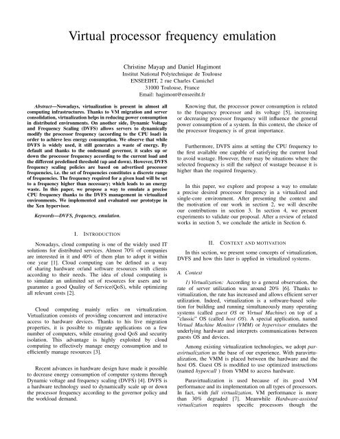
<strong>Virtual</strong> <strong>processor</strong> <strong>frequency</strong> <strong>emulation</strong><br />
Christine Mayap and Daniel Hagimont<br />
Institut National Polytechnique de Toulouse<br />
ENSEEIHT, 2 rue Charles Camichel<br />
31000 Toulouse, France<br />
Email: hagimont@enseeiht.fr<br />
Abstract—Nowadays, virtualization is present in almost all<br />
<strong>comp</strong>uting infrastructures. Thanks to VM migration and server<br />
consolidation, virtualization helps in reducing power consumption<br />
in distributed environments. On another side, Dynamic Voltage<br />
and Frequency Scaling (DVFS) allows servers to dynamically<br />
modify the <strong>processor</strong> <strong>frequency</strong> (according to the CPU load) in<br />
order to achieve less energy consumption. We observe that while<br />
DVFS is widely used, it still generates a waste of energy. By<br />
default and thanks to the ondemand governor, it scales up or<br />
down the <strong>processor</strong> <strong>frequency</strong> according to the current load and<br />
the different predefined threshold (up and down). However, DVFS<br />
<strong>frequency</strong> scaling policies are based on advertised <strong>processor</strong><br />
frequencies, i.e. the set of frequencies constitutes a discrete range<br />
of frequencies. The <strong>frequency</strong> required for a given load will be set<br />
to a <strong>frequency</strong> higher than necessary; which leads to an energy<br />
waste. In this paper, we propose a way to emulate a precise<br />
CPU <strong>frequency</strong> thanks to the DVFS management in virtualized<br />
environments. We implemented and evaluated our prototype in<br />
the Xen hypervisor.<br />
Keywords—DVFS, <strong>frequency</strong>, <strong>emulation</strong>.<br />
I. INTRODUCTION<br />
Nowadays, cloud <strong>comp</strong>uting is one of the widely used IT<br />
solutions for distributed services. Almost 70% of <strong>comp</strong>anies<br />
are interested in it and 40% of them plan to adopt it within<br />
one year [1]. Cloud <strong>comp</strong>uting can be defined as a way<br />
of sharing hardware or/and software resources with clients<br />
according to their needs. The idea of cloud <strong>comp</strong>uting is<br />
to simulate an unlimited set of resources for users and to<br />
guarantee a good Quality of Service(QoS), while optimizing<br />
all relevant costs [2].<br />
Cloud <strong>comp</strong>uting mainly relies on virtualization.<br />
<strong>Virtual</strong>ization consists of providing concurrent and interactive<br />
access to hardware devices. Thanks to his live migration<br />
properties, it is possible to migrate applications on a few<br />
number of <strong>comp</strong>uters, while ensuring good QoS and security<br />
isolation. This advantage is highly exploited by cloud<br />
<strong>comp</strong>uting to effectively manage energy consumption and to<br />
efficiently manage resources [3].<br />
Recent advances in hardware design have made it possible<br />
to decrease energy consumption of <strong>comp</strong>uter systems through<br />
Dynamic voltage and <strong>frequency</strong> scaling (DVFS) [4]. DVFS is<br />
a hardware technology used to dynamically scale up or down<br />
the <strong>processor</strong> <strong>frequency</strong> according to the governor policy and<br />
the workload demand.<br />
Knowing that, the <strong>processor</strong> power consumption is related<br />
to the <strong>frequency</strong> <strong>processor</strong> and its voltage [5], increasing<br />
or decreasing <strong>processor</strong> <strong>frequency</strong> will influence the general<br />
power consumption of a system. In this context, the choice of<br />
the <strong>processor</strong> <strong>frequency</strong> is of great importance.<br />
Furthermore, DVFS aims at setting the CPU <strong>frequency</strong> to<br />
the first available one capable of satisfying the current load<br />
to avoid wastage. However, there may be situations where the<br />
selected <strong>frequency</strong> is still the subject of wastage because it is<br />
higher than the required <strong>frequency</strong>.<br />
In this paper, we explore and propose a way to emulate<br />
a precise desired <strong>processor</strong> <strong>frequency</strong> in a virtualized and<br />
single-core environment. After presenting the context and<br />
the motivation of our work in section 2, we will describe<br />
our contributions in section 3. In section 4, we present<br />
experiments to validate our proposal. After a review of related<br />
works in section 5, we conclude the article in Section 6.<br />
II.<br />
CONTEXT AND MOTIVATION<br />
In this section, we present some concepts of virtualization,<br />
DVFS and how this later is applied in virtualized systems.<br />
A. Context<br />
1) <strong>Virtual</strong>ization: According to a general observation, the<br />
rate of server utilization was around 20% [6]. Thanks to<br />
virtualization, the rate has increased and allows efficient server<br />
utilization. Indeed, virtualization is a software-based solution<br />
for building and running simultaneously many operating<br />
systems (called guest OS or <strong>Virtual</strong> Machine) on top of a<br />
”classic” OS (called host OS). A special application, named<br />
<strong>Virtual</strong> Machine Monitor (VMM) or hypervisor emulates the<br />
underlying hardware and interprets communications between<br />
guests OS and devices.<br />
Among existing virtualization technologies, we adopt paravirtualization<br />
as the base of our experience. With paravirtualization,<br />
the VMM is placed between the hardware and the<br />
host OS. Guest OS is modified to use optimized instructions<br />
(named hypercall ) from VMM to access hardware.<br />
Paravirtualization is used because of its good VM<br />
performance and its implementation on all types of <strong>processor</strong>s.<br />
In fact, with full virtualization, VM performance is more<br />
than 30% degraded [7]. Meanwhile Hardware-assisted<br />
virtualization requires specific <strong>processor</strong>s though the
performance of guest OS are close-to-native performance.<br />
Paravirtualization is highly adopted and vulgarized by<br />
Xen [8] and VMWare ESX Server [9]. In this context, our<br />
work is based on Xen platform because it is prevalent in many<br />
<strong>comp</strong>uting infrastructures, as well as in the vast majority of<br />
our previous work.<br />
2) Dynamic Voltage and Frequency Scaling (DVFS): Today,<br />
all <strong>processor</strong>s integrate dynamic <strong>frequency</strong>/voltage scaling<br />
to adjust <strong>frequency</strong>/voltage during runtime. The decision to<br />
change the <strong>frequency</strong> is commanded by the current <strong>processor</strong>’s<br />
governor. Each governor has its own strategy to perform<br />
<strong>frequency</strong> scale. According to the configured policy, governor<br />
can decide to scale <strong>processor</strong> speed to a specific <strong>frequency</strong>,<br />
the highest, or the lowest <strong>frequency</strong>.<br />
Several governors are implemented inside the Linux kernel.<br />
Ondemand governor changes <strong>frequency</strong> depending on CPU<br />
utilization. It changes <strong>frequency</strong> from the lowest (whenever<br />
CPU utilization is less than a predefined (low therehold) to<br />
the highest and vice-versa. Performance governor always keeps<br />
the <strong>frequency</strong> at the highest value while slowest CPU speed<br />
is always set by powersave governor. Conservative governor<br />
decreases or increases <strong>frequency</strong> step-by-step through a range<br />
of <strong>frequency</strong> values supported by the hardware. Userspace<br />
governor allows user to manually set <strong>processor</strong> <strong>frequency</strong> [10].<br />
In order to control CPU <strong>frequency</strong>, governors use an underlying<br />
subsystem inside the kernel called cpufreqq [11].<br />
Cpufreq provides a set of modularized interfaces to allow<br />
changing CPU <strong>frequency</strong>. Cpufreq, in turn, relies on CPUspecific<br />
drivers to execute requests from governors.<br />
As aforementioned, effectively usage of DVFS brings the<br />
advantage of reducing power consumption by lowering <strong>processor</strong><br />
<strong>frequency</strong>. Moreover, almost all <strong>comp</strong>uting infrastructures<br />
possess multi-core and high <strong>frequency</strong> <strong>processor</strong>s. Thus, the<br />
benefit from using DVFS has been realized and achieved in<br />
many different systems.<br />
The next section describes the motivation of this work.<br />
B. Motivation<br />
During the last decade, several efforts have been made in<br />
order to find an efficient trade-off between energy consumption/resources<br />
management and applications performance.<br />
Most of them relies on DVFS, and are highly explored due<br />
to the advent of new modern powerful <strong>processor</strong>s integrating<br />
this technology.<br />
According to the ondemand governor (the default governor<br />
policy implemented by DVFS), the CPU <strong>frequency</strong> is<br />
dynamically changed depending on the CPU utilisation. With<br />
this governor, the highest available <strong>processor</strong> <strong>frequency</strong> is set<br />
when the CPU load is greater than a predefined threshold<br />
(up threshold). When the load decreases below the threshold,<br />
the <strong>processor</strong> <strong>frequency</strong> is decreased step by step until the one<br />
capable of satisfying the current process load is found.<br />
However, in most CPUs, the DVFS technology provides a<br />
reduced number of <strong>frequency</strong> levels (in the order of 5) [12].<br />
This configuration might not be enough for some experiments.<br />
Suppose a virtualized muti-core <strong>processor</strong> Intel(R)<br />
Xeon(R) E5520 with 2.261 GHz and the DVFS technology<br />
enable. Consider its six frequencies levels distributed as follows:<br />
1.596 GHz, 1.729 GHz, 1.862 Ghz, 1.995 Ghz, 2.128<br />
GHz and 2.261 GHz. Assume the host OS with a global load<br />
which needs 1.9285 Ghz to be satisfied. Knowing that the<br />
<strong>comp</strong>utation of the best execution time of an application is<br />
made on a basis of the maximum <strong>frequency</strong> of a <strong>processor</strong>,<br />
scheduling it with a lower <strong>frequency</strong> would end up with a<br />
lower than expected performance. From the SLA point of view<br />
and because of the non-existence of the expected <strong>frequency</strong>, the<br />
ondemand governor will set the CPU <strong>frequency</strong> to the first one,<br />
higher that the required <strong>frequency</strong>, capable of satisfying the<br />
current load. Precisely in our example, the ondemand governor<br />
will set the <strong>processor</strong> <strong>frequency</strong> to 1.995 GHz.<br />
However, it would be more beneficial in terms of energy to<br />
assign to the <strong>processor</strong> the exact required <strong>frequency</strong>. Indeed,<br />
the DVFS technology consists of concurrently lowering the<br />
CPU voltage and the CPU <strong>frequency</strong>. By lowering them, the<br />
current total energy consumption of the system is globally decreased<br />
[13]. To improve this well-known energy management,<br />
we will realise some adjustments on the DVFS technology.<br />
Hence, instead of setting the CPU <strong>frequency</strong> to the first higher<br />
available <strong>frequency</strong>, we decided to emulate some of the nonexistent<br />
CPU <strong>frequency</strong> according to the system needs.<br />
Concretely, emulating a CPU <strong>frequency</strong>, in our work, consists<br />
of executing the <strong>processor</strong> successively on the available<br />
frequencies around the desired CPU <strong>frequency</strong>. Our <strong>emulation</strong><br />
process is essentially based on the conventional operation of<br />
the DVFS. The use of the DVFS possesses as asset the fact of<br />
generating no overhead while switching between frequencies<br />
because it has been done in the hardware.<br />
The next section describes our contributions.<br />
III.<br />
CONTRIBUTION<br />
As previously mentioned, the main idea of this paper is<br />
to emulate a CPU <strong>processor</strong> <strong>frequency</strong> based on periodic<br />
oscillations of frequencies between two levels of successive<br />
frequencies. This extension will suggest a way of decreasing<br />
power consumption in virtualized systems while keeping good<br />
VM performance. The next section will expound our approach<br />
and the implementation we made.<br />
A. Our appraoch<br />
Our approach is two folds: (1) To determine the exact<br />
<strong>processor</strong> <strong>frequency</strong> need by the current load and (2) to<br />
emulate it if necessary.<br />
Let’s assume a host with several VMs running on it.<br />
Suppose that they generate a global load of W host . Consider<br />
that we need our CPU to be running at <strong>processor</strong> <strong>frequency</strong> of<br />
f host to satisfy the current load (W host ). However, the desired<br />
<strong>processor</strong> <strong>frequency</strong> f host is not present among the available<br />
<strong>processor</strong> frequencies of our host. This <strong>frequency</strong> need to be<br />
emulated.<br />
A weighted average can be defined as an average in which<br />
each quantity to be averaged is assigned a weight. These<br />
weightings determine the relative importance of each quantity<br />
on the average. Weightings are the equivalent of having that
many similar items with the same value involved in the<br />
average. Indeed, the <strong>emulation</strong> of CPU <strong>processor</strong> is based<br />
on weighted average of CPU <strong>frequency</strong> around the <strong>frequency</strong><br />
to emulate. Although it is possible to determine in advance<br />
the neighboring <strong>processor</strong> frequencies, the <strong>comp</strong>utation of the<br />
execution time for each of them is not realistic.<br />
Firstly, we need to determine the required <strong>frequency</strong> and<br />
later the both frequencies around the desired one. Assume that<br />
f high and f low are the <strong>frequency</strong> above and below the desired<br />
<strong>frequency</strong> respectively. To emulate f host , we need to <strong>comp</strong>ute<br />
our load during t high at f high and during t low at f low so that<br />
the required <strong>frequency</strong> f host is the weighted-average of f high<br />
with t high as weight and f low with t low as weight. It means<br />
that:<br />
f host = (f high × t high ) + (f low × t low )<br />
t high + t low<br />
(1)<br />
Unfortunately, it is not possible to determine beforehand<br />
the exact execution times allowing to fulfill the equation 1.<br />
Instead of considering t high and t low as the execution time, we<br />
exploited it as the occurrence count. Meaning that to emulate<br />
f host , the <strong>processor</strong> needs to be executed t high times in higher<br />
<strong>frequency</strong> f high and t low times in lower <strong>frequency</strong> f low .<br />
It is important to note that, the real execution time at<br />
each <strong>processor</strong> <strong>frequency</strong> level can be <strong>comp</strong>uted as follows:<br />
NumberOccur × T ickDuration . Where NumberOccur<br />
represents either t high or t low and T ickDuration the duration<br />
of each tick of reconfiguration.<br />
To validate this assumption, let’s consider the small example<br />
of II-B. By executing our <strong>processor</strong>, once on the lower<br />
<strong>frequency</strong> (that means at 1.862 Ghz) and once on the higher<br />
<strong>frequency</strong> (that means 1.995 Ghz), we will obtain the required<br />
<strong>frequency</strong> (1.9285 Ghz).<br />
It means that: f host = 1.995×1+1.862×1<br />
1+1<br />
= 1.9285<br />
As aforementioned, the number of executions at each<br />
<strong>processor</strong> <strong>frequency</strong> cannot be known at the beginning of the<br />
experiments. It must be dynamically <strong>comp</strong>uted.<br />
The next section presents our implementation.<br />
B. Implementation<br />
In this section, we address the design and the implementation<br />
choices of our <strong>frequency</strong> emulator, and the conditions of<br />
his exploitation.<br />
Our implementation is two folds: (1) checking the appropriate<br />
<strong>processor</strong> <strong>frequency</strong> for the current load and (2) emulating<br />
If it is not existing.<br />
1) Appropriate <strong>processor</strong> <strong>frequency</strong>: By default DVFS<br />
advertises a discrete range of <strong>processor</strong> frequencies. It means<br />
that, only a fixed and predefined number of <strong>processor</strong> frequencies<br />
are available.<br />
To fulfill the first aspect of our work (determine the<br />
adequate <strong>frequency</strong>), we assume that, on each <strong>processor</strong>, it<br />
is possible to have a continuous range of frequencies. Knowing<br />
that the difference between two successive frequencies<br />
is practically identical, we virtually subdivided them into 3<br />
(value obtained thanks to analysis and successive experiments).<br />
Indeed, this subdivision allowed the obtaining of the more<br />
moved closer frequencies. This nearness at the level of the<br />
frequencies so allowed to satisfy at best the <strong>processor</strong>’s loads.<br />
Assuming that the <strong>frequency</strong> range is now continuous, it is<br />
then always possible to have a precise <strong>processor</strong> <strong>frequency</strong> for<br />
a given load. The return of the suitable <strong>processor</strong> <strong>frequency</strong><br />
is made according to the <strong>frequency</strong> ratio presented in our<br />
proposal in [8].<br />
Indeed, at each tick of the scheduler, a monitoring module<br />
gathers the current CPU load of each VM. It then aggregates<br />
the total Absolute load of all the VM and <strong>comp</strong>utes the new<br />
<strong>processor</strong> <strong>frequency</strong> and the frequencies surrounding it, as<br />
depicted in the algorithm below (Listing 1) where<br />
• LFreq[]: represents a table of 3 <strong>processor</strong> frequencies<br />
classified as follows: the required <strong>frequency</strong> and the<br />
surrounding ones (higher and lower respectively)<br />
• VFreq: value obtained after the division of the interval<br />
between consecutive frequencies by 3. It is used to<br />
obtain some virtual <strong>processor</strong> frequencies.<br />
• Freq[]: represents the available <strong>processor</strong> frequencies.<br />
The table is sorted in descending order.<br />
We iterate on the <strong>processor</strong> frequencies (line 2). Following<br />
our assumption regarding frequencies (it will be validated in<br />
section IV-B1), we <strong>comp</strong>ute for each <strong>frequency</strong> the <strong>frequency</strong><br />
ratio (line 3) and check if the <strong>comp</strong>uting capacity of the<br />
<strong>processor</strong> at that <strong>frequency</strong> can absorb the current absolute<br />
load (line 6). If the current <strong>frequency</strong> can not satisfy the load,<br />
we iterate on virtual <strong>processor</strong> frequencies (line 22 to line 29).<br />
1 void <strong>comp</strong>uteNewFreq(int LFreq[], int VFreq) {<br />
2 for (i=1; i ratio){<br />
23 if (NFreq != Freq[i+1]){<br />
24 NFreq -= VFreq;<br />
25 ratio = NFreq/Freq[1];<br />
26 }<br />
27 else<br />
28 break;<br />
29 }<br />
30 if (ratio * 100 < Absolute_load){<br />
31 NFreq += VFreq;<br />
32 if (NFreq == Freq[i]){<br />
33 LFreq[1] = LFreq[2] = Freq[i];<br />
34 }<br />
35 LFreq[0] = NFreq;<br />
36 }<br />
37 }<br />
38 }<br />
Listing 1. Algorithm for <strong>comp</strong>uting the adequate <strong>processor</strong> <strong>frequency</strong> and<br />
the surrounding frequencies
By the end of the algorithm, if the required <strong>frequency</strong> is not<br />
among the known <strong>frequency</strong> of the <strong>processor</strong>, it is immediately<br />
emulated.<br />
2) Processor <strong>frequency</strong> <strong>emulation</strong>: The <strong>emulation</strong> is based<br />
on the cumulative functions principle. It is convenient to<br />
describe data flows by means of the cumulative function<br />
f(t), defined as the number of elements seen on the flow<br />
in time interval [0, t]. By convention, we take f(0) = 0,<br />
unless otherwise specified. Function f is always wide-sense<br />
increasing, it means that f(s) ≤ f(t) for all s ≤ t.<br />
Suppose 2 wide-sense increasing functions f and g, the<br />
notation f + g denotes the point-wise sum of functions f and<br />
g.<br />
(f + g)(t) = f(t) + g(t) (2)<br />
Notation f ≤ (=, ≥) g means that f(t) ≤ (=, ≥) g(t) for<br />
all t [14].<br />
To exploit this notion, we defined 3 cumulative <strong>frequency</strong><br />
functions: CumF high (t), CumF low (t) and CumF host (t).<br />
Where CumF high (t), CumF low (t) and CumF host (t) represent<br />
the functions for the higher <strong>processor</strong> <strong>frequency</strong> , the<br />
lower and the required <strong>processor</strong> <strong>frequency</strong> respectively. In<br />
our case, we defined the cumulative <strong>frequency</strong> corresponding<br />
to a particular value as the sum of all the frequencies up<br />
to and including that value. Meaning that: CumF high (t) =<br />
∑ t<br />
k=0 f high.<br />
At each tick of the scheduler and for each <strong>frequency</strong><br />
involved (including the emulated <strong>frequency</strong>) in the <strong>emulation</strong><br />
of the <strong>frequency</strong>, we <strong>comp</strong>ute its cumulative <strong>frequency</strong><br />
(Listing 2). The <strong>comp</strong>utation of each cumulative <strong>frequency</strong> is<br />
executed as follow:<br />
• Initially, the cumulative frequencies functions are<br />
equal to zero (their initial value). This value is reinitialized<br />
when the current load need a different <strong>frequency</strong><br />
or when the current one is already emulated<br />
(line 17),<br />
• At each tick, the cumulative <strong>frequency</strong> of the emulated<br />
<strong>frequency</strong> (CumF host (t)) is incremented by its value:<br />
CumF host (t) + = f host (line 7 and line13),<br />
• At each tick, only one <strong>frequency</strong> is set (either f high<br />
or f low ). The choice of the <strong>frequency</strong> is carried out as<br />
follows:<br />
◦ The sum of CumF high (t) and CumF low is<br />
<strong>comp</strong>uted according to the equation 2 and the<br />
result is <strong>comp</strong>ared to CumF host (t) (line 3),<br />
◦ If the sum is lower than CumF host (t), then<br />
the <strong>processor</strong> <strong>frequency</strong> is set to f high during<br />
the next quantum (line 6),<br />
◦ Else, if the sum is higher than CumF host , the<br />
<strong>processor</strong> <strong>frequency</strong> is set to f low during the<br />
next quantum (line 12),<br />
◦ If both are equal, the desired <strong>frequency</strong> was<br />
emulated and the different cumulative frequencies<br />
are reinitialized (line 17).<br />
Through these iterations and these oscillations, we managed<br />
to emulate our desired <strong>frequency</strong>. It should be mentioned that,<br />
the emulated <strong>frequency</strong> and the neighboring frequencies are<br />
obtained with the algorithm presented in Listing 1.These later<br />
(table LFreq[]) are passed as a parameter to the algorithm<br />
below.<br />
For instance, if we consider our example of section II-B,<br />
the goal was to emulate a <strong>processor</strong> <strong>frequency</strong> of 1.9285 Ghz.<br />
The surrounding frequencies are 1.995 Ghz and 1.862 Ghz.<br />
The execution of the algorithm of Listing 2 is as follows<br />
(Table I ):<br />
Init. CumFH = CumFL = CumF = SumFreq = 0<br />
cpuid = 0 ; NumbFH = NumFL = 0<br />
LFreq[0]=1.9285; LFreq[1]=1.995; LFreq[2]=1.862<br />
Step 1 SetFreq(0, LFreq[1]); CumFL = 0<br />
CumFH = 1.995 ; CumF = 1.9285<br />
NumbFH = 1;NumFL = 0 ; SumFreq= 1.995<br />
Step 2<br />
Step 3<br />
SumFreq ¿ CumF ⇒ SetFreq(0, LFreq[2]);<br />
CumFL = 1.862 ; NumFL = 1; CumFH = 1.995<br />
CumF = 3.857 ; NumbFH = 1, SumFreq = 3.857<br />
SumFreq = CumF ⇒ Init<br />
NumFL = 1 and NumFH = 1<br />
TABLE I.<br />
ALGORITHM VALIDATION<br />
This execution validates the number of time needed to<br />
emulate 1.9285 Ghz as presented in section III-A.<br />
1 void EmulateFrequency(int LFreq[], int CumFH,int CumFL,<br />
int CumF,int cpuid) {<br />
2 int SumFreq;<br />
3 SumFreq = CumFH + CumFL;<br />
4<br />
5 if (SumFreq < CumF){<br />
6 SetFreq(cpuid,LFreq[1]);<br />
7 CumF += LFreq[0];<br />
8 CumFH += LFreq[1];<br />
9 }<br />
10 else{<br />
11 if (SumFreq > CumF){<br />
12 SetFreq(cpuid,LFreq[2]);<br />
13 CumF += LFreq[0];<br />
14 CumFL += LFreq[2];<br />
15 }<br />
16 else{<br />
17 CumF = CumFH = CumFL = 0;<br />
18 }<br />
19 }<br />
20 }<br />
Listing 2.<br />
Emulate <strong>processor</strong> <strong>frequency</strong><br />
During this execution, we remind that there is a trigger<br />
in charge of the <strong>comp</strong>utation of the absolute load and the<br />
notification of the current desired <strong>frequency</strong>. This situation<br />
also leads to a reinitialization of all the cumulative frequencies<br />
value.<br />
The next section presents some experiments to validate our<br />
proposal.<br />
IV.<br />
VERIFICATION OF OUR PROPOSAL<br />
We previously presented our approach and its implementation<br />
in the default Xen credit scheduler. In this section, we will<br />
present the experiment environment, the application scenario<br />
and some experiments to validate our proposition.
A. Experiment environment and scenario<br />
Our experiments were performed on a DELL Optiplex 755,<br />
with an Intel Core 2 Duo 2.66GHz with 4G RAM. We run a<br />
Linux Debian Squeeze (with the 2.6.32.27 kernel) in a single<br />
<strong>processor</strong> mode. The Xen hypervisor (in his 4.1.2 version)<br />
is used as virtualization solution. The evaluation described<br />
below was performed with an application which <strong>comp</strong>utes an<br />
approximation of π. This application is called π-app. In this<br />
scenario, we aim at measuring an execution time.<br />
B. Verification<br />
1) Proportionality: In our validation, we rely on one main<br />
assumption: proportionality of <strong>frequency</strong> and performance.<br />
This property means that if we modify the <strong>frequency</strong> of the<br />
<strong>processor</strong>, the impact on performance is proportional to the<br />
change of the <strong>frequency</strong>.<br />
This proportionality is defined by:<br />
F i<br />
F max<br />
= T max<br />
T i<br />
(3)<br />
which means that if we decrease the <strong>frequency</strong> from<br />
F max down to F i , the execution time will proportionally<br />
increase from T max to T i . For instance, if F max is 3000 and<br />
F i is 1500, the <strong>frequency</strong> ratio is 0.5 which means that the<br />
<strong>processor</strong> is running 50% slower at F i <strong>comp</strong>ared to F max . So<br />
if we consider an application that runs in 10 mn at F max , the<br />
10<br />
same application will be <strong>comp</strong>leted at<br />
0.5 = 20mn at F i.<br />
To validate this proportionality rule, we conducted the<br />
following experiment. We ran different π-app workloads at<br />
different <strong>processor</strong> frequencies and measured the execution<br />
times, allowing us to verify the proportionality of <strong>frequency</strong><br />
ratios and execution time ratios. Figure 1 gives some of the<br />
results we obtained, which shows that <strong>frequency</strong> ratios and<br />
execution time ratios are very close, as assumed in equation 3.<br />
Fig. 1.<br />
Proportionality of <strong>frequency</strong> and execution time<br />
2) Validation: Our textbed advertises the following <strong>processor</strong><br />
<strong>frequency</strong>: 2.66GHz, 2.40GHz, 2.13GHz, 1,86GHz and<br />
1.60GHz.<br />
The first part of our validation consists on validate our<br />
approach of <strong>emulation</strong>. For this validation, we executed our π-<br />
app application initially at 2.4 Ghz. Based on our proposal, we<br />
will execute the same <strong>comp</strong>utation by emulating the <strong>frequency</strong><br />
2.4 Ghz. We started by a well-known <strong>frequency</strong> for this<br />
workshop, but others experiences not presented here emulate<br />
the non-existent <strong>frequency</strong>.<br />
Processour Frequency (MHz)<br />
Fig. 2.<br />
Processour Frequency (MHz)<br />
Fig. 3.<br />
2667<br />
2400<br />
2133<br />
1867<br />
1600<br />
2667<br />
2400<br />
2133<br />
1867<br />
1600<br />
10<br />
0<br />
0 100 200 300 400 500 0<br />
Execution of π-app at 2.4Ghz<br />
0<br />
Processor Frequency<br />
VM<br />
0<br />
0 100 200 300 400 500<br />
Emulation of 2.4Ghz with oscillations<br />
Processor Frequency<br />
VM<br />
According to figure 2, the execution time of the π-app<br />
is about 410 Units. While emulating the same <strong>processor</strong><br />
<strong>frequency</strong>, we obtained an execution time of 415 Units, as<br />
depicted by the figure 3. Based on this first use case, we can<br />
validate our approach. Furthermore, with similar experiences<br />
(not presented here), we have proved that the oscillation of the<br />
<strong>frequency</strong> in non intrusive.<br />
The second part consists of validating the <strong>emulation</strong> of<br />
a non-existent <strong>frequency</strong>. We executed our π-app application<br />
of the maximum <strong>frequency</strong> (figure 4 )and we recorded its<br />
execution time for future <strong>comp</strong>arisons (Cf. Table II ). Then,<br />
we choose two of our virtual <strong>processor</strong> frequencies (2.222<br />
Ghz and 2.576 GHz); we have emulated them to execute our<br />
application (respectively figure 5 and figure 6). Their execution<br />
time is used for <strong>comp</strong>arison with the expected execution<br />
time according to our proportionality rule (Cf. Table II). The<br />
expected time formula is: T i = Fmax×Tmax<br />
F i<br />
Thanks to this scenario, we can validate our implementation<br />
approach. After execution, we can conclude that the real<br />
execution time are almost equal to the expected time. Further<br />
evaluations are to be done in order to identify the possible<br />
weaknesses/advantages of this proposal.<br />
The next section presents the related works.<br />
100<br />
90<br />
80<br />
70<br />
60<br />
50<br />
40<br />
30<br />
20<br />
100<br />
90<br />
80<br />
70<br />
60<br />
50<br />
40<br />
30<br />
20<br />
10<br />
Load (%)<br />
Load (%)
Processor Frequency<br />
VM<br />
100<br />
Frequency Execution Expected time (s)<br />
(GHz) Time (s)<br />
Processour Frequency (MHz)<br />
2667<br />
2400<br />
2133<br />
1867<br />
1600<br />
90<br />
80<br />
70<br />
60<br />
50<br />
40<br />
Load (%)<br />
2.667 108.65<br />
2.222 131.52 T i = 2.667×108.65<br />
2.222 = 130.41<br />
2.578 112.79 T i = 2.667×108.65<br />
2.578 = 112.40<br />
TABLE II.<br />
EXECUTION TIME RESULTS<br />
30<br />
Fig. 4.<br />
Processour Frequency (MHz)<br />
Fig. 5.<br />
10<br />
0<br />
0 50 100 150 200 250 300 350 400 450 0<br />
2667<br />
2400<br />
2133<br />
1867<br />
1600<br />
Execution of π-app at maximum <strong>frequency</strong><br />
0<br />
Processor Frequency<br />
VM<br />
0<br />
0 100 200 300 400 500<br />
Execution of π-app at emulated <strong>frequency</strong> 2.22Ghz<br />
V. RELATED WORKS<br />
Numerous research projects have focused on optimization<br />
of the operating cost of data centers and/or cloud <strong>comp</strong>uters.<br />
Most of them concerned efficient power consumption [15].<br />
Proposed solutions are based on either virtualization or DVFS.<br />
In virtualized environment, power reduction is made possible<br />
through servers’ consolidation and live migration. Classic<br />
Processour Frequency (MHz)<br />
Fig. 6.<br />
2667<br />
2400<br />
2133<br />
1867<br />
1600<br />
0<br />
0<br />
0 50 100 150 200 250 300 350 400 450<br />
Execution of π-app at 2.578Ghz<br />
Processor Frequency<br />
VM<br />
20<br />
100<br />
90<br />
80<br />
70<br />
60<br />
50<br />
40<br />
30<br />
20<br />
10<br />
100<br />
90<br />
80<br />
70<br />
60<br />
50<br />
40<br />
30<br />
20<br />
10<br />
Load (%)<br />
Load (%)<br />
consolidation consists on gathered multiples VMs (according<br />
to their load) on top of a reduced number of physical <strong>comp</strong>uters<br />
[16].<br />
In [17], Verma et al. aims at minimizing power consumption<br />
using consolidation after server workload analysis. They<br />
design two new consolidation approaches based respectively<br />
on, peak cluster load and correlation between applications<br />
before consolidating. Mueen et al. Strategy for power reduction<br />
consists in categorizing servers in pools according to their<br />
workload and usage. After categorizing, server consolidation<br />
is executed on all categories based on their utilization ratio in<br />
the data center [18].<br />
As for the live migration, it consists of migrating a VM<br />
from a physical host to another without shutting down the<br />
VM. Korir et al [19] proposes a secure solution of power<br />
reduction based on live migration and server consolidation.<br />
Their security constraints are related to VM migration. Indeed,<br />
critical challenge of VM live migration appears when VM is<br />
still running when migration is in process. Well known attacks,<br />
such as Time-of-heck to time-of-use (TOCTTOU) [20] and<br />
replay attack, can be launched. In their solution, they design a<br />
live migration solution capable of avoiding VM to be exposed<br />
to eventual attacks.<br />
One of the most rising approaches in power reduction is<br />
Dynamic voltage and <strong>frequency</strong> scaling(DVFS) [21], where<br />
voltage/<strong>frequency</strong> can be dynamically modified according to<br />
the CPU load. In [22], the authors design a new scheduling<br />
algorithm to allocate VMs in a DVFS-enabled cluster by<br />
dynamically scaling the voltage. Precisely, Laszewski et al.<br />
minimizes the voltage of each <strong>processor</strong> of physical machine<br />
by scaling down their <strong>frequency</strong>. In addition, they schedule<br />
the VMs on those lower voltage <strong>processor</strong>s while avoiding to<br />
scale physical machine to high voltage.<br />
In general, those previous approaches only are focused<br />
on well-known <strong>processor</strong> <strong>frequency</strong>. In [12], Blucher et al.<br />
suggests some approaches of the CPU performance emulator.<br />
Precisely, they propose and evaluate three approaches named<br />
as : CPU-Hogs, Fracas and CPU-Gov. CPU-Hogs consists of a<br />
CPU-burner process which burn and degrades the initial CPU<br />
<strong>processor</strong> according to a predefined percentage. CPU-Hogs<br />
has the disadvantage of being responsible for deciding when<br />
CPUs will be available for user processes. With Fracas, every<br />
decision is made by the scheduler. With Fracas, one CPUintensive<br />
process is started on each core. Their scheduling<br />
priorities are then carefully defined so that they run for the<br />
desired fraction of time. CPU-Gov is a hardware based solution<br />
base. It consists on leveraging the hardware <strong>frequency</strong> scaling<br />
to provide <strong>emulation</strong> by switching between the two frequencies<br />
that are directly lower and higher than the requested emulate.
Although, those approaches are related to the CPU performance,<br />
they aim at emulating a predefined known <strong>processor</strong><br />
<strong>frequency</strong>. Concretely, their goal is the answer this question:<br />
Given a CPU (characterized by its CPU performance for<br />
example), how can we emulate another CPU with a precise<br />
characteristics? Their <strong>emulation</strong> is done once and experiments<br />
are executed on it. In our case, it consists of a realtime<br />
<strong>emulation</strong> of CPU and it constitutes a base for an energy<br />
aware resources management.<br />
VI.<br />
CONCLUSION AND PERSPECTIVES<br />
With the emergence of cloud <strong>comp</strong>uting environments,<br />
large scale hosting centers are being deployed and the energy<br />
consumption of such infrastructures has become a critical<br />
issue. In this context, two main orientations have been successfully<br />
followed for saving energy:<br />
• <strong>Virtual</strong>ization which allows to safely host several guest<br />
operating systems on the same physical machines<br />
and more importantly to migrate guest OS between<br />
machines, thus implementing server consolidation,<br />
• DVFS which allows adaptation of the <strong>processor</strong> <strong>frequency</strong><br />
according to the CPU load, thus reducing<br />
power usage.<br />
We observe that DVFS is mainly used, but still generates a<br />
waste of energy. In fact, the DVFS <strong>frequency</strong> scaling policies<br />
are based on advertised <strong>processor</strong> <strong>frequency</strong>. By default and<br />
thanks to the ondemand governor, it scales up or down the<br />
<strong>processor</strong> <strong>frequency</strong> according to the current load and the<br />
different predefined threshold (up and down). However, the<br />
set of <strong>frequency</strong> constitutes a discrete range of <strong>frequency</strong>. In<br />
this case, the <strong>frequency</strong> required for a specific load will almost<br />
be scaled to a <strong>frequency</strong> higher than expected; which leads to<br />
a non-efficient use of energy.<br />
In this paper, we proposed a technique which addresses this<br />
issue. With our approach, we are able to determine and allocate<br />
a more precise <strong>processor</strong> <strong>frequency</strong> according to the current<br />
load. We subdivided the interval between two frequencies of<br />
the <strong>processor</strong> into tinier virtual frequencies. This leads to<br />
simulate a continuous <strong>processor</strong> <strong>frequency</strong> range. With this<br />
configuration and the ratio proportionality rule, it is thus<br />
almost possible to set the suitable <strong>frequency</strong> for a given load.<br />
Furthermore, thanks to oscillations, made possible through the<br />
principle of cumulative <strong>frequency</strong>, between the frequencies<br />
surrounding the desired one, it was possible to emulate a nonexistent<br />
<strong>frequency</strong>.<br />
Our proposal was implemented in the Xen hypervisor<br />
running with its default Credit scheduler. Different scenarios<br />
were used to validate our assumptions and our proposal.<br />
Our main perspective is to sustain this proposal with a real<br />
world benchmark before a <strong>comp</strong>lete validation. Furthermore,<br />
we aim to investigate and address the issue of energy conserving<br />
while eventually exploiting this operation.<br />
VII.<br />
ACKNOWLEDGEMENT<br />
The work presented in this article benefited from the<br />
support of ANR (Agence Nationale de la Recherche) through<br />
the Ctrl-Green project.<br />
REFERENCES<br />
[1] Y. Ezaki and H. Matsumoto, “Integrated management of virtualized<br />
infrastructure that supports cloud <strong>comp</strong>uting: Serverview resource orchestrator,”<br />
Fujitsu Sci. Tech. J., vol. 47, no. 2, 2011.<br />
[2] A. J. Young, R. Henschel, J. T. Brown., G. von Laszewski, J. Qiu, and<br />
G. C. Fox, “Analysis of virtualization technologies for high performance<br />
<strong>comp</strong>uting environments,” in IEEE International Conference on Cloud<br />
Computing, 2011.<br />
[3] M. Armbrust, A. Fox, R. Griffith, A. D. Joseph, R. Katz, A. Konwinski,<br />
G. Lee, D. Patterson, A. Rabkin, I. Stoica, and M. Zaharia, “A view of<br />
cloud <strong>comp</strong>uting,” Communications of the ACM, vol. 53, no. 4, 2010.<br />
[4] M. Weiser, B. Welch, A. Demers, and S. Shenker, “Scheduling for<br />
reduced cpu energy,” in Proceedings of the 1st USENIX conference on<br />
Operating Systems Design and Implementation, 1994.<br />
[5] E. Seo, S. Park, J. Kim, and J. Lee, “Tsb: A dvs algorithm with quick<br />
response for general purpose operating systems,” Journal of Systems<br />
Architecture, vol. 54, no. 1-2, 2008.<br />
[6] D. Gmach, J. Rolia, L. Cherkasova, G. Belrose, T. Turicchi, and<br />
A. Kemper, “An integrated approach to resource pool management:<br />
Policies, efficiency and quality metrics,” in IEEE International Conference<br />
on Dependable Systems and Networks, 2008.<br />
[7] D. Marinescu and R. Krger, “State of the art in autonomic <strong>comp</strong>uting<br />
and virtualization,” 2007.<br />
[8] P. Barham, B. Dragovic, K. Fraser, S. Hand, T. Harris, A. Ho, R. Neugebauer,<br />
I. Pratt, and A. Warfield, “Xen and the art of virtualization,” in<br />
Proceedings of the nineteenth ACM symposium on Operating systems<br />
principles, 2003.<br />
[9] “Vmware esx web site.” [Online]. Available:<br />
http://www.vmware.com/products/vsphere/esxi-and-esx/index.html<br />
[10] D. Miyakawa and Y. Ishikawa, “Process oriented power management,”<br />
in International Symposium on Industrial Embedded Systems, 2007.<br />
[11] V. Pallipadi and A. Starikovskiy, “The ondemand governor: past, present<br />
and future,” in Proceedings of Linux Symposium, vol. 2, 2006.<br />
[12] T. Buchert, L. Nussbaum, and J. Gustedt, “Accurate <strong>emulation</strong> of CPU<br />
performance,” in 8th International Workshop on Algorithms, Models<br />
and Tools for Parallel Computing on Heterogeneous Platforms, 2010.<br />
[13] M. F. Dolz, J. C. Fernández, S. Iserte, R. Mayo, and E. S. Quintana-<br />
Ortí, “A simulator to assess energy saving strategies and policies in hpc<br />
workloads,” ACM SIGOPS Operating Systems Review, vol. 46, no. 2,<br />
2012.<br />
[14] J.-Y. L. Boudec and P. Thiran, Network calculus: a theory of deterministic<br />
queuing systems for the internet. LNCS 2050, Springer-Verlag,<br />
2001.<br />
[15] M. Poess and R. O. Nambiar, “Energy cost, the key challenge of<br />
today’s data centers: a power consumption analysis of tpc-c results,”<br />
Proceedings of the VLDB Endowment, vol. 1, no. 2, 2008.<br />
[16] W. Vogels, “Beyond server consolidation,” ACM Queue magazine,<br />
vol. 6, no. 1, 2008.<br />
[17] A. Verma, G. Dasgupta, T. K. Nayak, P. De, and R. Kothari, “Server<br />
workload analysis for power minimization using consolidation,” in<br />
Proceedings of the 2009 conference on USENIX Annual technical<br />
conference, 2009.<br />
[18] M. Uddin and A. A. Rahman, “Server consolidation: An approach to<br />
make data centers energy efficient and green,” International Journal of<br />
Scientific and Engineering Research, vol. 1, no. 1, 2010.<br />
[19] W. C. Sammy Korir, Shengbing Ren, “Energy efficient security preserving<br />
vm live migration in data centers for cloud <strong>comp</strong>uting,” International<br />
Journal of Computer Science Issues, vol. 9, no. 3, 2012.<br />
[20] M. Bishop and M. Dilger, “Checking for race conditions in file<br />
accesses,” in Computing Systems, vol. 2, 1996.<br />
[21] S. Lee and T. Sakurai, “Run-time voltage hopping for low-power realtime<br />
systems,” in Proceedings of the 37th Annual Design Automation<br />
Conference, 2000.<br />
[22] G. von Laszewski, L. Wang, A. Younge, and X. He, “Power-aware<br />
scheduling of virtual machines in dvfs-enabled clusters,” in IEEE<br />
International Conference on Cluster Computing, 2009.