SESSION GRAPH BASED AND TREE METHODS + RELATED ...

Int'l Conf. Foundations of Computer Science | FCS'12 | 1 

SESSION 

GRAPH BASED AND TREE METHODS + 

RELATED ISSUES 

Chair(s) 

TBA

2 Int'l Conf. Foundations of Computer Science | FCS'12 |


Algorithms for Finding Magic Labelings of Triangles 

James M. McQuillan 1 and Dan McQuillan 2 

1 School of Computer Sciences, Western Illinois University, Macomb, IL, USA 

2 Department of Mathematics, Norwich University, Northfield, Vermont, USA 

Abstract— We present a new algorithm for finding vertexmagic 

total labelings of disjoint unions of triangles. Since 

exaustive searches are infeasible for large graphs, we use a 

specialized algorithm designed to find labelings with very 

restrictive properties, and then attempt to generate other 

labelings from these. We show constructively that there exists 

a vertex-magic total labeling, VMTL, for each of the feasible 

values of 7C3, 9C3 and 11C3. 

Keywords: graph labeling, algorithm, vertex-magic 

1. Introduction 

Let G be a simple graph with vertex set V and edge set E. 

A total labeling of a graph is a bijective map f : V ∪ E −→ 

{1, 2, . . . , |V |+|E|}. The weight of a vertex v incident with 

edges e1, . . . , et is wtf (v) = f(v)+f(e1)+· · ·+f(et). The 

total labeling f is a vertex-magic total labeling, or VMTL, 

if the weight of each vertex is a constant. In this case, the 

constant is called the magic constant of the VMTL. If a 

graph G has a VMTL, then G is called a vertex-magic graph. 

Given a VMTL f of a graph G with degree ∆, there is a 

dual VMTL f ∗ of G in which f ∗ (x) = |V |+|E|+1−f(x) 

for each x ∈ V ∪ E. If the magic constant of f is h, then 

the magic constant of f ∗ is (∆ + 1)(|V | + |E| + 1) − h. 

The range of possible magic constants for a graph is called 

the spectrum of the graph. Assume that G is a 2-regular 

graph. Suppose further that G has a VMTL with magic 

constant h and with n = |V | = |E|. Then 

5n + 3 

2 

≤ h ≤ 

7n + 3 

. (1) 

2 

The integral values in this range are the feasible values for 

the 2-regular graph G. (See [24] and [34] for a more general 

discussion.) For a 2-regular graph, the dual of a VMTL with 

magic constant h is a VMTL with magic constant 6n+3−h. 

Problem 1.1: The VMTL problem: given a feasible magic 

constant h, does there exist a VMTL with magic constant 

h? 

There have been many exciting general VMTL constructions 

in recent years, such as [15], [11], and [22]. Some 

other important papers for labeling regular graphs include 

[21], [5], [13], [31], [2], [3] and [23]. For 2-regular graphs, 

Wallis proved in [33] that, for a vertex-magic regular graph 

G, the multiple graph sG is also vertex-magic provided that 

s is odd or the degree of G is odd. Gray gave VMTLs of 

C3 ∪ C2n, n ≥ 3 and C4 ∪ C2n−1, n ≥ 3 in [14]. In [27], it 

was shown that, for every s ≥ 4 even, sC3 is vertex-magic. 

For every s ≥ 6 even, sC3 has VMTLs with at least 2s − 2 

different magic constants. For every s odd, VMTLs for sC3 

with s + 1 different magic constants were also provided. In 

this paper, we are interested in algorithms that can be used 

to construct VMTLs in sC3. 

One approach to Problem 1.1 is to design an algorithm to 

construct VMTLs for certain special types of graphs. This 

is a part of our strategy as our algorithm is specifically 

designed for sC3. An algorithm could be designed in an efficient 

way using properties of those graph types. For example, 

in [4], algorithms were designed specifically for finding all 

VMTLs on cycles and wheels. They provide a table giving 

the total number of VMTLs on cycles C3 through C18. 

Moreover, they give the number of VMTLs for these for a 

given magic constant. They give a table giving the number of 

VMTLs for wheel graphs W3, . . . , W10. Moreover, they give 

the number of VMTLs for these for given magic constants. 

(They also give the number of VMTLs for some of the 

feasible magic constants for W11.) 

A second strategy for approaching this problem is to 

convert it into another well-studied problem. This approach 

is taken in [20], where they convert an instance of the 

VMTL problem into an instance of the satisfiability of 

boolean expressions problem. The SAT problem was the 

first NP-complete problem ([7]) and is fundamental to computer 

science. Variants of the Davis-Putnam algorithm ([9]), 

BDD’s ([6]), and BED’s ([1]) are the three main complete 

algorithms for the SAT problem. There are also many 

incomplete local search algorithms. GSAT, WalkSAT ([32]), 

and UnitWalk ([17]) were three of the early local search 

algorithms. There is a yearly competition to find an efficient 

SAT solver as part of the annual SAT conference [19]. Given 

the amount of research that has been done on this problem, 

it is natural to consider converting an instance of a problem 

into an instance of the SAT problem. 

A third strategy, which is the approach taken here, is 

to combine mathematical intuition for finding new VMTLs 

in certain graphs with very focused, specific algorithms to 

generate labelings with certain properties. With this strategy, 

labelings might be found that other more general algorithms 

could not find in a reasonable amount of time. Such labelings 

might then be used to construct other labelings. This strategy 

was used in [27] and [18]. 

As mentioned above, tables are provided in [4] that give 

the number of VMTLs for C3 through C18. (They note

4 Int'l Conf. Foundations of Computer Science | FCS'12 | 

that of those, C11 through C18 had not previously been 

enumerated.) For sC3, there appears to be fewer magic 

labelings than cycles of the same size. There are only 32 

non-isomorphic magic labelings in 3C3 ([27]) even though 

C9 has 1540 non-isomorphic magic labelings ([13]). This 

suggests that it will be difficult to write computer programs 

to generate VMTLs (in a reasonable amount of time) for 

sC3 when s is big. 

In the very important paper [16], a computer search was 

done in an attempt to find a VMTL with the biggest labels 

on the vertices (strong VMTL) for each 2-regular graph of 

order 7, 11, 13, 15. Based on their observations, they made 

the following conjecture: 

Conjecture 1.1 ([16] Conjecture 1): A 2-regular graph of 

odd order possesses a strong VMTL if and only if it is not 

of the form (2t − 1)C3 ∪ C4 or (2t)C3 ∪ C5. 

They also found by computer search, strong VMTLs for 

all 2-regular graphs of order 17 except C5 ∪4C3. It turns out 

that C5 ∪ 4C3 does possess a strong VMTL [18], disproving 

part of the conjecture. This suggests that 2-regular graphs 

with many triangles require special attention, and special 

algorithms for efficient computer searches. 

MacDougall’s conjecture states that every regular graph 

of degree at least 2 is vertex-magic except for 2C3. This 

remains an open problem. 

The rest of this paper is organized as follows. In Section 2, 

we explain the importance of common differences of components 

and as well as searching for specialized labelings in 

the design of efficient algorithms for solving Problem 1.1. In 

Section 3, we give a new algorithm for generating VMTLs 

for sC3. In Section 4, we answer Problem 1.1 in the 

affirmative for each feasible magic constant in each of 7C3, 

9C3 and 11C3. These three graphs have 21, 27 and 33 

vertices respectively; we give a VMTL for each feasible 

value for each of these graphs. 

2. The common difference of a component 

of sC3 

For the remainder of this paper, we restrict ourselves to 

the problem of finding VMTLs in sC3. 

Notation 2.1: Denote by [x1, x2, x3, x4, x5, x6] the labels 

of one component of sC3 written in the order vertex-edgevertex-edge-vertex-edge. 

(So, x1 is the vertex label of a 

vertex with weight x1 + x2 + x6.) 

Lemma 2.1 ([27] Lemma 2): Given a VMTL of sC3 with 

a component labeled [a1, b3, a2, b1, a3, b2], then b1 − a1 = 

b2 − a2 = b3 − a3. 

Consider a VMTL of sC3. Suppose that one of its 

components is labeled [a1, b3, a2, b1, a3, b2]. The common 

difference of this component is defined to be d = b1 − a1 = 

b2 − a2 = b3 − a3 ([27]). This concept is a key ingredient 

in our algorithm. Lemma 2.2 follows immediately from 

Lemma 2.1. We use it to make our algorithm more efficient. 

Lemma 2.2: Suppose that we have a VMTL of sC3 

with magic constant h, and that a component has common 

difference d and labels [a1, b3, a2, b1, a3, b2]. Then 

(i) bi = ai + d, i = 1, 2, 3; 

(ii) the weight of each vertex in that component is h = 

a1 + (a2 + d) + (a3 + d) = a1 + a2 + a3 + 2d; 

(iii) the vertex sum of that component is h − 2d; 

(iv) d = (h − (a1 + a2 + a3))/2; and 

(v) h − (a1 + a2 + a3) is an even integer. 

Proof: All of these follow immediately from Lemma 

2.1. 

While it is trivial to rearrange any of (ii)-(iv) to obtain 

the others in Lemma 2.2, we prefer to state all of (i)-(v) 

so that we can refer to them individually. In an algorithm, 

when presented with three integers as possible labels for the 

vertices of one component, we can remove that triple from 

any further consideration if h minus the sum of the three 

numbers is not even by Lemma 2.2 part (v). If we wanted a 

component to have a specific common difference, we could 

also remove a triple from contention for vertex labels of a 

component if any of a1 + d, a2 + d, a3 + d had already been 

assigned to other components by Lemma 2.2 part (i). We 

use techniques such as these in our algorithm. 

Because exhaustive computer searches are only feasible 

for small s, we chose to write computer programs that are 

specifically designed to look for VMTLs with very restrictive 

properties. Such a strategy might not lead to any examples 

of VMTLs, or perhaps it might lead to just a few sporadic 

examples. On the other hand, it might lead to some important 

examples that could be used to generate others. For example, 

consider the following special case of Problem 1.1. 

Problem 2.1: Given a feasible magic constant h of sC3, 

does there exist a VMTL with magic constant h such that 

the labels 1, 2, . . . , s0 are on vertices of different compents, 

s0 ≤ s, and such that the common difference on each of 

these s0 components is 3s? 

This seems like quite a restictive problem, but an efficient 

algorithm can be tailor-made for this problem, and any 

solution is very valuable when combined with the following 

lemma, as it could be used to generate many solutions to 

Problem 1.1, especially if s0 is close to s. 

Lemma 2.3 ([27] Lemma 3): Let s be a positive integer 

and let λ0 be a VMTL of sC3 with a magic constant of h. 

Assume that one of the components has a vertex labeled 1 

and a common difference of 3s. Then there exists another 

VMTL λ1 of sC3 with a magic constant of h − 3. 

We gave some solutions to Problem 2.1 in [27, Theorem 

4] for s odd, s0 = s, and [27, Theorem 6] for s ≥ 6 even, 

s0 = s − 2. 

3. A magic labeling algorithm for sC3. 

In this section, we present an algorithm for generating 

VMTLs in sC3. We will use the following proposition to 

make our algorithm more efficient.


Proposition 3.1: A VMTL of sC3 with a magic constant 

of h has sum of all vertex labels equal to 3s[2(6s + 1) − h]. 

Proof: Let SV denote the sum of all the vertex labels, 

and let SE denote the sum of all the edge labels. Let n = |V | 

and let m = |E|. It is easy to check that SV +SE = 1+2+ 

· · ·+(n+m) = (n+m)(n+m+1)/2 and SV +2SE = nh. 

(For proofs of these, see [27].) Here, n = m = 3s. Solving 

for SV yields the desired equality. 

In Algorithm 3.1 below, we assign labels to some components 

and then attempt to extend that to a VMTL. Our 

algorithm has a heavy emphasis on finding labels of vertices 

in individual components. We make sure that the appropriate 

and necessary edge labels are available at the same time. 

Here, we use Lemmas 2.1 and 2.2. If we know the vertex 

labels and the common differences of some components of 

a VMTL, we know the edge labels of those components. 

For convenience, we use the following term in this situation 

to refer to the labels assigned to some but not necessarily 

all of the components. An injective vertex magic labeling, 

IVML, of sC3 is an injective map f from a subset A of 

V ∪E into {1, 2, . . . , |V |+|E|} such that A consists of zero 

or more components of sC3, and the weight of each vertex 

in A is a constant. Given a VMTL, erasing the vertex and 

edge labels from one or more components gives an IVML. 

We are hoping to go in the other direction. We are hoping 

to extend some IVMLs to VMTLs. Note that Lemma 2.1 

applies to IVMLs as well as VMTLs. 

Algorithm 3.1: A VMTL algorithm for sC3: 

Input: 

(a) the value of s that you want to find VMTLs for. 

(b) if you are only interested in VMTLs for a particular 

magic constant h, then that value of h is taken as input 

as well. 

(c) any information about restrictions there are on any of 

the labels that can be used to make the program run 

faster. 

Output: all VMTLs that satisfy the given restrictions. 

Our algorithm uses the following procedures: 

1. main( ) 

If a particular value for the magic constant h was not 

given as input, then we can use a loop to look for 

VMTLs for all feasible values of h. Equation (1) gives 

the range of feasible values. If we denote by hmax and 

hmin the upper and lower bounds in this inequality 

respectively, then let hmid = ⌈(hmin +hmax)/2⌉. Then 

the loop could go from hmax down to hmid. By duality, 

the VMTLs for the other values of h can be generated 

later from those. (Note that the algorithm could look 

for VMTLs for different values of h in parallel.) 

For each value of h, calculate the sum k that the 

vertex labels of any VMTL must have according 

to Proposition 3.1. The main should then call the 

procedure whichLabelsAreF orV ertices by a call 

such as whichLabelsAreF orV ertices(s, h, {1, . . . , 

6s}, 3s, k, 0, 0, 0, null); described below. 

Note: Three of the arguments for this call are s, h and 

k. The argument {1, . . . , 6s} represents the set of all 

possible labels, and the argument 3s represents the size 

of a set of labels for the vertices. Other arguments are 

used for the recursive nature of that procedure. They 

are described in that procedure. 

2. procedure whichLabelsAreF orV ertices(int s, int h, 

int[ ] theNumbersF orLabels, int desiredSize, int 

desiredSum, int sizeSoF ar, int sumSoF ar, int 

currentIndexOfNumbersF orLabels, int[ ] soF ar- 

F orV ertices); 

This recursive procedure attempts to grow the empty 

set to sets each having size desiredSize and sum 

desiredSum. For each such set that is found, the 

procedure lookF orV MT LsUsingIt is called in the 

hope that it can be used to label the vertices of sC3 as 

part of VMTLs with magic constant h and vertex sum 

desiredSum. 

To grow the empty set to such a set of size desiredSize 

and sum desiredSum, we have parameters to keep 

track of the set of elements we have chosen so far, 

soF arF orV ertices (initially null), as well as its size, 

sizeSoF ar (initially 0), and its sum, sumSoF ar (initially 

0). The parameter currentIndexOfNumbers- 

F orLabels (initially 0) keeps track of what element of 

theNumbersF orLabels that we are currently considering 

to include from soF arF orV ertices. 

This recursive procedure could have multiple base 

cases. To make this procedure more efficient, one base 

case could simply return if 

length(theNumbersF orLabels) 

−currentIndexOfNumbersF orLabels 

< (desiredSize − sizeSoF ar). 

In such a case, there is no hope of extending so- 

F arF orV ertices to a desired set because there aren’t 

enough numbers left to consider in theNumbersF or- 

Labels to extend soF arF orV ertices to a set of size 

desiredSize. 

Another base case could simply return if sumSo- 

F ar > desiredSum, as there is no hope of extending 

soF arF orV ertices to a desired set because we’ve 

already exceeded the desired sum. 

Another base case could simply return if 

currentIndexOfNumbersF orLabels 

≥ length(theNumbersF orLabels) 

as we’ve reached the end of the elements being considered 

in numbersF orLabels in this case. 

This recursive procedure should have a base case corresponding 

to the successful generation of a set with the


properties mentioned. In this case it calls the procedure 

lookF orV MT LsUsingIt, 

lookF orV MT LsUsingIt(s, h, theNumbersF or- 

Labels, soF arF orV ertices); 

To complete this procedure, we need two recursive 

calls, one of which attempts to use the current element 

of theNumbersF orLabels to make a desired set of 

vertex labels, and the other of which attempts to make a 

desired set of vertex labels without the current element. 

The first corresponds to using the current element of 

theNumbersF orLabels, 

theNumbersF orLabels[currentIndexOfChoices]. 

We recurse with that together with the information in 

the parameter soF arF orV ertices for the last argument. 

(We also have to use the appropriate updated values 

for the sixth and seventh arguments corresponding 

to size and sum and the eighth argument corresponding 

to the element of theNumbersF orLabels that should 

be considered next.) 

The second recursive call corresponds to us not selecting 

the current element of theNumbersF orLabels. 

For this recursive call, no new information is being 

added to the information in soF arF orV ertices. 

The eighth argument corresponding to the element of 

theNumbersF orLabels needs to be updated. 

3. procedure lookF orV MT LsUsingIt(int s, int h, int[ ] 

theNumbersF orLabels, int[ ] theNumbersF orV ertices); 

Since we have a specific subset of all possible labels to 

use for the vertices, the remaining labels must be for 

the edges. Store these in int[ ] theNumbersF orEdges. 

Next, call the recursive procedure generateV MT Ls, 

with a call such as 

generateV MT Ls(theNumbersF orV ertices, the- 

NumbersF orEdges, h, s, {false, . . . , false}, null, 

−1); 

This procedure will attempt to generate VMTLs using 

these. 

4. procedure generateV MT Ls(int[ ] theNumbersF or- 

V ertices, int[ ] remainingNumbersF orEdges, int 

h, int s, boolean[ ] usedV ertexIndex, int[ ][ ] ivml- 

Indices, int[ ] commonDifferences, int currentIndex- 

OfIV ML); 

This procedure tries to find VMTLs by labeling one 

component at a time. The first parameter, theNumbersF 

orV erices, gives the set of numbers that is to 

be used for labeling all the vertices. The parameters 

ivmlIndices and commonDifferences keep track 

of an IVML that we are trying to grow. The parameter 

ivmlIndices keeps track of triples of indices 

in theNumbersF orV ertices. One triple corresponds 

to one component, so if we ever get s triples we 

have our vertex labels. From such a triple, the corre- 

sponding three elements in theNumbersF orV ertices 

are currently being used as the vertex labels for one 

component. The common difference for that component 

can be found in the appropriate element in 

commonDifferences. From these pieces of information, 

we have the edge labels for that component. 

As we grow an IVML, some labels are used for edges. 

The second parameter keeps track of the edge labels 

that have not as yet been used. The first parameter, 

theNumbersF orV ertices, is the set of all of the 

labels for the vertices, and the usedV ertexIndex 

parameter keeps track of those that have been used so 

far. 

This procedure has a base case corresponding to finding 

a solution. If the parameter ivmlIndices has length 

s, then it corresponds to a VMTL, in which case that 

information is outputted, and the procedure returns. 

This procedure has a loop to continually look for all 

possible labelings of one component that could be 

used to augment the information in ivmlIndices and 

commonDifferences, to give a bigger IVML. The 

corresponding edge labels need to be available. (Recall 

that Lemma 2.2 part (i) gives us these values.) If they 

are, then we can recurse on this bigger IVML with all 

parameters except the first updated. When the loop is 

finished, this procedure returns. 

It is important to note that we have several filters in 

place in the loop above so that (a) we ignore labels of 

a component that won’t lead to a solution, and (b) so 

that we ignore labels of a component that won’t lead 

to a specific type of solution that we are after. Filters 

of type (a) are used for the purposes of making the 

algorithm faster. If we exclude filters of the type (b), 

then our algorithm will find all possible VMTLs for the 

specified values of s and h. If we include filter of type 

(b), we will only be looking for VMTLs with certain 

properties. We often use filters of both types in order to 

find certain solutions quickly. We will discuss the use 

of filters further shortly. 

Finally, we can generate other VMTLs from the output of 

generateV MT Ls using Lemma 2.3. This can be done by 

hand (or by another procedure). 

Algorithm 3.1 uses several tools so that it is efficient: 

(i) In the main, our loop considered roughly half of the 

feasible magic constants. Duality can be used for the 

others. Parallelism can also be used here. 

(ii) In the second procedure, whichLabelsAreF orV ertices, 

we used the results of Proposition 3.1 to restrict 

the possibilities for sets of numbers to be considered as 

vertex labels. 

(iii) In generateV MT Ls( ), when we looked for a triple 

to label the vertices of one component, we eliminated 

possibilities that did not satisfy Lemma 2.2 part (v).


(iv) We were able to focus on labeling the vertices because 

of Lemma 2.2 part (iv). We just needed to make sure 

that the corresponding edge labels were available when 

we had labels that we liked for the vertices of a 

component. 

Sometimes, we are interested in finding only labellings 

in which some components have specific common differences. 

In this case, Lemma 2.2 part (iv) helps us 

reduce the number of triples that we need to consider 

as possible labels for the vertices of a component. In 

generateV MT Ls( ), when we looked for a triple to 

label the vertices of one component, we eliminated 

possibilities that did not satisfy Lemma 2.2 part (iv) 

in this situation. 

(v) Use Lemma 2.3 to generate many other VMTLs. 

In Algorithm 3.1, we use several filters. 

In generateV MT Ls, when we have an IVML with some 

components labeled, we try to extend it to VMTLs by 

labeling an additional component (recursively). Sometimes, 

a potential labeling of a “next” component can be removed 

from consideration (“filtered”) because we can tell that it 

will never lead to a VMTL, or because it will not lead to a 

specific type of VMTL that we are interested in finding. 

If we are given the common differences of any of the 

components as input, then some triples can be immediately 

eliminated from consideration as possible vertex labels for 

a component because of Lemma 2.2 part (iv). If restrictions 

are given, such as the common difference restiction of 

Problem 2.1, we might be able to eliminate triples here or 

at some other point in the algorithm. 

4. VMTLs for 7C3, 9C3, and 11C3. 

Using Algorithm 3.1, we now answer Problem 1.1 in 

the affirmative for 7C3, 9C3, and 11C3 for each of their 

respective feasible magic constants. In order to do so, we 

answer Problem 2.1 in the affirmative for certain values of 

h and s0 for 7C3, 9C3, and 11C3. Then, we use Lemma 2.3. 

Theorem 4.1: There exists VMTLs for all of the feasible 

values of 7C3. 

Proof: Consider the VMTL with components labeled 

[1, 37, 15, 22, 16, 36], [2, 39, 12, 23, 18, 33], 

[3, 42, 8, 24, 21, 29], [4, 40, 9, 25, 19, 30], 

[5, 38, 10, 26, 17, 31], [6, 41, 20, 13, 34, 27], 

and [7, 35, 11, 28, 14, 32]. 

This VMTL has a magic constant of 74. The first three 

components have common differences of 3s. Therefore, by 

using Lemma 2.3 three times, we have VMTLs of 7C3 with 

magic constants 71, 68, 65. By duality, there exist VMTLs 

with magic constants of 55, 58, 61 and 64. 

Next, consider the VMTL with components labeled 

[1, 37, 14, 22, 16, 35], [2, 38, 12, 23, 17, 33], 

[3, 42, 20, 11, 34, 28], [4, 40, 15, 18, 26, 29], 

[5, 36, 6, 31, 10, 32], [7, 39, 9, 25, 21, 27], 

and [8, 41, 13, 19, 30, 24]. 

This VMTL has a magic constant of 73. The first two components 

have common differences of 3s. By using Lemma 2.3 

twice, there exist VMTLs of 7C3 with magic constants 70 

and 67. By duality, there exist VMTLs with magic constants 

of 56, 59 and 62. 

Finally, in [27] it was shown that there exist VMTLs of 

7C3 with magic constants with values 75, 72, 69, 66, 63, 60, 

57, 54. 


values of 9C3. 


[1, 46, 18, 28, 19, 45], [2, 52, 11, 29, 25, 38], 

[3, 49, 13, 30, 22, 40], [4, 54, 12, 26, 32, 34], 

[5, 44, 9, 39, 10, 43], [6, 53, 16, 23, 36, 33], 

[7, 50, 27, 15, 42, 35], [8, 47, 31, 14, 41, 37], 

and [17, 51, 21, 20, 48, 24]. 



using Lemma 2.3 three times, we have VMTLs of 9C3 

with magic constants 89, 86, and 83. By duality, there exist 

VMTLs with magic constants of 73, 76, 79, and 82. 


[1, 47, 19, 28, 20, 46], [2, 50, 15, 29, 23, 42], 

[3, 51, 13, 30, 24, 40], [4, 49, 9, 36, 17, 41], 

[5, 52, 16, 26, 31, 37], [6, 45, 10, 39, 12, 43], 

[7, 53, 14, 27, 33, 34], [8, 54, 22, 18, 44, 32], 

and [11, 48, 25, 21, 38, 35]. 


components have common differences of 3s. By using 

Lemma 2.3 thrice, there exist VMTLs of 9C3 with magic 

constants of 91, 88 and 85. By duality, there exist VMTLs 

with magic constants of 71, 74, 77, and 80. 


[1, 50, 17, 28, 23, 44], [2, 47, 19, 29, 20, 46], 

[3, 51, 14, 30, 24, 41], [4, 54, 16, 25, 33, 37], 

[5, 48, 12, 35, 18, 42], [6, 53, 10, 32, 27, 36], 

[7, 45, 11, 39, 13, 43], [8, 49, 15, 31, 26, 38], 

and [9, 52, 22, 21, 40, 34]. 

This VMTL has a magic constant of 95. By duality, there 

exists a VMTL with a magic constant of 70. 


9C3 with magic constants with values 96, 93, 90, 87, 84, 81, 

78, 75, 72 and 69. 


values of 11C3.



[1, 62, 20, 34, 29, 53], [2, 65, 16, 35, 32, 49], 

[3, 61, 19, 36, 28, 52], [4, 57, 22, 37, 24, 55], 

[5, 60, 18, 38, 27, 51], [6, 56, 10, 50, 12, 54], 

[7, 66, 17, 33, 40, 43], [8, 63, 23, 30, 41, 45], 

[9, 59, 15, 42, 26, 48], [11, 58, 14, 44, 25, 47], 

and [13, 64, 21, 31, 46, 39]. 

This VMTL has a magic constant of 116. The first five 


using Lemma 2.3 five times, we have VMTLs of 119C3 with 

magic constants 113, 110, 107, 104 and 101. By duality, there 

exist VMTLs with magic constants of 85, 88, 91, 94, 97, and 

100. 


[1, 59, 22, 34, 26, 55], [2, 60, 20, 35, 27, 53], 

[3, 66, 13, 36, 33, 46], [4, 63, 15, 37, 30, 48], 

[5, 56, 10, 49, 12, 54], [6, 58, 17, 40, 24, 51], 

[7, 65, 19, 31, 41, 43], [8, 57, 11, 47, 18, 50], 

[9, 64, 23, 28, 45, 42], [14, 62, 21, 32, 44, 39], 

and [16, 61, 29, 25, 52, 38]. 

This VMTL has a magic constant of 115. The first four 

components have common differences of 3s. By using 

Lemma 2.3 four times, there exist VMTLs of 11C3 with 

magic constants of 112, 109, 106 and 103. By duality, there 

exist VMTLs with magic constants of 86, 89, 92, 95, and 98. 


11C3 with magic constants with values 117, 114, 111, 108, 

105, 102, 99, 96, 93, 90, 87 and 84. 

References 

[1] H.R. Andersen and H. Hulgaard, “Boolean Expression Diagrams,” 

Information and Computation, vol. 179, pp. 194-212, 2002. 

[2] M. Baca, M. Miller and J.A. MacDougall, “Vertex-magic total labelings 

of generalized Peterson graphs and convex polytopes,” J. Combin. 

Math. Combin. Comput., vol. 59, pp. 89-99, 2006. 

[3] M. Baca, M. Miller and Slamin, “Every generalized Peterson graph 

has a vertex-magic total labeling,” Int. J. Comp. Math., vol. 79, pp. 

1259-1263, 2002. 

[4] A. Baker and J. Sawada, “Magic Labelings on Cycles and Wheels,” 

in 2nd Annual International Conference on Combinatorial Optimization 

and Applications (COCOA ’08), Lecture Notes in Mathematics, 

vol. 5165, pp. 361-373, 2008. 

[5] O. Berkman, M. Parnas and Y. Roditty, “All cycles are edge-magic,” 

Ars Combin., vol. 59, pp. 145-151, 2001. 

[6] R.E. Bryant, “Symbolic Boolean Expression Manipulation with Ordered 

Binary Decision Diagrams,” ACM Computing Surveys, Vol. 24, 

No. 3, pp. 294-318, 1992. 

[7] S.A. Cook, “The complexity of theorem-proving procedures,” in 

Proceedings of the third annual ACM symposium on the Theory of 

computing, ACM, NY, 1971, pp. 151-158. 

[8] T.H. Cormen, C.E. Leiserson, R.L. Rivest, and C. Stein, Introduction 

to Algorithms, 3rd ed. MIT Press, 2009. 

[9] M. Davis, G. Logemann, and D. Loveland, “A Machine Program for 

Theorem Proving,” Communications of the ACM, vol. 3, pp. 394-397, 

1962. 

[10] G. Exoo, A.C.H. Ling, J.P. McSorley, N.C.K. Phillips, W.D. Wallis, 

“Totally magic graphs,” Discrete Math., vol. 254, pp. 103-113, 2002. 

[11] D. Froncek, P. Kovar and T. Kovarova, “Vertex magic total labeling 

of products of cycles,” Australas J. Combin., vol. 33, pp. 169-181, 

2005. 

[12] J.A. Gallian, “A dynamic survey of graph labeling,” Electronic J. 

Combin., vol. 17, #DS6, 2010. 

[13] R.D. Godbold and P.J. Slater, “All cycles are edge-magic,” Bull. Inst. 

Combin. Appl., vol. 22, pp. 93-97, 1998. 

[14] I. Gray, “New construction methods for vertex-magic total labelings 

of graphs,” Ph.D. thesis, University of Newcastle, 2006. 

[15] I. Gray, “Vertex-magic total labellings of regular graphs,” SIAM J. 

Discrete Math., vol. 21, Issue 1, pp. 170-177, 2007. 

[16] I.D. Gray and J.A. MacDougall, “Vertex-magic labelings of regular 

graphs II.,” Discrete Math., vol. 309, pp. 5986-5999, 2009. 

[17] E.A. Hirsch, and A. Kojevnikov, “UnitWalk: A new SAT solver 

that uses local search guided by unit clause elimination,” Annals of 

Mathematics and Artificial Intelligence, vol. 43, pp. 91-111, 2005. 

[18] J. Holden, D. McQuillan, and J.M. McQuillan, “A conjecture on strong 

magic labelings of 2-regular graphs,” Discrete Mathematics, vol. 309, 

pp. 4130-4136, 2009. 

[19] The International Conferences on Theory and Applications of Satisfiability 

Testing (SAT). [Online]. Available: http://www.satisfiability.org 

[20] G. Jäger, “An effective SAT encoding for magic labeling,” in Proceedings 

of the 9th Cologne Twente Workshop on Graphs and Combinatorial 

Optimization (CTW 2010), 2010, pp. 97-100. 

[21] A. Kotzig and A. Rosa, “Magic valuations of finite graphs,” Canad. 

Math. Bull., vol. 13, pp. 451-461, 1970. 

[22] P. Kovar, “Vertex magic total labeling of products of regular VMT 

graphs and regular supermagic graphs,” J. Combin. Math. Combin. 

Comput., vol. 54, pp. 21-31, 2005. 

[23] Y. Lin and M. Miller, “Vertex-magic total labelings of complete 

graphs,” Bull. Inst. Combin. Appl., vol. 33, pp. 68-76, 2001. 

[24] J.A. MacDougall, M. Miller, Slamin, and W.D. Wallis, “Vertex-magic 

total labelings of graphs,” Utilitas Mathematica, vol. 61, pp. 3-21, 

2002. 

[25] D. McQuillan, “Edge-magic and vertex-magic total labelings of certain 

cycles,” Ars Combin., vol. 91, pp. 257-266, 2009. 

[26] D. McQuillan, “A technique for constructing magic labelings of 

2−regular graphs,” JCMCC, vol. 75, pp. 129-135, 2010. 

[27] D. McQuillan and J.M. McQuillan, “Magic Labelings of Triangles,” 

Discrete Mathematics, vol. 309, pp. 2755-2762, 2009. 

[28] D. McQuillan and K. Smith, “Vertex-magic total labeling of multiple 

complete graphs,” Congr. Numer., vol. 180, pp. 201-205, 2006. 

[29] D. McQuillan and K. Smith, “Vertex-magic total labeling of odd 

complete graphs,” Discrete Math., vol. 305, pp. 240-249, 2005. 

[30] J.P. McSorley and W.D. Wallis, “On the spectra of totally magic 

labelings,” Bull. Inst. Combin. Appl., vol. 37, pp. 58-62, 2003. 

[31] Y. Roditty and T. Bachar, “A note on edge-magic cycles,” Bull. Inst. 

Combin. Appl. vol. 29, pp. 94-96, 2000. 

[32] B. Selman, H. Kautz, and B. Cohen, “Local Search Strategies for 

Satisfiability Testing,” in Cliques, Coloring, and Satisfiability: Second 

DIMACS Implementation Challenge, October 11-13, 1993. 

[33] W.D. Wallis, “Vertex magic labelings of multiple graphs,” Congr. 

Numer., vol. 152, pp. 81-83, 2001. 

[34] W.D. Wallis, Magic Graphs. Boston, MA: Birkhauser, 2001. 

[35] W.D. Wallis, “Two results of Kotzig on magic labelings,” Bull. Inst. 

Combin. Appl., vol. 36, pp. 23-28, 2002.


Assortativity of links in directed networks 

Mahendra Piraveenan 1 , Kon Shing Kenneth Chung 1 , and Shahadat Uddin 1 

1 Centre for Complex Systems Research, Faculty of Engineering and IT, 

The University of Sydney, NSW 2006, Australia 

Abstract— Assortativity is the tendency in networks where 

nodes connect with other nodes similar to themselves. Degree 

assortativity can be quantified as a Pearson correlation. 

However, it is insufficient to explain assortative or disassortative 

tendencies of individual links, which may be contrary 

to the overall tendency in the network. In this paper we 

define and analyse link assortativity in the context of directed 

networks. Using synthesised and real world networks, we 

show that the overall assortativity of a network may be due 

to the number of assortative or disassortative links it has, 

the strength of such links, or a combination of both factors, 

which may be reinforcing or opposing each other. We also 

show that in some directed networks, link assortativity can 

be used to highlight subnetworks which have vastly different 

topological structures. The quantity we propose is limited 

to directed networks and complements the earlier proposed 

metric of node assortativity. 

Keywords: Complex networks, graph theory, assortativity, social 

networks, biological networks 


In the last few decades, network approaches have been 

widely used to analyze complex systems in a number of 

domains, including technical, biological, social and physical 

domains [1], [2]. Assortativity is a much studied concept in 

the topological analysis of complex networks [3], [4], [5], 

[6]. Assortativity has been defined to quantify the tendency 

in networks where individual nodes connect with other nodes 

which are similar to themselves [3]. Thus, a social network 

of people tends to be assortative, since people often prefer to 

be friends with, or have links to, other people who are like 

them. A food web could be argued as disassortative, because 

predator and prey are unlikely to be similar in many respects. 

However, it is clear that the assortativity of a network needs 

to be defined in terms of a particular attribute of nodes in 

that network. A social network could be assortative when 

the considered attribute is the age of people, because people 

tend to be friends with other people similar to their age: 

however, the same network could be disassortative, when 

the gender of individuals is the considered attribute. Degree 

assortativity is the most common form of assortativity used 

in network analysis, whereby similarity between nodes is 

defined in terms of the number of connections the nodes 

have. Degree assortativity can be defined and quantified 

as a Pearson correlation [3], [7]. It has been shown that 

many technological and biological networks are slightly 

disassortative, while most social networks, predictably, tend 

to be assortative in terms of degrees [3], [5]. Recent work 

defined degree assortativity for directed networks in terms 

of in-degrees and out-degrees, and showed that an ensemble 

of definitions are possible in this case [6], [7]. 

It could be argued, however, that the overall assortativity 

tendency of a network may not be reflected by individual 

links of the network. For example, it is possible that in a 

social network, which is overall assortative, some people 

may maintain their ‘fan-clubs’. In this situation, people who 

have a great number of friends may be connected to people 

who are less famous, or even loners. If there is a link which 

connects such a popular person with a loner, that link cannot 

be called an assortative link, even though the network is 

overall assortative. Similarly, in a network which is overall 

disassortative many links could arguably be assortative. A 

good example for this is the so-called rich club scenario 

in internet AS networks [8]. Even though these networks 

display overall disassortativity, it has been shown that the 

hubs among them are strongly connected to each other, 

forming a ‘rich-club’. The links that connect these hubs, 

therefore should be considered assortative in nature. These 

examples highlight that the ‘local assortativity’ of links is a 

quantity, which, if defined, can throw light on the topological 

structure of networks. In directed networks, this can be 

defined separately for out-degree based mixing patterns and 

in-degree based mixing patterns. 

Indeed, decomposing the assortativity coefficient of a 

network into values for network components has already 

been attempted, and the metric of ‘local assortativity’ has 

been defined and analysed in detail [4], [6]. However, this 

decomposition has been done in terms of network nodes, 

rather than network links. In this work however, we propose 

to analyze the ‘local assortativity’ of individual links, and 

will demonstrate that this approach has its advantages, 

particularly for defining the assortativity of sub networks 

or regions. We limit our analysis to directed networks. 

Analyzing the ‘local assortativity’ of links can give us 

a number of insights about networks. We will be able to 

identify ‘positive’ and ‘negative’ links in the network in 

terms of assortativity, and based on these we can see which 

links help, or hinder, the overall assortative tendency in 

networks. We can identify if assortativity of a network is 

primarily determined by the number of a particular type 

of links, or rather by the strength of such links. If the


‘strength’ of a minority of links is the primary reason for 

a network’s assortativity, then we could predict that, if the 

network evolves, its assortativity may change rapidly. Link 

assortativity can be an indicator of the importance of links in 

the network, particularly if the links are highly assortative. 

Furthermore, profiles of link assortativity will provide us 

with yet another tool to classify networks. 

Our paper is structured as follows: in the next section, 

we will introduce the concept of link assortativity for directed 

networks. We will use the definition of assortativity 

described in [7] to establish this concept, since this form of 

definition is most conducive for link-based decomposition. 

Then we will analyze the link-based assortativity profiles of 

a number of synthesized and real world directed networks. 

These include citation networks, Gene regulatory networks, 

transcription networks, foodwebs and neural networks. We 

will draw observations from this analysis, showing that a 

network could be either assortative, disassortative or nonassortative, 

due to a number of combinations between the 

ratio of ‘positive’ and ‘negative’ links, and the average 

strength of such links. We will also look at link-assortativity 

distributions of a number of networks, and discuss what 

insights can be gained from these about the evolution and 

functionality of these networks. Finally we will present our 

summary and conclusions. 

2. Link assortativity of directed networks 

Degree assortativity has been defined by Newman, as a 

Pearson correlation between the ‘expected degree’ distribution 

qk, and the ‘joint degree’ distribution ej,k [3]. The 

expected degree distribution is the probability distribution of 

traversing the links of the network, and finding nodes with 

degree k at the end of the links. Similarly, the ‘joint degree’ 

distribution is the probability distribution of an link having 

degree j on one end and degree k on the other end. In the 

undirected case, the normalized Pearson coefficient of ej,k 

and qk gives us the assortativity coefficient of the network, 

r. 

If a network has perfect assortativity (r = 1), then all 

nodes connect only with nodes with the same degree. For 

example, the joint distribution ej,k = qkδj,k where δj,k is 

the Kronecker delta function, produces a perfectly assortative 

network. If the network has no assortativity (r = 0), then any 

node can randomly connect to any other node. A sufficiency 

condition for a non-assortative network is ej,k = qjqk. If 

a network is perfectly disassortative (r = −1), all nodes 

will have to connect to nodes with different degrees. A star 

network is an example of a perfectly disassortative network, 

and complex networks with star ‘motifs’ in them tend to be 

disassortative. 

In the case of directed networks, the definition is a 

bit more involved due to the existence of in-degrees and 

out-degrees. Therefore, we must consider the probability 

distribution of links going out of source nodes with j out- 

degrees, denoted as q out 

j , and the probability distribution of 

links going into target nodes with k in-degrees, denoted q in 

k . 

In addition, we may consider the probability distribution of 

links going into target nodes with k out-degrees, denoted 

˘q out 

k , and the probability distribution of links going out of 

source nodes with j in-degrees, denoted ˘q in 

j . In general, 

qout k ̸= ˘q out 

k and qin j ̸= ˘q in 

j [6]. 

We can also consider distribution e out,out 

j,k , abbreviated as 

eout j,k , as the joint probability distribution of links going into 

target nodes with k out-degrees, and out of source nodes of 

j out-degrees (i.e., the joint distribution in terms of outdegrees). 

Similarly, ein j,k = ein,in 

j,k is the joint probability 

distribution of links going into target nodes of k in-degrees, 

and out of source nodes of j in-degrees (i.e., the joint 

distribution of in-degrees). 

we can therefore define the out-assortativity of directed 

networks, as the tendency of nodes with similar out-degrees 

to connect to each other. Using the above distributions, outassortativity 

is formally defined, for out-degrees j and k, by 

Piraveenan et al [6] as 

rout = 

1 

σout q σout ⎡⎛ 

⎣⎝ 

˘q 

∑ 

jke out 

⎞ 

⎠ 

j,k − µ out 

jk 

q µ out 

˘q 

⎤ 

⎦ (1) 

where µ out 

q is the mean of qout k , µ˘q is the mean of ˘q out 

k , σout q 

is the standard deviation of qout k , and σout 

˘q is the standard 

deviation of ˘q out 

k . 

Similarly, Piraveenan et al. [6] defined in-assortativity as 

the tendency in a network for nodes with similar in-degrees 

to connect to each other, and this was formally specified as: 

1 

rin = 

σin q σin ⎡⎛ 

⎣⎝ 

˘q 

∑ 

jke in 

⎞ 

⎠ 

j,k − µ in 

q µ in 

⎤ 

⎦ 

˘q (2) 

jk 

where µ in 

q is the mean of qin k , µin 

˘q is the mean of ˘q in 

k , σin q is 

the standard deviation of qin k , σin 

˘q is the standard deviation 

of ˘q in 

k . 

Meanwhile, Foster et al. [7] also defined assortativity of 

directed networks in terms of the above distributions. While 

they used a different set of notations, using our notation their 

definition for out-assortativity can be written as 

rout = 

M −1 

σ out 

q σ out 

˘q 

[ ∑ 

i 

(j out 

i 

− µ out 

q )(k out 

i − µ out 

˘q ) 

where M is the number of links. Similarly, the definition of 

Foster et al. for in-assortativity can be written as 

[ 

−1 M ∑ 

rin = (j in 

i − µ in 

q )(k in 

i − µ in 

] 

˘q ) (4) 

σ in 

q σ in 

˘q 

i 

] 

(3)


It can be analytically proven that the definitions of Foster 

et al. for out-assortativity and in-assortativity are equivalent 

to the definitions of Piraveenan et al. for the same quantities 

respectively. That is, R.H.S of Eq. 1 = R.H.S of Eq. 3 and 

R.H.S of Eq. 2 = R.H.S of Eq. 4. Such a proof is given 

in our recent work [9] and it is beyond the scope of this 

paper to repeat it here. However, the key difference of the 

equivalent definitions is in the way the sums are obtained. 

While in the definitions of Piraveenan et al. the summations 

are obtained by traversing over degrees, in Foster et al. the 

summations are obtained by traversing over links. 

Indeed, from Eq. 3 it is apparent that the out-assortativity 

of a network can be decomposed into individual contributions 

of links in that network. the summation of the contribution, 

in turn, gives the overall network out-assortativity. 

Therefore, we can write that 

where ρ out 

e 

rout = ∑ 

i 

ρ out 

e 

is the individual contribution of a given link i to 

the out-assortativity of the network, and is given by 

ρ out 

e = 

M −1 

σ out 

q σ out 

˘q 

[ (j out 

i 

− µ out 

q )(k out 

i − µ out 

˘q ) ] 

Similarly, the contribution of an individual link to the 

overall in-assortativity of a network is given by 

ρ in 

e = 

M −1 

σ in 

q σ in 

˘q 

The definitions ρ out 

e 

[ (j in 

i − µ in 

q )(k in 

i − µ in 

˘q ) ] 

(5) 

(6) 

(7) 

and ρ in 

e indicate that, individual links 

can be classified as ‘assortative’ or ‘disassortative’ in the 

context of out-degree and in-degree mixing respectively, by 

considering the sign of these quantities. 

We also observe that in most networks, there will be a 

correlation between the sign of link assortativity of a link, 

and the degrees of nodes it connects. Intuitively, a link 

that connects a smaller-degreed node with a larger-degreed 

node will be disassortative, while an link which connects 

two similar degreed nodes will be assortative. We found 

evidence of this in both synthetic and real world networks. 

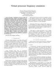
For example, in Fig. 1 we show the average link-assortativity 

against the differences in degrees at either end of links, for 

a simulated Erdos - Renyi random network. On the x-axis is 

shown the absolute difference between degrees of two nodes 

that are at the ends of an link. On y-axis, we calculate and 

show the average of link assortativity values for all links 

that have such a degree-difference. The figure clearly shows 

that, as the difference between the degrees increase, the 

links become more and more disassortative, as expected. We 

obtained similar results for a range of simulated scale-free 

networks. 

Fig. 2 demonstrates the same concept in a different 

manner. In this figure, the sum of degrees at either end of 

an link are shown, rather than the difference. If the sum is 

very high, it means that both ends of a link have high-valued 

degrees, where as if the sum is low, it means that both ends 

of a link have low-valued degrees. In both cases, we see 

that, on average, the links are assortative. If the sum is in 

the middle ranges however, it typically may mean that one 

end of the link has a high degree and the other end has a 

lower degree. Only a minority of links will have exactly the 

same middle-valued degrees on both ends. Here, predictably, 

most links are disassortative. 

avgerage link assortativity 

0.0002 

0 

-0.0002 

-0.0004 

-0.0006 

-0.0008 

-0.001 

2 4 6 8 10 12 14 

difference of degrees of links 

Fig. 1: Average link assortativity vs degree. The x-axis shows 

the difference between degrees at either end for a given 

link. The y-axis shows the average link assortativity of all 

links corresponding to the given x-value. As the difference 

between degrees increases, links on average become more 

disassortative. 

average link assortativity 

0.0012 

0.001 

0.0008 

0.0006 

0.0004 

0.0002 

0 

-0.0002 

5 10 15 20 25 

sum of degrees of links 

Fig. 2: Average link assortativity vs degree. The x-axis 

shows the sum of degrees at either end for a given link. 

The y-axis shows the average link assortativity of all links 

corresponding to the given x-value. It could be seen that, as 

the sum of degrees increases, links on average first become 

more disassortative and then more assortative.


3. Link assortativity of real world networks 

We analyzed link assortativity patterns of a number of 

real world networks, including Gene regulatory networks, 

transcription networks, cortical networks, neural networks, 

food webs, and citation networks. An explanation is necessary 

to some of these types of networks, since the usage 

of names can be ambiguous. In our transcription networks, 

nodes are regulatory genes and regulated proteins, and the 

links are the interactions between them [1]. These are 

bipartite and directed networks. On the other hand, by gene 

regulatory networks we mean networks where nodes are 

genes, and the links are the inhibitory or inducing effects of 

one gene on the expression of another gene [10]. Note the 

subtlety that unlike transcription networks, only genes are 

considered as nodes in these directed networks. Similarly, by 

cortical networks we denote the networks of dependencies 

between various regions of the cerebral cortical (in a set of 

primates)[11]. The nodes are regions in the cortical, and the 

links are functional dependencies. Note that the nodes are 

not individual neurons. On the other hand, neural networks 

are networks where nodes are individual neurons belonging 

to an organism’s neural system and links are anatomical connections 

between neurons [1]. In citation networks, nodes are 

research papers (or other citable documents) and links denote 

citations between these documents. In food webs, nodes are 

organisms in an ecosystem and the links represent predatorprey 

relationships between them [5]. These networks can 

be considered undirected or directed (prey to predator). A 

list of real world networks that we have studied is shown in 

Table 1, along with their out-assortativity and in-assortativity 

values. This is the same set studied in [6]. 

Table 2 shows the number of assortative and disassortative 

links in each network ( Mal and Mdl), as well as the 

average strength of assortative and disassortative links in 

these networks ( < S >al and < S >dl). The average 

strength is calculated by summing the local link assortativity 

values of all links which are assortative or disassortative, 

and dividing it by their count. This is done for both outassortativity 

and in-assortativity. It is apparent from the 

table that the assortativity coefficient of a network can be 

determined by (a) the numerical superiority of one type of 

links over the other (b) the strength superiority, on average, 

of one type of links over the other (c) a combination of these 

two factors, mutually reinforcing or otherwise. Specifically, 

we can observe the following scenarios. 

In terms of out-assortatativity: 

1) A Network can be assortative because a) it has more 

assortative links than disassortative links [such as C. 

elegans neural network, Human GRN, Chesapeake 

lower foodweb, E. coli and C. glutamicum transcription, 

Sci met, small World and Zewail citation networks, 

and human cortical] ) The assortative links are, 

on average, stronger than disassortative links [No real 

world example] c) a combination of these two reasons 

[The GRNs of C. elegans, A. thaliana, R. norvegicus 

and M. musculus] 

2) A network can be disassortative because a) it has more 

disassortative links than assortative links [transcription 

networks of C. jeikeium and C. efficiens] b) disassortative 

links are, on average, stronger than assortative 

links [No real world example] c) a combination of 

these two reasons [no real world example] 

3) A network can be nearly non-assortative because a) 

It has almost equal assortative and disassortative links 

with equal strength on average [The food webs of Bay 

dry, chrystal D, chrystal C, Chessapeake upper, Bay 

wet, and the cortical networks of cat and macaque] b) 

It has more assortative links, but disassortative links 

are on average stronger [Lederburg, self organizing 

maps, and smart Grid citation networks] c) It has more 

disassortative links, but assortative links are on average 

stronger [No real world example] 

The statement ‘no real world example’ is of course 

limited to the directed networks we have studied. As more 

directed networks are analysed, it is our hope that real world 

examples will turn up to illustrate the relevant scenarios. 

A number of interesting contrasts can be made from 

these observations. For example, most foodwebs are nonassortative 

simply because there are equal number of assortative 

and disassortative links, with equal strength on 

average. However, many citation networks are also nearly 

non-assortative, for a very different reason. They all have 

more assortative links, but their disassortative links are 

much stronger! For example, the Lederburg citation network 

has 26730 assortative links to 14872 disassortative links, 

but its disassortative links are almost doubly stronger on 

average, making it overall rather non-assortative (r = 0.06). 

Similarly, while most assortative networks are assortative 

simply because they have more assortative links, and the 

average link strength is more or less equal for both types of 

links, this is not the case for most Gene Regulatory networks. 

They achieve such high assortativity values because not only 

they have a majority of assortative links, but also because 

some of these links are really strong. For example, the rat 

GRN has 12509 assortative links and 4147 disassortative 

links, but its assortative links are, one average, three times 

stronger compared to its disassortative links. These examples 

demonstrate that networks which appear to have similar 

assortativity values overall still may have very different 

topological designs. This was also highlighted by [4] in their 

derivation of node-based local assortativity. 

We may do a similar analysis for in-assortativity of 

networks. Again, we may state that, In terms of inassortatativity: 

1) A Network can be assortative because a) it has more 

assortative links than disassortative links [such as


Network Size N rout rin 

Neural networks 

C. elegans 297 0.1 -0.09 

GRNs 

rat (R. norvegicus) 819 0.64 0.59 

human (H. sapiens) 1452 0.2 -0.01 

mouse (M. musculus) 981 0.53 0.49 

C. elegans 581 0.36 0.01 

A. thaliana 395 0.16 0.03 

Transcription networks 

E. coli 1147 0.17 0.03 

C. glutamicum 539 0.09 -0.01 

C. jeikeium 52 -1 -1 

C. efficiens 50 -1 -1 

Cortical networks 

human 994 0.17 0.17 

Macaque monkey 71 0.06 -0.01 

Cat cortical 65 -0.03 0.09 

Food webs 

Chesapeake Lower 37 0.21 -0.06 

Chesapeake Upper 37 0.1 -0.12 

Crystal river C 24 0.08 -0.14 

Crystal river D 24 0.06 -0.18 

Bay wet 128 0.02 0.24 

Bay dry 128 0.03 0.25 

Citation networks 

Self organizing Maps 3772 0.21 -0.06 

Small world 233 0.1 -0.12 

Smart Grids 1024 0.08 -0.14 

Lederberg 8324 0.06 -0.18 

Zewail 6651 0.02 0.24 

Sci met 2729 0.03 0.25 

Table 1: Assortativity in real world directed networks. The table shows out-assortativity and in-assortativity coefficients. The 

source data for the networks is obtained from [12],[13],[14],[15],[16]. 

human cortical, baywet and baydry foodweb, Lderberg 

and Zewail citation networks] b) The assortative links 

are, on average, stronger than disassortative links [No 

real world example] c) a combination of these two 

reasons [The GRNs of R. norvegicus and M. musculus, 

and small world citation network] 

2) A network can be disassortative because a) it has more 

disassortative links than assortative links [transcription 

network of C. jeikeium] b) disassortative links are, 

on average, stronger than assortative links [C. elegans 

neural network where this is the case even though there 

are more assortative links, and foodwebs of chrystal 

C and Chessapeake upper] c) a combination of these 

two reasons [Chrystal D foodweb] 

3) A network can be nearly non-assortative because a) 

It has almost equal assortative and disassortative links 

with equal strength on average [cat cortical, macaque 

cortical and Chessapeake lower foodweb] b) It has 

more assortative links, but disassortative links are on 

average stronger [ GRNs of A. Thaliana H. sapiens, 

C. elegans, transcription networks of E. coli and C. 

glutamicum, smart grid, sci met and self organising 

map citation networks] c) It has more disassortative 

links, but assortative links are on average stronger [No 

real world example] 

Again, we may observe a number of interesting scenarios. 

For example, some disassortative networks can be 

disassortative on the strength of disassortative links, even 

while most links are in fact assortative, such as C. elegans 

neural network. Similarly, many networks are nearly nonassortative, 

because a majority of links are assortative while 

the disassortative links are on average stronger. These two


In-In Distributions Out-Out Distributions 

Network Mal Mdl < S >al < S >dl Mal Mdl < S >al < S >dl 

Neural networks 

C. elegans 1251 877 1.69E-04 1.69E-04 1317 1028 0.00027 -2.55E-04 

GRNS 

rat (R. norvegicus) 12169 4487 5.66E-05 -2.29E-05 12509 4147 5.85E-05 -2.13E-05 

human (H. sapiens) 10037 6150 1.77E-05 -3.04E-05 10969 5218 3.69E-05 -3.95E-05 

mouse (M. musculus) 10937 5200 5.71E-05 -2.54E-05 11386 4751 5.65E-05 -2.34E-05 

C. elegans 1341 1004 1.14E-04 -2.44E-04 1436 692 0.000369 -2.40E-04 

A. thaliana 1096 542 1.97E-04 -3.34E-04 1089 549 0.000215 -0.0001 

Transcription nets 

E. coli 1430 733 7.38E-05 -1.08E-04 1269 894 0.00031 -0.00025 

C. glutamicum 372 310 2.98E-04 -4.04E-04 376 306 0.00110 -0.00104 

C. jeikeium 0 51 N.A -0.01961 0 51 N.A -0.01961 

C. efficiens 45 0 0 N.A 0 45 N.A -0.02222 

Cortex networks 

human 15764 11276 2.64E-05 -2.15E-05 15764 11276 2.63E-05 -2.15E-05 

Macaque monkey 375 371 8.35E-04 -8.63E-04 381 365 0.00097 -0.0008 

Cat cortical 622 516 6.47E-04 -5.99E-04 579 559 0.00048 -0.00055 

Food webs 

Chesapeake Lower 85 92 0.0028 -0.00325 107 70 0.00421 -0.00342 

Chesapeake Upper 116 98 0.00185 -0.00339 124 90 0.00327 -0.00334 

Crystal river C 66 59 0.0044 -0.00739 77 48 0.00492 -0.00617 

Crystal river D 41 58 0.0056 -0.00700 57 42 0.00563 -0.00622 

Bay wet 1398 708 2.75E-04 -2.07E-04 1041 1065 3.07E-04 -2.79E-04 

Bay dry 1415 722 2.81E-04 -2.02E-04 1087 1050 0.00030 -0.00028 

Citation networks 

Self organizing Maps 7065 5664 3.78E-05 -4.25E-05 9042 3687 9.48E-06 -1.95E-05 

Small world 1324 664 2.96E-04 -1.49E-04 1246 742 0.00025 -0.00026 

Smart Grids 3088 1833 4.63E-05 -6.36E-05 3090 1831 8.02E-05 -0.00010 

Lederberg 25316 16286 9.25E-06 -7.74E-06 26730 14872 3.60E-06 -6.73E-06 

Zewail 33314 20938 6.42E-06 -6.95E-06 34548 19704 9.11E-06 -7.72E-06 

Sci met 6485 3930 1.72E-05 -2.77E-05 6522 3893 4.07E-05 -4.04E-05 

Table 2: The table shows the number of assortative links Mal, and disassortative links Mdl, as well as the average strength 

of assortative links < S >al and disassortative links < S >dl respectively, for a number of real world networks, in the 

context of in-degree and out-degree mixing. 

effects cancel each other out. Therefore, the interplay between 

the count of assortative and disassortative links, and 

the strength of such links, can give rise to a vast array of 

topologies, whose intricacies cannot be explained by a single 

Pearson coefficient. 

4. Using link assortativity to calculate assortativity 

coefficient of subnetworks 

Since link assortativity is a measure of individual links, 

it can be summed over a subset of links in a network. This 

could be used as a measure of assortativity for individual sub 

networks, where sub graphs show marked topological differences. 

While this would not be case in scale-free networks, 

which by definition show similar topological characteristics 

at all levels, there are many real world networks whose 

topological characteristics do not scale. This is particularly 

the case for man-made networks which have not evolved 

much. 

One well known example is in the case of software networks, 

where individual classes or modules of software form 

nodes, and links are inter dependencies of such modules. 

An example of such a network is shown in Fig. 8 of [5], 

where it could be seen that the network consists of a distinct 

star and a chain-like structure. Here we analyse another 

such network of a Java software package, described in [17], 

where nodes are classes and links are strong dependencies 

(such as inheritance). As such, the network is directed. The 

considered network is shown in Fig. 3. It could be seen


that the network has a dominant star structure and a chain 

structure. 

Fig. 3: Software network with classes as nodes and strong 

dependencies as links. It could be observed that two subnetworks 

are visible, where the topological patterns are very 

different to each other. These sub networks are shown by 

green and red nodes, respectively. The links which do not 

belong to either network are highlighted in blue. 

The overall in-assortativity of this network is rin = 

−0.557. However, it could be seen that the network is 

disassortative mainly because of the star structure. If the 

network is considered as the union of two sub networks 

(shown by the red nodes and the green nodes in Fig. 3) then 

we may see that the assortativity tendencies of each sub 

network are different. The sum of link assortativity values 

(for in-degrees) for the subnetwork in red are −0.314, while 

the same of link assortativities for the subnetwork in green 

are −0.235. Furthermore, if we look at the average strength 

of links, the subnetwork in red has an average strength of 

−0.0078, while the subnetwork in green has the average 

strength of −0.0039. The strength of the disassortative links 

in the red subgraph is double of those in the green subgraph. 

Therefore, it could be seen that the primary disassortative 

character from the overall network comes from the red 

subgraph. This is because of the presence of the star motif in 

the red subgraph, which by itself is perfectly disassortative. 

Analysing the out-assortativity of this network, we obtained 

similar results. This example demonstrates that the quantity 

of link-assortativity can be used to analyze, in a principled 

manner, assortative tendencies of subgraphs without breaking 

a network into components, which may itself change the 

assortative tendencies. 

5. Conclusions 

In this paper, we analyzed the local assortativity of links in 

directed networks. After establishing the expressions for link 

assortativity, we applied them to a number of synthetic and 

real world networks. We showed that the overall assortative 

tendency of a network is influenced by two factors (i) the 

relative number of assortative / disassortative links (ii) the 

relative strength of assortative / disassortative links - or 

a combination of these factors. we demonstrated, using a 

number of real world examples, that two directed networks 

may have the same level of assortativity for different reasons, 

influenced by the factors above. We also demonstrated that 

link assortativity in directed networks can be a useful measure 

to analyse assortative tendencies of subgraphs without 

breaking the original networks. Using a software network, 

we showed that portions of network may have very different 

assortative tendencies and link strengths. We also pointed 

out that link assortativity distributions could be constructed 

and used as a useful tool to understand network topology. 

In conclusion, we believe that link-based local assortativity 

analysis demonstrates the duality of local assortativity 

analysis, initially proposed as a node-based metric, and 

together these measures will be used to understand the 

structure and function of complex directed networks. 

References 

[1] F. Kepes (Ed), Biological Networks. Singapore: World Scientific, 

2007. 

[2] S. N. Dorogovtsev and J. F. F. Mendes, Evolution of Networks: From 

Biological Nets to the Internet and WWW. Oxford: Oxford University 

Press, January 2003. 

[3] M. E. J. Newman, “Assortative mixing in networks,” Physical Review 

Letters, vol. 89, no. 20, p. 208701, 2002. 

[4] M. Piraveenan, M. Prokopenko, and A. Y. Zomaya, “Local assortativeness 

in scale-free networks,” Europhysics Letters, vol. 84, no. 2, 

p. 28002, 2008. 

[5] R. V. Solé and S. Valverde, “Information theory of complex networks: 

on evolution and architectural constraints,” in Complex Networks, 

ser. Lecture Notes in Physics, E. Ben-Naim, H. Frauenfelder, and 

Z. Toroczkai, Eds. Springer, 2004, vol. 650. 

[6] M. Piraveenan, M. Prokopenko, and A. Y. Zomaya, “Assortative 

mixing in directed biological networks,” IEEE/ACM Transactions on 

computational biology and bioinformatics, vol. 9(1), pp. 66–78, 2012. 

[7] J. G. Foster, D. V. Foster, P. Grassberger, and M. Paczuski, “Edge 

direction and the structure of networks,” Proceedings of the National 

Academy of Sciences, vol. 107, no. 24, pp. 10 815–10 820, June 

2010. [Online]. Available: http://dx.doi.org/10.1073/pnas.0912671107 

[8] V. Colizza, A. Flammini, M. A. Serrano, and A. Vespignani, “Detecting 

rich-club ordering in complex networks,” Nature Physics, vol. 2, 

pp. 110–115, 2006. 

[9] M. Piraveenan, M. Prokopenko, and A. Y. Zomaya, “On the equivalence 

of two definitions for directed assortativity in networks,” Under 

review, 2012. 

[10] P. Fernández and R. V. Solé, “The role of computation in complex 

regulatory networks,” in Scale-free Networks and Genome Biology, 

E. V. Koonin, Y. I. Wolf, and G. P. Karev, Eds. Georgetown, TX: 

Landes Bioscience, 2006, pp. 206–225. 

[11] A. Tang, C. Honey, J. Hobbs, A. Sher, A. Litke, O. Sporns, and 

J. Beggs, “Information flow in local cortical networks is not democratic,” 

BMC Neuroscience, vol. 9, no. Suppl 1, p. O3, 2008. 

[12] (2009) Collations of connectivity data on the Macaque brain. 

[Online]. Available: www.cocomac.org/ 

[13] J. Baumbach, “Coryneregnet 4.0 - a reference database for corynebacterial 

gene regulatory networks,” BMC Bioinformatics, vol. 8, 2007. 

[14] (2008) Michigan Molecular Interaction Database, University of 

Michigan. [Online]. Available: http://mimi.ncibi.org/MimiWeb/mainpage.jsp 

[15] D. J. Watts and S. H. Strogatz, “Collective dynamics of small-world 

networks,” Nature, vol. 393, no. 6684, pp. 440–442, June 1998. 

[Online]. Available: http://dx.doi.org/10.1038/30918 

[16] (2007) Pajek datasets. [Online]. Available: http://vlado.fmf.unilj.si/pub/networks/data 

[17] M. Piraveenan, “A software network based on network analysis 

software,” Under review, 2012.


On the Optimality of a Family of Binary Trees 

Dana Vrajitoru 

Computer and Information Sciences Department 

Indiana University South Bend 

South Bend, IN 46645 

Email: danav@cs.iusb.edu 

Abstract—In this paper we present an analysis of the complexity 

of a class of algorithms. These algorithms recursively explore 

a binary tree and need to make two recursive calls for one of the 

subtrees and only one for the other. We derive the complexity of 

these algorithms in the worst and in the best case and show the 

tree structures for which these cases happen. 

I. INTRODUCTION 

Let us consider a traversal function for an arbitrary binary 

tree. Most of these functions are recursive, although an iterative 

version is not too difficult to implement with the use of a 

stack [1]. The object of this paper, though, is those functions 

that are recursive. 

For the remainder of the paper we’ll consider the classic 

C++ implementation of a tree node as follows: 

template 

struct node { 

otype datum; 

node *left, *right; 

}; 

When a recursive function makes a simple traversal of a 

binary tree with n nodes, in which the body of the traversal 

function contains exactly two recursive calls, one on the left 

subtree and one on the right, and all other parts of each 

call require Θ(1) time, then the execution time is roughly 

proportional to the total number of calls (initial and recursive) 

that are made. In this case that will be 1 + 2n (the call on 

the pointer to the root of the tree and one call on each of the 

2n pointers in the tree), so the execution time is Θ(n). The 

analysis would apply, for example, to the function below that 

traverses the tree to calculate its height [2]. 

int height (node_ptr p) { 

if (p == NULL) 

return -1; 

int left_height = height (p->left); 

int right_height = height (p->right); 

if (left_height left) right)) 

return 1 + height(p->right); 

else 

return 1 + height(p->left); 

} 

At first sight it would seem that this is not a very useful 

problem to study because we can easily correct the fact that 

this function performs two recursive calls on one of the 

subtrees. We can store the result of the function in a local 

variable and use it instead of the second recursive call, as 

implemented in the first version of the function. Even if this is 

the case indeed, it would still be useful to know just “how bad” 

the complexity of the function can get from a simple change. 

Although the problem might sound simple, the complexity 

calculation requires a careful analysis of the tree structure and 

reveals interesting tree properties related to the height of the 

larger subtree. 

The second motivation is that just as the function height 

is representative of a whole class of traversal functions for 

binary trees, the analysis for the function height1 can also 

be applied to a whole class of functions. Some of these can 

be optimized with the method used for the function height, 

but some of them might require operations making the second 

recursive call on the same subtree necessary. 

An example of such a problem would be modifying the 

datum in each of the nodes situated in the taller subtree of 

any node. One traversal is necessary to determine the height 

of the subtrees. A second traversal is necessary for the subtree 

of larger height to increment its datum values. 

The trees that we are studying here are somewhat related to 

increasing trees that are also related to recursion [3]. Theorems 

providing limits to sum of weights and the path length of such 

trees can be found [4]. The problem is also related to binary 

trees with choosable edge length and cryptography [5]. 

The idea of balancing the weights in a tree to optimize a 

particular function is of a more general nature and is also


related to binary search trees [6], B-trees [7], priority queues 

[8], and mergeable trees [9]. These techniques have numerous 

applications, as for example, cryptography [10]. 

II. COMPLEXITY FUNCTION 

Let K(T) denote the total number of calls (initial and 

recursive) made when the second height function is called on 

a binary tree T , and let LT and RT denote the left and right 

subtrees of T . Then we can write 

⎧ 

⎪⎨ 

1 if T is empty 

1 + K(LT) + 2 K(RT) if RT 

K(T) = 

⎪⎩ 

is at least as tall as LT and T �= φ 

1 + 2 K(LT) + K(RT) otherwise 

Theorem 2.1: For a tree with n nodes, the function K has 

complexity Θ(2n ) in the worst case. 

Proof. For non-empty trees with n nodes, we can maximize 

the value of K(T) by making every node (except the root) 

the right child of its parent. This results in a tree that has the 

maximum possible height n − 1. Let F(n) denote K(T) for 

this kind of tree T with n nodes. Then we can write 

F(0) = 1, F(n) = 1+F(0)+2F(n−1) = 2F(n−1)+2. (1) 

This problem is easy to solve for F(n), and the solution 

is Θ(2 n ). That is, the function height1 is exponential on 

degenerate binary trees of maximal height. This is the worst 

possible case for that algorithm. � 

Having identified the worst case for K(T), let’s now try to 

find the best case. 

Definition 2.2: A K-optimal tree of size n is a binary tree T 

with n nodes that minimizes the value of K among all trees 

with n nodes. 

Based on what we have just seen with trees that maximize 

K(T), it is reasonable to conjecture that the way to build a 

K-optimal tree of size is to make it as short as possible. 

Perhaps, one might guess, a binary tree is K-optimal if and 

only if it is compact, meaning that all of its levels except for 

the last one contain all the nodes that they can contain. As 

it turns out, however, many compact trees are not K-optimal, 

and many K-optimal trees are not compact. 

Definition 2.3: A right-heavy tree is one in which every node 

has a left subtree of height less than or equal to the height of 

its right subtree. 

Lemma 2.4: Let T be a binary tree. For any node in T, if 

the left subtree is taller than the right subtree, then the two 

subtrees can be interchanged without changing the value of 

the function K. 

Proof. This is easy to see by examining the code in the second 

height function. � 

Lemma 2.4 allows us to simplify our search for K-optimal 

binary trees by restricting it to right-heavy trees. 

For convenience, let’s label each node N in a tree with the 

number of calls to the function height1 that will be made 

on the pointer to N, and label each empty subtree E with the 

number of calls on the corresponding null pointer. Note that 

these labels will always be powers of 2. Figure 1 shows a tree 

labeled using this system. The K value of this tree is obtained 

by adding up all the numeric labels in the tree (118 in this 

example). We will also refer to the sum of the labels in a 

subtree as the weight of the subtree. Because the tree in Figure 

1 is right heavy, for each node N in the tree, the left child of 

N always has the same label as N, while the right child always 

has a label that’s twice the label on N. 

Fig. 1. An example of right-heavy tree with labeled nodes. The dashed lines 

indicate null pointers. 

Suppose A and n are nodes in a binary tree; if A is an 

ancestor of n, and if n is reached from A by following only 

right pointers, then n is a “right descendant” of A, and A is a 

“right ancestor” of n. 

Lemma 2.5: Let T be a right-heavy binary tree, and let L 

be a leaf of T. Then L can be removed without changing the 

label of any other node if and only if L satisfies one of the 

following conditions: 

a) L is the only node in T; 

b) L is a left child of its parent; 

c) L is a right child of its parent, and for each right ancestor 

A of L, the left subtree of A is strictly shorter than its right 

subtree. (Figure 2 shows an example of a right leaf, in solid 

black color, that can be removed without changing the label 

on any other node in the tree.) 

Fig. 2. A right leaf that can be removed without changing the labels in the 

tree 

Proof. A simple observation tells us that the leaf L can be 

removed from T without changing the label of any other node 

in T if and only if the remaining tree is right-heavy after L is 

removed. Thus, to prove the Lemma, we’ll prove that each 

of the three conditions (a), (b), and (c) separately implies 

that when L is removed from T the remaining tree is rightheavy; 

then we’ll prove that if all three conditions are false, 

the remaining tree is not right-heavy after T is removed from 

T.


First, suppose the leaf L is the only node in T. Then 

removing L from T leaves the empty tree, which is vacuously 

right-heavy. 

Second, suppose the leaf L is the left child of some node P. 

Since T is right-heavy, P must have a non-empty right subtree. 

It is now easy to see that if L is removed from T the remaining 

tree is right-heavy. 

Now suppose the leaf L is the right child of some node P, 

and that for each right ancestor A of L, the left subtree of A is 

strictly shorter than its right subtree. Thus, by removing this 

node, each of these left subtrees will now have a height at 

most equal to their right counterparts. Then after the first left 

ancestor of L, if there is one, by removing L we reduce the 

height of a left subtree, and thus the tree remains right-heavy. 

Finally, suppose that all three conditions (a), (b), and (c) 

of the Lemma are false, which means that the leaf L is the 

right child of some node in T and at least one right ancestor 

of L has left and right subtrees of equal height (the left can’t 

be strictly taller because T is right-heavy). In this case, by 

removing L, we make the left subtree that had a height equal 

to its right sibling, now higher than it, so the tree would not 

be right-heavy anymore. � 

This proof is provided in more detail in [11]. 

Corollary 2.6: Let T be a right-heavy binary tree. We can 

add a new leaf L to the tree without changing the label of any 

other node if and only if L and T satisfy one of the following 

conditions: 

a) T is empty before inserting L; 

b) L is added as a left child of any node that has a right child; 

c) L is added as the right-most leaf in the tree or in a place 

such that the first ancestor of L that is not a right ancestor has 

a right subtree of height strictly greater than the height of the 

left subtree before adding L. 

Proof. This is a direct consequence of Lemma 2.5. � 

Theorem 2.7: The K function is strictly monotone over the 

number of nodes on the set of K-optimal trees. In other words, 

if Tm and Tn are two K-optimal trees with number of nodes 

equal to m and n respectively, where m < n, then K(Tm) < 

K(Tn). 

Proof. It suffices to prove the statement in the theorem for 

m = n −1. Let Tn be a K-optimal tree with n nodes. Without 

loss of generality, we can assume that Tn is right-heavy. 

Let us locate the left-most leaf, call it L. There are 3 possible 

situations that we need to consider, as shown in Figure 3 

(shown without the labels of the empty subtrees for better 

clarity). 

Fig. 3. Possible placement of the left-most leaf, denoted by L 

Suppose L, is at the end of a left branch (left-most case in 

Figure 3). Since Tn is right-heavy, Lemma 2.5, case (b), tells 

us that we can remove L from Tn without changing any of the 

labels on the other internal nodes of the tree. This produces a 

right-heavy tree with n −1 nodes and strictly smaller K value. 

This smaller tree may not be optimal among all binary trees 

with n − 1 nodes, in which case there is some K-optimal tree 

Tn−1 with even smaller K value. Thus a K-optimal tree with 

n − 1 nodes has a smaller K-value than K(Tn). 

Now suppose the leaf L is a right child. Let A be its highest 

right ancestor in Tn. In the most extreme case, A is the root 

of Tn and L is the only leaf in Tn, as shown in the right-most 

case in Figure 3. Then each of the right ancestors of L must 

have an empty left subtree, otherwise L would not be the leftmost 

leaf. By Lemma 2.5 we can remove L without changing 

any of the other labels in Tn, leaving a right-heavy tree with 

smaller K-value. As in the preceding paragraph, this proves 

that K-optimal trees with n − 1 nodes have smaller K-value 

than K(Tn). � 

III. TWO SPECIAL CASES 

Definition 3.1: A perfect binary tree is one where all the 

levels contain all the nodes that they can hold. 

A perfect tree of height h has a number of nodes n = 2 h+1 − 

1. We can reverse this to express h = lg(n+1)−1 = Θ(lg(n)). 

Theorem 3.2: The function K has a complexity of Θ(n lg(3) ) 

on perfect trees, where n is the number of nodes in the tree. 

Proof. For a perfect tree of height h ≥ 0, the two subtrees are 

perfect trees of height h − 1. If we denote by κ the value of 

the function K on a perfect tree of height h, we can write the 

sum of labels on these trees as 

κ(h) = 1 + 3κ(h − 1), κ(0) = 4. 

We can solve this recurrence relation by following the standard 

procedure and obtain the solution 

κ(h) = 9 

2 3h − 1 

2 = Θ(3h ). 

Let us denote by Pn a perfect binary tree with n nodes. Using 

the relationship between n and h, we can now express the same 

sum of labels as a function of the number of nodes, getting 

us back to the function K itself: 

K(Pn) = Θ(3 lg(n) ) = Θ(n lg(3) ). 

Even though most perfect trees turn out not to be K-optimal, 

knowing what their sum of labels is and knowing that the Koptimal 

function is monotone gives us an upper bound for the 

minimal complexity for a given number of nodes. � 

Corollary 3.3: The height of a K-optimal tree with n nodes 

cannot be larger than c + lg(3)lg(n), where c is a constant. 

Proof. A K-optimal tree with n nodes and height h must have 

one longest path where the label of every node is an increasing 

power of 2, going from 1 for the root to 2 h for the leaf, plus 

the empty subtrees of the leaf, of labels 2 h and 2 h+1 . The 

sum of the labels is 2 h+2 − 1 + 2 h . This sum is less than 

or equal to the K-value of this K-optimal tree with n nodes,


which, by monotonicity, is less than or equal to the K-value 

of the smallest perfect tree of a number of nodes m ≥ n. If g 

is the height of this perfect tree, then its number of nodes is 

m = 2 g+1 − 1. If we choose the smallest of these trees, then 

2 g − 1 < n ≤ 2 g+1 − 1, which implies g = ⌊lg(n)⌋. 

Thus, the height of this perfect tree is equal to ⌊lg(n)⌋ and 

its number of nodes is m = 2 ⌊lg(n)⌋+1 − 1 ≤ 2n − 1. By 

Theorem 3.2, this implies that, 

2 h+2 − 1 + 2 h ≤ am lg(3) ≤ a(2n − 1) lg(3) < a(2n) lg(3) 

= 3an lg(3) 

for some constant a. From this we can write 

52 h ≤ 3an lg(3) ⇒ h ≤ lg(3a/5) + lg(3)lg(n) 

and the quantity lg(3a/5) is the constant c in the corollary. 

� 

Lemma 3.4: The sum of labels on level k of a perfect binary 

tree is equal to 3 k . 

Proof. This Lemma is easily proved by induction, using the 

fact that every non-leaf node has two children nodes with a 

sum of labels equal to 3 times its own label. � 

Lemma 3.5: The number of nodes on level k of a perfect 

binary tree that have labels equal to 2 j , where 0 ≤ j ≤ k, 

is equal to C(k,j), where C(k,j) denotes the number of 

combinations of k things taken j at a time. 

Proof. We will prove this lemma by induction over k using the 

following property of the combinations function: 

C(m,p) = C(m − 1,p) + C(m − 1,p − 1). 

Let us denote by Ct(k,j) the count of nodes with label 

equal to 2 j on level k. We’ll prove that Ct is identical with 

the function C. 

Base case. For k = 0 we only have one node, so Ct(0,0) = 

1 = C(0,0). 

Inductive step. For an arbitrary k and j, there are two types of 

nodes with label 2 j on level k. The first type are left children 

of their parents and their labels are identical to those of their 

parents. The count of such nodes is Ct(k − 1,j) = C(k − 

1,j) by the inductive step. The second type of nodes are right 

children of their parents. These nodes have labels that are the 

double of the labels of their parents, so they come from nodes 

of label 2 j−1 on level k − 1. Thus, the count of such nodes 

on level k is equal to Ct(k − 1,j − 1) = C(k − 1,j − 1) (by 

the inductive step). 

By summing up the count of nodes that are left children 

and those that are right children, we have that 

Ct(k,j) = C(k − 1,j) + C(k − 1,j − 1) = C(k,j). � 

Theorem 3.6: A perfect binary tree of height h ≥ 16 is not 

K-optimal. 

Proof. Let T be a perfect binary tree of height h ≥ 16. Our 

strategy will be to show that we can find another binary tree, 

say T ′ , with the same number of nodes as T but a smaller 

K-value. This will prove that T is not K-optimal. T ′ will be 

constructed by removing h + 2 of the leaves of T and reattaching 

them elsewhere, as shown in Figure 4. Now let’s 

look at how to do the removals. 

Fig. 4. Tree of smaller weight built from a perfect tree 

The next-to-last level (level h − 1) of our perfect tree T 

contains 2 h−1 nodes, each with a label that’s a power of 2. 

By Lemma 3.5, there are C(h − 1,h − 2) labels of the form 

2 h−2 . Note that C(h − 1,h − 2) = h − 1. By Lemma 2.5, 

the left child of each of these h − 1 nodes can be removed 

from T without changing any of the labels on the remaining 

nodes. For each of these nodes, we remove two empty subtrees 

of labels 2 h−2 and 2 h−1 , and replace the leaf with an empty 

subtree of the same label. The net effect, then, is to decrease 

the sum of labels in T by 2 h−2 + 2 h−1 = 3 ∗ 2 h−2 . When we 

do this for all h − 1 of these left leaves with label 2 h−2 , we 

have decreased the total weight (i.e., sum of labels) of T by 

3(h − 1)2 h−2 . 

Then we are going to select 3 out of the C(h − 1,h − 3) 

(> 3 for h ≥ 6) leaves on level h−1 of label 2 h−3 and remove 

their left children. Each child removed reduces the weight of 

the tree by 3 ∗ 2 h−3 by the same reasoning as we used in the 

preceding paragraph. Thus the total decrease in the weight of 

the tree is 9 ∗ 2 h−3 when these 3 nodes are removed. Thus, 

we’ve removed h + 2 nodes from T with a total decrease in 

weight of 3 ∗ (h − 2)2 h−2 + 9 ∗ 2 h−3 . 

We are going to re-attach them as shown in Figure 5: one 

of them will become the root of a new tree T ′ , and all the 

others will be placed on a path going straight to the right. The 

labels in the original tree do not change. The nodes on the 

new path have labels 1, 2, 2 2 , ..., 2 h+1 , while their empty 

subtrees have labels 2, 2 2 , 2 3 , ..., 2 h+2 . The total weight that 

has been added by the re-attachment of the nodes is therefore 

3(2 h+2 − 1). 

Fig. 5. Labels on the added path 

Now we need to prove that the weight we subtracted is 

greater than the weight we added. That is, we need to verify


that 

3(h − 1)2 h−2 + 9 ∗ 2 h−3 > 3(2 h+2 − 1). 

Solving this inequation results in 

2(h − 1) + 3 ≥ 32, 

which, since h is an integer, simplifies to h ≥ 16. � 

Note. A slightly more complex proof allows us to lower the 

threshold in Theorem 3.6 to 12. 

Definition 3.7: A binary tree T with n nodes is a sizebalanced 

tree if and only if its left and right subtrees contain 

exactly ⌊(n − 1)/2⌋ and ⌈(n − 1)/2⌉ nodes respectively, and 

a similar partition of the descendents occurs at every node in 

the tree. 

Theorem 3.8: The function K on a size-balanced tree with 

n nodes has a complexity that is Θ(nlg(3) ). 

Proof. Let S(n) denote the value of K(T) when T is the sizebalanced 

tree containing n nodes. 

It is easy to prove by induction that size-balanced trees are 

right-heavy. The height1 function will then make one call on 

the pointer to the left subtree and two calls on the pointer to 

the right subtree. Thus, we can write the following recurrence 

relation for S(n): 

�� 

n − 1 n − 1 

S(n) = 1 + S + 2S , 

2 

2 

which is valid for all n ≥ 1, with the initial value is S(0) = 

1. This is a difficult recurrence relation to solve exactly, but 

instead, we can use the recurrence relation and induction to 

prove the inequalities 

S(n) ≤ 3⌊lg(n)⌋+2 − 1 

2 

and S(n) ≥ 3⌊lg(n+1)⌋+1 − 1 

, 

2 

which imply that S(n) = Θ(n lg(3) ). Since lg(3) ≈ 1.585, it 

follows that the growth rate of S(n) is only a little greater 

than Θ(n √ n). Finally, remember that size-balanced trees are 

not necessarily K-optimal trees, and thus a K-optimal tree T 

with n nodes will satisfy K(T) ≤ S(n). From this it follows 

that K(T) = O(n lg(3) ), where n denotes the number of nodes 

in T. � 

Theorem 3.8 now gives us an example of a class of trees 

where the function K has a complexity that is Θ(n lg(3) ) for 

any arbitrary number of nodes n. 

IV. BEST CASE COMPLEXITY 

Theorem 4.1: � For K-optimal binary trees Tn with n nodes, 

K(Tn) = Θ n lg(3)� 

. 

Suppose we want to build a K-optimal binary tree with a 

prescribed number of nodes n. We shall show how the majority 

of the nodes must be inserted so as to minimize the sum of 

labels. This will allow us to show that the K-optimal n-node 

tree we are building must have a sum of labels that’s at least 

A(n lg(3) ) for some number A independent of n. Since Theorem 

3.8 implies that the sum of labels in a K-optimal tree with n 

nodes can be at most B(n lg(3) ) for some constant B, we will 

have proved Theorem 4.1. 

So suppose we are given some positive integer n. In building 

a K-optimal n-node tree, we can without loss of generality 

require that it be right-heavy (see Lemma 2.4). Then the 

longest branch in the tree will be the one that extends along 

the right edge of the tree. Its lowest node will be at level h, 

where h is the height of the tree. By Corollary 3.3, h will have 

to satisfy ⌊lg(n)⌋ ≤ h ≤ c+lg(3)lg(n) for a constant c. Thus 

h is Θ(log(n)). We can start with h = ⌊lg(n)⌋, then attach 

additional nodes to this longest branch if they are needed late 

in the construction. When n is large, we will have used only 

a small fraction of the prescribed n nodes during construction 

of this right-most branch. We will still have many nodes left 

over to insert into the optimal tree we are building. Finally, 

note that the longest branch will have h+1 nodes, with labels 

2 0 , 2 1 , 2 2 , ..., 2 h . Their sum is 2 h+1 − 1. 

Let us add nodes to this branch in the order of labels, 

following Corollary 2.6. Note that it is not always possible 

to add the node of lowest label, and oftentimes we need to 

add a right leaf of higher label before we can add a left one 

of lower label. 

The first node that we can add is the left child of the root, 

of label 1, as shown in Figure 6 left. Then we can add all 3 

nodes in the empty spots on level 2 of the tree, as shown in 

the second tree in Figure 6. At this point, there are 3 spots 

available for nodes of label 4, and that is the lowest label 

that can be added, as shown in the third tree in Figure 6. The 

left-most node of label 4 would allow us to add 3 nodes of 

labels lower than 4. The one to its right would allow only the 

addition of one node of label 2. The right-most node of label 

4 does not open any other spots on the same level. 

Fig. 6. Incremental level addition in a K-optimal tree 

It stands to reason that we should insert the left-most label 

4 first, as shown in the right-most tree in Figure 6. After this 

insertion there are two spots at which a label 2 can be added. 

The left-most one allows us to add a node of label 1, while 

the other one doesn’t. Thus we would insert the left-most 2, 

followed by a 1. Then we can insert the other 2 into level 3, 

as shown in Figure 7. 

Fig. 7. Nodes that the addition of the one labeled 4 allows in the tree 

Continuing a few more steps the same way, we notice that 

a structure emerges from the process, shown in Figure 8. We


shall call it the skeleton structure. At every step in a new level, 

these nodes represent the ones that would open the most spots 

of lower labels out of all available spots of optimal label. This 

figure does not show all the nodes added on a level before the 

next one is started, but rather the initial structure that the rest 

of the nodes are added on. In fact, the first few levels in the 

tree are filled up completely by the procedure. At some point 

it can become less expensive to start adding nodes on the next 

level down rather than continuing to complete all the upper 

levels. Theorem 3.6 indicates the level where this situation 

occurs. 

The skeleton structure of the K-optimal tree we will construct 

will consist of the right-most branch of height h, the 

right-most branch of the left subtree, the right-most branch of 

the left subtree of the left subtree, and so on down the tree. 

Let’s use g to denote the height of the left subtree, so that 

g ≤ h − 1. It follows that g = O(log(n)). 

Note that the skeleton structure without the longest branch 

contains the first new nodes added to every new level. By 

trimming the whole tree at the level g, we only cut off h − g 

number of nodes on the right-most branch, and their number 

is at most h = Θ(log(n)). Thus, this subtree of height g 

will contain at least n − h + g nodes, and this number is 

asymptotic to n. Thus, g ≥ ⌊lg(n)⌋ for n large enough. In 

general, g = Θ(log(n)). For the remaining of the proof, let us 

consider the skeleton structure to be trimmed at the level g. 

Fig. 8. The skeleton structure for a tree of height 4 

Let us now examine the contribution of the skeleton structure 

trimmed to level g in terms of number of nodes and sum 

of labels. The number of nodes in this structure is calculated by 

noting that it is composed of g + 1 paths, starting from one 

composed of g + 1 nodes and decreasing by 1 every time. So 

we have 

g� 

i = 

i=0 

(g + 1)(g + 2) 

2 

= Θ((log(n)) 2 ). 

The sum of labels can be computed by observing that on 

each of these paths, we start with a label equal to 1, and then 

continue by incremental powers of 2 up to the length of the 

path. The sum of the labels on a path of length i is computed 

just like we did for the right-most branch, and is equal to 

2i+1 − 1. Thus, we can compute the total sum of labels as 

g� 

(2 i+1 − 1) = 2 g+2 − 2 − (g + 1) = 2 g+2 − g − 3 = Θ(n). 

i=0 

TABLE I 

NODES OF LOWEST WEIGHT THAT CAN BE ADDED TO THE SKELETON 

STRUCTURE 

Iteration # Nodes Weight 

i = 1 g − 1 2(g − 1) = 2 1 · 3 0 (g − 1) 

i = 2 g − 2 4(g − 2) = 2 2 · 3 0 (g − 2) 

2(g − 2) 6(g − 2) = 2 1 · 3 1 (g − 2) 

i = 3 2 0 (g − 3) 8(g − 3) = 2 3 · 3 0 (g − 3) 

2 1 (g − 3) 2 2 · 3 1 (g − 3) 

2 2 (g − 3) 2 1 · 3 2 (g − 3) 

We can see that this skeleton structure contributes only Θ(n) 

to the sum of labels in the tree, which will not change its 

overall complexity, but it also uses only Θ((log(n)) 2 ) of the 

n nodes. 

Minimal Node Placement. For the next part of the proof, 

we shall place the remainder of the nodes in this structure in 

order starting from the empty places of lowest possible label 

going up. These nodes are naturally placed in the tree while 

the skeleton structure is being built up, but for the purpose of 

the calculation, it is easier to consider them separately. 

A simple observation is that the empty spots of lowest labels 

available right now are the left children of all the nodes labeled 

2. For all of them, a branch on the right side is present, so we 

can add them without any changes to the labels in the tree. 

There are g − 1 such empty spots available, because the first 

of them is on level 2, as shown in Figure 9 left. 

Next, by the same reasoning, we can add g −2 left children 

of label 4. At the same time, we can add a right child of label 

4 to every node added at the previous step with label 2, except 

for the lowest one. That is, we can add g − 2 right children, 

each having label 4, as shown in the i = 2 column of Figure 

9. In addition, we can also add the g − 2 left children of the 

same parents. None of these additions causes any changes in 

the labels of the original nodes in Figure 8. 

We can thus proceed in several steps, at each iteration 

adding nodes with labels going from 2 up to a power of 2 

incrementing at every step. Let us examine one more step 

before we draw a general conclusion. 

For the third step, we can add g − 3 nodes of label 8 = 2 3 . 

Next to this, we can add a complete third level to g −3 perfect 

subtrees added at the very first step, that have a root labeled 

2, and a second complete level to g − 3 perfect subtrees of 

root labeled 4. This continues to grow the perfect subtrees 

started at the previous levels. The sum of labels on a level of 

a perfect tree is equal to a power of 3, but this quantity must 

also be multiplied by the label of the root in our case. Table 

I summarizes the nodes we have added and their total weight 

for the 3 steps we’ve examined so far. Figure 9 also illustrates 

this explanation. 

From this table we can generalize that for the iteration 

number i we will have groups of nodes that can be added, with 

a count of g − i groups in each category. For each category 

we will be adding the level k of a perfect tree that has a root 

labeled 2 i−k . The number of nodes in each such group is 2 k .


The weight of each group is 2 i−k · 3 k . 

Fig. 9. Nodes added to the skeleton structure in 3 steps for a tree of height 

5 

Let us assume that to fill up the tree with the remainder 

of the nodes up to n, we need m such operations, and maybe 

another incomplete step after that. We can ignore that step for 

now, since it will not change the overall complexity. To find 

out what the total sum of labels is, we need to find a way to 

express m as a function of g or n. 

�i−1 

The total number of nodes added at step i is 2 k (g−i) = 

k=0 

(g −i)(2 i −1). If we add m such steps, then the total number 

m� 

of nodes that we’ve added is (g − i)(2 i − 1). We need to 

i=1 

find m such that this sum is approximately equal to 2 g −(g + 

1)(g + 2)/2, which is n from which we subtract the nodes in 

the skeleton structure. This is assuming that g ≈ lg(n) and 

later we will address the case where g is approximately equal 

to a constant times lg(n), constant less than or equal to lg(3). 

The total weight added in the step number i is 

�i−1 

(g − i)2 i−k 3 k �i−1 

= 2(g − i) 

k=0 

2(g − i)2 i−1 

�i−1 

k=0 

We can use the formula �i−1 as 

k=0 

3 k 

2 k = 2i (g − i) 

k=0 xk = xi−1 x−1 

2 (i−1)−k 3 k = 

�i−1 

k=0 

� �k 3 

2 

to compute the sum 

2 i (g−i) (3/2)i − 1 

(3/2) − 1 = 2i (g−i) 3i − 2i 2i 2 

3 − 2 = 2(g−i)(3i−2 i ) 

To compute the number of nodes, we will need the following 

known sum, valid for all positive integers p and real numbers 

t �= 1, 

1+2t+3t 2 +...+pt p−1 = 

i=1 

p� 

i=1 

i=1 

it i−1 = 1 + ptp+1 − (p + 1)t p 

(t − 1) 2 

We can rewrite our sum as 

m� 

(g − i)(2 i − 1) = 2 g 

m� 

m� 1 

(g − i) − (g − i) . 

2g−i+1 i=1 

By making the change of variable in both sums j = g −i, we 

have 

2 g 

�g−1 

j 1 

− 

2j+1 �g−1 

j = 

2 g−2 

�g−1 

j=g−m 

j=g−m 

j=g−m 

j 1 (m − 1)(2g − m − 1) 

− 

2j−1 2 

Let us compute the sum in the last expression separately. 

�g−1 

j=g−m 

� 

j 1 

g−1 

= 

2j−1 j=1 

j 1 

g−m−1 � 

− 

2j−1 j=1 

1 + (g − 1)(1/2) g − g(1/2) g−1 

(1/2 − 1) 2 − 

j 1 

= 

2j−1 1 + (g − m − 1)(1/2) g−m − (g − m)(1/2) g−m−1 

(1/2 − 1) 2 

The two fractions have common denominator 1/4, so we 

combine the numerators. The leading 1s cancel each other. 

We can factor out 1/2 g from the remaining terms to obtain 

4 

2 g ((g − 1) − 2g − (g − m − 1)2m + (g − m)2 m+1 ) 

1 

2 g−2 ((g − 1) − 2g − (g − m − 1)2m + (g − m)2 m+1 ) 

= 1 

2 g−2 (2m (g − m + 1) − g − 1). 

By replacing it back into the original formula, the number of 

nodes is equal to 

2 m (m − 1)(2g − m − 1) 

(g−m+1)−g−1− = Θ(2 

2 

m (g−m)). 

Given the similarity between the two sums, we obtain that the 

total weight of the nodes in the tree is 

Θ((3 m − 2 m )(g − m)) = Θ(3 m (g − m)). 

Coming back to the question of expressing m as a function 

of g, if we write 

(g − m + 1)2 m = 2 g ⇔ g − m + 1 = 2 g−m 

and then introduce r = g−m, we have the equation r+1 = 2 r 

which has the solutions r = 0 and r = 1. Figure 10 shows 

the graph of the function 2 x − x in the interval [−1,3]. 

The first solution would mean that the tree is almost perfect, 

and we have proved before that perfect trees are not K-optimal. 

So we can conclude that m = g − 1. Considering that the last 

level of the skeleton structure itself may be incomplete, this 

means that for g large enough, only 1 or 2 levels beyond the 

last may not be complete in the tree trimmed at the level g. 

To examine the relationship between m and g further, let us 

assume that g ≈ d lg(n), where 1 ≤ d ≤ lg(3) ≈ 1.585. Then 

we can write n ≈ 2 g/d . Going back to the formula computing 

the number of nodes in the tree, we have 

2 m (g − m + 1) ≈ 2 g/d


Fig. 10. The graph of the function 2 x − x 

from which we can write 

g − m + 1 ≈ 2 g/d−m = 2 g−m+(g/d)−g = 2g−m 

. 

2g(d−1)/d Again, making the substitution x = g − m, we get 

2 g(d−1)/d ≈ 2x 

x + 1 . 

Remembering that g ≈ d lg(n), we can write 

n d(d−1)/d = n d−1 ≈ 2x 

x + 1 

or 

� � x 1/(d−1) 

2 

n ≈ 

, 

x + 1 

where 0 ≤ d − 1 ≤ 0.585. 

Let us write f(y) = 2y 

y+1 and start with the observation that 

this function is monotone ascending for y ≥ 1. Let us examine 

the hypothesis that f(blg(n)) > f(x) for some constant b to 

be defined later. The hypothesis is true if and only if 

f(blg(n)) = 

which is equivalent to 

2b lg(n) 

blg(n) + 1 = 

nb > f(x) ≈ nd−1 

blg(n) + 1 

n b 

blg(n) + 1 > nd−1 ⇔ n b−d+1 > blg(n) + 1. 

Since a positive power of n grows faster than the logarithm in 

any base of n, we can say that the inequality above is true for 

any constant b > d−1. So we can choose a constant b, d−1 < 

b < d, such that f(x) < f(blg(n)). By the monotonicity of 

the function, this implies that x < blg(n), which means that 

g − m < blg(n), and considering that g ≈ d lg(n), we can 

say that (d − b)lg(n) < m ≤ lg(3)lg(n), from which we can 

conclude that m = Θ(log(n)). 

Coming back to the formula computing the weight as 

Θ(3 m (g − m)), based on the result that m = Θ(log(n)), we 

can conclude that the complexity of the function is minimal in 

the case where the value of g − m is a constant, and that this 

complexity is indeed Θ(n lg(3) ) in this case. While this does 

not necessarily mean that g − m = 1, the difference between 

the two numbers must be a constant. 

Now we can examine how many nodes we can have on the 

longest branch in the tree beyond the level of the skeleton 

structure. One node can be expected, for example in those 

cases where a perfect tree is K-optimal for small values of 

n, and a new node is added to it. If more nodes are present 

on the same branch, those node will have labels incrementing 

exponentially and larger than any empty spots still available 

on lower levels. They can easily be moved higher in the tree 

to decrease the total weight. Thus, we can deduce that g = h 

or g = h − 1. 

The weight of the tree, and thus the complexity of the K 

function, is the order of Θ(3 h ) = Θ(3 lg(n) ) = Θ(n lg(3) ). � 

It is interesting to note that this is also the order of 

complexity of the function K on perfect trees and on sizebalanced 

trees, even though neither of them is K-optimal in 

general. 

V. CONCLUSION 

In this paper we have studied the complexity of a special 

class of recursive functions traversing binary trees. We started 

with a recurrence relation describing this complexity in the 

general case. We continued with a simple analysis of the worst 

case complexity, which turned out to be exponential. Next, we 

showed two particular types of trees that give us a complexity 

of Θ(n lg(3) ). 

Finally, after discussing a few more properties of the Koptimal 

trees that minimize the complexity function over the 

trees with a given number of nodes, we showed a constructive 

method to build these trees. In the process we have also shown 

that the complexity of the function on these trees is also 

Θ(n lg(3) ), which concludes the study of this function. 

We can conclude from this analysis that any method that 

allows us to avoid repeating recursive calls will significantly 

improve the complexity of a function in all the cases. 

REFERENCES 

[1] D. E. Knuth, The Art Of Computer Programming, Volume 1: Fundamental 

Algorithms, 3rd ed. Addison-Wesley, 1997. 

[2] R. Sedgewick, Algorithms in C++, 3rd ed. Addison-Wesley, 2001. 

[3] M. Kuba and A. Panholzer, “The left-right-imbalance of binary search 

trees,” Theoretical Computer Science, vol. 370, no. 1-3, pp. 265–278, 

2007, elsevier Science Publishers. 

[4] R. Neininger and L. Rachendorf, “A general limit theorem for recursive 

algorithms and combinatorial structures,” The Annals of Applied 

Probability, vol. 14, no. 1, pp. 378–418, 2004. 

[5] J. Masberg and D. Rautenbach, “Binary trees with choosable edge 

lengths,” Infomation Processing Letters, vol. 109, no. 18, pp. 1087– 

1092, 2009. 

[6] N. Askitis and J. Zobel, “Redesigning the string hash table, burst trie, 

and bst to exploit cache,” ACM Journal of Experimental Algorithmics, 

vol. 15, no. 1, p. 7, January 2011. 

[7] M. Bender, M. F.-C. dand J. Fineman, Y. Fogel, B. Kuszmaul, and 

J. Nelson, “Cache-oblivious streaming b-trees,” in Proceedings of the 

ACM Symposium on Parallelism in Algorithms and Architectures, San 

Diego, CA, June 9-11 2007, pp. 81–92. 

[8] L. Arge, M. Bender, and E. Demaine, “Cache-oblivious priority queue 

and graph algorithm applications,” in Proceedings of the ACM Symposium 

on Theory of Computing, Montreal, Quebec, Canada, May19-21 

2002, pp. 268–276. 

[9] L. Georgiadis, H. Kaplan, N. Shafrir, R. E. Tarjan, and R. F. Werneck, 

“Data structures for mergeable trees,” ACM Transactions on Algorithms, 

vol. 7, no. 2, p. 14, 2011. 

[10] N. Talukder and S. I. Ahamed, “Preventing multi-query attack in 

location-based services,” in Proceedings of the ACM Conference on 

Security and Privacy in Wireless and Mobile Networks, Hoboken, New 

Jersey, March 22-24 2010, pp. 25–35. 

[11] D. Vrajitoru and W. Knight, “On the k-optimality of a family of binary 

trees,” Indiana University South Bend, Tech. Rep., 2011.


Improved Minimum Spanning Tree Heuristics for 

Steiner Tree problem in graph 

Ali Nourollah 1,2 , Elnaz Pashaei 1 , and Mohammad Reza Meybodi 3 

1 Department of Electrical, Computer and IT Engineering, Qazvin Islamic Azad University, Qazvin, Iran 

2 Department of Electrical and Computer Engineering of Shahid Rajaee Teacher Training University, Tehran, 

Iran 

3 Department of Computer & IT Engineering, Amirkabir University of Technology, Tehran, Iran 

Abstract - The minimum Steiner tree problem, a classical 

combinatorial optimization problem with a long history, is a 

NP-complete problem. Due to its wide application, study of 

heuristic algorithm about Steiner tree problem has important 

practical and theoretical significance. In this paper we first 

review one of the existing algorithms for solving the Steiner 

problem in graphs, Minimum Spanning Tree Heuristic 

algorithm, then presenting a new heuristic algorithm IMSTH 

to improve it. We describe our algorithm and its 

computational results. It is shown that our algorithm can 

effectively improve the performance on MSTH. 

Keywords: Steiner Tree problem, Heuristic Algorithm, 

Minimum Spanning Tree Heuristic Algorithm 

1 Introduction 

A great number of the recent applications often require 

the underlying network to provide multicasting capabilities. 

Multicast refers to the delivery of packets from a single 

source to multiple destinations. At the routing level, a 

multicast routing scheme is responsible for determining the 

packet delivery path from the source to all destinations, 

typically a multicast tree [1]. Generation and minimization 

of the cost of such tree have been traditionally formulated as 

the Steiner Tree Problem. The Steiner Tree Problem 

involves constructing the least cost tree that spans a given 

set of points. In addition to multicast routing in 

communication networks, the Steiner tree problem has 

numerous applications especially in the area of 

telecommunication, distribution and transportation systems. 

The computation of phylogenetic trees in biology and the 

routing phase in VLSI design are real life problems that 

have been modeled as the Steiner tree problem [2]. Another 

interesting application is in the billing strategies of large 

telecommunications network service providers. The bill 

isn’t based on the actual number of circuits provided, which 

may change over time, but on a simple formula calculated 

for an ideal network which will provide all the facilities at 

minimum cost. Several other network design problems can 

be formulated as generalizations of the Steiner tree problem. 

Steiner tree problem or so called Steiner Problem in Graphs 

(SPG) is a classic combinatorial optimization problem. Karp 

showed that its decision version is NP - complete [3], 

although some well known special cases of the SPG can be 

solved in polynomial time. When |푁| = 2 the problem 

reduces to the shortest path problem while when 푁= 푉 the 

problem reduces to the minimum panning tree problem. 

Both these problems can be solved in polynomial time. On 

the other hand, the Steiner tree problem is NP-hard when 

the graph 푣 is a chordal graph, a bipartite graph or a 

complete graph with edge weights either 1 or 2. Thus in the 

general case the problem is an NP-hard problem. In this 

paper, a novel solution based on MST to the construction of 

Steiner tree is presented. The rest of this paper is organized 

as follows: Section 2 review the definition of the problem 

and section 3 present a survey of proposed algorithms for 

the Steiner problem in graphs. Section 4 gives the 

description of MSTH algorithm. The proposed algorithm is 

presented in section 5. Section 6 describes experimental 

results and performance evaluation. Finally Section 7 

draws a conclusion and makes suggestion for future works. 

2 Basic definitions 

Let 퐺 = (푉, 퐸) be a connected undirected graph, where 

푉 is the set of nodes and 퐸 denote the set of edges. Given a 

non-negative weight function 푤: 퐸 → 푅 + associated with 

graph edges and a subset 푁 ⊆ 푉 of terminal nodes, the Steiner 

Problem in Graphs, SPG (푉, 퐸, 푤, 푁), consists of finding a 

minimum weighted connected sub tree of G spanning all 

terminal nodes in 푁. The solution of SPG (푉, 퐸, 푤, 푁) is 

Steiner minimum tree. The non-terminal nodes that end up in 

the Steiner minimum tree are called Steiner nodes. Terminal 

Steiner Tree Problem is a variation in which all the terminal 

nodes must appear at leaves of the tree. This problem that is 

also proved to be NP-complete has been matter of concern 

because it has direct application in VLSI design [5]. In 

Complete Steiner Problem the input graph is assumed to be 

complete. Another variation is the Complete Steiner (1, 2) in 

which the input is a complete graph with edge weights 1 or 2. 

All of these variations are NP-complete [6]. SPG – or its 

terminal version – are sometimes said to be metric, i.e. the 

triangle inequality holds for edge weights in the input graph. 

This imposes no limitation on the Steiner problem itself, since 

we can replace any edge with the shortest path connecting its


ends [7, 8]. The Steiner Network Problem generalizes the 

metric Steiner tree problem to higher connectivity 

requirements: Given a graph 퐺 = (푉, 퐸), a cost function on 

edges, and a function 푟 mapping unordered pairs of vertices to 

푍 +, find a minimum cost graph that has 푟(푢, 푣) edge disjoint 

paths for each pair of vertices 푢 and 푣 [8]. The issue of 

multipoint routing for multimedia traffic has led to emergence 

of Constrained Steiner Tree Problem, in which the problem is 

to find a minimum cost tree such that the delay – delay 

variation or both between the source and each of the 

destinations is bounded. The Dynamic Steiner Tree Problem is 

another generalization of the problem, in which the set of 

destination nodes changes over time by receiving join or 

delete requests from nodes, and problem asks for a sequence 

of optimal trees [9]. 

3 Related Work 

As SPG is NP-complete, there is little hope to find a 

polynomial time solution for it. All the work done to find a 

solution so far falls into three categories: Exact Algorithms, 

Approximation Algorithms and Meta heuristics. Two popular 

exact algorithms, the Spanning Tree Enumeration Algorithm 

(STEA) which enumerates all possible combinations of 

Steiner nodes, and the Dynamic Programming Algorithm 

(DPA), present time complexities of 푂( 푝 � 2 (�� ) + 푛 � ) and 

푂(3 � 푛 + 2 � 푛 � + 푛 � ) respectively, where n is the number 

of nodes in the network and p is the number of multicast 

members [9]. These algorithms require long computation time 

or huge computational power for solving bigger problems, 

like the branch and bound algorithm proposed in [10], that 

makes use of computational grids. In [11], the author offers an 

approximation algorithm with performance ratio 5/3 based on 

finding a minimum spanning tree in 3-uniform hyper graphs 

that finds the solution with probability at least 1/2 and claims 

that the algorithm runs in O(lg2 n) time, using O(n3 ) 

processors. The best approximation algorithm known so far is 

due to Robins and Zelikovsky whose performance ratio is 

about 1.55 and even better for special cases such as quasibipartite 

and complete(1-2) graphs [7]. Among several 

heuristics proposed to find an Approximate solution, 

Traveling Salesman Problem Heuristic (TSPH), Average 

Distance Heuristic (ADH) have Performance ratio of 2. TSPH 

is a heuristic based on the traveling salesman problem (TSP) 

and involves finding a tour for the graph induced by the 

network followed by removing the most expensive link. 

Shortest path heuristic (SPH) computes the tree by connecting 

all the terminals to an arbitrary root through their shortest 

paths and then finding the minimum spanning tree of the 

graph induced by the union of these paths, repeatedly 

removing the non-terminal leaves. The algorithm presented in 

[10] is a distributed algorithm based on an improved version 

of the ADH heuristic, known as ADH with Full connection 

(ADHF). [9] Also provides an efficient approach that supports 

dynamic multicast membership, by means of periodic 

improvement of locally inefficient sub-trees. In [12] the 

author introduces a new algorithm using the Random Neural 

Networks to find potential Steiner vertices that are not already 

in the solution returned by the MSTH or ADH, starting with 

the solution of the MSTH or ADH. The first approximation 

algorithm for SPG having an approximation ratio constant 

lower than 2 was due to Zelikovsky [13] with performance 

ratio 11/6. Then he repeatedly improved this ratio to currently 

best known performance ratio: 1.55. The heuristics proposed 

to find the Steiner tree for routing applications are either 

centralized or distributed. In the centralized approach, a 

central node that is aware of the state of the whole network 

computes the tree. The computation is generally easy and fast. 

But impractical for large networks where the overhead of 

maintaining, in a single node, coherent information about the 

state of the entire network may be prohibitive. In a distributed 

approach, on the other hand, each node of the network 

actively contributes to the algorithm computation. Distributed 

routing algorithms can be slower and more complex than the 

centralized ones, but they become indispensable when the 

network nodes can't reach a complete knowledge of the 

topology and of the state of the network [9]. Some metaheuristics 

are proposed as the solution for the Steiner problem 

in graphs too. Among the most efficient ones, it is found 

implementations of metaheuristics such as genetic algorithms, 

tabu search, Grasp and simulated annealing [14, 3]. Esbensen 

and Mazumder [15] proposed a genetic algorithm and discuss 

its application in global routing of VLSI layouts. The 

algorithm’s encoding is based on the use of the Distance 

Network Heuristic (DNH) which is a deterministic heuristic 

for the SPG. The performance of algorithm is compared to 

that of two heuristics from the literature and it has been shown 

that the algorithm is superior. Di Fatta, Lo Presti, and Lo Re 

proposed a parallel genetic algorithm for the Steiner problem 

in networks. When solving Beasley’s OR Library standard test 

problems, they obtain promising speedup values. Tabu Search 

was introduced by Glover in 1986. TS is an extension of 

classical local search methods typically used to find 

approximate solutions to difficult combinatorial optimization 

problems [16]. Ribeiro and Souza [14] proposed an improved 

tabu search for the Steiner problem in graphs. The important 

feature of the algorithm is that move estimations, elimination 

tests, and neighborhood reduction techniques are used to 

speed up the local search and lead to a much faster algorithm 

with similar performance in terms of solution quality. In the 

context of parallel tabu search for the Steiner problem in 

graphs, Bastos and Ribeiro [17] describe a two phase 

algorithm: in their approach, a parallel multi-thread reactive 

TS phase is followed by a distributed Path Relinking (PR) 

phase, i.e., all processes switch from TS to PR simultaneously. 

Martins, Ribeiro and Souza [14], proposed a parallel grasp for 

the Steiner problem in graphs. A Greedy Randomized 

Adaptive Search Procedure (GRASP) is a meta-heuristic for 

combinatorial optimization. A GRASP is an iterative process, 

where each of iteration consists of two phases: construction 

and local search. The construction phase of the algorithm is 

based on a version of distance network heuristic which is 

improved by Mehlhorn. Some heuristics are used in order to 

speed up the local search. For parallelization of GRASP, each


slave processor performs a fixed number of GRASP iterations. 

Once all processors have finished their computations, the best 

solution is collected by the master processor. The results of 

computational experiments illustrate the effectiveness of the 

proposed parallel GRASP procedure for the Steiner problem 

in graphs. Verhoeven and Severens proposed sequential and 

parallel local search methods for the Steiner tree problem 

based on a novel neighborhood. They claimed their approach 

is “better" than those known in the literature. Computational 

results indicated that good speedups could be obtained without 

loss in solution quality [18]. 

4 Minimum Spanning Tree Heuristic 

Algorithm 

In the minimum spanning tree heuristic (MSTH) 

suggested by Takahashi and Matsuyama [19], the solution 

푇 �� is obtained by deleting from the minimum spanning 

tree for 퐺 non-terminals of degree 1 (one at a time). The 

worst-case time complexity of the minimum spanning tree 

heuristic is 푂 ( 푒 + 푣 푙표푔 푣). The worst-case error ratio 

|푇 ��| ⁄ |푇 �(푁)| is tightly bounded by 푣 − 푛 + 1. Hence, 

the minimum spanning tree heuristic can be considered as 

inferior to the shortest paths heuristic in the worst-case sense. 

It also performs poorly on average. The proposed heuristic 

algorithm in this paper consists of eight steps. In the first step, 

after assuming that 푇 �� is equal with null, we 

obtained 푇 �� by graph 퐺. 

5 Improve Minimum Spanning Tree 

Heuristic Algorithm 

5.1 Description of the IMSTH Algorithm 

The proposed heuristic algorithm in this paper consists 

of eight steps. In the first step, after assuming that 푇 �� is 

equal with null, we obtained 푇 �� by graph 퐺. 

In the second step of algorithm, we assume two divisions of 

edges and paths between two terminals in 푇 ��: 

� Existence direct edge in 푇 �� 

� Not existence direct edge in 푇 �� and existence 

direct edge in graph. 

In the third step, for the first category, select the direct 

edges of two terminals which obtained by 푇 �� and add into 

푇 ��. in the fourth step, for the second category, make 

compare between paths and direct edges of two terminals: 

� If direct edge be shortest, add into 푇 ��. 

� If path be shortest, add into 푇 ��. 

In the next step, we study 푇 ��, to determine all disjoin 

terminals. In the sixth step obtained the shortest paths between 

disjoin terminal and other terminals in the graph with Dijkstra 

algorithm. Select shortest path between reached paths and add 

into 푇 �� . 

In the next step, we study 푇 ��, for connectivity. If we 

have forest, determine terminals with degree 1, then seek 

shortest path from this terminal to other terminals, and add it 

into 푇 �� . 

At the end, study 푇 for cycle. If we have cycle, delete cycle. 

Fig. 1 shows our suggested algorithm. 

Suggested algorithm: (INPUT: 퐺 = (푉, 퐸) where 푤: 퐸 → 푅 + , 

푁 ⊆ 푉set of Terminals, OUTPUT: 푇 �� approximate optimal tree) { 

Step 0: 푇�� → ∅ 

Step 1: Compute 푇 �� of the graph 퐺. 

Step 2: Assume two divisions of edges and paths, between two 

terminals in 푇 ��: 

a) Existence direct edge in 푇 �� 

b) Not existence direct edge in 푇 �� and existence direct edge in 

graph 

Step 3: For the first category, select the direct edges of two terminals 

which obtained by 푇 �� and add into 푇 ��. 

Step 4: For the second category, make compare between paths and 

direct edges of two terminals: 

a) If direct edge be shortest, add into 푇 ��. 

b) If path be shortest, add into 푇 ��. 

Step 5: Study 푇 ��, to determine all disjoin terminals. 

Step 6: Determine the shortest paths between disjoin terminal and other 

terminals in the 푇 �� with Dijkstra algorithm. Select shortest path 

between reached paths and add into 푇 �� . 

Step7: Study 푇 ��, for connectivity. If we have forest, determine 

terminals with degree 1, seek shortest path from this terminal to other 

terminals, and add it into the 푇 �� . 

Step 8: Study 푇 �� for cycle. If we have cycle, delete cycle.} 

Fig. 1: Suggested algorithm for SPG in graph 

5.2 Illustrative Example 

In the example graph shown in Figure 2a, vertices 푣0 

, 푣3 ,푣4, 푣6 and 푣8 are terminal vertices. We construct 푇 �� 

by this graph (Fig. 2b). The cost of 푇 �� is equal with 808. 

It can be observed that between two terminals 푣3, 푣6 

and 푣0, 푣8 exists a direct edge in 푇 ��, so the direct 

edges< 푣3, 푣6> and < 푣0, 푣8> is selected and add into 푇 퐼푀푆푇퐻 

. at the other hand, between two terminals 푣3 and 푣4 a direct 

edge in graph exists that is shortest than the paths between this 

two terminals, so in the fourth step the direct edge < 푣3, 푣4> 

is selected and add into the 푇 �� (Fig. 2c). In the next step, 

we study 푇 �� for disjoin terminals but don’t find any 

disjoin terminal. 

Now Study 푇 ��, for connectivity. It is observed that we 

have forest. so determine terminals with degree 1, seek 

shortest path from this terminal to other terminals, and add it 

into the 푇 �� (Fig. 2d). At the end, the cost of 푇 �� is 

equal with 738(Fig. 2e). Fig. 2 illustrates steps of our 

algorithm.


1 

14 

1 

333 

297 

297 

14 

333 

8 

0 

14 

8 

0 

14 

0 

8 

0 

8 

0 

248 

369 

170 

170 

224 145 

132 265 84 26 

5 7 2 3 6 

182 

585 

9 

248 

170 

170 

132 

369 

224 

265 

84 

145 

26 

5 

182 551 

7 

301 

2 

227 

37 

3 

567 

6 

170 

170 

551 

603 

Fig. 2: Steiner tree that generated by our algorithm 

6 Experimental Results 

7 

585 

603 

369 

7 

301 

(d) 

(e) 

227 

4 

9 

301 

37 227 

9 

84 

4 

4 

4 

3 

145 

4 

3 

26 

567 

585 9 

8 

333 

170 

170 

14 

132 

1 

5 

297 182 551 

248 

369 

224 145 

265 

84 

26 

7 2 3 

301 

37 

227 

567 

6 

603 

(a) 

(c) 

(b) 

26 

6 

6 

We have implemented our algorithms in C# programming 

language. The experiments are based on the STPs in graph 

from category B in the OR-library. In this paper, the 

experiments are made to test the performance of IMSTH with 

respect to Minimum Spanning Tree Heuristic (MSTH), 

Directed Convergence Heuristic (DCH), Optimal Shortest 

Paths Heuristic (OSPH) and Average Distance Heuristic 

(ADH). Table 1, show it. As illustrated in Table 1, our 

algorithms have achieved good results. Figure 3 show the 

performance of our suggested algorithm. 

TABLE 1: Our Algorithm in Compare of B Problems 

푵푶 |푽 푮| |푬 푮| |푽 푫| OPT DCH ADH 퐌퐒퐓퐇 퐈퐌퐒퐓퐇 

1 50 63 19 82 82 85 95 89 

2 50 63 13 83 86 83 119 86 

3 50 63 25 138 144 138 144 138 

4 50 100 9 59 84 62 86 68 

5 50 100 13 61 66 62 68 68 

6 50 100 25 122 138 127 136 126 

7 75 94 13 111 120 111 115 115 

8 75 94 19 104 107 104 120 108 

9 75 150 13 86 105 86 128 109 

10 75 150 19 88 92 90 141 92 

11 100 125 25 235 240 238 266 245 

12 100 200 25 131 140 132 139 139 

cost of tree 

300 

250 

200 

150 

100 

50 

7 Conclusions 

0 

1 2 3 4 5 6 7 8 9 10 11 12 

number of group 

IMSTH 

OPT 

MSTH 

Fig. 3: Performance of our Algorithm 

In this paper, we concern with the problem of finding 

minimum steiner tree in graph, which is a NP-complete 

problem. This paper presents a heuristic Steiner tree algorithm 

IMSTH. Experiment results show that IMSTH can effectively 

reduce the cost of Steiner tree by MSTH. This is a substantial 

improvement over previous improved works. The 

performance of our suggested algorithm was compared with 

Minimum Spanning Tree Heuristic (MSTH) Directed 

Convergence Heuristic (DCH), Optimal Shortest Paths 

Heuristic (OSPH) and Average Distance Heuristic (ADH). 

Experiment results show that our suggested algorithm 

produces good results and is comparable with other existing 

solutions.


8 References 

[1] 

[2] 

[3] 

[4] 

[5] 

[6] 

[7] 

[8] 

[9] 

[10] 

[11] 

[12] 

[13] 

[14] 

[15] 

Z. Kun, W. Heng, and L. Feng-Yu, "Distributed multicast 

routing for delay and delay variation-bounded Steiner tree 

using simulated annealing", Computer Communications, 

vol.28, Issue 11, 5 July 2005, pp. 1356-1370. 

G. Kulkarni, "A Tabu Search Algorithm for the Steiner Tree 

Problem", M.Sc. Thesis, North Carolina State uiversity, 

2000. 

C. C. Ribeiro and M. C. De Souza, "Improved Tabu Search 

for the Steiner Problem in Graphs", Working paper, 

Catholic University of Rio de Janeiro, Department of 

Computer Science, 1997. 

S.M. Wang, "A multiple source algorithm for suboptimum 

Steiner trees in graphs",Workshop on Graph-Theoretic 

Concepts, Depatment of Computer Science, 1985, pp. 387- 

396. 

D. E. Drake and S. Hougardy, On Approximation 

Algorithms for the Terminal Steiner Tree Problem", 

Information Processing Letters, vol. 89, Number 1, January 

2004, pp. 15-18. 

M. Demange, J. Monnot, and V. Th. Paschos, "Differential 

Approximation Results for the Steiner Tree Problem", 

Applied Mathematics Letters, vol. 16, Issue 5, July 2003, 

pp. 733-739. 

G. Robins and A. Zelikovsky, "Improved Steiner Tree 

Approximation in Graphs", In Proceedings of the eleventh 

annual ACM-SIAM symposium on Discrete algorithms, San 

Francisco, California, United States, 2000, pp. 770-779. 

V. V. Vazirani, "Recent results on approximating the Steiner 

tree problem and its generalizations", Theoretical Computer 

Science, vol. 235, Issue 1, 17 March 2000, pp. 205- 216. 

L. Gatani, G. Lo Re, and S. Gaglio, "An efficient distributed 

algorithm for generating and updating multicast trees", 

Parallel Computing, vol. 32, Issues 11-12, December 2006, 

pp. 777-793. 

URL:http://www.sciencedirect.com. 

L. M. A. Drummond, E. Uchoa, A. D. Goncalves, J. 

M.N.Silva, M. C.P. Santos, and M. C. S. de Castro, "A gridenabled 

distributed branch-and-bound algorithm with 

application on the Steiner Problem in graphs", Parallel 

Computing, vol. 32, Issue 9, October 2006, pp. 629-642. 

URL:http://www.sciencedirect.com/. 

H. J. Promel and A. Steger, "A New Approximation 

Algorithm for the Steiner Tree Problem with Performance 

Ratio 5/3", Journal of Algorithms, vol. 36, Issue 1, July 

2000, pp. 89-101. URL:http://www.sciencedirect.com. 

A. Ghanwani, "Neural and delay based heuristics for the 

Steiner problem in networks", European Journal of 

Operational Research, vol. 108, Issue 2, 16 July 1998, pp. 

241-265. 

URL:http://www.sciencedirect.com/ 

P. Guitart, "A Faster Implementation of Zelikovsky's 11/6- 

Approximation Algorithm for the Steiner Problem in 

Graphs", Electronic Notes in Discrete Mathematics, vol. 10, 

November 2001, pp. 133-136. 

URL:http://www.sciencedirect.com. 

S. L. Martins, C. C. Ribeiro, and M. C. Souza, "A Parallel 

GRASP for the Steiner Problem in Graphs", Lecture Notes 

In Computer Science; vol. 1457, 1998, pp. 285-297. 

URL:http://citeseer.ist.psu.edu/martins98parallel.html. 

H. Esbensen and P. Mazumder, "A Genetic Algorithm for 

the Steiner Problem in a graph", In Proceedings of the 

European Design and Test Conference, 1994, pp. 402-406. 

URL:http://citeseer.ist.psu.edu/185181.html. 

[16] 

[17] 

[18] 

[19] 

T. G. Crainic, M. Gendreau, and J. Potvin, "Parallel Tabu 

Search", Parallel Metaheuristics, E. Alba (Ed.), John Wiley 

& Sons, 2005. 

URL:http://www.iro.umontreal.ca/~gendron/Pisa/Reference 

Meta/Crainic05c.pdf. 

M. P. Bastos and C. C. Ribeiro, "Reactive Tabu Search with 

Path Relinking for the Steiner Problem in Graphs", In 

Proceedings of the Third Metaheuristics International 

Conference, 1999, pp. 31-36. 

URL:http://citeseer.ist.psu.edu/bastos99reactive.html. 

T. G. Crainic and N. Hail, "Parallel Meta-heuristics 

Applications", Parallel Metaheuristics, E. Alba (Ed.), John 

Wiley \& Sons, 2005. 

URL:http://www.iro.umontreal.ca/~gendron/Pisa/Reference 

Meta/Crainic05b.pdf. 

H. Takahashi and A.Matsuyama, “An approximate solution 

for the Steiner problem in Graphs”, Mach. Jap. 24, 1980, 

pp. 573–577.


A Heuristic Algorithm for Solving Steiner Tree Problem 

on the Graph 

F. Ghadimi 1 , A. Nourollah 2 , M. Keyvanpour 3 

1 Department of Electrical & Computer Engineering, Qazvin Branch, Islamic Azad University, Qazvin, Iran 

2 Department of Electrical & Computer Engineering, Qazvin Branch, Islamic Azad University, Qazvin, Iran and 

Department of Electrical & Computer Engineering, Shahid Rajaee Teacher Training University, Tehran, Iran 

3 Department of Computer Engineering, Alzahra University, Tehran, Iran 

Abstract - Steiner tree problem on the graph is an NP- 

Complete problem and has no exact solution in polynomial 

time. Since this problem is practically useful, there are more 

attentions to heuristic and approximation approaches rather 

than exact ones. By using heuristic algorithms, the near 

optimum answers are obtained in polynomial time that this 

is faster than exact approaches. The goal of Steiner Tree 

problem is to find a minimum cost tree from the main graph 

that connects a subset of nodes called terminals. In this 

article, we have proposed a heuristic algorithm that solves 

Steiner Tree Problem. It has time complexity of �(�(� + � 

log �)) that � is the number of nodes and � is the number 

of edges. This algorithm finds the near optimum answer and 

according to the experimental results and the comparisons, 

it has an appropriate rate in a reasonable time. 

Keywords: Steiner Tree on the Graph, NP-Complete 

problems, Heuristic Algorithms. 


The Steiner tree problem (STP) is a well-known issue 

that is used in many fields, like cabling design, canalization, 

VLSI design, routing, urban road design and also 

multicasting in computer networks. According to the 

different usages of this problem, some various definitions 

are exist for it: Euclidean STP which finds Steiner tree on 

the set of points in the plane; Rectilinear STP which finds 

Steiner tree in Manhattan space; Generalized STP which 

finds Steiner tree on an undirected, weighted graph; and 

Directed STP which finds Steiner tree on a directed, 

weighted graph. 

In this article, the Steiner tree has been considered on 

an undirected, weighted graph � = (�, �, �) , which 

includes of a set of vertices (�), a set of edges (�) and a set 

of weights of edges (�). The graph � is one of the inputs of 

STP and it has no negative weight. The other input of this 

problem is a subset of nodes in �, which called Terminals 

(�). Steiner tree problem must find a sub graph of � that has 

the minimum summation of weights and connects all 

terminals. According to the following proof [1], the Steiner 

sub graph (�) must be a tree, because there is no negative 

weight. The proof says that if � isn’t a tree, then it should 

have at least one cycle. Hence, there are two different paths 

that connect some terminal nodes to the other. So it is 

feasible to omit some edges from one of these paths, without 

losing the connectivity of � . This omission causes a 

reduction of cost of � and shows that � isn’t the minimum 

possible answer. 

In 1972 it was proved that STP is an NP-Complete 

problem [2], therefore there is no polynomial time approach 

to compute the exact answer. So far some exponential time 

approaches have been proposed for this problem that they 

find the optimum answer and called Exact Algorithms. But 

these algorithms aren’t suitable for large networks with lots 

of nodes and edges, because of their low-speed execution. In 

this reason Heuristic and Approximation algorithms are 

widely used for solving STP, despite their near optimum 

answers. These approaches have near optimum answers in 

polynomial time and their evaluation measure is the ratio 

between their answer and the optimum answer. 

In this article, a heuristic algorithm with polynomial 

time complexity is proposed that can compute Steiner tree 

on large graphs. This article is organized as follows: In the 

next Section, pervious works are reviewed. In Section3, our 

new algorithm and its time complexity are explained. In 

Section4, the experimental results are presented and finally 

in Section5 there are the conclusions. 

2 Pervious Works 

All the searching problems that have polynomial time 

solutions are in the P category, and all the other problems 

are NP . Because there are some problems that have no 

polynomial time solutions therefore P ≠ NP [3]. Since STP


is in the NP category, it has no polynomial time solution, 

until it will be proved that P = NP. 

For solving STP on the graph, there are some exact 

approaches that one of them is Hakimi’s algorithm with 

time complexity of O(� � 2 � ) [4]. This algorithm for any 

subset � of � − 2 terminals or less finds the Minimum 

Spanning Tree (MST) of � ∪ � and then it selects the 

minimum result as Steiner tree. The other famous exact 

algorithm for finding Steiner tree on the graph is Dreyfus 

and Wagner’s algorithm that has O(�3 � + � � 2 � + � � ) time 

complexity and it has used dynamic programming [1]. 

Because of low-speed of exact approaches, they are 

not practically useful, therefore a lot of heuristic algorithms 

have been suggested for solving this problem. Those 

heuristic algorithms that have higher speeds and lower error 

percentages are better used. Some of these approaches are as 

follows: MST based algorithms like algorithms of 

Takahashi et al. [5] and Wong et al. [6] that for finding 

Steiner tree, they add an edge at each time until all terminals 

connect together; Node-based local search algorithms like 

Dolagh et al. [7] that find Steiner tree with using local 

search and identifying proper neighbors; Greedy 

Randomized Search algorithms [8] that have three phases: a 

construction phase, a local search phase and if necessary an 

updating phase. In each iteration of construction phase, a 

probable answer is created by selecting an element from a 

sorted list of candidate elements. This list is sorted based on 

greedy function, but the first element of the list is not 

always the best one, hence at the end of construction phase a 

local search is used for improving the answer and if 

necessary an updating phase is applied. There are also a lot 

of Meta heuristic algorithms for finding Steiner tree, like 

Ant colony approach [9, 10] and PSO [11]. Furthermore still 

the researches are done for finding algorithms for solving 

STP in better rates and shorter times. 

3 The Proposed Algorithm 

The algorithm that is suggested in this article that 

called MSTG, finds Steiner tree on an undirected and 

weighted graph � = (�, �, �) . In this graph � is the 

number of vertices in �, � is the number of edges in � and 

� is the number of terminal nodes in �. The set � that is 

defined as � = �\� , contains Steiner nodes. 

The inputs of this algorithm are the graph � and the 

set � and also there is an assumption that says there is no 

isolated terminal in � .This means that from each terminal, 

there are some edges to the other terminals. This algorithm 

consists of three phases: the preprocessing phase, the first 

phase and the second phase. Finally, the outputs of this 

algorithm are the Steiner tree and its cost. 

3.1 Preprocessing Phase 

The goal of this phase is the reduction of the counts of 

nodes and edges in the given graph. The Steiner nodes that 

have less than two edges (Deg < 2) and their connected 

edges are those ones that aren’t necessary in Steiner tree 

computation; therefore, in this phase, they are omitted. The 

resulted graph of this phase is called �’ and the related 

pseudo code is Fig. 1. 

Algorithm MSTG// Preprocessing Phase 

Input: �, � = (�, �, �) 

Output: �’ = (�’, �’, �) 

// � = �\� 

1 for each � � ∈ � do 

2 if Deg(� �) < 2 then 

3 Remove � � from � and its edge from �; 

4 end if 

5 end for 

Fig.1: Pseudo code of Preprocessing Phase 

3.2 First Phase 

In this phase of the algorithm, the shortest path 

between each terminal to one of the other terminals, which 

is the closest, is computed. The inputs of this phase are 

graph �’ and the set � and the outputs are the set of edges 

(�) and the set of nodes (�) from the obtained paths. Fig. 2 

is the pseudo code of this phase. 

Definition: “ShrtTree (�, �)” is a procedure that its 

output is a set of shortest paths from node � to each node in 

the set � . These paths are obtained by computing the 

shortest tree that rooted in � and its leaves are the nodes in 

the set �. This procedure uses Dijkstra’s algorithm. 

The first loop (lines 1-5) of this pseudo code is 

executed for each terminal (� �), and it obtains a shortest path 

tree from � � to other terminals by using Dijkstra’s algorithm. 

Afterward, among all these paths in the tree, the shortest 

path from � � to another terminal is selected and added to the 

i th cell in the array �. Then its edges are added to �, and its 

nodes are added to �. 

The second loop (lines 6-20) is repeated for � times or 

until no changes occur in the �. This loop is exactly like the 

previous loop, but it obtains a shortest path tree from � � to 

other nodes in �. If the weight of this shortest path is less 

than the weight of the previous path for � � in � and it has no 

repeated edge with the previous path, then its edges and 

nodes are exchanged with the previous ones in � and �. The 

number of the variable � , according to the experimental 

results has been determined three, and it’s sufficient. At the


end of this phase there is an omission of repeated nodes in 

� and repeated edges in � (lines 21, 22). 

Algorithm MSTG// First Phase 

Input: �, �’ = (�’, �’, �) 

Output: �, � 

Initialization: � = φ, � = φ, � = φ, � =3. 

//P is a set of edges; N is a set of nodes; � is an array of size r; 

//J is a counter. 


2 � � ← Min{ShrtTree(� �, �)}; 

3 � ← � + � �.edges; 

4 � ← � + � �.nodes; 

5 end for 

6 repeat 

7 flag ← true; 

8 �←�-1; 


10 Temp ← Min{ShrtTree(� �, �)}; 

11 if Temp < � � and Temp.edges ≠� �.edges then 

12 � ← �\� �.edges; 

13 � ← �\� �.nodes; 

14 � � ← Temp; 

15 � ← � + � �.edges; 

16 � ← � + � �.nodes; 

17 flag ← false; 

18 end if 

19 end for 

20 until flag=true or �=0. 

21 Remove all repeated edges in �; 

22 Remove all repeated nodes in �; 

Fig.2: Pseudo code of First Phase 

3.3 Second Phase 

In this phase after examination of the connectivity 

status of the terminals, if there are any isolated trees they 

should be connected. For this reason, all the edges in � that 

connected together are put in the same groups. Afterward if 

the number of groups be greater than one, three loops are 

executed. Fig. 3 is the pseudo code of this phase. 

In the first loop (lines 3-6), the shortest paths from 

each node in � to other nodes of it that they are not in the 

same groups, are computed. Afterward, the resulted paths 

will be added to �. 

In the second loop (lines 7-15), until all the separated 

trees are not joined together, a path with lowest-cost that 

connects two trees is selected from the �. The edges and 

nodes of the selected path are respectively added to � and � 

and also if there is any Steiner node in this path, it is added 

to set � . In this situation, the connectivity status of the 

groups and the number of isolated groups are updated. 

Algorithm MSTG// Second Phase 

Input: �, �’ = (�’, �’, �), �, � 

Output: Steiner tree path, Steiner tree Cost 

Initialization: � = φ , � = φ. 

//C is a set of founded paths; H is a set of selected Steiner 

//nodes. 

1 Put all � �� ∈ � which are connected together, in the 

same groups; 

2 if groups number > 1 then 


4 �� ←all nodes in � with different groups from � � 

5 � ← � + ShrtTree(� �, ��); 

6 end for 

7 while groups number> 1 do 

8 Temp← Min{�} which is not added yet; 

9 if Temp connects two groups then 

10 � ← � + Temp.edges; 

11 � ← � + Temp.nodes; 

12 � ← � + Temp.Steiner nodes; 

13 Update groups number; 

14 end if 

15 end while 

16 for each ℎ � ∈ � do 

17 if ℎ � has a shorter path to any � � ∈ � then 

18 if this shorter path has the conditions then 

19 Replace it with the previous one and update 

�and �; 

20 end if 

21 end if 

22 end for 

23 Delete all repeated edges in �; 

24 Delete all repeated nodes in �; 

25 end if 

26 for each � � ∈ � do 

27 if Deg(� �) < 2 then 

28 Remove � � from � and its edge from �; 

29 end if 

30 end for 

31 Compute the summation of costs of all � �� ∈ �. 

Fig.3: Pseudo code of Second Phase 

In the third loop (lines 16-22), if there are any Steiner 

nodes in the set �, for each of them, the shortest path is 

computed. If this path has lower cost than the previous one, 

and also it has the connection conditions, it is replaced with 

the previous path and the related edges and nodes in � and 

� are exchanged. In this algorithm, the path that has the 

connection condition doesn’t make a cycle or it doesn’t 

make terminals to be isolated.


At the end of this phase (lines 23 23- 30), there are 

omissions of repeated edges of �, and repeated nodes of �. 

Moreover, Steiner nodes with the deg less than 2 are also 

omitted from �, , and their edges from �. Finally, all the 

edges in the set � are the edges of the Steiner tree, tree and the 

summation of their weights is the cost of the Steiner tree. 

3.4 Time Complexity Analysis 

In MSTG algorithm, the most time complexity belongs 

to the computations using Dijkstra’s algorithm algorithm. By using 

Fibonacci-Heap Heap for implementing Dijkstra’s algorithm, it 

has O�� log �� time complexity [3]. 

In the preprocessing phase of the MSTG algorithm, 

Dijkstra’s algorithm hasn’t been used. . In the first phase, 

Dijkstra’s algorithm has been used for � times and in the 

second phase, at the worst condition it has been used for � 

times; therefore because � ≤ �, the time complexity of our 

algorithm is O�� log ��. 


The implementation of the proposed algorithm that 

called MSTG has been done by Visual C# C#, and it has been 

examined on some well-known data sets like the Beasley’s Beasley 

data set [12]. The configuration of the system that has been 

used for this examination was a 2.50 GHz CPU and a 3 GB 

RAM. The results of running the MSTG algorithm on the 

sets B, C and D of Beasley’s data set are respectively in 

tables 1, 2 and 3. The rate of this algorithm is computed 

from the ratio of the cost of MSTG to the optimum cost and 

also the time of execution has been show shown in “hour: minute: 

second: mille second”. 

Table 1: The results of MSTG algorithm on the set B 

Graph 

Number 

1 B 

2 B 

3 B 

4 B 

5 B 

6 B 

7 B 

8 B 

9 B 

10 B 

11 B 

12 B 

13 B 

14 B 

15 B 

16 B 

17 B 

18 B 

Nodes 

Count 

50 

50 

50 

50 

50 

50 

75 

75 

75 

75 

75 

75 

100 

100 

100 

100 

100 

100 

Edges 

Count 

63 

63 

63 

100 

100 

100 

94 

94 

94 

150 

150 

150 

125 

125 

125 

200 

200 

200 

Terminals 

Count 

9 

13 

25 

9 

13 

25 

13 

19 

38 

13 

19 

38 

17 

25 

50 

17 

25 

50 

Optimum 

Cost 

82 

83 

138 

59 

61 

122 

111 

104 

220 

86 

88 

174 

165 

235 

318 

127 

131 

218 

MSTG 

Result 

82 

83 

138 

59 

61 

122 

111 

104 

220 

86 

92 

174 

170 

235 

321 

132 

131 

218 

Rate 

(Opt/MSTG Opt/MSTG) 

1 

1 

1 

1 

1 

1 

1 

1 

1 

1 

1.045 

1 

1.03 

1 

1.009 

1.039 

1 

1 

Time 

(h:m:s:ms) 

0: 0: 0: 10 

0: 0: 0: 16 

0: 0: 0: 33 

0: 0: 0: 15 

0: 0: 0: 20 

0: 0: 0: 50 

0: 0: 0: 28 

0: 0: 0: 37 

0: 0: 0: 101 

0: 0: 0: 54 

0: 0: 0: 66 

0: 0: 0: 131 

0: 0: 0: 69 

0: 0: 0: 123 

0: 0: 0: 220 

0: 0: 0: 125 

0: 0: 0: 168 

0: 0: 0:350 

Table 2: The results of MSTG algorithm on the set C 

Graph 

Number 

1 C 

2 C 

3 C 

4 C 

5 C 

6 C 

7 C 

8 C 

9 C 

10 C 

11 C 

12 C 

13 C 

14 C 

15 C 

16 C 

17 C 

18 C 

19 C 

20 C 

Nodes 

Count 

500 

500 

500 

500 

500 

500 

500 

500 

500 

500 

500 

500 

500 

500 

500 

500 

500 

500 

500 

500 

Edges 

Count 

625 

625 

625 

625 

625 

1000 

1000 

1000 

1000 

1000 

2500 

2500 

2500 

2500 

2500 

12500 

12500 

12500 

12500 

12500 

Terminals 

Count 

5 

10 

83 

125 

250 

5 

10 

83 

125 

250 

5 

10 

83 

125 

250 

5 

10 

83 

125 

250 

Optimum 

Cost 

85 

144 

754 

1079 

1579 

55 

102 

509 

707 

1093 

32 

46 

258 

323 

556 

11 

18 

113 

146 

267 

Table 3: The results of MSTG algorithm on the set D 

Graph 

Number 

1 D 

2 D 

3 D 

4 D 

5 D 

6 D 

7 D 

8 D 

9 D 

10 D 

11 D 

12 D 

13 D 

14 D 

15 D 

16 D 

17 D 

18 D 

19 D 

20 D 

Nodes 

Count 

Edges 

Count 

1000 1250 

1000 1250 

1000 1250 

1000 1250 

1000 1250 

1000 2000 

1000 2000 

1000 2000 

1000 2000 

1000 2000 

1000 5000 

1000 5000 

1000 5000 

1000 5000 

1000 5000 

1000 25000 

1000 25000 

1000 25000 

1000 25000 

1000 25000 

Terminals 

Count 

5 

10 

167 

250 

500 

5 

10 

167 

250 

500 

5 

10 

167 

250 

500 

5 

10 

167 

250 

500 

Optimum 

Cost 

106 

220 

1565 

1935 

3250 

67 

103 

1072 

1448 

2110 

29 

42 

500 

667 

1116 

13 

23 

223 

310 

537 

MSTG 

Result 

85 

144 

760 

1090 

1581 

55 

102 

519 

720 

1100 

33 

49 

262 

330 

561 

12 

20 

119 

152 

268 

MSTG 

Result 

107 

220 

1578 

1951 

3265 

73 

105 

1097 

1470 

2120 

29 

42 

517 

676 

1129 

15 

24 

237 

328 

542 

Rate 

(Opt/MSTG) 

1 

1 

1.008 

1.01 

1.001 

1 

1 

1.019 

1.018 

1.006 

1.031 

1.065 

1.015 

1.021 

1.009 

1.09 

1.111 

1.0531 

1.041 

1.003 

Rate 

(Opt/MSTG) 

1.009 

1 

1.008 

1.008 

1.004 

1.09 

1.019 

1.023 

1.015 

1.005 

1 

1 

1.034 

1.013 

1.012 

1.154 

1.043 

1.063 

1.058 

1.009 

Time 

(h:m:s:ms) 

0: 0: 0: 547 

0: 0: 1: 306 

0: 0: 4: 203 

0: 0: 7: 578 

0: 0: 17: 409 

0: 0: 0: 969 

0: 0: 1: 281 

0: 0: 7: 640 

0: 0: 10: 625 

0: 0: 22: 110 

0: 0: 1: 265 

0: 0: 1: 579 

0: 0: 7: 547 

0: 0: 11: 500 

0: 0: 25: 656 

0: 0: 1: 901 

0: 0: 2: 891 

0: 0: 6: 937 

0: 0: 9: 312 

0: 0: 37: 16 

Time 

(h:m:s:ms) 

0: 0: 2: 890 

0: 0: 4: 47 

0: 0: 42: 515 

0: 0: 52: 016 

0: 4: 4: 484 

0: 0: 5: 782 

0: 0: 7: 719 

0: 0: 50: 907 

0: 1: 23: 578 

0: 5: 9: 631 

0: 0: 6: 734 

0: 0: 7: 375 

0: 0: 55: 94 

0: 1: 24: 375 

0: 5: 27: 762 

0: 0: 28: 690 

0: 0: 30: 336 

0: 1: 47: 301 

0: 2: 38: 931 

0: 4: 56: 388 

In Fig. 4, there are two samples of obtained Steiner 

trees from MSTG algorithm on graphs B1 B and C15 that has 

been drawn with random vertices. 

(a) 

(b) 

Fig.4: Two samples of MSTG algorithm on graph 

B1 (a) and graph C15 (b)


According to the results of the MSTG algorithm that 

are shown in the tables, this algorithm can find near 

optimum answers of Steiner tree with a good rate in the 

polynomial time. Moreover, all the observed rates of this 

algorithm were below 1.5. 

5 Conclusions 

The Steiner tree problem is a well-known issue that is 

used in many fields. In this article, we proposed a heuristic 

algorithm to find Steiner tree on an undirected and weighted 

graph. This algorithm finds the near optimum answer in 

polynomial time, and the complexity of it is O�� 

� log ��. Since this algorithm had reasonable running times 

on the large graphs, it can be used for finding Steiner tree on 

the huge networks like Urban Transportation Network. 

Moreover, all the observed rates of this algorithm were 

below 1.5; So in the future works, we will try to proof the 

rate of this algorithm which it implies an approximation 

algorithm. 

References 

[1] 

[2] 

[3] 

[4] 

[5] 

[6] 

[7] 

[8] 

Dreyfus S. E., Wagner R. A., “The Steiner Problem 

in Graphs”, Networks, Vol. 1, pp. 195-207, 1972. 

Karp R.M., “Reducibility among combinatorial 

problems”, Complexity of Computer 

Communications, Plenum Press, New York, pp. 

85–103, 1972. 

Dasgupta S., Papadimitriou C. H., Vazirani U. V., 

“Algorithms”, 2006. 

Hakimi S. L., “Steiner's problem in graphs and its 

implications”, Networks, Vol. 1, pp. 113-133, 

1972. 

Takahashi H., Matsuyama A., “An approximate 

solution for the Steiner problem in graphs”, Math. 

Jpn., No. 24, pp. 573–577, 1980. 

Wu Y. F., Widmayer P., Wong C. K., “A faster 

approximation algorithm for the Steiner problem in 

graphs”, Acta. Info. No. 23, pp. 223–229, 1986. 

Dolagh S. V., Moazzami D., “New Approximation 

Algorithm for Minimum Steiner Tree Problem”, 

International Mathematical Forum, Vol. 6, No. 53, 

pp. 2625 - 2636, 2011. 

Martins S. L., Pardalos P. M., Resende M. G.C., 

Ribeiro C. C., “Greedy Randomized Adaptive 

Search Procedures For The Steiner Problem In 

Graphs”, AT&T Labs Research Technical Report, 

[9] 

[10] 

[11] 

[12] 

1998. 

Tashakkori M., Adibi P., Jahanian A., Nourollah 

A., "Ant colony solution dynamic Steiner tree 

problem", Proceedings of 9th Annual Computer 

Society of Iran Computer Conference, pp. 465-471, 

2003. 

Luyet L., Varone S., Zuerey N., “An Ant 

Algorithm for the Steiner Tree Problem in Graphs”, 

Springer EvoWorkshops, pp. 42–51, 2007. 

Consoli S., Moreno-Perez J. A., Darby-Dowman 

K., Mladenovic N., “Discrete Particle Swarm 

Optimization for the minimum labelling Steiner 

tree problem”, Springer Nat Compute, pp. 29-46, 

2010. 

Beasley J.E., “OR-Library: Distributing Test 

Problems by Electronic Mail”, Operational 

Research. Soc., Vol. 41, No. 11, pp. 1069-1072, 

1990.


The Parameterized Complexity of Perfect Code in Graphs without 

Small Cycles 

Yong Zhang 

Department of Computer Science, Kutztown University of Pennsylvania, Kutztown, PA 19530 

Abstract— We study the parameterized complexity of k- 

PERFECT CODE in graphs without small cycles. We show 

that k-PERFECT CODE is W[1]-hard in bipartite graphs and 

thus in graphs with girth 4. On the other hand, we show that 

k-PERFECT CODE admits a k 2 + k kernel in graphs with 

girth ≥ 5. 

Keywords: parameterized complexity, perfect code 


Parameterized complexity is a powerful framework that 

deals with hard computational problems. A parameterized 

problem is a set of instances of the form (x,k), where x 

is the input instance and k is a nonnegative integer called 

the parameter. A parameterized problem is said to be fixed 

parameter tractable if there is an algorithm that solves 

the problem in time f(k)|x| O(1) , where f is a computable 

function solely dependent on k, and |x| is the size of the 

input instance. The kernelization of a parameterized problem 

is a reduction to a problem kernel, that is, to apply a 

polynomial-time algorithm to transform any input instance 

(x,k) to an equivalent reduced instance (x ′ ,k ′ ) with k ′ ≤ k 

and |x ′ | ≤ g(k) for some function g solely dependent on 

k . A parameterized problem is fixed parameter tractable 

if and only if it is kernelizable. On the other hand, many 

fixed parameter intractable problems can be classified in 

a hierarchy of complexity classes W[1] ⊆ W[2] ... ⊆ 

W[t]. For example, k-INDEPENDENT SET and k-CLIQUE 

are known to be W[1]-complete and k-DOMINATING SET 

is known to be W[2]-complete. We refer the readers to [1], 

[2] for more details. 

Let G = (V,E) be an undirected graph. For a vertex 

v ∈ V , let N(v) and N[v] be the open neighborhood and 

closed neighborhood of v, respectively. A perfect code in G 

is a subset of vertices D ⊆ V such that for every vertex 

v ∈ V , there is exactly one vertex in N[v]∩D. 

Definition 1.1: Given an input graph G and a positive 

integer k, the k-PERFECT CODE problem is to determine 

whether G has a perfect code of size at most k. 

In the literatures k-PERFECT CODE is also known as EF- 

FICIENT DOMINATING SET, PERFECT DOMINATING SET, 

and INDEPENDENT PERFECT DOMINATING SET. It is a 

well-known NP-complete problem. Its computational complexity 

in various classes of graphs has been extensively 

studied. See Lu and Tang [3] for an overview. In terms 

of parameterized complexity, k-PERFECT CODE is known 

to be W[1]-complete [4], [5] in general graphs. Guo and 

Niedermeier [6] showed that k-PERFECT CODE is fixed 

parameter tractable in planar graphs by giving a 84k kernel. 

Dawar and Kreutzer [7] showed that it is fixed parameter 

tractable in effectively nowhere-dense classes of graphs. 

The girth of a graph is the length of the shortest cycle 

contained in the graph. In this paper we study the parameterized 

complexity of k-PERFECT CODE in graphs with 

certain girths, i.e., graphs without small cycles. The parameterized 

complexity of several related problems, including 

k-DOMINATING SET and k-INDEPENDENT SET [8], and k- 

CONNECTED DOMINATING SET [9] in graphs without small 

cycles has been studied. In this paper we show that k- 

PERFECT CODE is W[1]-hard in bipartite graphs, and thus 

in triangle-free graphs or graphs with girth 4. Then we show 

that k-PERFECT CODE admits a k 2 +k kernel in graphs with 

girth ≥ 5 and is therefore fixed parameter tractable. 

2. Main results 

2.1 Bipartite Graphs 

To show the W[1]-hardness of k-PERFECT CODE in 

bipartite graphs, we give a reduction from the problem k- 

MULTICOLORED CLIQUE: Given a graph G = (V,E) and 

a vertex-coloring κ : V → {1,2,...,k}, decide whether 

G has a clique of k vertices containing exactly one vertex 

of each color. k-MULTICOLORED CLIQUE is shown to be 

W[1]-complete by Fellows et al. [10]. 

Theorem 2.1: k-PERFECT CODE is W[1]-complete in bipartite 

graphs. 

Proof: Let (G = (V,E),κ) be an input instance of 

k-MULTICOLORED CLIQUE. For each color i, 1 ≤ i ≤ k, 

let Vi be the set of vertices in G with color i. Let ni be 

the number of vertices in Vi. Without loss of generality, we 

assume that ni > 1 for all i. We fixed an ordering of the 

vertices in each Vi. To simplify the presentation, we abuse 

notations here: for two vertices u,v ∈ Vi, u > v means u is 

in front of v with respect to the fixed ordering. Without loss 

of generality, we also assume that no edge in G connects 

two vertices of the same color. For any two colors i and j, 

1 ≤ i < j ≤ k, let Eij be the set of edges in G that connect


vertices in Vi and Vj. Let mij be the number of edges in 

Eij. 

We construct a graph G ′ = (V ′ ,E ′ ). The vertex set V ′ is 

a union of the following sets of vertices: 

S1 = {a[i,v],b[i,v] | 1 ≤ i ≤ k,v ∈ Vi} 

∪{x[i] | 1 ≤ i ≤ k} 

S2 = {c[i,j,e],d[i,j,e] | 1 ≤ i < j ≤ k,e ∈ Eij} 

∪{y[i,j] | 1 ≤ i < j ≤ k} 

S3 = {f[i,j,v] | 1 ≤ i < j ≤ k,v ∈ Vi} 

S4 = {g[i,j,v] | 1 ≤ i < j ≤ k,v ∈ Vj} 

The edge set E ′ is a union of the following set of edges: 

E1 = {(a[i,v1],b[i,v2]) | 1 ≤ i ≤ k,v1,v2 ∈ Vi 

and v1 �= v2} 

E2 = {(x[i],b[i,v]) | 1 ≤ i ≤ k,v ∈ Vi} 

E3 = {(c[i,j,e1],d[i,j,e2]) | 1 ≤ i < j ≤ k, 

e1,e2 ∈ Eij and e1 �= e2} 

E4 = {(y[i,j],c[i,j,e]) | 1 ≤ i < j ≤ k,e ∈ Eij} 

E5 = {(b[i,v1],f[i,j,v2]) | 1 ≤ i < j ≤ k, 

v1,v2 ∈ Vi and v1 ≥ v2} 

E5 = {(b[j,v1],g[i,j,v2]) | 1 ≤ i < j ≤ k, 

v1,v2 ∈ Vj and v1 ≥ v2} 

E6 = {(c[i,j,e],f[i,j,v]) | 1 ≤ i < j ≤ k, 

e = (v1,v2) ∈ Eij,v,v1 ∈ Vi and v1 < v} 

E7 = {(c[i,j,e],g[i,j,v]) | 1 ≤ i < j ≤ k, 

e = (v1,v2) ∈ Eij,v,v2 ∈ Vj and v2 < v} 

Informally speaking, for each Vi, 1 ≤ i ≤ k, we construct 

a vertex selection gadget that contains 2ni+1 vertices. For 

each v ∈ Vi, there are two verticesa[i,v] and b[i,v]. For two 

vertices a[i,v1] and b[i,v2], v1,v2 ∈ Vi, they are adjacent if 

and only if v1 �= v2. There is a dummy vertex x[i] which 

is adjacent to all vertices {b[i,v] | v ∈ Vi} and none of 

the vertices {a[i,v] | v ∈ Vi}. Then, for each edge set Eij, 

1 ≤ i < j ≤ k, we construct an edge selection gadget that 

contains 2mij + 1. For each edge e ∈ Eij, there are two 

vertices c[i,j,e] and d[i,j,e]. There is also a dummy vertex 

y[i,j]. They are connected in a similar fashion as in the 

vertex selection gadget. Finally, for each pair of colors i and 

j with 1 ≤ i < j ≤ k, we also construct a validation gadget 

that contains ni +nj vertices, namely {f[i,j,v] | v ∈ Vi} 

and{g[i,j,v] | v ∈ Vj}. The vertices in the validation gadget 

are not adjacent to each other, instead they are adjacent to 

vertices in the vertex selection gadgets for Vi and Vj, and 

the edge selection gadget for Eij. For a vertex v1 ∈ Vi, 

the corresponding vertex b[i,v1] is adjacent to f[i,j,v2] for 

all v2 ∈ Vi such that v1 ≥ v2 with respect to the fixed 

vertex ordering of Vi. Similarly, for a vertex v1 ∈ Vj, the 

corresponding vertex b[j,v1] is adjacent to g[i,j,v2] for all 

v2 ∈ Vj such that v1 ≥ v2 with respect to the fixed vertex 

ordering ofVj. On the other hand, for an edgee = (v1,v2) ∈ 

Eij with v1 ∈ Vi and v2 ∈ Vj, the corresponding vertex 

c[i,j,e] in the edge selection gadget is adjacent to f[i,j,v] 

for all v ∈ Vj such that v > v1, and to g[i,j,v] for all 

v ∈ Vj such that v > v2. See Figure 1 for an illustration of 

the construction. Clearly G ′ is a bipartite graph. 

a[i,v1] 

a[i,v2] 

a[i,v3] 

x[i] 

a[j,w1] 

a[j,w2] 

x[j] 

b[i,v1] 

b[i,v3] 

b[j,w1] 

b[j,w2] 

f[i,j,v1] 

f[i,j,v3] 

g[i,j,w1] 

g[i,j,w2] 

c[i,j,e1] 

c[i,j,e4] 

d[i,j,e1] 

d[i,j,e2] 

d[i,j,e3] 

d[i,j,e4] 

y[i,j] 

Fig. 1: A partial illustration of the construction of G ′ . 

Let Vi = {v1,v2,v3} and Vj = {w1,w2}. Let Eij = 

{e1,e2,e3,e4} where e1 = (v1,w1),e2 = (v1,w2),e3 = 

(v2,w1),e4 = (v3,w2). The figure shows how the vertex 

selection gadgets for Vi and Vj (left), the edge selection 

gadget Eij (right), and the validation gadgets (middle) are 

constructed. 

Lemma 2.2: G has a k-multicolored clique if and only if 

G ′ has a perfect code of size k ′ = 2k+2 � � k 

. 

2 

Proof: For the direct implication, suppose G = (V,E) 

has a k-multicolored clique K ⊆ V such that K = {vi | 1 ≤ 

i ≤ k,vi ∈ Vi}, then it is easy to verify that the following 

set D of vertices in V ′ is a perfect code of size k ′ for G ′ : 

D = {a[i,vi],b[i,vi] | vi ∈ K}∪{c[i,j,e],d[i,j,e] | 

1 ≤ i < j ≤ k,e = (vi,vj) and vi,vj ∈ K}. 

For the reverse implication, suppose D is a perfect code 

of size k ′ for G ′ . First observe that the dummy vertex x[i] 

in the vertex selection gadget for Vi cannot be in D since 

otherwise vertices {a[i,v] | v ∈ Vi} cannot be dominated. 

To dominate x[i], D must contain exactly one vertex from 

the set {b[i,v] | v ∈ Vi}. Let b[i,vs] be such a vertex,b[i,vs] 

dominates all vertices {a[i,v] | v ∈ Vi} except a[i,vs], this 

implies that a[i,vs] must also be in D. By this argument, 

we see that D must contain exactly two vertices from each 

vertex selection gadget and each edge selection gadget. In 

another word, the following 2k +2 � � k 

2 vertices must be in 

D: 

{a[i,vi],b[i,vi] | 1 ≤ i ≤ k,vi ∈ Vi}∪ 

{c[i,j,eij],d[i,j,eij] | 1 ≤ i < j ≤ k,eij ∈ Eij}.


So no vertex from the validation gadgets will be in D. 

Let b[i,vi] and b[j,vj] be the two vertices in D. We see 

that b[i,vi] dominates vertices f[i,j,v] for all v ≤ vi in 

Vi and b[j,vj] dominates vertices g[i,j,v] for all v ≤ vj 

in Vj. By the construction of G ′ , to perfectly dominate the 

rest of the validation vertices, f[i,j,v] for all v > vi and 

g[i,j,v] for all v > vj, the vertex c[i,j,e] must be in D 

where e = (vi,vj) ∈ Eij. Conversely, if c[i,j,e] with e = 

(vi,vj) ∈ Eij is a vertex in D, c[i,j,e] dominates f[i,j,v] 

for all v < vi in Vi and g[i,j,v] for all v < vj in Vj, to 

perfectly dominate the rest of validation vertices, b[i,vi] and 

b[j,vj] must be in D. Therefore the set {vi | b[i,vi] ∈ D} 

is a k-multicolored clique in G. 

2.2 Graphs with girth ≥ 5 

Let G = (V,E) be a graph with girth ≥ 5. To obtain a 

k 2 +k kernel, we only need the following simple reduction 

rule. 

Reduction Rule 1: If a vertex v ∈ V has degree > k, then 

remove v and all vertices adjacent to v from G and decrease 

k by 1. 

Lemma 2.3: Reduction Rule 1 is correct. 

Proof: Let v ∈ G be a vertex with degree > k. We 

claim that if G has a set S which is a perfect code of size 

at most k, then v must be in S. Suppose this is not true and 

v /∈ S. Let w1,w2,...,wl be the neighbors of v with l > k. 

Since v is not in S, exactly one of v’s neighbors must be in 

S. Without loss of generality, let w1 be the vertex that is in 

S.w1 is not adjacent to anywi for1 

v,w1,wi forms a triangle in G. Therefore w2,...,wl have 

to be dominated by vertices in S other than w1. We claim 

that any vertex s ∈ S with s �= w1 can be adjacent to 

only one wi. Suppose this is not true, i.e., there is a vertex 

s ∈ S such that (s,wi),(s,wj) ∈ E for 1 < i,j ≤ l, then 

v,wi,s,wj forms a 4-cycle, contradicting that G has girth 

≥ 5. Therefore S contains w1 and l−1 more vertices, one 

for dominating each wi (1 

contradicting the assumption that |S| ≤ k. 

Let G ′ be the reduced graph after Reduction Rule 1. 

Clearly any vertex in G ′ has degree at most k. Suppose 

G ′ has a perfect code S of size k, any vertex in G ′ is either 

in S or dominated by a vertex in S. Since each vertex in 

S can dominate at most k other vertices in G ′ , the size of 

G ′ −S is at most k 2 and thus G ′ has at most k 2 +k vertices. 

Theorem 2.4: k-PERFECT CODE admits a k 2 +k kernel 

in graphs with girth ≥ 5. 

References 

[1] R. G. Downey and M. R. Fellows, Parameterized Complexity. 

Springer-Verlag, 1999. 

[2] J. Guo and R. Niedermeier, “Invitation to data reduction and problem 

kernelization,” SIGACT News, vol. 38, no. 1, pp. 31–45, 2007. 

[3] C. L. Lu and C. Y. Tang, “Weighted efficient domination problem 

on some perfect graphs,” Discrete Applied Mathematics, vol. 117, no. 

1-3, pp. 163–182, 2002. 

[4] R. G. Downey and M. R. Fellows, “Fixed-parameter tractability and 

completeness II: on completeness for W[1],” Theoretical Computer 

Science, vol. 141, pp. 109–131, 1995. 

[5] M. Cesati, “Perfect Code is W[1]-complete,” Information Processing 

Letters, vol. 81, pp. 163–168, 2002. 

[6] J. Guo and R. Niedermeier, “Linear problem kernels for NP-hard 

problems on planar graphs,” in Proceedings of the 34th International 

Colloquium on Automata, Languages and Programming, 2007, pp. 

375–386. 

[7] A. Dawar and S. Kreutzer, “Domination problems in nowhere-dense 

classes,” in Proceedings of the IARCS Annual Conference on Foundations 

of Software Technology and Theoretical Computer Science, 

2009, pp. 157–168. 

[8] V. Raman and S. Saurabh, “Short cycles make W-hard problems hard: 

FPT algorithms for W-hard problems in graphs with no short cycles,” 

Algorithmica, vol. 52, no. 2, pp. 203–225, 2008. 

[9] N. Misra, G. Philip, V. Raman, and S. Saurabh, “The effect of girth 

on the kernelization complexity of connected dominating set,” in 

Proceedings of the IARCS Annual Conference on Foundations of 

Software Technology and Theoretical Computer Science, 2010, pp. 

96–107. 

[10] M. R. Fellows, D. Hermelin, F. Rosamond, and S. Vialette, “On 

the parameterized complexity of multiple-interval graph problems,” 

Theoretical Computer Science, vol. 410, pp. 53–61, 2009.


A New Node Splitting Algorithm for R-Tree 

Chandan Garai 1 and Ranjan Dasgupta 2 

1 Student, Dept. of Computer Science & Engineering, National Institute of Technical Teachers‟ Training And 

Research, Kolkata, West Bengal, India 

2 Dept. of Computer Science & Engineering, National Institute of Technical Teachers‟ Training And 

Research, Kolkata, West Bengal, India 

Abstract – R-Tree being a multi-dimensional version of B- 

Tree is being used in various applications including 

geographic information systems, computer aided designing 

systems, spatial databases etc. Efficient searching of this 

tree is always a challenge to the research community and 

several methods have been proposed for this purpose. In 

this paper, we propose a new splitting algorithm to help 

efficient retrieval by reducing chances of overlap. 

Keywords: Spatial Database, Multi-Dimensional 

Indexing, R-Tree, Node Splitting Algorithm. 


An R-Tree [2] [4] [7-8] is a height-balanced tree. The 

index records in its leaf nodes contain pointers to data 

objects. It is the multidimensional extension of B-tree. 

Nodes correspond to disk pages. The structure is designed 

in such a manner that a spatial search requires visiting only 

a small number of nodes. The index is dynamic in nature. 

Insertions and deletions can be intermixed with searches 

and no periodic reorganization is required. 

2 Spatial Database and R-Tree 

A spatial database [1] [5-6] [9] [10] consists of a 

collection of tuples representing spatial objects, and each 

tuple has a unique identifier which can be used to retrieve 

it. Leaf nodes in an R-Tree contain index record entries of 

the form 

(I, tuple_identifier) 

Where, tuple_identifier refers to a tuple in the database and 

I is an n-dimensional rectangle which is the minimum 

bounding rectangle (MBR) of the spatial object indexed. 

Non-leaf nodes contain entries of the form 

(I, child_pointer) 

Where, child_pointer is the address of a lower node in the 

R-Tree and I covers all internal minimum bounding 

rectangles (iMBR) in the lower node‟s entries. Fig. 1 shows 

the index structure of R-Tree. 

Fig. 1 Index Structure of R-Tree 

Let, M is the maximum number of entries that will fit in 

one node and let m ≤ be a parameter specifying the 

minimum number of entries in a node. An R-Tree [2] 

satisfies the following properties 

(1) Every leaf node contains between m and M index 

records unless it is the root. 

(2) For each index record (I, tuple_identifier) in a leaf node, 

I is the smallest rectangle that spatially contains the ndimensional 

data object represented by the indicated tuple. 

(3) Every non-leaf node has between m and M children 

unless it is the root. 

(4) For each entry (I, child_pointer) in a non-leaf node, I is 

the smallest rectangle that spatially contains the rectangles 

in the child node. 

(5) The root node has at least two children unless it is a 

leaf. 

(6) All leaves appear on the same level. 

3 Node Splitting Algorithms 

In R-Tree, when we need to insert a data to any node 

and the node is full, then, we need to split that node to 

make room for the newly inserted records. There have been 

several R-Tree node splitting algorithms developed since 

R-Tree was introduced. Among them, Guttman‟s 

Quadratic-Cost Algorithm [2], the Optimal node splitting 

algorithm [11], the Linear node splitting algorithm [12] and 

Basic node splitting with bipartition [3] are most popular. 

One important area of concern is the overlapping area. As 

in region data types zero overlapping is not possible, so a 

good node splitting algorithm should confirm the minimum 

overlapping area among the minimum bounding rectangles. 

3.1 Guttman’s node splitting algorithms 

These algorithms were proposed when R-Tree was 

introduced for the first time. In that work there were three 

node splitting algorithms, namely the Exhaustive 

algorithm, A Quadratic-Cost Algorithm and A Linear-Cost 

Algorithm. 

3.1.1 Exhaustive algorithm 

In this algorithm the author finds the most straight 

forward way to find the minimum area node split is to 

generate all possible groupings and choose the best 

grouping. However the number of possibilities is


approximately 2 M-1 for M number of MBRs. So, the number 

of possible splits is very large. 

3.1.2 Quadratic-Cost algorithm 

The mostly used one among the three algorithms is the 

quadratic method. This node splitting algorithm first picks 

two records that may cause the worst split if put into the 

same node. These two records are used as seeds and the 

algorithm repetitively finds a record that may affect the 

splitting quality the most and assigns it to the appropriate 

node until all records are assigned. If there are just enough 

records left unassigned that can make one of the two newly 

generated nodes to satisfy the lower bound of the number of 

records, then, the rest of records will be assigned to that 

node directly. 

3.1.3 Linear-Cost algorithm 

This algorithm is identical to Quadratic Split but uses 

a different way to choose the seeds. It finds the iMBRs 

which have highest low side and the lowest high side along 

any dimension. According to that it finds the seeds for the 

splitting. The rest of the iMBRs are simply chosen at 

random. 

3.3 The optimal node splitting algorithm 

Here two algorithms were proposed. The first one is a 

basic node splitting algorithm which partitions a full node 

into two. It is like the exhaustive method but has a time 

complexity of O(Nd) instead of O(2N), where d is the 

dimension of data. The second algorithm is called SHIFT 

method. It first executes a pre-processing to get 

complementary MBRs with respect to all records. Then it 

tests each possible bipartition which is O(Nd), and find the 

one with the best metric. Here area and perimeter are two 

metrics used to gain a high occupancy of disk pages. 

3.4 A linear node splitting algorithm 

The algorithm partitions the records into two groups 

along each axis according to the distance between a 

record‟s MBR and the minimum and maximum coordinates 

on the axis. It then chooses a split axis by examining the 

number of records in each group. Then the partition along 

the selected axis will be the final splitting result. The 

algorithm‟s time complexity is O(N), where N is the 

number of records in a node. The algorithm does not 

consider the overlapping between the nodes. 

3.5 Basic node splitting with bipartition 

This algorithm first decides the splitting axis using 

some parameter. Taking the ratio of the two axis it decides 

the splitting dimension and if not possible then counting 

the maximum numbers of iMBR stretched along a 

particular axis. As this algorithm is not concerned about the 

internal organization of the iMBRs therefore, sometimes 

splitting from other dimension can give better result and 

less overlapping. 

4 Scope of Work 

There are three parameters for R-Tree node splitting. 

Area is one of them. Smaller node‟s area gives lower 

probability of the node being accessed. Some of the 

algorithms [2-3] [11-13] which are already available are 

only concerned about area increasing while choosing a leaf 

for new data and splitting a full node. Another parameter is 

the perimeter. Perimeter is responsible for the shape of the 

node‟s MBR. For a particular area, smaller perimeter 

conforms to more square shape of the MBR. 

Overlap area is the third area of concern. Overlap 

between nodes causes multiple nodes to be accessed when 

a query object falls into that particular region. So it is one 

important parameter and needs to be dealt properly while 

designing R-Tree constructing algorithms. The algorithms 

which are already available [2] [11-13] are less concerned 

about the overlapping area during the time to decide the 

splitting axis. As attaining zero overlapping is practically 

impossible for region data types, so, a new node splitting 

algorithm, which can check the overlapping before 

deciding the splitting axis is proposed here. Two case study 

shows that, it can give a satisfactory performance by 

ensuring to minimize the total overlapping area. 

5 Our Proposed Node Splitting 

Algorithms 

Here in the algorithm, length-of-X is the length of the 

MBR along the X axis and length-of-Y is the length of the 

MBR along the Y axis. X-length-count is the summation of 

the lengths of all the iMBRs along the X axis and Y-lengthcount 

is the summation of the lengths of all the iMBRs 

along the Y axis. TOR-of-X is the total overlapping region 

if splitted along the X axis and TOR-of-Y is the total 

overlapping region if splitted along Y axis. If a node in a R- 

Tree can contain M number of data then the lower 

bound(m) is ⌈ 

⌉. Overflown MBR is the MBR which 

contains more number of iMBRs than M. 

Algorithm SplitNode: 

Input: iMBR of a data 

Output: two new nodes 

Step 1: The algorithm „SplitNode’ first invokes 

„FindSplitDim’ to decide the splitting dimension 

for that particular node. 

Step 2: When the splitting axis is determined, then, the 

algorithm divides the MBR in the middle of the 

axis. 

Step 3: Now for each iMBR it checks which iMBR is


fully contained by which MBR. Then it assigns 

that iMBR to that new node. 

Step 4: If any iMBR is not fully contained by any of the 

MBR alone then fitting it into which MBR gives 

less area increase gets the priority. 

Step 5: Breaks ties by assigning it to the one which will 

produce less overlapping area. 

Step 6: Now the two new nodes are checked for the 

lowerbound condition. If passes then these nodes 

are the final nodes. 

Step 7: If any MBR fails then the splitting dimension is 

changed and the same procedure is applied again. 

Step 8: If it is also not able to produce satisfactory rasult 

then for the underflowing MBR, the nearest 

iMBR, which produce less area increase, is 

inserted. 

Step 9: Step 8 continues until the underflowing MBR 

gets sufficient iMBR to overcome the 

lowerbound criteria. 

Algorithm FindSplitDim: 

Input: Over flown MBR 

Output: Splitting axis 

Step 1: ‘FindSplitDim’ first checks the length of the 

MBR in X & Y dimension and takes the longest 

axis as the initial splitting axis. 

Step 2: If it is an square MBR then it checks the 

summation of the iMBRs in X & Y dimension. 

If the X-length-count is greater than Y-lengthcount 

then it takes Y as the initial splitting axis 

and vice-versa. 

Step 3: If these two are equeal then it arbitrarily 

chooses the initial splitting axis. 

Step 4: Now it checks which iMBRs are left aligned. 

There must be atleast one. 

Step 5: After getting the iMBR then sets the value of 

the variable Z as the value of x2 of that iMBR. 

Step 6: Now the algorithm finds the iMBR whose 

smaller value of x axis is lesser than variable Z 

and the bigger value x of that iMBR is greater 

than that of Z. 

Step 7: If there is such an iMBR then the value of Z 

gets updated by the value of x2. 

Step 8: When there is no such iMBR which has the 

same criteria and Z is equal to the bigger value 

of the minimum bounding rectangle then nonoverlapping 

is not possible for that MBR along 

the X axis. 

Step 9: So the algorithm checks the Y axis in the same 

manner. If a non-overlapping region is found 

then the final value of Z must be lesser than the 

bigger value of that axis. 

Step 10: When non-overlapping split is not possible 

along any of the two dimensions then the 

algorithm invokes the 

„FindTotalOverlappingRegion’. 

Step 11: After getting the values of the two variables 

(TOR-of-X & TOR-of-Y), now the 

„FindSplitDim’ algorithm decides the final 

splitting dimension. 

Step 12: Dimension with less overlapping area is the key 

criteria for selecting the splitting dimension. If a 

tie occurs then it arbitrarily decides the splitting 

axis and returns the value. 

Algorithm FindTotalOverlappingRegion: 

Input: Over flown MBR whose non overlapping 

splitting is not possible 

Output: TOR-of-X & TOR-of-Y 

Step 1: A new variable P is initialised with the length of 

that particular axis. 

Step 2: The algorithm starts in the same manner as 

FindSplitDim and when there is an iMBR which 

passes that particular criteria then the algorithm 

finds the minimum length of small value of that 

iMBR along X axis to Z and Z to the larger value 

of that iMBR along X axis. 

Step 3: If this minimum value is less than the present 

value of P then P gets updated with it. 

Step 4: When Z = X2 then the value of P is taken into 

account and multiplied with the length of the 

MBR along the other axis and value is stored in 

TOR-of-X variable. 

Step 5: In the same way the TOR-of-Y is also calculated 

and the values are returned. 

6 Step-by-step Operations 

We have taken two examples to check the step-by-step 

operations of our algorithm and compare the output of our 

node splitting algorithm with basic node splitting with 

bipartition. Here, 4 numbers of data can be put into one 

node at maximum i.e. an MBR can contain maximum 4 

numbers of iMBRs. The MBRs which have more than 4 

numbers of iMBRs are taken as over flown MBRs. 

Case study I: 

In Fig. 2.a we have taken an over flown MBR. For the 

MBR X1 = 0, X2 = 36, Y1 = 0, Y2 = 21. There are five 

iMBRs, r1, r2, r3, r4, r5. Table 1 shows the specifications 

of these iMBRs


Table 1: Specifications of the iMBRs 

iMBR x1 x2 y1 y2 

r1 0 12 11 21 

r2 24 36 11 21 

r3 0 6 0 10 

r4 30 36 0 10 

r5 9 27 0 10 

Step 1: The algorithm first checks for the length of the 

MBR along X & Y dimension. 

Step 2: The larger one decides the initial splitting axis. 

Here X is the initial splitting axis. 

Step 3: Now the algorithm checks whether in X 

dimension, there is any overlapping or not. 

Step 4: For that it first checks which iMBR has x1 

equals to X1. There must be at least one iMBR 

satisfying this criterion. Here is r1 & r3. Our 

algorithm takes r1 arbitrarily. 

Step 5: Then for that iMBR (r1) it updates the value of 

Z variable with the value of x2(here it becomes 

Z = 12). 

Step 6: Now the algorithm continues with for loop and 

checks which iMBR has (x1 < Z) & (x2 > Z). 

Here it finds that r5 satisfies that criterion. So 

the Z now becomes 27. 

Step 7: Again in next step it gets r2 and the Z becomes 

36. Now (Z = X2). So, in X dimension nonoverlapping 

splitting is not possible. 

Step 8: Now the algorithm changes the dimension and 

does the same. Here it finds that in Y 

dimension non-overlapping splitting is possible. 

Step 9: It takes Y as the final splitting dimension and 

starts to split. 

Step 10: The splitting is done in the middle of the 

splitting axis and the iMBRs which are fully 

contained by any of the two MBRs are assigned 

to them. Here r1 & r2 are fully contained by 

R1and r3, r5, r4 are fully contained by R2. So, 

these are assigned accordingly. 

Fig. 2.c shows the result of splitting using our 

proposed algorithm. The corresponding R-Tree is shown in 

Fig. 2.e. 

Fig. 2.b shows the result of splitting using the 

algorithm basic node splitting using bipartition. This 

algorithm first check whether the given rectangle is j-long 

or not; i.e. the ratio between the length of X & Y axis is 

greater than Θ or not (Where Θ > 0). If it is a square MBR 

then it checks whether the number of iMBRs whose length 

along X axis is greater than the same of Y axis. Thus it 

decides the splitting axis and assigns the iMBR 

accordingly. There is no way to check whether the splitting 

generates a huge overlapping area. Here the splitting 

produces an overlapping area whether non-overlapping 

splitting is possible. Fig. 2.d shows the R-Tree constructed 

form the result of that splitting. 

Fig. 2.a The Over flown MBR 

Fig. 2.b Result of the Basic Node Splitting with Bipartition 

Fig. 2.c Result of our proposed Node Splitting 

Fig. 2.d R-Tree constructed by basic node splitting with 

bipartition 

Fig. 2.e R-Tree constructed by our proposed node splitting 

algorithm 

Case study II: Here we have taken another example. In 

Fig. 3.a we have taken an over flown MBR. For the MBR 

X1 = 0, X2 = 36, Y1 = 0, Y2 = 21. There are five iMBRs, 

r1, r2, r3, r4, r5. Table 1 shows the specifications of these 

iMBRs.


Table 2: Specifications of the iMBRs 

iMBR x1 x2 y1 y2 

r1 0 18 11 21 

r2 19 36 15 21 

r3 0 6 0 10 

r4 30 36 0 14 

r5 10 28 0 10 

Step 1: The algorithm starts by finding the iMBRs 

which have (x1 = X1). Here, r1 & r3. 

Step 2: It continues by updating the value of Z after 

satisfying the criterion of (x1 < Z) & (x2 > Z). 

Step 3: Finally for X dimension Z becomes X2 i.e. 

non-overlapping splitting is not possible in the 

X dimension. 

Step 4: In the same way it checks in Y dimension and 

finds that in this case also non-overlapping 

splitting is not possible. 

Step 5: Now, ‘FindTotalOverlappingRegion’ is 

invoked. 

Step 6: As the same way it first checks for the iMBR 

having (x1 = X1). When it finds one, it 

updates the value of Z. 

Step 7: Now here a new variable P is introduced and 

initialized with the length of the MBR along 

that axis. 

Step 8: For rest of the iMBRs it checks if, (x1 < Z) & 

(x2 > Z).Now it finds the minimum of (Z-x1) 

& (x2-Z). 

Step 9: If P > MIN{(Z-x1), (x2-Z)} then it updates 

the value of P with MIN{(Z-x1), (x2-Z)}. 

Finally P becomes 8 for X dimension. 

Step 10: Finally when (Z = X2) then it multiplies P 

with the length along the other axis and stores 

the area in a variable as the total overlapping 

region along X axis. TOR-of-X is now (8 * 

21) i.e. 168 units. 

Step 11: In the same way it finds the total overlapping 

area for Y axis and returns the values. TORof-Y 

= 4 * 36 = 144 units. 

Step 12: Then algorithm ‘FindSplitDim’ compares 

these values and decides the final splitting 

axis and returns the splitting dimension. 

Step 13: Now the algorithm ‘SplitNode’ splits the node 

in Y dimension. 

Step 14: r2 is assigned to R1 and r3 & r5 are assigned 

to R2 as they are fully contained by these 

MBRs. 

Step 15: Now, r1 is assigned to R1 and r4 is assigned 

to R2 as they give less increase in the area. 

Here in Fig. 3.b we can see the total overlapping 

region for X axis. It is also the result of the node splitting 

by the basic node splitting with bipartition. Fig. 3.d shows 

the R-Tree constructed by basic node splitting with 

bipartition. 

The algorithm decides Y as the final splitting 

dimension for this MBR and Fig. 3.c shows total 

overlapping region along Y axis. It is the result of the node 

splitting using our proposed node splitting algorithm which 

significantly have less overlapping area. Fig. 3.e shows the 

R-Tree constructed by our proposed node splitting 

algorithm. 

Fig. 3.a The Over flown MBR 

Fig. 3.b Result of the Basic Node Splitting with Bipartition 

Fig.3.c Result of our proposed Node Splitting 

Fig. 3.d R-Tree constructed by basic node splitting with 

bipartition 

Fig. 3.e R-Tree constructed by our proposed node splitting 

algorithm 

After splitting the MBR using our proposed 

algorithm, if any underflow condition occurs then the


algorithm changes its splitting dimension and splits again. 

If it can‟t satisfy the result then the under flown node 

includes the iMBR from the other which calls for a less 

area increase. This process continues until both the nodes 

passes the underflow condition. 

7 Conclusions 

In this paper, we have proposed a new algorithm to identify 

the best possible splitting axis to minimize overlapping. 

Minimization of overlapping in turn yields better result of 

searching. It goes without say, that in some cases, 

overlapping cannot be avoided, however our algorithm 

ensures minimum overlapping in such cases. We also 

compared our output with basic node splitting with 

bipartition and it has been shown that our splitting 

algorithm produces better result. 

8 References 

[1] Ralf Hartmut Güting, “An Introduction to Spatial 

Database Systems”, Invited Contribution to a Special Issue 

on Spatial Database Systems of the VLDB Journal (Vol. 3, 

No. 4, October 1994), September 1994. 

[2] A. Guttman, “R-Trees: a dynamic index structure for 

spatial searching,” in SIGMOD ‟84: Proceedings of the 

1984 ACM SIGMOD international conference on 

Management of data. New York, NY, USA: ACM, 1984, 

pp. 47–57. 

[3] Yan Liu, Jinyun Fang, Chengde Han, “A New R-Tree 

Node Splitting Algorithm Using MBR Partition Policy,” in 

IEEE 2009. 

[4] Hui Li, Shiguang Ju, Weihe Chen,” Design and 

Implementation of Generalized R-Tree”, in 2008 IEEE DOI 

10.1109/ISCSCT.2008.317 

[5] Jia Bei, Wang Changming, Liu Chen and Sun Wei 

wei, “Design and Implementation of Object-Oriented 

Spatial Database of Coalfield Geological Hazards -Based 

on object-oriented data model”, 2010 International 

Conference on Computer Application and System 

Modeling (ICCASM 2010). 

[6] Kian-Lee Tan, Beng Chin Ooi, and David J. Abel, 

“Exploiting Spatial Indexes for Semijoin-Based Join 

Processing in Distributed Spatial Databases”, IEEE 

TRANSACTIONS ON KNOWLEDGE AND DATA 

ENGINEERING, VOL. 12, NO. 6, 

NOVEMBER/DECEMBER 2000. 

[7] I. Kamel, C. Faloutsos, “On Packing R-Trees”, In 

Proceedings of the 2nd International Conference on 

Information and Knowledge Management (CIKM), 

November 1993. 

[8] I. Kamel, C. Faloutsos, “Hilbert R-Tree: An 

Improved R-Tree Using Fractals”, In Proceedings of the 

20th International Conference on Very Large Data Bases 

(VLDB), September 1994. 

[9] Shashi Shekhar, Siva Ravada, and Xuan Liu, “Spatial 

Databases- Acomplishments and Research needs”, IEEE 

TRANSACTIONS ON KNOWLEDGE AND DATA 

ENGINEERING, VOL. 11, NO. 1, 

JANUARY/FEBRUARY 1999. 

[10] Gang Liu, Qing Zhu, Zhenwen He, Yeting Zhang, 

Chonglong Wu, Xiaoming Li, Zhengping Weng, “3D GIS 

Database Model for Efficient Management of Large Scale 

Underground Spatial Data”. 

[11] Y. J. Garc´ıa, M. A. Lopez, and S. T. Leutenegger, 

“On optimal node splitting for R-Trees,” in VLDB ‟98: 

Proceedings of the 24rd International Conference on Very 

Large Data Bases. San Francisco, CA, USA: Morgan 

Kaufmann Publishers Inc., 1998, pp. 334–344. 

[12] C.-H. Ang and T. C. Tan,”New linear node splitting 

algorithm for R-Trees”, in SSD ‟97: Proceedings of the 5 th 

International Symposium on Advances in Spatial 

Databases. London, UK: Springer-Verlag, 1997, pp. 339- 

349. 

[13] Liang Wang; Songnian Yu; Feng Chen,”A new 

solution of node splitting to the R-Tree algorithm”, 

International Conference on Intelligent Control and 

Information Processing (ICICIP), 13-15 August, 2010, pp. 

611-614.



ALGORITHMS AND APPLICATIONS + FORMAL 

VERIFICATION 

Chair(s) 

TBA



FCS’12 - The 2012 International Conference on Foundations of Computer Science 

Formalization and Verification of Number Theoretic Algorithms Using the 

Mizar Proof Checker 

Hiroyuki Okazaki † ,Yoshiki Aoki † and Yasunari Shidama † 

† Shinshu University 

4-17-1 Wakasato Nagano-city, Nagano 380-8553 Japan 

okazaki@cs.shinshu-u.ac.jp,11ta501a@shinshu-u.ac.jp, shidama@shinshu-u.ac.jp 

Tel:+81(26)269-5503 Fax:+81(26)269-5503 

Abstract: In this paper, we introduce formalization 

of well-known number theoretic algorithms on the 

Mizar proof checking system. We formalized the Euclidean 

algorithm, the extended Euclidean algorithm 

and the algorithm computing the solution of the Chinese 

reminder theorem based on the source code of 

NZMATH which is a Python based number theory oriented 

calculation system. We prove the accuracy of 

our formalization using the Mizar proof checking system 

as a formal verification tool. 

Keywords: Formal Verification, Mizar, Number theoretic 

algorithm 


Mizar[1, 2] is a project that formalizes mathematics 

with a computer-aided proving technique. Number 

theoretic algorithms play an important role in information 

society. For example, number theoretic algorithms 

are essential to cryptology and code theory because 

they provide secure and high-speed communications. 

However, there is no evidence that the calculated 

value producted by an algorithm is accurate, although 

the algorithm has a processing nature. Therefore, 

when we propose an algorithm, we have to prove 

the accuracy of the algorithm. 

On the other hand, a developed program for an algorithm 

is not necessary to calculate a precise value 

although the accuracy of the algorithm was proven. 

This is because it is difficult to develop a program 

which functions exactly like the algorithm. We have 

to verify that the algorithm is accurately encoded into 

a programing language. 

The objective of this study is to prove the accuracy 

of the algorithms, encoded in a programing language, 

using the Mizar proof checker. To achieve this, first, 

we formalized algorithms in the Mizar language to confirm 

that the formalization agrees with our aim. This 

is because there are several methods how to formalize 

algorithms. 

In this paper, we introduce formalization of wellknown 

number theoretic algorithms on the Mizar 

proof checking system. We formalized the Euclidean 

algorithm, the extended Euclidean algorithm and 

the algorithm computing the solution of the Chinese 

reminder theorem based on the source code of 

NZMATH[3], which is a Python based number theory 

oriented calculation system. Then we verified the accuracy 

of the formalized algorithms using the Mizar 

proof checker. 

The remainder of the study is organized as follows. 

We briefly introduce the Mizar project in Section 2 and 

NZMATH in Section 3. In Section 4, we discuss our 

strategy for formalizing algorithms in Mizar, followed 

by Section 5 where propose a formalization of the Euclidean 

algorithm. In Section 6, we propose the formalization 

of the extended Euclidean algorithm, and 

in Section 7, we propose a formalization of the algorithm, 

computing the solution of the Chinese reminder 

theorem. We conclude our discussions in Section 8. 

The definitions and theorems in this study have been 

verified for accuracy using the Mizar proof checker. 

2 Mizar 

Mizar [1, 2] is an advanced project of the Mizar Society 

led by Andrzej Trybulec. It formalizes mathematicals 

with a computer-aided proving technique. The 

Mizar project describes mathematical proofs in the 

Mizar-language, which is created to describe mathematics 

formally. The Mizar proof checker operates in 

both Windows and UNIX environments and registers 

proven definitions and theorems in the Mizar Mathematical 

Library (MML). 

Furthermore, the objective of the Mizar project is 

to create a checking system for mathematical theses. 

An “article” formalizes and describes mathematical 

proofs by Mizar. When an article is newly described, 

it is possible to advance it by referring to articles registered 

in MML, which have already been inspected as 

proofs. Similarly, other articles can refer to an article 

after it is registered in MML. Although the Mizar 

language is based on the description method for general 

mathematical proofs, the reader should consult 

the references for grammatical details, because Mizar 

uses a specific, unique notation[1, 2].


3 NZMATH 

NZMATH[3] is a number theory oriented calculation 

system mainly developed by the Nakamula laboratory 

at Tokyo Metropolitan University. Number theoretic 

algorithms are implemented as Python functions on 

NZMATH, which is freely available and distributed 

under the BSD license. NZMATH is at an early stage 

of development and is currently being developed. 

4 Strategy of Formalizing Algorithms 

in Mizar 

In Mizar, there are several methods to define computational 

routines, representing algorithms. One method 

is to define a routine as a program for SCM. SCM is a 

general model of a stack machine defined in the Mizar 

system. In principle, we may formalize arbitrary programs 

in SCM. However, this approach may not be 

suitable to prove the accuracy of algorithms encoded 

in a high level programing language, because we have 

to define an algorithm as the machine code of SCM. 

For example, the Euclidean Algorithm has been formalized 

in SCM[4] (Definition A.1). 

Another method is to define a routine as a functor or 

a Function. A functor is a relation between input and 

output of the routine in Mizar. It is easy to write and 

understand the formalization of a routine as functor 

because the format of a functor in Mizar is similar to 

that of a function in programming languages. Thus, 

in this paper, we formalize an algorithm as a functor. 

A Function is a map from the input space onto the 

output space. We can handle a Function as an element 

of the set of Functions. Note that both functor 

and Function can use a Function as their substitutable 

subroutine. For example, we formalized the algorithm 

of DES cipher as a functor, which uses substitution 

subroutines defined as Functions[5, 6]. 

4.1 Formalizing Loop Structure in Mizar 

In this section, we propose an approach to describe 

programs with a loop structure. Particularly, we elucidate 

the method to formalize programs with a nonnested 

loop structure 1 . This suggests that it is possible 

to formalize a program with looped structures by 

nesting single loop structures recursively. 

A loop is a sequence of statements. In a computer 

implementation, variables that are allocated memory 

segments, are assigned destructively according to the 

given recursion formula in each iteration. 

To describe the loop structure in the Mizar language, 

we consider that there are sequences of variables 

to capture the repetition of operations. For example, 

let a be the sequence of variables such that ai, 

the ith member of a, represents the temporary value 

assigned as a in the ith iteration of the loop structure. 

Note that we can describe the control condition of the 

1 Note that all algorithms, which were formalized in this pa- 

per, do not have nested loops. 

iteration using the index number of the sequences of 

variables. 

We can employ the inductive method to prove 

the property of the variables using such sequences. 

The Mizar system has a mechanism, called “scheme”, 

which enables us to prove propositions using the inductive 

method. We will show an example of a proof 

using “scheme” in Section 5. 

5 Formalization of the Euclidean 

Algorithm 

In this section we introduce our formalization of the 

Euclidean algorithm. 

The Euclidean algorithm is a the method that computes 

the greatest common divisor of two given integers. 

This algorithm is implemented in NZMATH as 

follows: 

Code 5.1 (Euclidean algorithm in NZMATH) 

def gcd(a, b): 

a, b = abs(a), abs(b) 

while b: 

a, b = b, a % b 

return a 

We formalize this algorithm as the following functor 

in the Mizar language: 

Definition 5.1 (Euclidean Algorithm in Mizar) 

let a,b be Element of INT; 

func ALGO_GCD(a,b) 

-> Element of NAT 

means 

ex A,B be sequence of NAT 

st 

A.0 = abs(a) & B.0 = abs(b) & 

(for i be Element of NAT holds 

A.(i+1) = B.i & 

B.(i+1) = A.i mod B.i) & 

it = A.(min*{i where i is Nat: B.i = 0}); 

Here the symbol ‘it’ denotes the value returned by 

the functor. min* is the definition of the minimum 

member of a given set in Mizar (Definition A.2). A 

and B are infinite sequences of N such that 

A = {a0, a1, . . . , ai, ai+1, . . .}, 

B = {b0, b1, . . . , bi, bi+1, . . .}, 

a0 = a, b0 = b, 

ai+1 = bi, bi+1 = ai mod bi. 

Note that ai, bi are the values of a, b in the ith iteration, 

respectively.


5.1 Accuracy of ALGO GCD 

In this section we prove the accuracy of our formalization 

that the functor ALGO GCD returns the greatest 

common divisor of a given two integers. 

We will prove the following theorem: 

Theorem 5.1 (Accuracy of ALGO GCD) 

for a,b be Element of INT 

holds 

ALGO_GCD(a,b) = a gcd b 

Here gcd is the conceptual definition of the greatest 

common divisor in Mizar as follows: 

Definition 5.2 (gcd of Mizar) 

let a,b be Integer; 

func a gcd b -> Nat means 

it divides a 

& it divides b 

& for m being Integer st m divides a 

& m divides b holds m divides it; 

We proved Theorem. 5.1 using the following lemma: 

Lemma 5.1 for i be Element of NAT 

st B.i 0 

holds 

A.0 gcd B.0 = A.i gcd B.i 

In the rest of this section, we show a schematic proof 

for Lemma. 5.1. First, we defined the following predicate 

defpred P[Nat] means 

B.$1 0 implies 

A.0 gcd B.0 = A.$1 gcd B.$1; 

Here, the symbol ‘$1’ denotes the argument of P 2 . 

Therefore, P[0] is evidently true. Next, we prove 

that P[i + 1] is true if P[i] is true as follows: 

for i being Element of NAT 

st P[i] holds P[i+1]; 

Finally, we can prove Lemma 5.1 with the following 

mathematical induction scheme that had been defined 

in the Mizar system: 

Scheme 5.1 (Mathematical Induction scheme) 

Ind{ P1[ Nat] } : 

for k being Nat holds P1[k] 

provided 

P1[ 0 ] and 

for k being Nat st P1[k] holds 

P1[k + 1] 

It should be noted that we are allowed to create new 

schemes. 

2 If the predicate P uses two natural numbers, we can define it 

as “defpred P[Nat,Nat] means,...,” and the symbol ‘$n’ denotes 

the nth argument of P. 

6 Formalization of the Extended 

Euclidean Algorithm 

In this section we formalize the extended Euclidean 

algorithm. The extended Euclidean algorithm can 

compute a, b and g for given integers x, y such that 

ax + by = g(g is the greatest common divisor of x, y). 

This algorithm is implemented in NZMATH as follows: 

Code 6.1 (The extended Eucliean algorithm in NZ- 

MATH) 

def extgcd(x,y): 

a,b,g,u,v,w = 1,0,x,0,1,y 

while w: 

q,t = divmod(g,w) 

a,b,g,u,v,w = u,v,w,a-q*u,b-q*v,t 

if g >= 0: 

return (a,b,g) 

else: 

return (-a,-b,-g) 

We formalize this algorithm as the following functor 

in the Mizar language: 

Definition 6.1 (The extended Euclidean algorithm 

in Mizar) 

let x,y be Element of INT; 

func ALGO_EXGCD(x,y) 

-> Element of [:INT,INT,INT:] 

means 

ex g,w,q,t be sequence of INT, 

a,b,v,u be sequence of INT, 

istop be Element of NAT 

st 

a.0 = 1 & b.0 = 0 & g.0 = x & q.0 =0 

& u.0 = 0 & v.0 = 1 & w.0 = y & t.0 =0 

& 

(for i be Element of NAT 

holds 

q.(i+1) = g.i div w.i 

& t.(i+1) = g.i mod w.i 

& a.(i+1) = u.i & b.(i+1) = v.i 

& g.(i+1) = w.i 

& u.(i+1) = a.i - q.(i+1)*u.i 

& v.(i+1) = b.i - q.(i+1)*v.i 

& w.(i+1) = t.(i+1)) 

& 

istop = 

min*{i where i is Nat: w.i = 0} 

& 

(0


6.1 Accuracy of ALGO EXGCD 

In this section we prove the accuracy of our formalization 

that the functor ALGO EXGCD returns a, b and 

g for given integers x and y such that ax + by = g(g 

is the greatest common divisor of x and y). 

We can prove the following theorem in a similarly 

for proving Theorem 6.1: 

Theorem 6.1 (Accuracy of ALGO EXGCD) 

for x,y be Element of INT 

holds 

ALGO_EXGCD(x,y)‘3 = x gcd y 

& 

ALGO_EXGCD(x,y)‘1 * x 

+ ALGO_EXGCD(x,y)‘2 * y 

= x gcd y, 

where ALGO EXGCD(x,y)‘n denotes the nth member 

of ALGO EXGCD(x,y). Thus we proved the accuracy 

of our formalization of extended Euclidean algorithm. 

6.2 Multiplicative Inverse 

Then, we define the functor that computes the multiplicative 

inverse over a residue class ring using the 

ALGO EXGCD as follows: 

Definition 6.2 (Inverse) 

let x,p be Element of INT; 

func ALGO_INVERSE(x,p) -> Element of INT 

means 

for y be Element of INT 

st y = (x mod p) 

holds 

(ALGO_EXGCD(p,y)‘3 = 1 implies 

((ALGO_EXGCD(p,y)‘2 < 0) implies 

(ex z be Element of INT 

st z = ALGO_EXGCD(p,y)‘2 

& it = p + z )) 

& ( (0


for i in range(1, r): 

u = ((nlist[i][0]-n)*prodinv[i-1]) 

% nlist[i][1] 

n += u*product[i-1] 

return n % M 

Here nlist denotes the given congruencies. For example, 

if the given congruencies are 

then nlist is as follows: 

x ≡ 2 mod 3 

x ≡ 3 mod 5 

x ≡ 2 mod 7 

nlist = [ (2,3), (3,5), (2,7) ] 

We then formalize the algorithm as the following 

functor in the Mizar language: 

Definition 7.1 (CRT in Mizar) 

let nlist be 

non empty FinSequence 

of [:INT,INT:]; 

func ALGO_CRT(nlist)->Element of INT 

means 

( 

len nlist=1 implies it=(nlist.1)‘1 

) 

& 

( 

len nlist 1 implies 

ex m,n,prodc,prodi 

be FinSequence of INT, 

M0,M be Element of INT 

st len m = len nlist 

& len n = len nlist 

& len prodc = len nlist - 1 

& len prodi = len nlist - 1 

& m.1 = 1 

& 

( 

for i be Nat 

st 1


& y = Product b 

holds 

ALGO_CRT(nlist) mod y = x mod y 

Here are_relative_prime and Product denote the 

definition in Mizar (Definitions A.3 and A.4). Thus, 

we proved the accuracy of our formalization of the 

CRT algorithm. 

8 Conclusions 

In this study, we introduced our formalization of the 

Euclidean algorithm, the extended Euclidean algorithm, 

and the CRT algorithm based on the source 

code of NZMATH. Moreover, we proved the accuracy 

of our formalization using the Mizar proof checking 

system as a formal verification tool. Therefore, we can 

conclude that our approach can formalize algorithms 

with a single loop structure precisely. Currently, we 

are attempting to develop methods to convert the encoded 

algorithms from NZMATH into Mizar automatically 

3 . 

Acknowledgments 

This work was supported by JSPS KAKENHI 

21240001 and 22300285. 

References 

[1] Mizar Proof Checker, Available at http://mizar. 

org/. 

[2] E.Bonarska, An Introduction to PC Mizar, Mizar 

Users Group, Fondation Philippe le Hodey, Brussels, 

1990. 

[3] NZMATH, Available at http://tnt.math.se. 

tmu.ac.jp/nzmath/index.html. 

[4] J.-C.Chen, ‘Recursive Euclide Algorithm, Formalized 

Mathematics, Vol. 9, No. 1, pp. 1–4, 2001. 

[5] H.Okazaki, K.Arai, and Y.Shidama, Formal Verification 

of DES Using the Mizar Proof Checker, 

in Proc. FCS’11, pp. 63–68, 2011. 

[6] H.Okazaki, K.Arai, and Y.Shidama, Formalization 

of the Data Encryption Standard, Available 

at http://www.mizar.org/version/current/ 

abstr/descip_1.abs. 

[7] R.Kwiatek and G.Zwara, The Divisibility of Integers 

and Integer Relative Primes, Formalized 

Mathematics, Vol. 1, No. 5, pp. 829–832, 1990. 

[8] G.Bancerek, The Fundamental Properties of Natural 

Numbers, Formalized Mathematics, Vol. 1, 

No. 1, pp. 41–46, 1990. 

3 We have already been able to convert Python programs with 

a single loop structure. 

[9] G.Bancerek, Arithmetic of Non-Negative Rational 

Numbers, Journal of Formalized Mathematics, 

Addenda, 1998. 

[10] G.Bancerek, König’s Theorem, Formalized Mathematics, 

Vol. 1, No. 3, pp. 589–593, 1990. 

A Related Definitions of Functors 

in Mizar 

Definition A.1 (Euclidean Algorithm in SCM) 

func GCD-Algorithm -> Program of SCMPDS 

equals 

(((GBP:=0) ’;’ (SBP := 7) ’;’ 

saveIC(SBP,RetIC) ’;’ goto 2 ’;’ 

halt SCMPDS ) ’;’ (SBP,3) Element of NAT means 

( 

it in A 

& ( for k being Nat 

st k in A holds it set means 

for x being set 

holds 

( x in it iff ex g being Function 

st 

( x = g & dom g = dom f 

& ( for y being set st y in dom f 

holds g . y in f . y ) ) );


Static and Dynamical Equilibrium Properties to Categorise Generalised 

Game-of-Life Related Cellular Automata 

K.A. Hawick 

Computer Science, Institute for Information and Mathematical Sciences, 

Massey University, North Shore 102-904, Auckland, New Zealand 

email: k.a.hawick@massey.ac.nz 

Tel: +64 9 414 0800 Fax: +64 9 441 8181 

ABSTRACT 

Conways’s Game-of-Life (GoL) is one of a family of spatial 

cellular automata rule sets that employ the Moore 

neighbourhood on a rectilinear lattice of cells. GoL generalises 

to set of other automata using different neighbournumbers 

that lead to birth and survival. These models exhibit 

different static properties and also different long term 

dynamical equilibrium points. We define some quantifiable 

metrics and explore how some well known GoL variants 

can be categorised into groupings, categorised by their 

static properties and dynamical equilibria. We also explore 

effects due to differing initial crowding levels of the live 

seed cell population, and how this affects the categories. 

KEY WORDS 

statistical mechanics; Game of Life; generalised rules; cellular 

automata; complex system. 


Cellular Automata (CA) models [1, 13, 28] have long 

played an important role in exploring and understanding 

of the fundamentals of complex systems [17, 33, 34]. 

Studies of many CA systems are reported in the literature 

and for many complex systems applications including: 

damage spreading [21]; network analysis [38]; food 

chain systems [16]; lattice gases [37]; and fluid flow [7]. 

Two fundamental and classic CAs that provide a basis for 

much other work are the Wolfram’s one dimensional automaton 

[36], and Conway’s Game of Life [14]. The Wolfram 

system is especially useful because of it conciseness 

and the fact that the whole automaton rule state space is 

easily described as a family of bit valued cell-wise truth tables 

and can be systematically explored. Two dimensional 

automata can be also be formulated using the Wolfram approach 

[26]. Conway’s Game of Life (GoL) however, also 

April 2012 

Figure 1: Coral and Diamoeba Automata. 

has a concise specification, but it is formulated in terms of 

counts of live neighbouring cells rather than specific patterns. 

There is a space of similarly formulated automaton rules 

[24] in the same family as GoL [22]. Like the Wolfram 

automata not all the rules in the GoL family are “interesting” 

or can be classified as complex. The Conway precise 

specification turns out to be special in the rule set space 

of the family, but there are some other related automata 

in the family that do have interesting properties and which 

have been given names. Figure 1 shows snapshots from 

two such GoL family members - known as “Coral” and 

“diamoeba.” 

There are a number of other variants of cellular automata 

including: the game of death [12], with an extra zombie 

state added; ratchet automata [15]; and other variants of 

GoL such as hyperbolic life [27]. GoL and its variants have 

also also been studied: on other non-square geometries [5]; 

on Penrose tilings [25]; on hexagonal lattices [4]; and on 

generalised networks [9]. Work has also been reported on 

three dimensional GoL variants [2, 3]. 

This present article reports work exploring some of the 

transient and long term dynamical properties of the GoL 

family of automata in two dimensions and on a square, periodic 

lattice. In particular a preliminary attempt is made


to see how this GoL family can be categorised according 

to some quantitative metrics that can be obtained from numerical 

experiments. Attempts to automatically classify 

automata by their behaviours have been reported [19], although 

here we discuss a set of manually carried out experiments. 

Much work has been done on studying the coherent structures 

that occur in GoL and its variants [11]. It is possible 

to implant specific patterns such as gliders, glider guns 

and so forth to obtain specific sequences of GoL automata 

configurations. However, in this present paper we investigate 

GoL automata systems that have been randomly initialised 

with an initial fraction of live cells. Providing we 

simulate a large enough sample of large enough automata 

systems, many different individual patterns can occur by 

chance, will interact and the system will eventually arrive 

a static or dynamical equilibrium. This approach supports 

study of the statistical mechanical properties [31] of the 

automata systems and the identification of which automata 

have stable points [6] or not, as well as a framework to 

study universality properties [32] in cellular automata theory 

[35]. 

Although stochastic thermal or random effects [18, 20] 

have been introduced into cellular automata to study such 

properties, in this present work we restrict ourselves to entirely 

deterministic automata. We avoid asynchronous automaton 

[8, 23, 29, 30] effects by using a two phase synchronous 

update implementation of the automata reported 

here. The only randomness or ambiguity introduced is in 

the initial random pattern of live cells seeded. 

The article is structured as follows: In Section 2 we describe 

the notation for the GoL family of automata and the 

statistical metrics that can be applied to study them numerically. 

In Section 3 we present some results for some of 

the automata in the family. We discuss the implications in 

Section 4 and summarise some conclusions and areas for 

further work in Section 5. 

2 Automata Notation & Metrics 

The game of Live and its family of variant automata are 

implemented using the Moore neighbourhood on a d = 2 

dimensional array of cells, where the number of (Moore) 

Neighbouring sites NM = 8, for d = 2 as shown in Figure 

2. We define the (square) lattice Length as L and hence 

the number of sites N, typically N = L d . We define 

the number of live sites NL, and so the metric fraction 

fl = NL/N and similarly the number of dead sites ND, 

and fraction fD = ND/N. 

The GoL community has developed various generalised 

notations for a GoL-like automata [1, 24]. We 

1 2 3 

4 5 

6 7 

Figure 2: Moore neighbourhood of 8 sites in 2-D. 

elaborate these and use the more verbose form of 

Bn1, n2, .../Sm1, m2, .... This notation specifies the 

rules that area applied to each site exactly once at each 

time step. The notation gives a comma-separated-list of 

the allowable numbers ni of live neighbours which give 

rise to Birth of a live site from a dead site before the slash, 

and likewise another comma-separated list of the allowable 

number mi of live neighbours that are necessary for a live 

site to survive. 

Algorithm 1 Synchronous automaton update cells algorithm. 

for all i, j in (L, L) do 

gather Moore Neighbour-hood Mi,j 

apply rule b[i][j] ← {s[i][j], Mi,j} 

end for 

for all i, j in (L, L) do 

copy b[i][j] → s[i][j] 

end for 

Algorithm 2 CA Experimental procedure 

declare s[L][L]; b[L][L] 

for r = 0 to runs do 

initialise s, st nL = pN live, rest dead 

for t = 0 to te do 

automaton update cells 

end for 

for t = te to tm do 

automaton update cells 

make measurements 

end for 

end for 

normalise averages 

The rules thus support death both from “overcrowding” 

and also from “lack of parents.” The classic Conway game 

of life is thus specified by the notation B3/S2,3. We use 

this notation to specify explicitly the 26 GoL variants we 

experiment with below. Although GoL automata are well 

8


studied, for completeness and to avoid ambiguity, we give 

the algorithm for implementing these e automata. 

Algorithm 2 shows the experimental procedure we deploy, 

based upon the automata update rule procedure specified in 

Algorithm alg:synch-update. We use a two-phase update 

algorithm and so each rule is applied to change the site at 

time t + 1 based on its state and that of its neighbouring 

sites at time t. 

The following metrics are used to study the automata experimentally: 

• the 1-step time correlation function C1 = 

s(i, j, t).s(i, j, t − 1) 

1 

N 

� 

i,j 

• the fraction of neighbours that are the same as the site 

they surround. This is essentially a count of the likelike 

bonds, normalised by divining by (N.NM ) 

• likewise, the fraction of neighbours that are different 

from the site they surround 

• the number of monomers is the number of live sites 

that are completely surrounded by dead sites. 

• the number of dimers is the number of connectedpairs 

of live sites that are each otherwise surrounded 

by dead sites. 

The number of arbitrary sized cluster components of live 

sites is expensive to compute and we do not use it in this 

study. 


The GoL family of automata were investigated numerically. 

The reported experiments are based on averages over 

100 independently randomly initialised runs of a periodic 

256 2 cell system, equilibrated for 512 time steps and then 

run with measured metrics recorded and averaged over a 

subsequent 512 steps. 

Table 1 shows 26 members of the GoL family of automata 

simulated for the specified times t on a 256 2 periodic lattice, 

with random initial fractions of live sites of the specified 

fractions p. 

Figure 3 shows some of the metrics described in Section 2 

applied to the family of automata. The plots are of the 

1-step correlation function; the fraction of live and Vacant(=dead) 

cells and the fraction of neighbour links that 

have the same (live-live or dead-dead) cell on them. The 

plots are sorted according to rank and the labelled points 

indicate the automata model. Note that the plot lines naturally 

group onto plateaux with sharp cliffs separating them. 

Automata of similar properties thus group together. 

Figure 3: 1-Step Correlation and static fractional metrics. 

Figure 4: Monomer and Dimer counts. 

Figure 4 shows the number of monomers and dimers of 

live cells for the different GoL automata with a starting 

initialisation fraction of p = 0.5. The curves are again 

ranked and points labelled by automata models. As can be 

seen most models do not lead to large numbers of dimers or 

monomers, but a small number do exhibit large numbers. 

The grouping is split by a relatively sharp shoulder in the 

curves. 

Figure 5 shows a scatter-plot of the 1-step correlation metric 

plotted against the fraction of live sites. There are clear 

and obvious groupings with some annotations drawn (in 

red, online version) indicating which automata behave similarly. 

The plotted metrics are shown with error bars based on the 

estimated experimental standard deviations. These themselves 

give some interesting insights into the behaviours


Rule Common t=128 t=256 t=128 t=256 t=128 t=256 

(B/S) Name 

format for Rule p=0.5 p=0.5 p=0.3 p=0.3 p=0.1 p=0.1 

B1/S1 Gnarl 

B1,3,5,7/S1,3,5,7 Replicator 

B1,3,5,7/S0,2,4,6,8 Fredkin 

B2/S Seeds 

B2/S0 Live Free/Die 

B2,3,4/S Serviettes 

B3/S0,1,2,3,4,5,6,7,8 Life w/o Death 

B3/S1,2,3,4 Mazectric 

B3/S1,2,3,4,5 Maze 

B3/S2,3 Conway 

B3/S4,5,6,7,8 Coral 

B3,4/S3,4 34 Life 

B3,4,5/S4,5,6,7 Assimilation 

B3,4,5/S5 Long Life 

B3,5,6,7,8/S5,6,7,8 Diamoeba 

B3,5,7/S1,3,5,8 Amoeba 

B3,5,7/S2,3,8 Pseudo Life 

B3,6/S1,2,5 2x2 

B3,6/S2,3 HighLife 

B3,6,8/S2,4,5 Move 

B3,6,7,8/S2,3,56,7,8 Stains 

B3,6,7,8/S3,4,6,7,8 Day & Night 

B3,7,8/S2,3,5,6,7,8 Coagulations 

B4,6,7,8/S2,3,4,5 Walled Cities 

B4,6,7,8/S3,5,6,7,8 Vote4/5/Annl 

B5,6,7,8/S4,5,6,7,8 Majority 

Table 1: 256 2 Automata for different rules at times 128 and 256, for p = 0.5, 0.3, 0.1.


3a 

3b 

Figure 5: Scatter-plot of fCorr vs fLive, with annotated groupings in red (colour, online). 

of the different automata. Models like “coagulation” and 

“anneal” have the highest fluctuations - due to the slowly 

but continually varying spatial pattern observed in those 

automata over the time frame of the measurements. 

4 Discussion 

One long term goal of this approach is to identify the dynamical 

growth and equilibria properties of the different 

automata [10]. To this end it is useful to attempt a grouping 

of classification based on temporal as well s spatial behaviour. 

The experimental data gathered indicates that the 

GoL automata studied fall into one of the following categories: 

1. rapidly reach a single saturated state of almost all 

dead or live with at most minor fluctuations 

2. steady growth in a complex structural pattern that then 

2 

subsequently reaches a saturated state 

1 

3. a dynamic equilibrium of structures that fluctuate and 

gives rise to a permanently changing pattern - these 

refine into a) those with large scale structures and b) 

those that only exhibit short scale fluctuations 

Table 2 was originally constructed somewhat subjectively 

after examination of the time sequences of patterns obtained 

from the 26 automata. The method involved eyeballing 

the models as movies trying to describe some common 

words from the observations. Somewhat amazingly, 

these however do appear to agree with the clusters found 

upon examination of Figure 5. The category 3a - “dynamic 

equilibrium with long and multi-scale structures” cluster 

together at the top left of the scatter plot. 

The category 3b - “ dynamic equilibrium but with short 

length scale structures” cluster in a larger area at the lower 

left. The other two groups are at the top right area with


Category Game-of-Live Family Examples - Categorised by Subjective Observation 

1 Assimilation; Diamoeba; Live w/o Death; Replicator 

2 Coagulations; Coral; Day+Night; Majority; Maze; Mazectric; Move; Anneal 

3 a 2x2; Conway; Highlife; Pseudo Life 

3 b 34-Life; Amoeba; Fredkin; Gnarl; Live Free or Die; Long Life; Seeds; Serviettes; Stains; Walled Cities 

some differentiation between fast and slow equilibration at 

the far right and middle right respectively. 

The single exception to this grouping is the “replicator” 

automata. It exhibits the strange behaviour of remaining 

in fluctuation for a long time then suddenly saturating to a 

single dead state, and this may be due to finite size effects 

of the simulations. 

In Figure 4 the monomers and dimer curves are less obvious 

discriminators by themselves. The category 3a automata 

do however group closely on the mid or upper 

shoulder of the monomer and dimer curves, respectively. 

Similarly, in Figure 3 the single metric averages do not provide 

good discriminators individually, although there are 

obvious groupings of the 3a automata appearing together, 

and the category 1 also tend to be close together. 

We might expect that a caveat of this analysis is that when 

the system is not sufficiently “thermodynamically large 

enough” then: 

• the pattern might otherwise continue to grow if it did 

not reach the periodic boundaries 

• the particular set of structural patterns that might lead 

to categories 3a or 3b cannot arise simply by chance 

on a finite sized system. 

Nevertheless the classification clustering pattern from examining 

the 1-step time correlation function scatter-plotted 

against the fraction of live cells does seem to give a good 

combined discriminator and grouping that matches observation. 

The fraction of initial live cells can be varied and a variant 

of figure 5 interpreted. We do not include these due to 

lack of space, but the effect is that if p is too low many of 

the automata patterns do not have enough material to form 

and so they die out with no live cells and 100% correlation 

forever. 

Likewise if p is too large then overcrowding also prevents 

the complex patterns from forming. The structure shown 

in Figure 5 is largely stable and unchanged if the stability 

condition 0.3 

[3] Bays, C.: A new candidate rule for the game of threedimensional 

life. Complex Sytems 6, 433–441 (1992) 

[4] Bays, C.: A note on the game of life in hexagonal and pentagonal 

tesellations. Complex Systems 15, 245–252 (2005) 

[5] Bays, C.: Game of Life Cellular Automata, chap. The 

Game of Life in Non-Square Environments, pp. 319–329. 

Springer (2010) 

[6] Binder, P.M.: (anti-) stable points and the dynamics of extended 

systems. Physics Letters A 187, 167–170 (1994) 

[7] Boghosian, B.M., Rothman, D.H., W.Taylor: A Cellular 

Automata Simulation of Two-Phase Flow on the CM-2 

Connection Machine Computer (Mar 1988), private Communication 

[8] Capcarrere, M.S.: Evolution of asynchronous cellular automata. 

In: Parallel Problem Solving from Nature Proc. 

PPSN VII. vol. 2439 (2002) 

[9] Darabos, C., Giacobini, M., Tomassini, M.: Scale-free automata 

networks are not robust in a collective computational 

task. In: et al., E.Y.S. (ed.) Proc. Cellular Automata: 5th International 

Conference on Cellular Automata for Research 

and Industry. vol. LNCS 4173. Springer (2006) 

[10] Eppstein, D.: Game of Life Cellular Automata, chap. 

Growth and Decay in Life-Like Cellular Automata, pp. 71– 

98. Springer (2010) 

[11] Evans, K.M.: Larger than life: threshold-range scaling of 

life?s coherent structures. Physica D 183, 45–67 (2003) 

[12] Evans, M.S.: Cellular Automata - Brian’s Brain 

(2002), http://www.msevans.com/automata/ 

briansbrain.html, department of Neurology, Southern 

Illinois University School of Medicine 

[13] Ganguly, N., Sikdar, B.K., Deutsch, A., Canright, G., 

Chaudhuri, P.P.: A survey on cellular automata. Tech. rep., 

Dresden University of Technology (2003) 

[14] Gardner, M.: Mathematical Games: The fantastic combinations 

of John Conway’s new solitaire game ”Life”. Scientific 

American 223, 120–123 (October 1970) 

[15] Hastings, M.B., Reichhardt, C.J.O., Reichhardt, C.: Ratchet 

cellular automata. Phys. Rev. Lett. 90, 247004 (2003) 

[16] Hawick, K.A., Scogings, C.J.: A minimal spatial cellular 

automata for hierarchical predator-prey simulation of 

food chains. In: International Conference on Scientific 

Computing (CSC’10). pp. 75–80. WorldComp, Las Vegas, 

USA (July 2010), www.massey.ac.nz/˜kahawick/ 

cstn/040 

[17] Hernandez-Montoya, A.R., Coronel-Brizio, H., Rodriguez- 

Achach, M.: Game of Life Cellular Automata, chap. 

Macroscopic Spatial Complexity of teh Game of Life Cellular 

Automaton: A sSimple Data Analysis, pp. 437–450. 


[18] Kaneko, K., Akutsu, Y.: Phase Transitions in twodimensional 

stochastic cellular automata. J.Phys.A. Letters 

19, 69–75 (1986) 

[19] Kunkle, D.R.: Automatic Classification of One- 

Dimensional Cellular Automata. Master’s thesis, Rochester 

Institute of Technology (2003) 

[20] Lynch, J.F.: On the threshold of chaos in random boolean 

cellular automata. Random Structures & Algorithms 6(2-3), 

239–260 (March-May 1995) 

[21] Martin, B.: Damage spreading and mu-sensitivity on cellular 

automata. Ergod. Th. and Dynam. Sys. 27, 545–565 

(2007) 

[22] Martinez, G., Adamatzky, A., Morita, K., Margenstern, M.: 

Game of Life Cellular Automata, chap. Computation with 

Competing patterns in Life-Like Automaton, pp. 547–572. 


[23] Nehaniv, C.L.: Evolution in asynchronous cellular automata. 

In: Proc ICAL 2003 - Eighth Int. Conf. on Artificial 

Life. pp. 65–73. MIT Press (2003) 

[24] de Oliveira, G.M.B., Siqueira, S.R.C.: Parameter characterization 

of two-dimensional cellular automata rule space. 

Physica D: Nonlinear Phenomena 217, 1–6 (2006) 

[25] Owens, N., Stepney, S.: Investigations of game of life cellular 

automata rules on penrose tilings: lifetime and ash statistics. 

Journal of Cellular Automata 5, 207–225 (2010) 

[26] Packard, N., Wolfram, S.: Two-dimensional cellular automata. 

J. Stat. Phys. 38, 901–946 (1985) 

[27] Reiter, C.A.: The game of life on a hyperbolic domain. 

Comput. & Graphics 21(5), 673–683 (1997) 

[28] Sarkar, P.: A brief history of cellular automata. ACM Computing 

Surveys 32, 80–107 (2000) 

[29] Sipper, M., Tomassini, M., Capcarrere, M.S.: Evolving 

asynchronous and scalable non-uniform cellular automata. 

In: In Proceedings of International Conference on Artificial 

Neural Networks and Genetic Algorithms (ICANNGA97. 

pp. 67–71. Springer-Verlag (1997) 

[30] Suzudo, T.: Spatial pattern formation in asynchronous cellular 

automata with mass conservation. Physica A: Stat. 

Mech. and Applications 343, 185–200 (November 2004) 

[31] Wolfram, S.: Statistical Mechanics of Cellular Automata. 

Rev.Mod.Phys 55(3), 601–644 (1983) 

[32] Wolfram, S.: Universality and complexity in cellular automata. 

Physica D 10, 1–35 (1985) 

[33] Wolfram, S.: Cellular Automata as models of complexity. 

Nature 311, 419–424 (Oct 1984) 

[34] Wolfram, S.: Complex systems theory. Tech. rep., Institute 

for Advanced Study, Princton, NJ 08540 (6-7 October 1984 

1985), presented at Santa Fe Workshop on ”A response to 

the challenge of emerging synthesis in science” 

[35] Wolfram, S.: Twenty problems in the theory of cellular automata. 

Physica Scripta T9, 170–183 (1985) 

[36] Wolfram, S.: Theory and Applications of Cellular Automata. 

World Scientific (1986) 

[37] Wylie, B.J.: Application of Two-Dimensional Cellular Automaton 

Lattice-Gas Models to the Simulation of Hydrodynamics. 

Ph.D. thesis, Physics Department, Edinburgh University 

(1990) 

[38] Yey, W.C., Lin, Y.C., Chung, Y.Y.: Performance analysis of 

cellular automata monte carlo simulation for estimating network 

reliability. Expert Systems with Applications 36(5), 

3537–3544 (2009)


Asynchronous SN P systems for logical and arithmetic operations 

Ryoma Hamabe and Akihiro Fujiwara 

Graduate School of Computer Science and Systems Engineering, Kyushu Institute of Technology 

Iizuka, Fukuoka, 820-8502, Japan 

Abstract— In the present pater, we consider the asynchronous 

parallelism on the SN P system, which is a representative 

of natural computing, and propose asynchronous 

SN P systems that perform logical and arithmetic operations. 

We first propose SN P systems that compute logical 

operations, which are NOT, OR, AND and EX-OR. The SN 

P systems work in O(1) sequential and parallel steps using 

O(1) neurons. We next propose a SN P system that computes 

addition of k binary numbers of m bits. The SN P system 

works in O(km) sequential steps or O(m) parallel steps 

using O(m) neurons. Finally, we propose a SN P system that 

computes multiplication of two binary numbers of m bits, 

and show that the SN P system works in O(m 2 ) sequential 

steps or O(m) parallel steps using O(m 2 ) neurons. 

Keywords: asynchronous SN P system, logical and arithmetic 

operations 


The Spiking neural P system [3] (in short, SN P system) 

is a representative of natural computing, and is a computing 

device such that neurons communicate using electrical impulses 

(a.k.a. spikes). The SN P system is proved to be able 

to simulate Turing machines [2], [3], and the fact means the 

computation model has enough computational power. 

The SN P system consists of a set of neurons and synapses 

that connect two neurons. The contents of each neuron 

consist of a number of copies of a single object type, called 

the spike. In addition, firing rules are assigned to each 

neuron, and the firing rules allow a neuron to send spikes 

to other neurons as messages. The application of the rules 

depends on the contents of the neuron; in the general case, 

applicability is determined by checking the contents of the 

neuron against a regular set associated with the rule. 

Several SN P systems have been proposed for numerical 

NP problems [4], [5], [6], [7]. For example, Leporati et al. 

[1] proposed four SN P systems for the following arithmetic 

operations: addition, multiple addition, comparison, 

and multiplication with a fixed factor. All numbers given as 

inputs to the systems are expressed in encoded binary form 

using a spike train, in which the presence of a spike denotes 

1, and the absence of a spike denotes 0. The outputs of the 

computation are also expressed in the same form, and are 

sent out to the environment. All of the four SN P systems 

work in O(m) steps for binary numbers of m bits, because 

the systems output the result sequentially. 

However, synchronous application of firing rules is assumed 

on the above SN P systems. The synchronous application 

means that all applicable firing rules in all neurons 

are applied synchronously. 

On the other hand, there is obvious asynchronous parallelism 

on the biological background of neurons that send 

electrical impulses along axons to other neurons. The asynchronous 

parallelism means that all neurons may independently 

react on firing rules with different timing. Since 

all neurons basically works in asynchronous manner, the 

asynchronous parallelism must be considered to make SN 

P system more realistic computational model. 

In the present paper, we propose SN P systems with fully 

asynchronous parallelism. The fully asynchronous parallelism 

means that any number of applicable firing rules may 

be applied in one steps on the SN P system. As complexity 

of the asynchronous SN P system, we consider two kinds 

of numbers, which are a number of sequential steps and a 

number of parallel steps. The number of sequential steps is a 

number of executed steps in case that firing rules are applied 

sequentially, and the number of parallel steps is a number of 

executed steps with synchronous application of firing rules. 

Using the fully asynchronous parallelism, We propose 

SN P systems for logical and arithmetic operations. We 

first propose SN P systems that compute logical operations, 

which are NOT, 2-input logical operation, and k-input logical 

operation. We show all SN P systems for the logical 

operations work in O(1) sequential and parallel steps using 

O(1) neurons. 

We next propose two asynchronous SN P systems that 

compute addition. The first SN P system computes addition 

for two binary numbers of m bits, and the second SN P 

system computes addition for k binary numbers of m bits. 

We show that both SN P systems work in O(m) sequential 

and parallel steps using O(m) neurons. 

Finally, we propose a SN P system for multiplication of 

two binary numbers of m bits. The SN P system contains 

sub-systems that compute logical AND operation and addition 

for k binary numbers, which are given above. We show 

that the SN P system works in O(m 2 ) sequential steps or 

O(m) parallel steps using O(m 2 ) neurons.


�� 

�� 

�� 

�� 

�� 

�� 

Figure 1: An example of neural circuits. 

2. Preliminaries 

2.1 Neural cells and spikes 

We first describe neural cells and spikes, which are 

conceptual bases of the SN P system. The neural cells 

communicate by transmitting electric pulses between cells. 

The pulse is usually called a spike, oraction potential. 

Figure 1 shows an example such that a neural action 

potential is given altogether with the main parts of a neuron 

– the cell itself (soma), the axon, the dendrites. 

The neuronal signals consist of short electrical pulses, and 

the signals are propagated along the axon. The contact of 

the axon of a neuron with the dendrites of another neuron 

is called a synapse. When an action potential arrives at 

a synapse, the arrival triggers an electrical response in a 

received neuron. 

2.2 Standard SN P systems 

Using the concept of the above neurons, spiking neural P 

systems (SN P systems, in short) were proposed in [3]. The 

basic idea of the SN P system is based on a concept of cells 

related by synapses and behavior according to the states. 

Formally, a spiking neural P system is defined as follows. 

Π=(O, σ1,σ2, ··· ,σm,syn,in,out) 

O ={a} is the singleton alphabet (a is called spike). 

σ1,σ2, ··· ,σm are neurons such that, 

σi =(ni,Ri), 1 ≤ i ≤ m 

– ni (≥ 0) is an initial number of spikes contained 

in the neuron σi. 

– Ri is a finite set of rules of the following two 

forms: 

(1) E/a c → a; d 

E is a regular expression over a, andc ≥ 

1, d ≥ 0 are integer numbers; if E = a c , 

then it is usually written in the following 

simplified form: a c → a; d. 

(2) a s → λ 

s ≥ 1 is an integer, and a s �∈ L(E), where 

L(E) denotes the regular language defined 

by E, andE is a regular expression defined 

in (1) in the same neuron. 

syn ⊆{1, 2, ··· ,m}×{1, 2, ··· ,m}, with (i,i) �∈ syn 

for 1 ≤ i ≤ m. (Thesyn denotes synapses between 

neurons.) 

in, out ∈{1, 2, ··· ,m} indicate the input and output 

neurons of Π. 

The rules of type (1) are called firing rules, and the rules 

are applied as follows. If neuron σi contains k ≥ c spikes, 

and a k ∈ L(E), then the rule can be applied. The execution 

of the rule removes c spikes from neuron σi (thus leaving 

k − c spikes), and prepares one spike to be delivered to all 

neurons σj such that (i, j) ∈ syn. In case of d =0,thespike 

is immediately emitted, otherwise the spike is emitted after 

d computation steps of the system. (As usually happens in 

membrane computing, a global clock is assumed, marking 

the time for the whole system, hence the functioning of the 

system is synchronized.) If the rule is used in step t and d ≥ 

1, then the neuron is closed in steps t, t+1,t+2, ··· ,t+d−1. 

The closed neuron cannot fire according to the rule, and 

cannot receive any spike. (All spikes that are sent to the 

closed neuron are lost.) In step t + d, the neuron becomes 

open, so that the neuron can receive spikes and select rules 

to be fired. 

Rules of type (2) are called forgetting rules, and are 

applied as follows. In case that neuron σi contains exactly 

s spikes, the rule is applied, and all s spikes are removed 

from the neuron σi. Note that, by definition, if a firing rule 

is applicable to the neuron, no forgetting rule is applicable 

in the neuron. 

In each time unit in computation on the SN P system, 

if at least one of the rules are applicable in a neuron σi, 

then a rule in Ri must be applied. Since two firing rules, 

E1 : a c1 → a; d1 and E2 : a c2 → a; d2, maybeL(E1) ∪ 

L(E2) �= φ, it is possible that two or more rules can be 

applied in a neuron. In such a case, only one of the rules is 

chosen non-deterministically. 

The initial configuration of the system is described by 

the numbers n1,n2, ··· ,nm of spikes in neurons, with all 

neurons being open. During the computation, a configuration 

is defined by the numbers of spikes in neurons and states of 

the neurons, which can be expressed as the number of steps 

to count down until it becomes open. (The number is zero if 

the neuron is open). A computation in a SN P system starts 

in the initial configuration. In each step of computation, all 

spikes and neurons can be transformed in parallel according 

to applicable rules. If no rule is applicable for all neurons, 

the system ceases computation. 

We now show an example of the standard SN P system 

in Figure 2. The SN P system in Figure 2 is given below. 

O = {a} 

Π=(O, σ1,σ2,syn,2)


1� 

a� 

a�a� 

2� 

a� 

a�a� 

Output� 

Figure 2: An example of a standard SN P system. 

σ1 =(1, {a → a}) 

σ2 =(1, {a → a}) 

syn = {(1, 2), (2, 1)} 

The example has two neurons, σ1 and σ2; neuronσ2 is the 

output neuron. Both neurons have one rule. In the first step, 

neuron σ1 and neuron σ2 send one spike to each neurons, 

and neuron σ2 sends one spike to the environment. In the 

next step, the same rule is applied in both neurons as step 

1. Therefore, the SN P system outputs a spike forever in 

synchronous manner. 

2.3 Asynchronous SN P systems 

In this section, we explain the difference between a 

standard SN P system and an asynchronous SN P system, 

which is considered in the present paper. 

On the standard SN P system, all of the rules are applied in 

a non-deterministic maximally parallel manner (synchronous 

manner). In one step of the standard SN P system, one of 

applicable rules is applied in each neuron. (In case there 

are several possibilities, one of the applicable rules is nondeterministically 

chosen.) All neurons, for which no rule 

is applicable, remain unchanged to the next step. In other 

words, all applicable rules are applied in parallel in each 

step of computation. 

On the other hand, we assume that rules are applied 

in fully asynchronous manner in the asynchronous SN P 

system, and any number of applicable rules is applied in 

each step of computation. In other words, the asynchronous 

SN P system can be executed sequentially, and also can be 

executed in maximal parallel manner. 

Note that delay d and states of neurons, which are 

defined in a standard SN P system, cannot be defined in 

the asynchronous SN P system, because global clock cannot 

be assumed in the asynchronous computation. Therefore, 

each firing rule forms E/a c → a in the asynchronous SN P 

system. 

We consider an execution in case that SN P system Π 

in Figure 2 is executed in asynchronous manner. There are 

applicable firing rules in neuron σ1 and neuron σ2 in the 

initial state of the system. If these rules are applied in 

parallel, the system Π output a spike forever. However, if 

a firing rule is applied in one of neurons, the system stops 

computation because the other neuron contains two spikes 

and no rule can be applied in the system. The example 

implies that the asynchronous SN P system performs several 

computations. 

We now describe complexity of the asynchronous SN 

P system. We consider two kinds of complexities on the 

asynchronous SN P system, which are the number of sequential 

steps and the number of parallel steps. The number 

of sequential steps is the number of executed steps in case 

that the SN P system is executed sequentially. Since various 

sequential executions can be considered on the asynchronous 

SN P system, we define that the worst number of sequentially 

executed steps is the number of sequential steps. On the 

other hand, The number of parallel steps is defined to be the 

number of executed steps in case that the SN P system is 

executed in maximal parallel manner. 

3. Logical operation 

In this section, we propose asynchronous SN P systems 

that compute logical operations. We first describe the input 

and output of the logical operations. Then, we next propose 

the asynchronous SN P systems that compute NOT, 2-input 

logical operations, and k-input logical operations. We finally 

show complexity of the proposed SN P systems. 

3.1 Input and output 

Boolean values, 0 and 1, are inputs and outputs of the 

logical function. We assume that the two values, 0 and 1, 

are denoted by spikes a and a k+1 ,wherek is a constant 

that is equal to the number of Boolean inputs of the logical 

operation. (In case of 2-input logical function, a 3 denotes 

Boolean value 1. ) 

3.2 NOT 

The asynchronous SN P system that executes NOT is 

given as follows. 

ΠNOT =({a},σ1,σ2,syn,2) 

σ1 =(k +1, {a k+2 → a k+1 ,a 2(k+1) /a 2k+1 → a}) 

σ2 =(0, {a → a, a k+1 → a k+1 }) 

syn = {(1, 2), (2, 1)} 

Figure 3 illustrates the SN P system ΠNOT for k =1. 

First, an instance, a or a 2 , is inputted in neuron σ1. In case 

that the instance is 0, a firing rule a 3 → a 2 is applied, and 

spike a 2 is sent to neuron σ2. Sinceafiring rules a 2 → a 2 is 

applied in neuron σ2, a 2 is sent out as output. On the other 

hand, in case that the instance is 1, a firing rule a 4 /a 3 → a 2 

is applied in neuron σ1, spikea is sent to neuron σ2, and 

spike a is sent out from neuron σ2 as output. In both cases, 

spike a 2 is re-stored in neuron σ1 for another computation. 

3.3 2-input logical operations 

In case of 2-input logical operations, two inputs are given 

in parallel to the SN P system. Since we assume that 0 and 

1 are denoted a and ak+1 in the SN P system, instances 00,


Input� 

1� 

a 2� 

a 3 �a 2 

a 4 /a 3 �a � 

2� 

a�a 

a 2 �a 2� 

Output� 

Figure 3: The asynchronous SN P system that executes 

NOT. 

Table 1: A truth table for 2- input logical operation. 

instance OR AND EX-OR 

α 00 = a 2 0=a 0=a 0=a 

β 01(10) = a k+2 1=a k+1 0=a 1=a k+1 

γ 11 = a 2(k+1) 1=a k+1 1=a k+1 0=a 

01, 10, and 11 are denoted using spikes a 2 , a k+2 , a k+2 and 

a 2(k+1) , respectively. Then, we can define appropriate output 

values for the above spikes. Table 1 shows an example of 

output patterns for the inputs. 

We must assume that one of the inputs is given to the 

SN P system because the SN P system is asynchronous. In 

such case, spikes in the system is a or a k+1 , and no firing 

rule can be applied. Then, we can distinguish the number of 

values given to the system. 

The asynchronous SN P system Π2-LO that compute 2input 

logical operation is given as follows. (α, β, andγ are 

Boolean values in Table 1. ) 

Π2-LO =({a},σ1,syn,1) 

σ1 =(0, {a 2 → α, a k+2 → β,a 2(k+1) → γ}) 

syn = φ 

Figure 4 illustrates the SN P system Π2-LO. 

3.4 k-input logical operation 

In this section, we propose the SN P system that computes 

k-input logical operation. Since the proposed SN P system 

is asynchronous, we must assume that some of the inputs 

are given to the SN P system. We first describe how to 

distinguish the number of given inputs using the number 

of spikes in the neuron. 

Let N(σi) be the number of spikes in neuron σi. Since the 

Boolean values, 0 and 1, are denoted using a and ak+1 for 

the k-input operation, N(σi) satisfies the following condition 

in case that j1 and j2 are the numbers of 0 and 1 that are 

given to the neuron. 

N(σi) = j1 +(k +1)j2 

= kj2 +(j1 + j2) 

We now consider the above condition in two cases. If all 

inputs are given to σi, i.e.j1 + j2 = k, N(σi) is a multiple 

of k. On the other hand, N(σi) is not a multiple of k in 

case that some of input values are not given to the neuron 

because j1 + j2


Input� 

1� 

a k �α 0 

a 2k �α 1 � 

a (k+1)k �α k � 

Output� 

Figure 5: Asynchronous SN P system that executes k-input 

logical operation. 

A� 

B� 

π HA� 

1� 

a 2 �a 2 

a k+2 �a k+2 

a 2k �a 2k � 

π 2-LO 

for 

EX-OR � 

π 2-LO 

for 

AND � 

Figure 6: A SN P system ΠHA for the half adder. 

We first introduce a half adder (HA), and propose a SN 

P system whose input and output is the same as the half 

adder. The half adder is a logic circuit that adds two Boolean 

values, A and B, and output two Boolean values, S and C 

such that the sum of A and B is 2C + S. Inotherwords, 

S and C are defined as S = A ⊕ B and C = A ∧ B. Since 

we can compute the logical operations using SN P systems 

described in Section III, we obtain an asynchronous SN P 

system ΠHA, which is illustrated in Figure 6, for the half 

adder. 

We next introduce a full adder (FA), and propose a SN 

P system for the full adder. The full adder is a logic circuit 

that adds three Boolean values, A, B and Cin, and output 

two Boolean values, S and Cout such that the sum of A, 

B and Cin is 2Cout + S. Since it is well known that the 

full adder can be constructed from two half adder and one 

OR gate, we can obtain an asynchronous SN P system ΠFA, 

which is illustrated in Figure 7, for the full adder. 

Using the SN P system for the full adder, we can construct 

a SN P system for addition of two binary numbers of m 

bits. We assume that input of the addition is a pair of two 

binary numbers A0,A1, ··· ,Am−1 and B0,B1, ··· ,Bm−1 

� 

that represent two numbers A and B such that A = 

m−1 

j=0 Aj ∗2j and B = �m−1 j=0 Bj ∗2j , and also assume that 

a binary number S0,S1, ···Sm denote a sum of A and B. 

Then, we obtain a SN P system Π2-ADD, which computes 

S� 

C 

C in� 

A� 

B� 

π 2-ADD� 

π FA� 

π HA� 

S� 

C� 

π HA� 

S� 

C� 

π 2-LO 

for 

OR � 

Figure 7: A SN P system ΠFA for the full adder. 

A 0� 

π HA� 

S 0� 

B 0� 

S � 

C � 

A 1� B 1� 

π FA� 

S � 

S 1� 

C � 

A m-1� B m-1� 

π FA� 

S � 

S m-1� 

S� 

C out 

C � S m� 

Figure 8: A SN P system for addition of two binary numbers. 

addition of two binary numbers of m bits, in Figure 8. 

Finally, we consider complexity of the proposed SN P 

systems. Since complexity of ΠHA or ΠFA is O(1) parallel 

and sequential steps, we obtain the following theorem for 

ΠADD. 

Thorem 2: The asynchronous SN P system Π2-ADD 

works in O(m) sequential and parallel steps using O(m) 

neurons. � 

4.2 Addition for k binary numbers 

In this section, we propose an asynchronous SN P system 

that computes addition for k binary numbers for k > 

2. Although we can easily obtain the SN P system that 

computes the addition using the SN P system proposed in 

the previous section, the SN P system needs O(m2 ) neurons 

and O(km) parallel and sequential steps. In the following, 

we propose the SN P system that works in O(m) sequential 

and parallel steps using O(m) neurons. 

We first consider input and output for the addition. We 

assume that the input of the addition is k binary numbers, 

X0,X1, ··· ,Xk−1, such that Xi == �m−1 j=0 Xi,j ∗ 2j for 

m Boolean values, Xi,0,Xi,1, ·Xi,m−1. The output of the 

addition is a binary number S0,S1, ···Sm, which denote a 

sum of the binary numbers. (We assume the sum dose not 

overflow in m +1-th bit to simplify the description. ) 

We next proposed a multi-input full adder (MFA), which 

computes a sum and a carry for k inputs. The input and 

output of MFA are defined as follows. 

Input: k Boolean values, X0,j,X1,j, ··· ,Xk−1,j, andan 

integer Cin such that Cin ≤ k.


π 2-ADD� 

a k � 

X 0,0� X 1,0� X k-1,0� X 0,1� X 1,1� X k-1,1� X0,m-1� X 1,m-1� X k-1,m-1� 

π MFA� 

S � 

S 0� 

C π � MFA� C� π MFA� 

S � 

S 1� 

S � 

S m-1� 

C � S m� 

Figure 9: A SN P system for addition of k binary numbers. 

Output: A sum S and a carry Cout, which are defined 

as follows. (S is a Boolean value, and Cout is an 

integer.) 

S = 

C = 

⎧ 

⎨ 

⎩ 

0 (If Cin + � k−1 

i=0 Xi,j is even) 

1 (Otherwise) 

� 

Cin + �k−1 i=0 Xi,j 

� 

2 

Since 0 and 1 are denoted by spikes a or a k+1 in the 

SN P systems, we assume that an integer c is denoted by 

aspikea c(k+1)+(k−c) , which means (k − c) 0s and c 1s. 

(As we discussed in Section III, the spikes are distinct for 

0 ≤ c ≤ k.) 

If we obtain ΠMFA, which is a SN P system for the 

multi-input full adder, Πk-ADD, which is a SN P system 

for addition of k binary numbers of m bits, can be easily 

constructed as shown in Figure 9. 

We now describe details of a SN P system ΠMFA,which 

is illustrated in Figure 10. In Figure 10, σCP is a neuron 

that copies input spikes and output the spikes to two other 

neurons. One of the copied spikes are sent to Πk-LO for EX- 

OR, and then, the output is sent to P2-LO, which are SN P 

systems described in Section III. EX-OR of the input values 

is computed in the SN P systems, and the result of EX-OR 

is outputted as S. 

The other copied spikes are sent to a neuron CP−1, in 

which the number of spikes is decremented by one for barrier 

synchronization in the next neuron σCC. Then, the number 

of spikes are halved in σCC, and the spikes are outputted as 

Cout. 

Finally, we consider complexity of the proposed SN P 

system Πk-ADD. SinceΠMFA works O(1) parallel and sequential 

steps, we obtain the following theorem for Πk-ADD. 

Thorem 3: Asynchronous SN P system Πk-ADD works in 

O(m) sequential and parallel steps using O(m) neurons. � 

5. Multiplication 

In this section, we propose an asynchronous SN P system 

that computes multiplication of two binary numbers of m 

X0,j� X1,j� X k-1,j� 

C in� 

π MFA� 

CP� 

{a k(j+1) �a k(j+1) 

| 0 ≤ j ≤ k }� 

CP� 

{a k(j+1) �a k(j+1) 

| 0 ≤ j ≤ k }� 

π k-LO for EX-OR � 

{ak(j+1) �ak(j+1)-1 CP-1� | 0 ≤ j ≤ k }� 

π k-LO for EX-OR � 

{ak(j+1) �ak(j+1)-1 CP-1� | 0 ≤ j ≤ k }� 

CC� 

π 2-LO � 

for EX-OR � 

{a k(2j+1)-2 �a kj, 

a k(2j)-2 �a kj 

| 1 ≤ j ≤ k }� 

Figure 10: A SN P system for the multi-input full adder 

×)� 

A 2 A 1 A 0 

B 2 B 1 B 0� 

0 0 A2B0 A1B0 A0B0 0 A2B1 A1B1 A0B1 0 

+)�A 

2B2 A1B2 A0B2� 0 0 

P4 P3 P2 P1 P0� Figure 11: An example of the multiplication of the binary 

numbers for m =3. 

bits. We assume that input for the multiplication is the same 

as input for the addition of two binary numbers A and B, 

which are A0,A1, ··· ,Am−1 and B0,B1, ··· ,Bm−1 such 

that A = �m−1 i=0 Ai ∗ 2i and B = �m−1 j=0 Bj ∗ 2j , and 

also assume a binary number P0,P1, ···P2m−1 is an output 

binary number of the multiplication A×B. The two Boolean 

values, 0 and 1, are denoted by spikes a and ak+1 such that 

k ≥ m, respectively. 

We now explain an outline of the proposed SN P system 

for the multiplication. (Due to space limitation, we omit 

details of the SN P system.) The SN P system computes 

the multiplication using the following 2 steps. 

Step 1: Compute AND operation between 

A0,A1, ··· ,Am−1 and each bit Bj for 

0 ≤ j ≤ m − 1, then store the result in 

Xj,0,Xj,1, ··· ,Xj,2m−2 as a j-bit left-shifted 

binary number. 

Step 2: Compute addition of X0,X1, ··· ,Xm−1, which 

are the results of Step 1, using the SN P system 

Πk-ADD, which is described in Section III. 

Figure 11 illustrates an idea of the multiplication in case 

of m =3.TheAiBj (0 ≤ i ≤ 2, 0 ≤ j ≤ 2) represent the 

result of Ai ∧ Bj , and 0s are added to the value for j-bit 

shift. Then, the system executes addition of the values, and 

we obtain the the multiplication of A and B. 

We now show a SN P system ΠMUL for the multiplication 

in Figure 12. A SN P system ΠMUL contains a set of 

S � 

C out


A 0� 

A m-1� 

B 0� 

B m-1� 

π MUL� 

COPY� 

COPY� 

COPY� 

COPY� 

a�a� 

a k+1 �a k+1 � 

a�a� 

a k+1 �a k+1 � 

a�a� 

a k+1 �a k+1 � 

a�a� 

a k+1 �a k+1 � 

A 0,0� 

A 0,1� 

A 0,m-1� 

π AND� 

X 0,0� 

X 0,1� 

X 0,m-1� 

X 1,1� 

X m-1,2m-2� 

X 0,m� X 0,m+1� 

DUMMY� a� 

a + �a� 

π k-ADD� 

Figure 12: An SN P system ΠMUL 

A0� B0� Ai� Bj� Am-1� Bm-1� π AND� 

π 2-LO for AND � 



X 0,0� 

X j,i+j� 

X m-1,2m-2 

Figure 13: An SN P system ΠAND 

X m-1,m-2� 

P 0� 

P 1� 

P 2m-2� 

P 2m-1 

membranes σCOPY , ΠAND, Πk-ADD, and a membrane 

σDUMMY as sub-systems. We explain each of the subsystems 

in the following. 

σCOPY is a membrane that copies each input value, 

and output m copies of the input value to ΠAND. 

ΠAND is a SN P system that consists of m 2 subsystems, 

Π2-LO. Each Π2-LO executes AND operation 

of Ai and Bj, and outputs the result to Πk-ADD as 

Xj,i+j. Figure 13 illustrates the SN P system ΠAND. 

σDUMMY is a membrane that send a dummy value 

0 to Πk-ADD. The dummy values is used for creating 

left-shifted values. 

Πk-ADD is a SN P system that executes addition for 

X0,X1, ··· ,Xm−1. As output of the system, we obtain 

P0,P1, ··· ,P2m−2, which is the multiplication of A 

and B. 

Finally, we consider complexity of proposed SN P system 

ΠMUL.SinceΠAND works in O(m 2 ) sequential steps and 

O(m) parallel steps in ΠMUL, we obtain the following 

theorem for ΠMUL. 

Thorem 4: The asynchronous SN P system ΠMUL works 

in O(m 2 ) sequential steps or O(m) parallel steps using 

O(m 2 ) neurons. � 

6. Conclusion and Future Work 

In the present paper, we have proposed asynchronous SN 

P systems that compute logical operations, addition and 

multiplication. We first proposed the SN P systems for 

logical operations works in O(1) sequential and parallel 

steps using O(1) neurons. We next proposed two SN P 

systems that computes addition of binary numbers of m bits, 

and show that the SN P systems work in O(m) sequential 

and parallel steps using O(m) neurons. We finally proposed 

a SN P system for multiplication of two binary numbers of m 

bits, and show that the SN P system works in O(m) parallel 

steps or O(m 2 ) sequential steps using O(m 2 ) neurons. 

In the future research, we will propose another asynchronous 

SN P systems that deal with computationally hard 

numerical problems, such as the subset sum problem or the 

knapsack problem. 

References 

[1] M. A. Gutiérrez-Naranjo and A. Leporati. First steps towards a CPU 

made of spiking neural P systems. International Journal of Computers, 

Communications and Control, IV:244–252, 2009. 

[2] M. Ionescu, Gh. Păun, M. Cavaliere, O. H. Ibarra, O. Egecioglu, and 

S. Woodworth. Asynchronous spiking neural P systems. Theoretical 

Computer Science, vol.410,No. 24-25, pages 2352–2364, 2009. 

[3] M. Ionescu, Gh. Păun, and T. Yokomori. Spiking neural P systems. 

Fundamenta Informaticae, 71:279–308, 2006. 

[4] T.O. Ishdorj, A. Leporati, L. Pan, and J. Wang. Solving NP-Complete 

Problems by Spiking Neural P Systems with Budding Rules. Workshop 

on Membrane Computing,(LNCS5957), pages 335–353, 2010. 

[5] T.O. Ishdorj, A. Leporati, L. Pan, X. Zeng, and X. Zhang. Deterministic 

solutions to QSAT and Q3SAT by spiking neural P systems with precomputed 

resources. Theoretical Computer Science, 411(25):2345– 

2358, 2010. 

[6] A. Leporati, G. Mauri, C. Zandron, G. Păun, and M.J. Pérez-Jiménez. 

Uniform solutions to sat and subset sum by spiking neural p systems. 

Natural Computing, 8(4):681–702, 2009. 

[7] A. Leporati, C. Zandron, C. Ferretti, and G. Mauri. Solving numerical 

NP-complete problems with spiking neural P systems. Membrane Computing, 

International Workshop, WMC8, Selected and Invited Papers, 

LNCS 4860, pages 336–352, 2007.


Cell Decomposition Algorithm Using 

Pseudo Triangulation 

Ali Nourollah 1,2 , Saeed Bazzaz 2 , and Mohammad Reza Meybodi 2,3 

1 Electrical and Computer Engineering Department, 

Shahid Rajaee Teacher Training University, Tehran, Iran 

2 Electrical and Computer Engineering Department, 

Qazvin Islamic Azad University, Qazvin, Iran 

3 Computer Engineering and Information Technology Department, 

Amirkabir University of Technology, Tehran, Iran 

Abstract - This article reviews cell decomposition as a 

method of motion planning. To analyse test case algorithm, 

use a polygon with some holes as routing space and contain 

of some obstacles. In order the original polygon triangulation 

or pseudo-triangulation, use the sweep-line algorithm to 

divide the original polygon into multiple polygons without 

holes. Then each monotone polygons triangulates and using 

triangles center and the edges center, roadmap graph will be 

constructed. 

Origin and destination points is located within a separate 

triangle. Routing from origin triangle to destination triangle 

using Dijkstra algorithm will be done and the shortest path 

can be obtained without collision with obstacles. The new 

innovative algorithm pseudo triangulates the Monotone 

polygons instead of triangulation and center of the pseudo 

triangles are obtained with this method. Pseudo-triangulation 

makes shorter path from origin to destination. The sweep line 

algorithm order is O(nlogn) and the pseudo triangulation 

algorithm order is O(nlogn). 

Keywords: Cell decomposition, Pseudo triangle, Sweep-line, 

Monotone polygon, Motion planning 


One of the major challenges in controlling the robot is 

motion planning. Motion planning problem is used to run the 

software in various environments, designing surgeon robotic 

arm, mapping unknown environments, controlling the variable 

environments and designing structure of the chemical material 

[2]. 

Motion planning algorithms include methods based on 

Sampling and Combinatorial. Methods based on sampling do 

the routing with getting a new random point from the 

movement environment at each stage. All combinatorial 

motion planning methods, jointly build a Roadmap [5]. Path is 

a graph which is located within the routing environment and 

crosses between obstacles. It can search the shortest path from 

origin to destination. 

Cell decomposition is one of the combinatorial motion 

planning methods. Cell decomposition using different methods 

such as the trapezoidal, vertical, cylindrical, rectangular, 

polytopal, and triangular divides polygon including obstacles 

to number of cells [5, 7]. In this research using triangulation 

and pseudo triangulation methods, cell decomposition can be 

studied. 

In section 2 will be familiar with the concepts of cell 

decomposition. In section 3, using the sweep line algorithm, 

original polygon divides into multiple monotone polygons. In 

section 4 with the help of triangulation and pseudo 

triangulation algorithms, each monotone polygon divides into 

number of cells. Also in section 5 roadmap graph is created 

using pseudo triangles and triangles, weighted graph search 

algorithm will search the roadmap to find the shortest path 

from origin to destination. In section 6 cell decomposition 

using triangulation and pseudo triangulation methods are 

compared and the research results are described. 

2 Cell decomposition 

Combinatorial motion planning methods search paths 

using continuous configuration space and unlike sampling 

methods don't use approximate methods. In fact, these 

methods use an exact algorithm. These methods are in 

contrary motion planning methods based on sampling. 

Combinatorial method algorithm is Perfect, This means 

that finds the answer to the problem or correctly reports that 

there is no answer. In some cases the sampling algorithms are 

unable to determine whether problem has answer or not. Also 

in cell decomposition methods, algorithms can be found that 

solve the problem in time O(n), but the probability that they 

can be implemented is very low. Consequently, all 

combinatorial method issues cannot be implemented. 

2.1 Polygonal obstacles 

In this method, we assume that robots are point and if 

robots were not point, Minkowski Difference should be 

calculated for them. In Fig. 1, you can see the two obstacles 

within the routing space. In fact we have a polygon with two 

holes. If there's a hole in the obstacle, be ignored.


Fig. 1. Polygon with holes 

The cell decomposition method includes three types of 

data structure: The first type is Vertices, Each vertex v 

contains a pointer to the point (x, y) ∈ C = R2 and contains 

another pointer to some half-edge that their source is v. The 

second type is Area; each area has some pointers to 

surrounding half-edges that they are on area borders. If the 

edge is out of the last border point, the pointer value is null. 

Area includes a list of pointers for each component (hole) that 

located within area. 

The third type is Edge, edges are directed, usually as a 

circular chain are around an area. Each edge is stored as a 

pointer to its inner area, In Fig. 1; these three types are 

observed [5]. 

2.2 Cell decomposition method 

For the original polygon triangulation or pseudo 

triangulation, primarily using a sweep line algorithm divide 

the original polygon into multiple polygons without holes and 

then these monotone polygons triangulate and pseudo 

triangulate, sweep line algorithm will be described in the next 

section. 

3 Sweep line and monotone polygon 

Primarily using a horizontal line the original polygon is 

swept along the y-axis. Using the sweep line, original polygon 

vertices and obstacles vertices are arranged in order of y. The 

vertices have identical y, are arranged based on x. A list of all 

the vertices is produced that are arranged respectively on y 

and then x. 

3.1 Identify the type of vertices 

Now vertices according to the order in the list are 

examined. Based on the position of the vertex vi in adjacent of 

previous neighbor vertex vi-1 and next neighbor vertex vi+1, 

type of vertex is specified. 

1) If the vertex vi-1 and vi+1 in terms of height (y 

component) to be respectively the one above and one 

below the vertex vi, vi is a Regular vertex. 

2) If any two vertices vi-1 and vi+1 to be the vertices of 

the lower altitude, this is a Start vertex or Split. To 

determine that being faced with what type of vertices 

must draw a horizontal line from this point on the 

entire original polygon. If the number of points on 

the original polygon and the obstacles, of dealing 

with this line, separately right and left this vertex was 

odd, vertex is "Split" and if it was even, vertex is 

"Start". 

Only an issue that should be noted, Vertices that are 

located on the horizontal line and both neighbor 

vertices are above or below, these points are not 

counted. Because this is a tangent point and not 

intersection. This is the horizontal line method 

concept that if the top of the vertex was outside the 

original polygon, this is a Start vertex. If the top of 

the vertex was inside the original polygon, this is a 

Split vertex (Fig. 2). 

Fig. 2. Split and merge vertex 

3) If any two vertices vi-1 and vi+1 to be the vertices of 

the higher altitude, this is an End vertex or Merge. To 

determine that being faced with what type of vertices 

must draw a horizontal line from this point on the 

entire original polygon. If the number of points on 

the original polygon and the obstacles, of dealing 

with this line, separately right and left this vertex was 

odd, vertex is "Merge" and if it was even, vertex is 

"End" [2]. 

After identifying the type of vertices, to derive the 

monotone polygons from within original polygons, do the 

below operations on "Split" and "Merge" vertices: 

1) Each "split" vertex is connected to vertex that is 

located above it and the connected vertex must be 

closest vertex of height and visible. 

2) Each "merge" vertex is connected to vertex that is 

located below it and the connected vertex must be 

closest vertex of height and visible. 

In Fig. 3, a polygon with an obstacle is observed; 

Respectively "split" and "merge" vertices are connected to the 

nearest vertex of their top and bottom. Drawing diameters 

divide the original polygon into smaller monotone polygons. 

The sweep line algorithm order for obtain monotone polygons 

is O(nlogn).


Fig. 3. The internal diameters between "Split" and "Merge" 

vertices 

Monotone polygon is a simple polygon that is no 

obstacle in it and excluding the highest and lowest vertex of y, 

the rest are regular type. After drawing internal diameters 

should obtain a list of generated monotone polygons. To do 

this, as in Fig. 3 you can see, original polygon vertices in 

clockwise direction and obstacles polygons vertices in anti 

clockwise direction will be stored. 

Make a list named "total" that includes all the vertices of 

the original polygon and obstacles. On one of the original 

polygon vertices, starting to move in order polygons were 

stored. Always must move on the original polygon in the 

clockwise order and on the obstacles polygons in the anti 

clockwise order. When we got to the vertex that it's degree 

was more than 2, means that it was attached to one or several 

internal diameter, CCW angle between previous surveyed 

vertex vi-1 and the current vertex vi and the next vertices which 

were connected to vertex vi by edges, is obtained. 

The next vertex must make the least CCW angle with the 

vertex vi and vertex vi-1. Then, most likely the next vertex will 

be located on vertices of the obstacles polygons. This process 

continues until we reach the first traversed vertex, a monotone 

polygon is extracted. All these polygon vertices are removed 

from the "total" list and now again, start to traverse from a 

vertex on the original polygon, this is repeated until all 

monotone polygons are extracted and "total" list is empty [3]. 

In the next section using triangulation and pseudo 

triangulation algorithms, each monotone polygon will be 

divided into several cells. 

4 Triangulation and pseudo triangulation 

In this section, using monotone triangulation and 

incremental pseudo triangulation, the cells within each 

monotone polygon are obtained. Triangulation algorithm has 

linear time O(n) and pseudo triangulation algorithm order is 

O(nlogn). 

4.1 Triangulation algorithm 

In Fig. 3 , created monotone polygons are triangulated 

using the monotone triangulation method and the triangulation 

result is observed in Fig. 4. Monotone triangulation algorithm 

is described in Fig. 5. This method arranges vertices in order 

of y. The vertices have identical y, are arranged based on x. 

Then compare the two consecutive edges on left and right 

chains of monotone polygon and draw the required diameters 

for the triangulation [2]. 

Fig. 4. Monotone polygon triangulation 

Algorithm TRIANGULATEMONOTONE(P) 

Input. A strictly y-monotone polygon P stored in a doublyconnected 

edge list D. 

Output. A triangulation of P stored in the doublyconnected 

edge list D. 

1. Merge the vertices on the left chain and the vertices on 

the right chain of P into one sequence, sorted on 

decreasing y-coordinate. If two vertices have the same 

y-coordinate, then the leftmost one comes first. Let u1, 

…, un denote the sorted sequence. 

2. Initialize an empty stack S, and push u1 and u2 onto it. 

3. for j←3 to n−1 

4. do if uj and the vertex on top of S are on 

. different chains 

5. then Pop all vertices from S. 

6. Insert into D a diagonal from uj to 

. each 

. popped vertex, except the last one. 

7. Push uj−1 and uj onto S. 

8. else Pop one vertex from S. 

9. Pop the other vertices from S as long 

. as the diagonals from uj to them are 

. inside P Insert these diagonals into D 

. Push the last vertex that has been 

. popped back onto S. 

10. Push uj onto S. 

11. Add diagonals from un to all stack vertices except the 

first and the last one. 

Fig. 5. Monotone triangulation algorithm 

4.2 Pseudo triangulation algorithm 

Pseudo triangle is said to polygon that exactly has three 

convex interior angles and the rest of the interior angles are 

concave. This polygon is shaped like a triangle. Pseudo 

triangulated polygon for n vertices has at least 2n-3 edges. 

Pointed pseudo triangulated polygon for n vertices exactly has 

2n-3 edges [1]. 

Cell decomposition method using pseudo triangulation 

divides the area including obstacles into number of pseudo 

triangles. Incremental pseudo triangulation algorithm is


described in Fig. 6. In this method, traversing is started from a 

vertex on polygon convex hull and makes a triangle with two 

initial edges. 

At each step a new vertex is added, as regards 

pointedness or planarity is violated, pseudo triangles creation 

begins. At some stage split the existing edges into two parts 

and use the new edge as a diameter [4, 6]. 

Algorithm INCREMENTAL PSEUDO-TRIANGULATION(P) 

Input. A simple polygon P given by its point set, in ccw order 

around its boundary. 

Output. A pointed pseudo-triangulation of P 

1. Start from a vertex on the convex hull of the polygon and 

the first two edges to obtain a triangle. 

2. Add the vertices one at a time, together with a new polygon 

edge. 

3. If pointedness is violated, split the existing edges incident 

to the last vertex into two parts, using the new edge as a 

divider. Move half of them (the part containing only added 

edges, not the other polygon edge incident to the vertex) to the 

new endpoint. Recourse, to maintain planarity and 

pointedness. 

4. If planarity is violated, it is because the new edge is cutting 

through several added edges. Subdivide these crossed edges 

into two, and recourse to maintain planarity and pointedness 

on each half. Some of these new edges will coincide. 

Fig. 6. Pseudo monotone triangulation algorithm 

For example, in Fig. 7 (d) there is a polygon with holes 

that is pseudo triangulated. Fig. 7 shows the output of 

implemented software with this research. In part (a) a polygon 

with holes is observed, Obstacles within the polygon was 

generated using an innovative technique that developed by the 

author and Its description is beyond the scope of this article. 

In part (b) using sweep line method, the original polygon 

is divided into several monotone polygons. In part (c) Each 

monotone polygon is divided into the number of cells using 

triangulation method. In part (d) cells are obtained using 

incremental pseudo triangulation. In the next section, roadmap 

generation and searching algorithm will be described. 

5 Roadmap and searching weighted 

graph 

5.1 Maximum-clearance roadmaps 

In Fig. 8, when a roadmap is creating, maximum distance 

from obstacles must be kept. Moving in space while 

maintaining a maximum distance of obstacles is ensured that 

probability of collision reduces. In Fig. 8, part of the roadmap 

passes the inside corridor in an equal distance from obstacles 

[5]. 

(a) 

(b) 

(c) 

(d) 

Fig. 7. (a) Polygon with holes. (b) The original polygon is divided 

into monotone polygons. (c) Monotone polygons are triangulated. 

(d) Monotone polygons are pseudo triangulated.


Fig. 8. Maximum-clearance roadmaps 

To generate roadmap in triangulation and pseudo 

triangulation cell decomposition method, triangles and pseudo 

triangles centers must be achieved. Roadmap graph is 

generated through connecting the center of triangles, pseudo 

triangles and middle of edges. To find the triangle center 

obtains triangle gravity point, it means average coordinates of 

triangle is obtained. In the next section, innovative approach 

to find pseudo triangle center will be provided. 

5.2 Pseudo triangle center 

Pseudo triangle center is the point that all three convex 

vertices be able to see that. Three convex vertex of pseudo 

triangle are connected through a direct line Li (i=1,2,3). 

Middle point of each three lines find and is called Mi. A 

perpendicular line from Mi is drawn to the chain of the edges 

between two head of the line Li and the collision place with 

chain of the edges is called Ti. Gravity center of the points Ti 

is pseudo triangle center. In Fig. 9, pseudo triangle center 

finding method is observed. 

Fig. 9. Finding pseudo triangle center 

5.3 Weighted search graph 

Each of routing origin and destination points are located 

within one of the triangles or pseudo triangles. The origin 

point is connected to nearest vertex of the roadmap graph and 

this vertex is called Start Vs, the destination point is connected 

to nearest vertex of the roadmap graph and this vertex is called 

Start VQ 

If the above cases be adhered, motion planning problem 

can be reduced to a graph search problem. Constructed 

roadmap graph in cell decomposition method is observed in 

Fig. 10. This is a weighted graph, because the goal is finding 

the shortest path from origin to destination without collision 

with obstacles. The length of each edge is considered as its 

weight. Weighted graph searching algorithms is used for 

searching graph. For example, the Dijkstra basic algorithm is 

used for weighted graph searching, this algorithm acquires the 

shortest path from one vertex to all vertices of the graph. The 

shortest path from vertex Vs to vertex VQ is acquired by this 

algorithm. 

Fig. 10. The triangular cell decomposition roadmap 

6 Conclusions 

In this paper, the triangular cell decomposition algorithm 

was evaluated. Then a new idea of the pseudo triangulation 

was considered instead of triangulation. If the cell 

decomposition performs using a pseudo triangulation, the 

number of cells is smaller and more efficient than the number 

of cells that are created from the triangulation. 

Sweep line algorithm was used to create monotone 

polygons, with the order O(nlogn). Monotone triangulation 

has linear time O(n) and pseudo triangulation did with order 

O(nlogn). The proposed new algorithm is an optimal 

algorithm. The cell decomposition method is a combinatorial 

method and it is used in offline robot motion planning. 

References 

[1] Joachim Gudmundsson, and Christos Levcopoulos. 

“Minimum weight pseudo-triangulations”. 2007 

Elsevier, Computational Geometry 38, 139–153. 

[2] Mark de Berg, Otfried Cheong, Marc van Kreveld, and 

Mark Overmars. “Computational Geometry - 

Algorithms and Applications”. Springer 2008. 

[3] Wu Liang, “Poly2Tri: Fast and Robust Simple Polygon 

Triangulation With/Without Holes by Sweep Line 

Algorithm”. Centre for Systems Engineering and Applied 

Mechanics (CESAME) 2005, University Catholique de 

Louvain , http://sites-final.uclouvain.be/mema/Poly2Tri/. 

[4] Ileana Streinu. “Pseudo-Triangulations, Rigidity and 

Motion Planning”. Department of Computer Science, 

Smith College, Northampton, MA 01063, USA.


[5] Steven M. Lavelle. “Planning Algorithms”. Cambridge 

University 2006. 

[6] Gunter Rote, Francisco Santos, and Ileana Streinu, 

“Pseudo-Triangulations - a Survey”. 2007 Mathematics 

Subject Classification. 

[7] Marius Kloetzer, and Narcis Ghita, “Software Tool for 

Constructing Cell Decompositions”. 2011 IEEE 

International Conference on Automation Science and 

Engineering, Trieste, Italy.


A Case Study in Software Project Estimation 

Michelle A. Willcox, Devon M. Simmonds, Thomas D. Lovette, Yuli Bonner 

University of North Carolina Wilmington 

601 South College Road, Wilmington, NC 28403 

{ maw3067, simmondsd, tdl6020, myb7721 }@uncw.edu 

Abstract 

Software estimation is a pivotal activity in the 

software engineering lifecycle. Indeed, software 

project planning, including scheduling and resource 

management are all predicated on the computation of 

realistic estimates. This paper reports on a case study 

to evaluate the use of estimation in the model-based 

development of clipboard management software 

called ClipBits. Multiple techniques are available for 

performing software estimation. In this project, three 

estimation techniques were used: function point 

estimation, the COCOMO II model and a lines-ofcode 

approach. Our analysis of the results revealed 

that estimation produced reasonable results. We 

provide some foresight as to larger variability from 

actual data for some estimates. In addition, the 

duration and scheduling predictions proved useful as 

an aid to help keep the team true to its deadlines. 

Overall, the results support the fact that software 

estimation can greatly improve the successful 

completion of software engineering projects. 

Keywords: software engineering, software 

estimation, planning, scheduling, clipboard. 


Software engineering [1] is a task that requires a lot 

of preparation and planning. With proper planning, all 

stakeholders, including investors, project managers, 

and programmers can have a solid basis for project 

execution and greater assurance that the project will 

succeed. While it is hard to accurately predict the 

software duration, schedule and cost before starting a 

software project, proper early software project 

estimation [2, 3] provides goals and milestones for the 

development team, and enables the allocation and 

management of human and other resources in a 

systematic and predictable manner. Estimation is 

beneficial because it is essential that room be allowed 

in the development process, for the many unforeseen 

circumstances that typically accompany complex 

projects. 

Some of the areas involved in software project 

planning include the schedule the software 

development team will follow; the project duration, the 

project size, required human resources, specialized 

skills and an assessment of risks. Schedule estimation 

includes such tasks as determining when a requirement 

of the software should be completed, and how long it is 

expected to take. Several techniques are available for 

software sizing including techniques based on the 

projected lines of code, techniques based on the 

functionality of the software, and empirical models [3]. 

Significant project anomalies are typically forecasted 

and addressed through systematic and continuous risk 

assessment. While some of the risks might never occur, 

it is good to plan for them regardless of the outcome. 

Lastly, the software development team needs to set 

forth an understanding of what each member’s tasks 

are going to be throughout the project. This may be 

done using a tool such as a responsibility matrix. All of 

these areas need to be accounted for during the 

software project planning. Needless to say, that while 

software project planning begins at project inception, 

project planning is an ongoing activity throughout the 

life of the project. 

This paper reports on a case study designed to 

assess the importance of effective software project 

planning for successful software development. By 

analyzing the estimates with actual data, we will be 

able to see how accurate our estimates were in the end, 

and what can be done to improve this process. The 

software that was developed in this case study 

improved upon the functionality of the system 

clipboard [4 – 8, 14 – 16] to allow users to increase 

their work efficiency and productivity [9]. The 

application, called ClipBits, enables users to store past 

clipboard data as ClipButtons, and save multiple 

ClipButtons in ButtonSets locally to be used at any 

time. This is all done using an unobtrusive user 

interface that is intuitive and easy to use. Our main


focus was on determining the facets of software project 

planning that were most helpful for developers, what 

areas were or were not estimated accurately, and the 

quality [10, 11] of the resulting application. 

The rest of the paper is organized as follows: 

project planning and estimation is presented in Section 

2, software design in Section 3, the results and lessons 

learned in Section 4, and lastly, Section 5 will present 

the discussion and conclusion. 

2. Project Planning and Estimation 

User 

ClipBits 

Use ClipButton 

Rename 

ClipButton 

Create 

Button Sets 

Use Button 

Sets 

Figure 1. ClipBits Use Case Diagram 

 

OS Clipboard 

The above Use Case Diagram (Figure 1) 

demonstrates typical actor interaction with the ClipBits 

software. Actors include the end user and the operating 

system clipboard, both of which interact with the 

application. However, the methods through which they 

interact are slightly different. The end user interacts 

with ClipBits through the use of clip buttons and UI 

components, whereas the OS clipboard interacts with 

the application via Windows messaging. Figure 1 is a 

context model for the application, and therefore 

understanding this context model during the software 

planning phase will allow each of the developers to 

relate their specific development task to the actor(s) for 

whom the feature is required. 

The many vital roles necessary to the completion of the 

ClipBits software were assigned as illustrated by the 

responsibility matrix shown in Table 1. The table 

shows the lead software engineer for each task. The 

tasks were well-distributed according to the various 

areas of expertise present within the group for the 

purposes of increasing efficiency while mitigating the 

risk associated with learning curves (see Table 3). 

Throughout the development process, each member 

will be able to refer back to this table if there is every 

any task in question regarding who is responsible. 

Thomas Yuli Michelle 

Lovette Bonner Willcox 

Project 

Management 

x 

Requirements 

Engineering 

x 

Software Design x x x 

Quality 

Assurance 

x 

Data 

Storage/Retrieva 

l Mechanism 

x 

ButtonSet 

Design/Impleme 

ntation 

x 

Clipboard 

Management 

x 

ClipButton 

Development 

x 

UI 

Design/Develop 

ment 

x 

Cross-Tier 

Integration 

x x x 

Product Testing x 

Project Proposal x 

Requirements 

Engineering 

Document 

Software Design 

Document 

x 

Implementation/ 

x 

Testing 

Document 

Table 1. ClipBits Responsibility Matrix 

The overall estimation process for development of the 

ClipBits application began with the development of the 

work items in the work breakdown structure shown in 

Figure 2. Broad task categories include Planning and 

Research, Modeling and Design, Construction, and 

Deployment. Each category contains multiple subtasks, 

each with unique requirements and deadlines. 

However, the work items have been structured in such 

a way that the main categories can fall one after 

another, with Planning and Research directly preceding 

Modeling and Design, etc. Some tasks- such as 

research and integration- are carried out irrespective of 

hierarchical patterns, as their success impacts every 

area of the development process. It is evident that 

much is to be determined in the Planning and Research 

phases because these activities greatly influence the 

Modeling and Design, Construction, and Deployment 

phases. 

x


Determine 

Software 

Concept 

Designate 

specific roles 

and 

responsibilities 

Complete 

project 

schedule 

Research 

required 

technology 

Define 

requirements 

Construct 

diagrams 

relating 

software 

processes and 

functionality 

Planning/ 

Research 

High-level 

UI design 

Develop 

fullfeatured 

model of 

software 

Define test 

cases 

Modeling/ 

Design 

Figure 2. ClipBits Work Breakdown Structure (WBS) 

Lines of Code Estimation 

ClipBits 

Development 

Implement 

software 

components 

Integrate 

components 

Test the 

software 

Construction 

Deploy 

application 

Postmortem 

analysis 

Deployment 

Table 1. ClipBits Cost Estimation using Lines of 

Code Model 

Optimistic Average Pessimistic Estimated 

LOC LOC LOC LOC 

Function Estimate Estimate Estimate 

User 

Interface 

1,550 3,000 4,500 3,000 

Clipboard 

Monitor 

100 500 1,000 516 

Clip 

Buttons 

200 800 2,000 900 

Data 

Read/ 

Write 

250 600 1,500 691 

Button 

Set 

100 300 500 300 

5,407 

Table 1 shows the basic data used to compute the 

software estimates using the lines of code (LOC) 

approach. The computation is done by finding the 

mean of the optimistic, likely, and pessimistic LOC 

estimates following a beta distribution [12], for the five 

broad categories of the application. Each item in The 

“Estimated LOC” column is calculated using the 

formula: 

The total estimated Lines of Code for the application is 

then simply the sum of the entries in the “Estimated 

LOC” column. If an organizational average 

productivity rate of 620 LOC/person-month is assumed 

along with a burdened labor rate of $8,000.00/month 

[pressman], then the average cost per line of code is 

approximately $12.90. Given this information, the total 

estimated cost of building this application is: 

Likewise, the estimated effort required to build this 

application is: 

These lines of code estimations allow the developers to 

visualize how much work each function will require, 

and can be used to further predict how long the 

implementation process will take. 

Function Points Estimation 

The Function Points estimate [13] for an application 

can be calculated using data as shown in Table 2. The 

computation consists of two components: an 

information domain value and a value adjustment 

factor. The information domain value (IDV) is 

computed in three steps. In the first step an estimate for 

five information domain factors such as “External 

Input” is computed. This is typically done following a 

beta distribution scheme as was outlined above, by 

computing the mean of optimistic, average and 

pessimistic values. In the second step the mean is 

multiplied by a weighting factor to get the total 

estimate for that information domain element. For 

example, in Table 2 the mean for “External Input”, 10, 

is multiplied by the weighting factor, 4, to get a total of 

40. Weighting is typically done based on the estimated 

complexity of the software as shown in Table 3 [17]. In 

the third step, a value adjustment factor (VAF) is 

computed by estimating the importance of fourteen 

factors to the overall project. These factors include 

such element as “backup and recovery”, “distributed 

processing” and “code designed for reuse”. In step 4, 

the number of function points for the project is 

computed using the formula:


Table 2. ClipBits Function Points IDV Computation 

Count Weighting 

Function 

Factor 

External 

Input 

10 4 40 

External 

Output 

5 5 25 

External 

Inquiries 

0 4 0 

Internal 

Logical 

Files 

3 10 30 

External 

Interface 

Files 

1 7 7 

Count 

total 

102 

Table 3. Weighting Factors in IDV Computation 

Weighting Factor 

Simple Average Complex 

External 

Input 

3 4 6 

External 

Output 

4 5 7 

External 3 4 6 

Inquiries 

Internal 

Logical 

Files 

External 

Interface 

Files 

7 10 15 

5 7 10 

The function points analysis has proven to be a 

reliable estimation method that helps express the 

software functionality more from the user’s 

prospective than from the developers’ perspective. 

PERT Chart 

The PERT Chart (Figure 3) demonstrates directed, 

parallel paths from the start of the project to 

deployment. Many of the preliminary items were 

simpler, whereas many of the later tasks are predicted 

to require several weeks. However, most tasks can 

occur concurrently, implying that, whereas there are 

many tasks to complete, the overall amount of time 

spent is well-distributed among various branches, and 

no one branch dominates the others in terms of effort 

and manpower. The time (in days) estimates are based 

upon how complex the developers predicted each task 

to be in the development phase. 

Risk Plan 

Figure 3. PERT Chart 

Table 3. ClipBits Risk Assessment and Mitigation 

Plan 

Risks Cat Prob Imp RMMM 

Unable to 

meet 

established 

deadlines 

Compartme 

ntalization 

overlaps 

and slows 

momentum 

down 

Slower 

performanc 

e with 

larger data 

Performanc 

e impact of 

using a 

database 

versus 

serialization 

Standard 

library is 

not 

sufficient 

for our 

needs 

Staff is 

unable to 

learn 

necessary 

skills/ 

technology 

BU 40% 1 Set up meetings 

multiple times per 

week in order to 

monitor progress. 

Allow team member 

input in order to make 

realistic deadline 

decisions. 

PS 20% 2 Equally divide tasks 

among team members 

and increase the 

amount of 

communication. 

TE 60% 3 Create a file size limit 

in order to prevent 

users from slowing 

down the software’s 

execution time. 

TE 50% 3 Research each method 

in depth in order to 

decide which method 

is more efficient. 

TE 75% 2 Examine other 

libraries that have the 

functionality that will 

benefit our 

requirements. 

ST 30% 1 Assist team members 

in the learning process 

by pointing them to 

useful resources that 

will allow them to 

acquire the necessary 

skillset.


Key (Cat=Category, Imp=impact, Prob=probability) 

Category Impact 

BU- Business Risk 1- Catastrophic 

PS- Project Risk 2- Critical 

TE- Technical Risk 3- Marginal 

ST- Staff Risk 4- Negligible 

There are numerous possible risks associated with 

the development of ClipBits. The table above (Table 3) 

lists several categories of risks, along with the 

development team’s planned methods of mitigation. 

Through wise delegation of responsibility, proper 

research methods, and effective advance prototyping, 

many of the listed risks were effectively eliminated. 

3. Software Design & Implementation 

Figure 4 shows the state diagram for the ClipBits 

software. The application responds to the system 

clipboard events by creating ClipButtons and storing 

them in a stack. Of note are the starting and ending 

states: the application starts with an initialization of the 

Figure 4. ClipBits State Diagram 

ClipButton Stack and ends with its disposal. Since the 

application is largely UI-driven, it is to be expected 

that many of the states consist of windows opening and 

closing, with processing occurring within. 

A screen shot of the resulting UI for the ClipBits 

software is shown in Figure 5. The figure shows the 

Main Window, the Add-All-Buttons-t-ButtonSet 

Window, the Button Set Menu Window, and finally the 

individual Button Set window displaying the 

ClipButtons contained in the Button Set. This design 

went through multiple alterations in order to satisfy the 

requirements that were set forth in the planning phase. 

Figure 5. User Interface Design 

4. Results and Lessons Learned 

The original cost and effort estimates 

for ClipBits were misjudged. Original 

estimates called for 5,407 lines of code, 

but the final product contained far less: 

approximately 2,000. This is due largely 

to uncertainty about the extent to which 

Windows Presentation Foundation 

(WPF) would be used in development. 

With WPF’s declarative syntax, it ended 

up being ideal for data-binding scenarios. 

Thus, operations that would have taken 

many lines of code to implement (such as 

UI updates) were relegated to the 

framework, drastically reducing the 

amount of necessary coding. In the future, more 

research on WPF’s syntax, specifically for the UI, 

would allow us to predict our lines of code estimation 

better. 

In the requirements phase of our work, we 

established a list of non-functional requirements that 

we strived to meet: 

Users have easy access to Button Sets in the 

current session and in later sessions because a 

Button Sets folder is stored locally on the user’s 

hard drive. 

UI is user friendly and unobtrusive. 

UI docks to both the top and left sides of the 

screen.


User documentation such as a manual or other 

help feature should are included when the user 

clicks the help button. 

The interface includes a significant level of 

customization options in terms of size, shape, 

and/or orientation. 

The program is lightweight in terms of 

performance so that it does not impede the 

performance of any other applications with which 

it is being used. 

Overall, we drafted these requirements with the user’s 

experience in mind, we wanted to minimize the 

learning curve for ClipBits so that anyone could easily 

use it for their benefit. The serialization of Button Sets 

is a key feature that enables users to refer back to data 

that they created or used in the past. This was made 

possible by serializing the ButtonSet data into a file 

that was automatically stored in the user’s Documents 

folder. As such, any future time when a user browses 

their Button Sets, the file is read and the Button Set 

data is accessible and may be copied right back to the 

system clipboard. 

The realization of non-functional requirements was a 

significant element of the user interface design. By 

creating simple icons for each button, and making the 

windows semi-transparent we were able to make the 

application easy to use and unobtrusive. In addition, 

the main window is easily positioned by the click of a 

button to either the top of the screen horizontally or to 

the left side vertically. Therefore, the windows would 

stay out of the way from other applications. The user 

also has the choice to hide the windows all together, 

and move it manually to another position on the screen. 

Not only does the application not visually other 

applications, but performance-wise, the application 

doesn’t slow down the computer’s other processes 

because it is a lightweight design. The only thing the 

application is constantly monitoring is the system 

clipboard, and when it recognizes that something has 

been copied, it generates Clip Button data and displays 

it in the window. 

Lastly, if the user is ever confused or in need of help 

while using the application, then they can easily access 

the user manual from the help button on the main 

window. The user manual features a description of 

each UI element and explains how each element is 

utilized. 

In the end, our group was able to stay very close to 

our estimated schedule and designated tasks, even 

though we ran into multiple small issues. What really 

helped us stay on that schedule was our meetings twice 

a week where we would go over what we had been 

working on during our own time, reviewing what 

deadlines were coming up, discussing what needed to 

be done, and designating tasks. We also made it a point 

to communicate constantly via email or at meetings so 

that even if we were not designated a specific a task, 

we were involved to some degree that would allow us 

to understand where the project stood in relation to our 

overall schedule. 

5. Discussion and Conclusion 

Now that the project has come to completion, it is 

evident that an emphasis on comprehensive software 

estimation techniques can only be a benefit to the 

software developers throughout the whole project. 

Even if there are some inaccurate predictions, they will 

still assist in the goals and visualization of the 

software’s end product. In addition, estimation is a 

learnt discipline predicated on the availability of 

historical data. As such this project has taught us not 

only valuable lessons, but given us some basic data to 

assist in the next estimation project. A lot of software 

estimation and planning diagrams and tables were 

used; and our team was able to supplement that data 

with frequently collaborations and reacting in an agile 

manner to issues as they arose. Without that, then our 

team would not be able to help each other out when 

these problems surfaced, and our estimated project 

schedule would have been thrown way off. Luckily, 

with the help of effective software estimation, we were 

able to keep on track all of our deadlines relatively 

well and successfully implement all of our nonfunctional, 

and functional requirements. 

In the future, our team will most likely be involved in 

developing other projects. As a whole, we all learned a 

great deal about the significance of software planning 

and estimation and we will be able to take this 

knowledge and apply it to any future software projects 

we may come across. 

References 

[1] Pressman, Roger. Software Engineering: A 

Practitioner’s Approach. New York: McGraw Hill., 

2010. Print. 

[2] [30] Roger S. Pressman. Estimating Software 

Projects, Chapter 26 of Software Engineering: A 

Practitioner’s Approach, McGraw-Hill 2010. 

[3] Violeta Bozhikova and Mariana Stoeva. 2010. An 

approach for software cost estimation. In 

Proceedings of the 11th International Conference on 

Computer Systems and Technologies and Workshop


for PhD Students in Computing on International 

Conference on Computer Systems and Technologies 

(CompSysTech '10), Boris Rachev and Angel 

Smrikarov (Eds.). ACM, New York, NY, USA, 119- 

124. DOI=10.1145/1839379.1839401 http://0doi.acm.org.uncclc.coast.uncwil.edu/10.1145/18393 

79.1839401 

[4] Frakes, Dan. ”Clipboard Managers." MacWorld 7 

Nov. 2010: 36-37. Print. 

[5] Frakes, Dan. “Clipboard Managers.” Macworld 

27.7 (July 2010): 36-37. Academic Search Premier. 

Web. 

[6] Stone, David “The Office Clipboard.”PC Magazine 

21, Dec. 2001: 83-86. Print. 

[7] Zardetto, Sharon. “Two Quick Copy and Paste 

Tricks.” Macworld 27.4 (April 2010): 53. Academic 

Search Premier. Web. 

[8] xNeat.com. xNeat. 2011. Web. 5 Nov. 2011. 

[9] Champy, James. “Productivity Promise.” 

Financial Executive. Oct. 2003: 35. Print. 

[10] D. Milicic, Software quality models and 

philosophies, in Software quality attributes and 

trade-offs, eds L. Lundberg, M. Mattson, C. Wohlin 

(2008), 

http://www.bth.se/tek/besq.nsf/%28WebFiles%29/C 

F1C3230DB425EDCC125706900317C44/$FILE/ch 

apter_1.pdf 

[11] B. Zeiss et al, Applying the ISO 9126 quality 

model to test specifications – exemplified for 

TTCN-3 Test Specifications (Bonn, 2007), Software 

Engineering Conference 2007, Lecture Notes in 

Informatics (LNI) 105. 

[12] Roger S. Pressman. Software Engineering: A 

Practitioner’s Approach 7 th Ed. Page 700, McGraw- 

Hill 2010. 

[13] Vipin Saxena and Manish Shrivastava. 2009. 

Performance of function point analysis through 

UML modeling. SIGSOFT Softw. Eng. Notes 34, 2 

(February 2009). 

[14] Li, Shaobo, Lv, Shulin, Jia, Xiaohui, and Shao, 

Zhisheng. “Application of Clipboard Monitoring 

Technology in Graphic and Document Information 

Security Protection System.” Intelligent Information 

Technology and Security Informatics (April 

2010):423-6. IEEE. Web. 

[15] Pomeroy, Bryony and Wiseman, Simon. “Private 

Desktops and Shared Store.” Computer Security 

Applications Conference, Annual (December 1998): 

190-200. IEEE. Web. 

[16] Birss, Edward W.. “The Integrated Software and 

User Interface of Apple’s Lisa.” National Computer 

Conference (1984):319-28. IEEE. Web. 

[17] Roger S. Pressman. Figure 23.1: Computing 

Function Points in Software Engineering: A 

Practitioner’s Approach, McGraw-Hill 2010, page 

621.


Formal Verification of AES Using the Mizar Proof Checker 

Hiroyuki Okazaki 1 , Kenichi Arai 2 , and Yasunari Shidama 1 

1 Shinshu University, 4-17-1 Wakasato Nagano-city, Nagano 380-8553, Japan 

2 Tokyo University of Science, 2641 Yamazaki Noda-City, Chiba 278-8510, Japan 

Abstract— In this paper, we introduce our formalization of 

the Advanced Encryption Standard (AES) algorithm. AES, 

which is the most widely used symmetric cryptosystem in the 

world, is a block cipher that was selected by the National 

Institute of Standards and Technology (NIST) as an official 

Federal Information Processing Standard for the United 

States in 2001. We prove the correctness of our formalization 

using the Mizar proof checking system as a formal verification 

tool. Mizar is a project that formalizes mathematics 

with a computer-aided proving technique and is a universally 

accepted proof checking system. The main objective of this 

work is to prove the security of cryptographic systems using 

the Mizar proof checker. 

Keywords: Formal Verification, Mizar, Cryptology, Advanced 

Encryption Standard (AES) 


Mizar[1] is a project that formalizes mathematics with 

a computer-aided proving technique. The objective of this 

study is to prove the security of cryptographic systems using 

the Mizar proof checker. To achieve this study, we intend to 

formalize several topics concerning cryptology. As a part 

of this effort, we introduced our formalization of the Data 

Encryption Standard (DES)[2] at the FCS’11[3]. 

In this paper, we introduce our formalization of the 

Advanced Encryption Standard (AES). AES, which is the 

most widely used symmetric cryptosystem in the world, is 

a block cipher that was selected by the National Institute 

of Standards and Technology (NIST) as an official Federal 

Information Processing Standard for the United States in 

2001[4]. AES is the successor to DES, which was formerly 

the most widely used symmetric cryptosystem in the world. 

However, DES is now considered insecure and has been 

replaced by AES[5]. We formalized the AES algorithm as 

shown in FIPS 197[4] in the Mizar language. We then 

verified the correctness of the formalized algorithm that the 

ciphertext encoded by the AES algorithm can be decoded 

uniquely by the same key using the Mizar proof checker. 

The remainder of this paper is organized as follows. 

In Section 2, we briefly introduce the Mizar project. In 

Section 3, we briefly introduce the Advanced Encryption 

Standard (AES). In Section 4, we discuss our strategy for 

formalizing AES in Mizar. In Sections 5 and 6, we propose a 

formalization of AES. We conclude our discussion in Section 

7. The definitions and theorems in this paper have been 

verified for correctness using the Mizar proof checker. 

2. Mizar 

Mizar[1] is an advanced project of the Mizar Society 

led by A.Trybulec which formalizes mathematics with a 

computer-aided proving technique. The Mizar project describes 

mathematical proofs in the Mizar language, which is 

created to formally describe mathematics. The Mizar proof 

checker operates in both Windows and UNIX environments, 

and registers the proven definitions and theorems in the 

Mizar Mathematical Library (MML). 

What formalizes the proof of mathematics by Mizar and 

describes it is called “article”. When an article is newly 

described, it is possible to advance it by referring to articles 

registered in the MML that have already been inspected 

as proof. Although the Mizar language is based on the 

description method for general mathematical proofs, the 

reader should consult the references for its grammatical 

details, because Mizar uses a specific, unique notation[6], 

[7], [8], [9]. 

3. Advanced Encryption Standard 

In this section, we review the outline of the AES algorithm, 

which is a variant of Rijndael algorithm[10]. The 

AES algorithm can process 128–bit data blocks using secret 

keys of lengths 128, 192, or 256 bits. Decryption must be 

performed using the same key as that used for encryption. 

However, the decryption algorithm is different from the 

encryption algorithm. Depending on the key lengths, AES 

is referred to as AES–128, AES–192, or AES–256. 

AES is a type of iterated block cipher that has a Substitution 

Permutation Network (SPN) structure. The SPN 

structure alternately performs substitution and permutation 

operations. The encryption and decryption of the SPN 

structure involve different processes. The AES algorithm is 

composed of the SPN structure and a key scheduling. In the 

SPN structure of AES, there are 10, 12, and 14 rounds of 

processing iterations. The number of rounds to be performed 

during the execution of the AES algorithm is dependent on 

the key lengths. In AES algorithm, the key length, block 

size, and number of rounds are represented by Nk, Nb, and 

Nr, respectively. The Nk–Nb–Nr combinations are shown 

in Figure 1.


Figure 1: Nk–Nb–Nr combinations 

The AES algorithm is performed on a two-dimensional 

array of bytes called the “State”. Before the main iterations, 

the plaintext block is copied into the State array. After an 

initial round key addition, the State array is transformed by 

performing a round process Nr times. However, only the 

final round is different. Finally, the final State is copied to 

the ciphertext block. The round process is composed of the 

“SubBytes”, “ShiftRows”, “MixColumns”, and “AddRound- 

Key” transformations. The final round does not include the 

MixColumns transformation. The round key is yielded by 

the key scheduling from the given secret key and is added 

to the State array using the AddRoundKey transformation. 

Figure 2 shows the pseudo code for the encryption algorithm 

of AES. 

Figure 2: Pseudo code for the encryption algorithm 

In decryption, the round process is composed of 

the “InvSubBytes”, “InvShiftRows”, “InvMixColumns”, 

and AddRoundKey transformations. The InvSubBytes, InvShiftRows, 

and InvMixColumns are the inverse of the 

SubBytes, ShiftRows, and MixColumns transformations, respectively. 

In decryption, each transformation is performed 

in the reverse order of encryption and the round keys are 

used in the reverse order of encryption. 

4. Strategy for Formalizing AES 

In Mizar, there are two ways to define computational 

routines in an algorithmic sense. One way is by defining 

a routine as a “Function”. A Function is a map from the 

space of the input onto that of the output. We can handle a 

Function as an element of the set of Functions. 

The other way is by defining a routine as a “functor”. A 

functor is a relation between the input and output of a routine 

in Mizar. It is easy to write and understand the formalization 

of a routine as a functor, because the format of a functor in 

Mizar is similar to that of a function in certain programming 

languages. Note that both functor and Function can take a 

Function as their substitutable subroutines. 

In Section 5, we will formalize the subroutines, that 

is, the primitives of AES, according to FIPS 197[4]. In 

Section 6, we first formalize the algorithm of generalized 

AES as a functor that takes substitutional subroutines. This 

generalized definition of AES is easily reusable for the 

formalization of different key lengths of AES. We will then 

formalize the AES algorithm using the formalization of the 

primitives in Section 5 and the generalized definition in 

Section 6.1. 

5. Formalization of AES Primitives 

In this section, we formalize the AES primitives according 

to FIPS 197[4]. 

5.1 State array 

Figure 3 shows a sketch of the State array. 

Figure 3: State array 

The State array consists of 4 rows of bytes, each of which 

contains Nb bytes. 

We formalize the State array as the following functor in 

the Mizar language: 

Definition 5.1: (State array) 

func AES-Statearray -> 

Function of 128-tuples_on BOOLEAN, 

4-tuples_on (4-tuples_on (8-tuples_on 

BOOLEAN)) 

means 

for input be Element of 128-tuples_on 

BOOLEAN 

for i,j be Nat st i in Seg 4 & j in Seg 4 

holds 

((it.input).i).j = mid(input,1+(i-’1)*8+ 

(j-’1)*32,1+(i-’1)*8+(j-’1)*32+7); 

� 

Here, mid is a function that extracts a subsequence 

(finite sequence) and * is multiplication. For example,


mid(input,9,16) is a finite sequence (input.9,......,input.16) of 

length 8. Note that the index of the finite sequence starts 

from 1 in the Mizar language. 

We similarly defined the functor of the inverse of the State 

array as AES-Statearray". 

5.2 SubBytes 

Figure 4 shows a sketch of the SubBytes transformation. 

Figure 4: SubBytes 

The SubBytes transformation is a nonlinear byte substitution 

that independently operates on each byte of the 

State array using a 1-byte substitution table. The substitution 

table is called the “S-Box”. The S-Box, which is 

invertible, is constructed by composing two transformations. 

Two transformations are composed of the calculation of the 

multiplicative inverse in the finite field GF(2 8 ) and the affine 

transformation over GF(2). Figure 5 shows a sketch of the 

S-Box. 

Figure 5: S-Box (in hexadecimal form) 

We formalize the SubBytes transformation as the following 


Definition 5.2: (SubBytes) 

let SBT be Permutation of (8-tuples_on 

BOOLEAN); 

func SubBytes(SBT) -> 

Function of 4-tuples_on (4-tuples_on 

(8-tuples_on BOOLEAN)),4-tuples_on 

(4-tuples_on (8-tuples_on BOOLEAN)) 

means 



holds 

(for i,j be Nat st i in Seg 4 & j in Seg 4 

holds 

ex inputij be Element of 8-tuples_on 

BOOLEAN 

st inputij = (input.i).j & 

((it.input).i).j = SBT.(inputij)); 

� 

Please note the following points about this formalization. 

This functor can specify an arbitrary Permutation of 8tuples_on 

BOOLEAN because it takes SBT as an argument. 

In this formalization, so as not to lose generality, we 

describe this functor as the SubBytes transformation. The 

actual SubBytes transformation uses the S-Box, as shown in 

Figure 5. However, the formal description of this S-Box is 

not significant. Therefore, we described this functor as the 

SubBytes transformation. 

We similarly defined the functor of the InvSubBytes 

transformation (Definition A. 1). 

5.3 ShiftRows 

Figure 6 shows a sketch of the ShiftRows transformation. 

Figure 6: ShiftRows 

The ShiftRows transformation operates the State array by 

cyclically shifting the last three rows of the State array by 

different offsets (numbers of bytes). Note that the first row 

is not shifted. 

We formalize the ShiftRows transformation as the following 


Definition 5.3: (ShiftRows) 

func ShiftRows -> 

Function of 4-tuples_on (4-tuples_on 



means 



holds 

(for i be Nat st i in Seg 4 

holds 

ex xi be Element of 4-tuples_on 

(8-tuples_on BOOLEAN) 

st xi = input.i & 

(it.input).i = Op-Shift(xi,5-i)); 

�


Here, Op-Shift is a cyclically left shift function. 

We similarly defined the functor of the InvShiftRows 


5.4 MixColumns 

Figure 7 shows a sketch of the MixColumns transformation. 

Figure 7: MixColumns 

In the MixColumns transformation, the 4 bytes of each 

column of the State array are mixed using an invertible linear 

transformation. The columns are considered as polynomials 

over GF(2 8 ) and multiplied modulo x 4 +1 with a fixed polynomial 

a(x), given by a(x) = {03}x 3 + {01}x 2 + {01}x + 

{02}. As a result of the above mentioned multiplication, the 

4 bytes in a column are replaced by the following: 

s ′ 

0,c = ({02} • s 0,c) ⊕ ({03} • s 1,c) ⊕ s 2,c ⊕ s 3,c, 

s ′ 

1,c = s 0,c ⊕ ({02} • s 1,c) ⊕ ({03} • s 2,c) ⊕ s 3,c, 

s ′ 

2,c = s 0,c ⊕ s 1,c ⊕ ({02} • s 2,c) ⊕ ({03} • s 3,c), 

s ′ 

3,c = ({03} • s 0,c) ⊕ s 1,c ⊕ s 2,c ⊕ ({02} • s 3,c). 

Note that {01}, {02}, and {03} are hexadecimal notations 

and • is a multiplication in GF(2 8 ). 

We formalize the MixColumns transformation as the following 


Definition 5.4: (MixColumns) 

func MixColumns -> 

Function of 4-tuples_on(4-tuples_on 



means 



holds 

ex x,y being Element of 4-tuples_on 


st x = input & y = it.input & 

for i be Element of NAT st i in Seg 4 

holds 

ex x1,x2,x3,x4 be Element of 

8-tuples_on BOOLEAN 

st x1 = (x.i).1 & x2 = (x.i).2 & 

x3 = (x.i).3 & x4 = (x.i).4 & 

(y.1).i = Op-XOR(Op-XOR(Op-XOR(2 ’gf’ x1, 

3 ’gf’ x2),1 ’gf’ x3),1 ’gf’ x4) & 


2 ’gf’ x2),3 ’gf’ x3),1 ’gf’ x4) & 


1 ’gf’ x2),2 ’gf’ x3),3 ’gf’ x4) & 


1 ’gf’ x2),1 ’gf’ x3),2 ’gf’ x4); 

� 

Here, Op-XOR is a bitwise XOR (exclusive OR) function 

and ’gf’ is a multiplication in GF(28 ). 

We similarly defined the functor of the InvMixColumns 


5.5 AddRoundKey 

Figure 8 shows a sketch of the AddRoundKey transformation. 

Here, wl+c are the key scheduling words and round 

Figure 8: AddRoundKey 

is a value in the range 0 ≤ round ≤ Nr. 

The AddRoundKey transformation adds a Round Key and 

the State array using a bitwise XOR. 

We formalize the AddRoundKey transformation as the 

following functor in the Mizar language: 

Definition 5.5: (AddRoundKey) 

func AddRoundKey -> 

Function of [:4-tuples_on (4-tuples_on 


(4-tuples_on (8-tuples_on BOOLEAN)):], 

4-tuples_on (4-tuples_on (8-tuples_on 

BOOLEAN)) 

means 

for text,key be Element of 4-tuples_on 


holds 


holds 

ex textij,keyij be Element of 

8-tuples_on BOOLEAN 

st textij = (text.i).j & keyij = (key.i).j 

& ((it.(text,key)).i).j = 

Op-XOR(textij,keyij); 

� 

5.6 Key Expansion 

The AES algorithm takes the secret key and performs a 

Key Expansion process to generate the key scheduling. The 

resulting key scheduling consists of a linear array of 4-byte 

words, denoted as wi, with i being in the range 0 ≤ i ≤


Nb(Nr+1). Figure 9 shows the pseudo code for the Key 

Expansion. 

Figure 9: Pseudo code for the Key Expansion 

SubWord is a function that takes an input word of 4 bytes 

and applies the S-Box to each of the 4 bytes to produce an 

output word. 

We formalize SubWord as the following functor in the 

Mizar language: 

Definition 5.6: (SubWord) 


BOOLEAN); 

let x be Element of 4-tuples_on 

(8-tuples_on BOOLEAN); 

func SubWord(SBT,x) -> 

Element of 4-tuples_on (8-tuples_on 

BOOLEAN) 

means 

for i be Element of Seg 4 

holds 

it.i = SBT.(x.i); 

� 

RotWord is a function that takes a word [b0, b1, b2, b3] as 

the input, performs a cyclically left shift, and returns the 

word [b1, b2, b3, b0]. 

We formalize RotWord as the following functor: 

Definition 5.7: (RotWord) 

let x be Element of 4-tuples_on 

(8-tuples_on BOOLEAN); 

func RotWord(x) -> 


BOOLEAN) 

equals 

Op-LeftShift(x); 

� 

Here, Op-LeftShift is a cyclically 1 byte left shift function. 

The round constant word array, Rcon, is a constant 

that [ is different for each ] round. Rcon[i] is defined as 

i−1 i−1 x , {00}, {00}, {00} . Here, x are powers of x(= 

{02}) in the field GF(28 ). Note that i starts from 1. 

We formalize Rcon as the following functor: 

Definition 5.8: (Rcon) 

func Rcon -> 


(8-tuples_on BOOLEAN)) 

means 

it.1 = & 

: 

(omitted) 

: 

it.10 = ; 

� 

Here, ˆ is concatenation. For example, 〈∗0, 0, 1, 1∗〉ˆ〈∗0, 1, 

1, 0∗〉 = {36}. 

Next, to formalize the Key Expansion, we formalize the 

KeyExTemp and KeyExMain as the following functors. 

Definition 5.9: (KeyExTemp) 


BOOLEAN); 

let m,i be Nat, 

w be Element of (4-tuples_on (8-tuples_on 

BOOLEAN)); 

assume (m = 4 or m = 6 or m = 8) & 

i < 4*(7+m) & m 

Element of (4-tuples_on (8-tuples_on 

BOOLEAN)) 

means 

(ex T3 be Element of (4-tuples_on 


st T3 = Rcon.(i/m) & 

it = Op-WXOR(SubWord(SBT,RotWord(w)),T3)) 

if ((i mod m) = 0),(it = SubWord(SBT,w)) 

if (m = 8 & (i mod 8) = 4) otherwise 

it = w; 

� 

Definition 5.10: (KeyExMain) 


BOOLEAN); 

let m be Nat; 

assume m = 4 or m = 6 or m = 8; 

func KeyExMain(SBT,m) -> 

Function of m-tuples_on (4-tuples_on 

(8-tuples_on BOOLEAN)),(4*(7+m))-tuples_on 


means 

for Key be Element of m-tuples_on 


holds 

(for i be Element of NAT st i < m 

holds (it.Key).(i+1) = Key.(i+1)) & 

(for i be Element of NAT st m


st P = (it.Key).((i-m)+1) & 

Q = (it.Key).i & (it.Key).(i+1) = 

Op-WXOR(P,KeyExTemp(SBT,m,i,Q))); 

� 

Finally, we formalize the Key Expansion as the following 

functor. 

Definition 5.11: (Key Expansion) 


BOOLEAN); 

let m be Nat; 

assume m = 4 or m = 6 or m = 8; 

func KeyExpansion(SBT,m) -> 

Function of m-tuples_on (4-tuples_on 

(8-tuples_on BOOLEAN)),(7+m)-tuples_on 

(4-tuples_on (4-tuples_on (8-tuples_on 

BOOLEAN))) 

means 

for Key be Element of m-tuples_on 


holds 

ex w be Element of (4*(7+m))-tuples_on 


st w = (KeyExMain(SBT,m)).Key & 

for i be Nat st i < 7+m 

holds 

(it.Key).(i+1) = ; 

6. Formalization of AES 

In this section, we formalize the AES algorithm according 

to FIPS 197[4] in the Mizar language. First, we formalize 

and prove the correctness of the generalized AES algorithm. 

Next, we formalize and prove the correctness of the AES 

algorithm. 

6.1 Formalization of Generalized AES 

The generalized AES algorithm is easily reusable for the 

formalization of different key lengths of AES. 

We formalize the encryption algorithm of generalized 

AES as a functor in the Mizar language as follows: 

Definition 6.1: (Generalized AES encryption algorithm) 


BOOLEAN); 

let MCFunc be Permutation of 4-tuples_on 

(4-tuples_on (8-tuples_on BOOLEAN)); 

let m be Nat; 

let text be Element of 4-tuples_on 


let Key be Element of m-tuples_on 


assume 4 



means 

ex seq be FinSequence of (4-tuples_on 

(4-tuples_on (8-tuples_on BOOLEAN))) 

st len seq = 7+m-1 & 

(ex Keyi1 be Element of 4-tuples_on 

� 


st Keyi1 = ((KeyExpansion(SBT,m)).(Key)).1 

& seq.1 = AddRoundKey.(text,Keyi1)) & 

(for i be Nat st 1


equals 

(AES-Statearray").(AES-ENC(SBT,MixColumns, 

AES-Statearray.message,AES-Statearray. 

Key)); 

� 

Here, AES-Statearray" is the inverse of AES-Statearray. 

Next, we formalize the decryption algorithm of AES–128 

as a functor in the Mizar language as follows: 

Definition 6.3: (AES–128 decryption algorithm) 


BOOLEAN); 

let cipher be Element of 128-tuples_on 

BOOLEAN; 

let Key be Element of 128-tuples_on 

BOOLEAN; 

func AES128-DEC(SBT,cipher,Key) -> 

Element of 128-tuples_on BOOLEAN 

equals 

(AES-Statearray").(AES-DEC(SBT,MixColumns, 

AES-Statearray.cipher,AES-Statearray. 

Key)); 

� 

Finally, we then prove the following theorem: 

Theorem 6.2: (Correctness of AES–128) 

for SBT be Permutation of (8-tuples_on 

BOOLEAN), 

message,Key be Element of 128-tuples_on 

BOOLEAN 

holds 

AES128-DEC(SBT,AES128-ENC(SBT,message,Key), 

Key) = message 

� 

We similarly formalized AES–192 and AES–256 using 

our formalization of the AES primitives and the generalized 

AES algorithm. 

Thus, we proved using the Mizar system that the ciphertext 

encoded by the AES algorithm can be decoded uniquely 

with the same secret key that was used in encryption. 

7. Conclusion 

In this paper, we introduced our formalization of the AES 

algorithm in Mizar. We also proved the correctness of the 

AES algorithm using the Mizar proof checking system as 

a formal verification tool. Currently, we are analyzing the 

cryptographic systems using our formalization in order to 

achieve the security proof of cryptographic systems. 

Acknowledgments 

This work was supported by JSPS KAKENHI 21240001 

and 22300285. We sincerely thank Prof. Kaneko at the Tokyo 

University of Science for his helpful discussions about AES. 

References 

[1] Mizar Proof Checker. Available at http://mizar.org/. 

[2] U.S. Department of Commerce/National Institute of Standards and 

Technology, FIPS PUB 46-3, DATA ENCRYPTION STANDARD (DES), 

Federal Information Processing Standars Publication, 1999. Available 

at http://csrc.nist.gov/publications/fips/fips46-3/fips46-3.pdf. 

[3] H.Okazaki, K.Arai, and Y.Shidama, Formal Verification of DES Using 

the Mizar Proof Checker, Proceedings of the 2011 International 

Conference on Foundations of Computer Science (FCS’11), pp.63–68, 

2011. 

[4] U.S. Department of Commerce/National Institute of Standards and 

Technology, FIPS PUB 197, Advanced Encryption Standard (AES), 

Federal Information Processing Standars Publication, 2001. Available 

at http://csrc.nist.gov/publications/fips/fips197/fips-197.pdf. 

[5] NIST Special Publication 800-67 Version 1.1, Recommendation for 

the Triple Data Encryption Algorithm (TDEA) Block Cipher, National 

Institute of Standards and Technology, 2008. Available at 

http://csrc.nist.gov/publications/nistpubs/800-67/SP800-67.pdf. 

[6] E.Bonarska, An Introduction to PC Mizar, Mizar Users Group, Fondation 

Philippe le Hodey, Brussels, 1990. 

[7] M.Muzalewski, An Outline of PC Mizar, Fondation Philippe le Hodey, 

Brussels, 1993. 

[8] Y.Nakamura, T.Watanabe, Y.Tanaka, and P.Kawamoto, Mizar Lecture 

Notes (4th Edition), Shinshu University, Nagano, 2001. Available at 

http://markun.cs.shinshu-u.ac.jp/kiso/projects/proofchecker/mizar/indexe.html. 

[9] A.Grabowski, A.Kornilowicz, and A.Naumowicz, Mizar in a Nutshell, 

Journal of Formalized Reasoning 3(2), pp.153–245, 2010. 

[10] J.Daemen and V. Rijmen, The block cipher Rijndael, Smart Card 

research and Applications, LNCS 1820, Springer-Verlag, pp.288–296, 

2000. 

Appendix 

Definition A. 1: (InvSubBytes) 

let SBT be Permutation of (8-tuples_on BOOLEAN); 

func InvSubBytes(SBT) -> 

Function of 4-tuples_on (4-tuples_on (8-tuples_on BOOLEAN)), 

4-tuples_on (4-tuples_on (8-tuples_on BOOLEAN)) 

means 

for input be Element of 4-tuples_on (4-tuples_on (8-tuples_on BOOLEAN)) 

holds 


holds 

ex inputij be Element of 8-tuples_on BOOLEAN 

st inputij = (input.i).j & ((it.input).i).j = (SBT").(inputij); 

� 

Definition A. 2: (InvShiftRows) 

func InvShiftRows -> 

Function of 4-tuples_on (4-tuples_on (8-tuples_on BOOLEAN)), 


means 


holds 

(for i be Nat st i in Seg 4 holds ex xi be Element of 4-tuples_on 

(8-tuples_on BOOLEAN) st xi = input.i & (it.input).i = Op-Shift(xi,i-1)); 

� 

Definition A. 3: (InvMixColumns) 

func InvMixColumns -> 

Function of 4-tuples_on(4-tuples_on (8-tuples_on BOOLEAN)), 


means 


holds 

ex x,y being Element of 4-tuples_on (4-tuples_on (8-tuples_on BOOLEAN)) 

st x = input & y = it.input & for i be Element of NAT st i in Seg 4 

holds 

ex x1,x2,x3,x4 be Element of 8-tuples_on BOOLEAN 

st x1 = (x.i).1 & x2 = (x.i).2 & x3 = (x.i).3 & x4 = (x.i).4 & 

(y.1).i = Op-XOR(Op-XOR(Op-XOR(14 ’gf’ x1,11 ’gf’ x2),13 ’gf’ x3),9 ’gf’ x4) & 



(y.4).i = Op-XOR(Op-XOR(Op-XOR(11 ’gf’ x1,13 ’gf’ x2),9 ’gf’ x3),14 ’gf’ x4); 

� 

Definition A. 4: (AES-DEC) 

let SBT be Permutation of (8-tuples_on BOOLEAN); 

let MCFunc be Permutation of 4-tuples_on (4-tuples_on (8-tuples_on BOOLEAN)); 

let m be Nat; 

let text be Element of 4-tuples_on (4-tuples_on (8-tuples_on BOOLEAN)); 

let Key be Element of m-tuples_on (4-tuples_on (8-tuples_on BOOLEAN)); 

assume 4 

Element of 4-tuples_on (4-tuples_on (8-tuples_on BOOLEAN)) 

means 

ex seq be FinSequence of (4-tuples_on (4-tuples_on (8-tuples_on BOOLEAN))) 

st len seq = 7+m-1 & (ex Keyi1 be Element of 4-tuples_on (4-tuples_on 

(8-tuples_on BOOLEAN)) st Keyi1 = (Rev((KeyExpansion(SBT,m)).(Key))).1 & 

seq.1 = (InvSubBytes(SBT)*InvShiftRows).(AddRoundKey.(text,Keyi1))) & 

(for i be Nat st 1


Mathematical Approaches for Collision Detection in 

Fundamental Game Objects 

Weihu Hong 1 , Junfeng Qu 2 , Mingshen Wu 3 

1 Department of Mathematics, Clayton State University, Morrow, GA, 30260 

2 Department of Information Technology, Clayton State University, Morrow, GA, 30260 

3 Department of Mathematics, Statistics, and Computer Science, University of Wisconsin-Stout, Menomonie, WI 54751 

Abstract – This paper presents mathematical solutions for 

computing whether or not fundamental objects in game 

development collide with each other. In game development, 

detection of collision of two or more objects is often brought 

up. By categorizing most fundamental boundaries in game 

object, this paper will provide some mathematical 

fundamental methods for detection of collisions between 

objects identified. The approached methods provide more 

precise and efficient solutions to detect collisions between 

most game objects with mathematical formula proposed. 

Keywords: Collision detection, algorithm, sprite, game 

object, game development. 


The goal of collision detection is to automatically report a 

geometric contact when it is about to occur or has actually 

occurred. It is very common in game development that objects 

in the game science controlled by game player might collide 

each other. Collision detection is an essential component in 

video game implementation because it delivers events in the 

game world and drives game moving though game paths 

designed. 

In most game developing environment, game developers 

relies on written APIs to detect collisions in the game, for 

example, XNA Game Studio from Microsoft, Cocoa from 

Apple, and some other software packages developed by other 

parties. Most open source or proprietary game engines 

supports collision detection, such Unreal, C4, Havok, Unity 

etc. However, a primary limitation of game development kits 

or game engines is the precision is too low, and the collision 

detection approaches are limited in the package. 

Since the advent of computer games, programmers have 

continually devised ways to simulate the world more 

precisely. It’s very often that programmers need to develop 

their own collision detection algorithms for a higher precision 

and performance. 

The most basic approach is collision detection of the sprite or 

boundary class which represents an object in the game scenes 

and is often rectangle, sphere, or cube. This approach works 

well if the object that is represented by is a simple shape and 

there is almost no blank space between object and the image. 

Otherwise, a lot of false alarm will be introduced in collision 

detection as show in Figure 1, where two objects, one circle 

and one pentagon, are not collided at all even the represented 

sprites collide each other. 

Figure 1. Collision detection based on Boundary 

(a) (b) 

Figure 2. Per-Pixel based collision detection 

Per-pixel collision detection is a relic from the past. It uses 

bit-masks to determine whether two objects collide. The 

biggest advantages of using this detection method are that it 

also checks the empty space within the objects boundaries, 

and collision is detected with high precision as pixel-perfect 

and fair, there are no false positives nor false negatives as 

shown in Figure 2, where (a) shows the improved per-pixel 

detection, and (b) shows correct collision happed when two 

object contacting each other. The main disadvantage is that 

it’s expensive to compute, and is extremely slow compared to 

bounding boxes and it won't work if you do any 

transformations on the target objects such as rotating, or 

resizing. For example, if viewable sprites are 32x32 pixels. In 

order to check collision, the program needs to check 

32X32x32x32 pixels with each pass to find out if a single 

pixel of a 32x32 frame of the sprite sheet has collided with


another image. Therefore per-pixel collision checks are rarely 

used, especially because object visible shape and collision 

shape are usually different. 

In computational geometry, there is a point-in-polygon (PIP) 

problem that asks whether a given point in the plane lies 

inside, outside, or on the boundary of a polygon. It is a special 

case of point location problems and finds applications in areas 

that deal with processing geometrical data, such as computer 

graphics, computer vision, geographical information systems 

(GIS), motion planning, and CAD. The Ray Casting method 

is one simple way of finding whether the point is inside or 

outside a simple polygon by testing how many times a ray, 

starting from the point and going any fixed direction, 

intersects the edges of the polygon. If the point in question is 

not on the boundary of the polygon, the number of 

intersections is an even number; if the point is outside, and it 

is odd if inside (see [1] to [12]). 

However, the detection of collision problem is different from 

the PIP problem. We are not interested in whether a point 

inside or outside of a polygon. We are just interested in a 

collision occurs or not. Therefore, it is not good idea to use 

the Ray Casting method in our collision detection problem. 

There are a lot of work have been done to improve collision 

detection For example to solve the performance issues with 

per-pixel algorithm, space partition algorithms has been used, 

such as Quadtree or Octree. Reference [13] to [23] has listed 

a spectrum of researches in collision detection. 

In this paper, we proposed mathematic solutions for collision 

of each fundamental game object shape identified. The 

approach is not based on the bounding of the sprite, but the 

collision detection is based on the bounding shape which 

represents the game object with minimum empty space 

between the object and bounding shape. The approach works 

as follows. For each object that in the game scene, define a 

fundamental geometric shape or combination of fundamental 

geometric shaped that encloses its texture. The fundamental 

shapes that are identified in the research including: point, 

segment, squares, rectangles, triangles or circles. The 

following figure shows some example of bounding shapes for 

some sprites for example. 

Figure 3. Bounding Shape of Circle, Triangle, and Rectangle 

in Game. 

By defining the bounding shape for a game object, once we 

have mathematical solution for collision detection of 

bounding shape, it should be easily accommodate sizing and 

rotating, it also provides better accuracy of collision detection 

without performance sacrificing of check each pixel. We 

believe that our method for detection of collision between two 

triangles is easier to implement than some of existing 

methods. To represent a complicated visual object, a different 

combination of fundamental bounding shapes can be used 

together. 

2 Collision detection of bounding shapes 

Here upon, we will refer our defined bounding shape of a 

visible object as an object. Let us consider collision between 

an object in motion and another object in still. 

2.1 Between two points 

Let P be fixed with coordinates and Q be point in 

motion. If the motion of Q is given in u = u(t), v = v(t), and w 

= w(t), then P and Q will be collided if and only if there exists 

a real number t such that 

2.2 Between a line segment and a point in a plane 

Let L be a fixed line segment with end points A and B and Q 

be the point in motion as shown in Figure 4. Let 

be coordinates of A and B, respectively. 

If the motion of Q is given by u = u(t), v = v(t), and the line 

segment L is given by then Q will collide 

with L if and only if there exists a real number t such that 

And 

√ 

∑ √ 

Figure 4 

2.3 Between a circle and a point in a plane 

As indicated in Figure 5, let’s consider a circle ʘC with center 

C and radius of r. Let Q be the point in motion. Then Q 

will collide with the circle if and only if there exists a real 

number t, such that 

Figure 5


We can generalize it to three dimensional case: if Q is the 

point in motion in space, let Q be given by (u(t), v(t), w(t)) 

and a sphere with center at (a, b, c) and radius of r as shown in 

Figure 6. Then Q will collide with the sphere if and only if 

there exists a real number t such that 

Figure 6 

2.4 Between a triangle and a point 

Let us consider a triangle with the set of vertices 

as shown in Figure 7. 

Assume Q is the point in motion with coordinates 

Then point Q will collide with the triangle if and only if 

∑ |( ) | 

Where h(k) = k+1 if k =1, 2; 1 if k=3. 

|| 

Figure 7 

2.5 Between a polygon and a point 

Let us consider a rectangle 

and Q as point in motion. Then point Q(u, v) will collide with 

the rectangle if and only if there exists a real number t such 

that 

. 

If the rectangle does not have sides that are parallel to the 

axes, then the above detection will not work. In this case, we 

can use the following criteria. Assume the rectangle has area 

T with consecutive vertices Then Q will 

collide with the rectangle if and only if there exists a real 

number t such that 

|| 

∑ || 

This is based on the fact that the total area formed by Q with 

any two consecutive vertices of the rectangle equals to the 

area of the rectangle. Where h(k) = k + 1 if k =1, 2, 3; 1 if 

k=4. 

As we can see that the problem of detection of collision is 

different from the PIP that is to determine whether a point is 

inside a polygon (PIP). Therefore, it is not a good idea to use 

the method of Ray Casting (see [1] and [2], [12]) because it 

needs to find number of intersections with the boundary of the 

polygon, which will be time-consuming. 

2.6 Between a set of polygon and a point 

If an object is consisting of a set of non-overlapping polygons 

as shown in Figure 8, then we can use the method given in 

previous section to check each of polygons involved. If an 

object is consisting of a large polygon and some small 

polygons that are contained in the large polygon as shown in 

Figure 9, then we can use the above method to check the large 

polygon if we just need to determine whether the point Q will 

collide the object. If we need determine whether the point 

will collide with small polygons, then we can apply the 

method to check the small polygons. 

Figure 8 Figure 9 

2.7 Between two line segments 

Let us consider two line segments as shown in 

Figure 10. It is easy to verify that these two segments 

intersect if and only if | 

| 

|| 

| and 

̅ and ̅ 

̅ 

̅ Where the intersection point 

̅ ̅ can be found by Cramer’s rule, in fact, ̅ 

| 

, and ̅ 

| 

If it means these two line segments are parallel. If any 

three end points of them form a triangle with non-zero area, 

then they don’t collide. Otherwise, they collide. That is, if 

Then they collide. 

| 

| 

| 

.


Figure 10 

2.8 Between one triangle and a line segment 

Consider a triangle with the set of vertices 

and a line segment L with end points A and B as shown in 

Figure 11. To check for any collision between the line 

segment and the triangle, we can perform a loop for each side 

of the triangle and the segment L by applying the method 

given in section 2.7. If the line segment does not intersect 

any side of the triangle, we just need check whether it lies 

entirely inside the triangle by checking one of the end points 

of L by using the method given in section 2.4 above. 

Figure 11 

2.9 Between two triangles both in motion 

Consider triangles with the sets of vertices 

{( ) } as shown in Figure 12. 

To check for any collision between these two triangles, we 

can perform a loop for each side of and consider that side 

and the triangle by applying the method given in section 

2.8. 

Figure 12 

2.10 Between two line segments in space 

Consider two line segments in space as shown in Figure 10. 

[ ] 

It is well known that 

And 

| 

| [ ] such that 

Therefore, we can detect whether two line segments collide as 

follows. 

(1) Check to see if two line segments are parallel. If 

they are parallel, then check ⃗ , where 

⃗ and 

. If ⃗ ⃗ , 

then the line segments collide. Otherwise, they don’t 

collide. 

(2) If they are not parallel, then check the determinant 

If | 

| then find the 

value of t. If [ ], then they intersect. 

Otherwise, they don’t intersect. 

Figure 13 

2.11 Between a triangle and a line segment in space 

Consider a triangle and a line segment L. To check for any 

collision between the line segment and the triangle, we can 

perform a loop for each side of the triangle and the segment L 

by applying the method given in section 2.10. If L does not 

collide with any side of the triangle, we need check whether it 

lies entirely inside triangle by applying the method given in 

section 2.4 or it might penetrate the surface of the triangle by 

checking the signs of ⃗ ⃗⃗⃗⃗ ⃗ ⃗⃗⃗⃗ , where ⃗ is the 

normal vector of the triangle surface, ⃗⃗⃗⃗ are vectors 

with one of the end points of L as an initial point and the point 

P as the terminal point, where the point P is defined as 

( 

∑ 

∑ 

∑ 

) which lies on the 

surface of the triangle with vertices If the 

signs of ⃗ ⃗⃗⃗⃗ ⃗ ⃗⃗⃗⃗ are different, then we need check 

to see if the distance from the point to L is less than the 

If it is true, then L penetrates the 

surface of the triangle, otherwise, it does not penetrate. 

2.12 Between two triangles in space 

Consider triangles . To check for any collision 

between these two triangles, we can perform a loop for each 

side of and consider that side and the triangle by 

applying the method given in section 2.11.


3 Conclusions and Future Work 

This paper has presented some mathematical solution for 

some fundamental bounding shape in game collision 

detection in 2D and 3D. Our method is easy to implement 

without a lot of performance issues in per-pixel based 

algorithm, but the accuracy and precision improved greatly 

compared with pixel based collision detection mechanism. 

In the future, collision between combination of different 

fundamental bounding shape and their represented visual 

object will be studied. 

4 References 

[1] Ivan Sutherland et al.,"A Characterization of Ten 

Hidden-Surface Algorithms" 1974, ACM 

Computing Surveys vol. 6 no. 1. 

[2] "Point in Polygon, One More Time..." 

(http://jedi.ks.uiuc.edu/~johns/raytracer/rtn 

/rtnv3n4.html#art22), Ray Tracing News, vol. 3 

no. 4, October 1, 1990. 

[3] C code to determine if a point is in a polygon 

http://www.ecse.rpi.edu/Homepages/wrf 

/research/geom/pnpoly.html) 

[4] C code for an algorithm using integers and no divides 

(http://www.visibone.com/inpoly/) 

[5] Google Maps Point in Polygon JavaScript extension 

(http://appdelegateinc.com/blog/2010/05/16/point-in- 

polygon-checking) 

[6] Geometry Engine Open Source (GEOS) 

(http://trac.osgeo.org/geos/) based on Java Topology 

Suite (JTS) 

[7] Python Shapely package 

(http://pypi.python.org/pypi/Shapely) based on GEOS 

[8] GeoDjango geographic web framework plugin 

(http://geodjango.org/) for the Django web framework 

[9] SQL code to determine if a point is in a polygon 

(http://www.sql-statements.com/point-inpolygon.html) 

[10] Pascal code to verify if a point is inside a polygon 

(http://wiki.lazarus.freepascal.org/Geometry_in_Pascal 

#Checking_if_a_point_is_inside_a_poly 

[11] Fortran implementation of an improved version of the 

Nordbeck and Rystedt algorithm 

(http://www.newcastle.edu.au/Resources 

/Research%20Centres/CGMM/Publications/Scott% 

20Sloan/A%20point%20in%20polygon 

%20program.pdf) 

[12] Point in polygon - Wikipedia, the free encyclopedia 

Page 1 of 3, http://en.wikipedia.org/wiki/ 

[13]. Barequet G, Chazelle B, Guibas LJ, Mitchell J, Tal A. 

BOXTREE: a hierarchical representation for surfaces in 

3D. In Proceedings of Eurographics, 1996; pp. 387–396. 

[14]. Cohen J, Lin M, Manocha D, Ponamgi K. I-COLLIDE: 

An interactive and exact collision detection system for 

Largescaled environments. In Proceedings of the 1995 

Symposium on Interactive 3D graphics; pp. 189–196. 

[15]. Dobkin DP, Kirkpatrick DG. Fast detection of 

Polyhedral intersection. Theoretical Computer Science, 

1983; 27: 241–253. 

[16]. Gottschalk S, Lin MC, Manocha D. OBBTree: a 

Hierarchical structure for rapid interference detection. 

SIGGRAPH’96: Proceedings of the 23rd annual 

conference on Computer graphics and interactive 

techniques ACM SIGGRAPH 1996; 30: 171–180. 

[17]. Klosowski JT, Held M, Mitchell JSB. Evaluation of 

Collision detection methods for virtual reality fly- 

throughs. The 7 th Canad. Conf. Computat. Geometry 

1995; 14: 36–43(2): 205–210. 

[18]. Gottschalk S, Lin M. Collision detection between 

Geometric models: a survey. In Proceedings of IMA 

Conference on Mathematics of Surfaces 1998; pp. 3–15. 

[19]. Floriani De L, Puppo E, Magillo P. Applications of 

Computational Geometry to Geographic Information 

Systems, chapter 7, Elsevier Science & Technology: 

1999; 333–388. 

[20]. Mo¨ ller T. A fast triangle-triangle intersection test. 

Journal of Graphics Tools, 1997; 2(2): 25–30. 

[21]. Held M. ERIT a collection of efficient and reliable 

Intersection tests. Journal of Graphics Tools 1997; 

2(4): 25–44. 

[22]. Guigue P, Devillers O. Fast and robust triangle-triangle 

overlap test using orientation predicates. Journal of Graphics 

Tools 2003; 8(1): 25–42. 

[23]. Devillers O, Guigue P. Faster triangle-triangle 

Intersection tests. Technical Report 4488, INRIA, 2002. 

[24]. Shen H, Heng PA, Tang Z. A fast triangle-triangle 

Overlap test using signed distances. Journal of Graphics 

Tools 2003; 8(1): 3–15. 

[25]. http://www.cs.unc.edu/?geom/obb/obbt.html.


Kopenograms – Graphical Language for Structured 

Algorithms 

Jiří Kofránek 1 , Rudolf Pecinovský 2 , Petr Novák 3 

1 Charles University in Prague, Laboratory of Biocybernetics, Prague, Czech Republic 

2 University of Economics, Dept. of Information Technologies, Prague, Czech Republic 

3 HID Global, Prague, Czech Republic 

Abstract - In the OOP era of the present times, it tends to 

be forgotten sometimes that the design of rather complex 

algorithms may be ahead of us at the end of object analysis. 

Several graphical languages are available for their 

representation. Kopenograms are one of the clearest ways 

how to represent structured algorithms. They are an apt 

supplement of UML diagrams used to show algorithmic 

structures, and they have proven themselves as a very 

effective tool in programming classes. 

Keywords: Education, Graphical language, Algorithms, 

Programmiong methodology, UML 


Kopenograms are one of graphical ways of representing 

algorithms and data. The acronym KOPENOGRAM 

expresses the fundamental idea of this graphical representation: 

Keep Our Program in Embedded Noted Oblongs 

for Graphical Representation of Algorithmic Modules. 

The original idea of graphical representation of algorithms 

emerged in the 80ies of the past century, in a 

discussion of three programmers (Kofránek, Novák, 

Pecinovský), as a reaction to the defects of existing ways 

of structured representation of algorithms and data structures 

(such as flowcharts [1], Jackson diagrams [2, 3], 

Nassi-Schneiderman diagrams [4] etc.). However, it became 

apparent soon that the chosen notation can also be 

used for visually clear demonstration of algorithm and 

data structuring in teaching. Named kopenograms (originally 

a temporary name composed of the surnames of the 

authors) [5] in the then Czechoslovakia and later in the 

Czech and Slovak Republics, these diagrams started to be 

used as a teaching aid both for the teaching of programming 

essentials, e.g. using the programming language 

Karel [6, 8], and also for the teaching of more advanced 

programming methods (8-15). 

Block is a basic term in any kopenogram, and it means 

a certain part of the program. A block may be data declaration, 

class, procedure, function, statement, etc. Every 

block is shown as a rectangle. 

The graphical language of kopenograms includes expression 

means for writing algorithmic structures as well 

as data structures. However, UML is now used as standard 

for writing data structures. Therefore in our contribution, 

we shall focus only on describing how those algorithmic 

structures are written for which no diagram is offered by 

UML that could display them, without “seducing“ the developer 

to using non-structured statements. 

2 Algorithmic Structure Blocks 

Some blocks exhibit more complex inner structure.: 

• Header is the upper part of the block divided 

from the rest of the block using a single or double 

line. If divided using a double line, it contains the 

name of the block; if divided using a single line, it 

contains the input condition of the block. 

• Footer is the lower part of the block divided using 

a single line in algorithmic blocks. The footer denotes 

the end of the body of the cycle and contains 

the so called output condition of the cycle. 

• Qualification is the left part of the block, separated 

using a single vertical line in algorithmic 

blocks; this part contains access operation for the 

components of a structured constant or variable. 

• Body of the block is the remaining part of the 

block between any header and footer, right of any 

qualification. 

• Dividing bar is a special part within the body of 

the block; this part may contain a condition causing 

leaving the body of the block prematurely. 

• Compound block has a body with embedded 

blocks. 

• Block with several bodies is a compound block 

that incorporates several bodies, immediately adjacent 

horizontally, and separated by single vertical 

lines. 

2.1 Colors 

Initially, kopenograms were designed so that the color 

provides additional information, similarly as colored 

highlighting of the syntax started to be used later. Colors 

were assigned to individual types of the blocks and their 

parts as follows: 

• Yellow color is used to fill headers of procedures,


• Red color is used to fill blocks with actions with 

the exception of recursive calls, in which case yellow 

is used as mentioned above. 

• Green color is used to fill headers, footers and dividing 

bars of cycles. 

• Blue color is used to fill headers with conditions 

in conditional statements and switches. It is also 

used in dividing bars of blocks not used to represent 

cycles. 

• Block qualifications are filled identically as statements, 

i.e. using red color. 

In order to enhance clear arrangement, a lighter shade 

of the header color is used to fill also the inner area of the 

given block. 

2.2 Comments 

true Condition false 

Block 1 

Block 2 

Block 3 

Figure 1: Evaluation flow in kopenogram. Evaluation is 

started from the upper left corner of the block. If the condition 

is true, the program continues downward; if false, 

the program continues to the right. 

functions and methods. Yellow is also used to 

highlight recursive calls. 

Any text written outside a simple block or outside the 

header, footer and qualification of compound blocks, respectively, 

is a comment. Connecting dashed lines may be 

used to express relationships of comments to appropriate 

blocks. 

Arrows are a special type of comments; they represent 

input and output statements. The fact that any data 

should be input or output, respectively, can be represented 

by adding an arrow to the right side of a simple block, oriented 

to the right for the output or to the left for the input, 

respectively. Then it only remains to write in the block the 

list of data to be transferred. If the type of the used input/ 

output device or file is to be emphasized, an appropriate 

schematic mark or name of the file can be drawn to the 

Condition 

Block 1 

right of the arrow. 

2.3 Compound Blocks 

▼ 

Block 2 

Figure 2: Block of simple alternative “if..then..else”. 

Embedded blocks in the body of a compound block 

are ordered from the top downward, which illustrates their 

sequential execution (see Fig. 1). 

In compound blocks, the program “grows“ toward 

the inside, thereby naturally limiting the size of defined 

subprograms. This urges the developer to design simple 

subprograms. 

If any developer feels limited by this characteristic, 

an analogue of a connector in flowcharts may be used. 

An empty block can be used as such a connector, with 

its name put inside. The contents of such a block may be 

expanded on in another picture. However, in interactive 

electronic charts, the structure of such an empty block is 

expanded automatically upon clicking the empty block. 

Attaching a qualification from the left to the block and 

inserting an identifier of any structured variable in the 

qualification, access operation to appropriate components 

of the variable can be expressed. These components then 

become immediately accessible from within the body of 

the block and all embedded blocks with no need of explicit 

qualification (analogue of the structure with in Algol, 

Pascal, Visual Basic, …). 

Conditions that affect the run of the program are entered 

in the header, footer and dividing bars. 

Compound conditional block of the type if … then 

… else can be expressed using a block with one header 

and two bodies where the condition in the header of the 

right body will always be true – see Fig. 2. Analogically, 

a general conditional statement can be represented using a 

block with several bodies – see Fig. 3. 

Condition 1 Condition 2 

Block 1 Block 2 

Condition 3 

Block 3 

Figure 3: Block of general conditional statement. 

Switch or case is a special case of the general conditional 

statement. Reduced notation according to Fig. 4 is 

established to eliminate the necessity of writing all condi-


Variable 

Value 1 Value 2 Value 3 Value 4 

tions in the header as “variable=value“. 

In some cases, all parts of a block with several bodies 

may not fit next to each other. If this is the case, individual 

parts of the block may be placed below each other and 

connected – see Fig. 5. 

Variable 

Block 1 Block 2 Block 3 

Figure 4: Block of switch statement. 

Value 1 Value 2 Value 3 Value 4 Value 5 


Value 6 Value 7 

2.4 Evaluating Conditions 

▼ 


Figure 5: Order individual parts of the block when lack of 

space. 

Headers, footers and dividing bars contain conditions 

that affect further evaluation procedure of the algorithm. 

The following general rule applies to evaluation of conditions: 

If the condition is true, the program continues 

downward; if false, the program continues to the right. 

The header contains a condition that determines 

whether the body of the block will be entered. If true, the 

program continues downward to the body; if false, the 

program continues to the right by evaluating the next condition, 

and in the last condition on the right, by leaving the 

block and continuing with the subsequent block. 

If the body of the block is divided using a dividing bar 

(see Fig. 6), its condition is evaluated identically. If true, 

Block A Block B 

Condition 1 ▼ Condition 1 ▼ 

Block 1 Block 3 Block 1 Block 3 

Condition 2 

Condition 2 


Figure 6: Dividing bar in the block. Algorithms written in 

blocks A and B are equivalent. 

▼ 

the program continues downward and executes the body 

of the block; if false, the program continues to the right 

and if it is the last condition, the block is left. 

Blocks representing a cycle contain, besides a header, 

also a footer. In order to evaluate a condition in the footer, 

the cycle block can be understood as wound up on a 

roller. When the footer condition is true, the program does 

continue downward; however, continuing downward on a 

roller means evaluating the header again. If the condition 

is false, the program continues to the right, and if the last 

condition on the right is false, the cycle block is left (see 

Fig. 7). 

▼ 

Block 

Condition 

true 

false 

Figure 7: Evaluation flow in the cycle with condition in the 

footer. 

Any condition that is always true should be marked 

using an arrow oriented downward. However, in the footer 

such a condition may also be marked using an upward arrow 

to make the arrangement clearer, given that it returns 

the program to the beginning of the cycle, thus to the point 

of header evaluation (see Fig. 8). 

Condition 

true 

Block 

▲ 

false 

Figure 8: Evaluation flow in the cycle with condition in the 

header. 

This simple way can be used to clearly express how 

various types of cycles are executed – see Fig. 9. 

By dividing the block in several bodies, cycles with 

several bodies can be easily expressed, which are known 

from some programming languages. (see Fig. 10)


▼ 

Block 

Condition 

Condition 1 

Block 

Condition 2 

Figure 9: Basic types of cycles. 

Input conditions in the header are evaluated identically 

as in a single-body cycle, i.e. the header is always evaluated 

from the upper left corner, irrespective of which of 

the bodies was gone through before. However, output conditions 

in the footer are evaluated only in the part adjacent 

to the given body (see Fig. 10). If several bodies share one 

output condition, such a condition can be represented as 

their shared footer – see Fig. 11. 

In addition, upon adding embedded headers to a 

multiple-body block, a powerful algorithmic structure is 

achieved, which makes it possible to arrive at a simple and 

well-arranged representation of a number of algorithms 

structured only with difficulty before – see Fig. 21. 

2.5 Compound Conditions 

Condition 

Block 

Conditions expressed in the header, footer and dividing 

bar can also exhibit complex structures. A structured 

condition can be represented as a table whose cells include 

the tested conditions (see Figs. 12 – 14). These conditions 

are evaluated based on the following rules: 

▲ 

▼ 

Block 

▲ 




false 


true 

true 

Block l k2 Block l k3 

false false 


true 

true 

Figure 10: Cycle with several bodies. 

Condition 1 

Block 1 

▲ 

Condition 2 

Block 2 

Condition 4 

Condition 3 

Block 3 

false false false 

Condition 1 Condition 2 Condition 3 

true true true 


true 

Condition 4 

Figure 11: Cycle with several bodies with shared output 

footer 

• Evaluation is started from the upper left corner. 

• If the condition is true, the program continues 

downward. 

• If the condition is false, the program continues to 

the right. 

• An empty condition (empty rectangle) is run in 

the direction in which it was entered (if entered 

from the left, the rectangle will be left to the left; 

if entered from above, the rectangle will be left in 

the downward direction). 

• A condition always true is represented using a 

downward arrow; in the footer, it may also be represented 

using an upward arrow to enhance the 

clarity of visual arrangement. 

• A condition always false is represented using an 

arrow to the right. 

• If any header or footer is left to the right due to 

evaluation of the conditions, it means that the 

whole block is left, as well, and program control 

is passed on to the next part of the program. 

• If a header is left in the downward direction, the 

body is executed. If a footer is left in the downward 

direction, evaluation of the header will be 

the next step (see the analogy with a roller cycle 

described above). 

• If the cycle block is divided in several parts, this 

division logically continues also in the footer, and 

evaluation of the footer starts from the upper left 

corner below the appropriate body. The program 

returns to the start of the block if the footer is left 

in the downward direction. The cycle is left if the 

footer is left to the right or if a bar is encountered 

while evaluating the conditions, which divides the 

cycle to individual parts corresponding to different 

bodies – see Figures 10 and 20. 

• Evaluation of the footer in cycles with several 

bodies is started in the upper left corner again. 

false


Condition 1 

Condition 2 

Block 

▼ 

Condition 3 

Condition 4 

▼ 

Condition 1 false 

true 

Condition 2 

t true 

Empty py condition 

false 

true 

true 

Always true 

Condition 3 

Condition 4 

false 

false 

false 


Block 

Block 


Condition 1 false Condition 2 false Empty condition 

true 

true 

▼ 

Always false Condition 3 false Condition 4false 

false 

true true 

Block 

Figure 12: Evaluation flow in structured conditional 

blocks. Evaluation is started from the upper left corner of 

the blocks. If the condition is true, the program continues 

downward; if false, the program continues to the right. 

A condition always true is represented using a downward 

arrow; a condition always false is represented using an arrow 

to the right. An empty condition (empty rectangle) is 

run in the direction in which it was entered - if empty rectangle 

entered from the left, the rectangle will be left to the 

left; if entered from above, the rectangle will be left in the 

downward direction. 

false 

false 

p1 

p2 

true 

true 

false 

p3 p4 

true true 

false 

A B 

P1 ▼ 

p2 

p3 

A B 

Figure 13: Intricately structured condition in header. 

p 

q 

true 

true 

false 

true false 

p ▼ 

q 

Figure 14: The algorithm evaluation of implication p → q 

using compound structured conditions. 

The cycle is left only if, upon evaluating the conditions, 

the footer (and thus the whole cycle) is 

left to the right. If the program falls through the 

footer in the downward direction, the cycle is not 

left, and thus the cycle keeps running and the program 

continues by evaluating the conditions in the 

header (see Figures 10 and 21). 

2.6 Non-Structured Statements 

In theory, a structured algorithm is defined as one that 

observes the following rules: 

• Algorithm is formed by a linear sequence of 

blocks where each has only one input and one 

output. 

• Where a decision is to be made in the program, an 

equivalent of the block if … then … else is used. 

• Where a part of the code is to be repeated, one of 

the cycles while or repeat … until is used. 

Condition 1 

Block 1 

Condition2 Co d t o 

Bl Blockk 2 

Block l k3 

▲ 

p4 

▼ 

true false 

Condition 1 

Figure 15: Dividing bar in the cycle. 

true 

Block 1 

Condition 2 

true 

Block 2 

Block 3 

false 

false


While it can be proven that every algorithm can 

be written observing the rules above, in some cases 

its structure may be easier to understand if some of the 

rules is violated. Therefore the majority of programming 

languages offer syntactic structures for such operations. 

That is why kopenograms allow for representing 

typical statements that violate the purity of its structure 

for the sake of its clear arrangement. 

2.6.1 Break 

Premature leaving of a block can be represented using 

a dividing bar (Fig. 6 and 15). However, if multiple blocks 

are to be left at the same time, the graphical representation 

in Figs. 16 and 17 can be used. 

Condition 1 

Block 1 

Exit? 

► ► ► ►► 

Block 2 

▲ 

▲ 

Figure 16: Early exit cycle (using the “break”). However, 

the use of dividing bar and inversion condition is clearer. 

Condition 2 

Block 1 

Exit? 

Block 2 

Condition 1 

Block 4 

2.6.2 Continue 

Block 3 

► ► ► ► ► ► 

Condition 2 

Block 1 

Exit? 

Block 2 

Condition 1 

Block 1 

Not Exit? 

Block 2 

Condition 1 

► ► 

Block 4 

Block 3 

Figure 17: Two equivalent forms of graphical representation 

of leaving inner block. 

Continue is shown as a classic statement whose name 

is represented by an upward arrow (Fig. 18). The program 

then continues by evaluating the header of the innermost 

cycle. 

2.6.2 Return 

The statement of premature termination of a 

subprogram can be represented similarly as break, and/or 

as a classic statement named return. 

► 

2.6.2 Exceptions 

In order to represent a block with an expected 

exception and also a block that is used to handle such a 

raised exception, only color is used (see Fig. 19): 

• The header of the block with an expected 

exception and also of the subsequent block to 

handle the exception is filled using white color. 

• The body of the block with an expected exception 

is filled using violet color. 

• The body of the block where such a raised 

exception is handled is filled using orange 

color, similarly as any body of a block executed 

irrespective of whether an exception was or was 

not raised (the block finally). 

Figure 19: Throwing an handling the exceptions. 

2.6.2 Goto 

Condition 1 

Block 1 

Condition 2 

▲ 

Block 2 

▲ 

Figure 18: The “Continue” statement in the cycle. 

Exception 

► ► ► 

▲ Exception 1 

Action Action 

▲ Exception 1 

Exception 1 

Exception 

handling 

The general statement goto represents considerable 

violation of the structure, and therefore it is also strongly


Condition 1 

Condition 1 

Block 1 

► 

Figure 21: The general algorithmic block with embedded 

headers and multiple bodies. This block performs the 

same algorithm as a block in Figure 20. 

highlighted. This statement is shown as an arrow oriented 

from the point of the jump to the right, outside of the 

block, and then up or down and finally to the left of the 

block with the target label (Fig. 20). 

3 Conclusion 

Block with Goto statement 

GO_TO_HERE 


Block 1 

true 

false 

false 

Block 2 

Condition 2 

true 

Block 1 Block2 oc 

false 

Condition 3 

true 

Block 3 

Condition 4 

true 

Condition 3 ▼ 


CCondition diti 4 

Figure 20: Goto statement in kopenogram. 

Condition 3 

Condition 4 

Condition 2 

Block 2 

Kopenograms are a handy tool for clear graphical representation 

of the structure of algorithms, and they have 

found long-term application particularly in teaching programming 

classes. 

These are a convenient supplement of UML diagrams 

used to represent algorithmic structures. 

false 

Block 4 

Kopenogram specification is published on [16]. 

▼ 


▲ 

4 Acknowledgement 

This paper describes the outcome of research that has 

been accomplished as part of research program funded by 

GrantAgency of the Czech Republic Grant No. GACR 

P403-10-0092 and by the grant FR—TI3/869. 

5 References 

[1] ISO (1985). Information processing -- Documentation 

symbols and conventions for data, program and 

system flowcharts, program network charts and system 

resources charts. International Organization for 

Standardization. ISO 5807:1985. 

[2] Jackson, M. A.: Principles of Program design. Academic 

Press, 197 

[3] (Jackson, M. A.: System Development. Prentince 

Hall, 1983 

[4] Nassi, I., Schneiderman, B.: Flowchart techniques 

for structured programming, ACM SIGPLAN Notices, 

Vol. 8 Issue 8, August 1973. ACM, ISSN: 0362 

1340 

[5] Kofránek, J.; Novák, P.: Kopenograms - graphical 

method of representation of programs (in Czech) 

Kopenogramy – způsob grafické reprezentace 

programů. In Moderní programování – Vinné 1987, 

Dům techniky ČSVTS, díl 4, Žilina, str. 11–161. 

1987. 

[6] Pattis, R. E., Karel The Robot: A Gentle Introduction 

to the Art of Programming.John Wiley & Sons, 

1981. ISBN 0471597252 

[7] PC-Karel : interpret of KAREL language for PC 

[online]. c2004 [cit. 2012-04-12]. Available from: 

. 

[8] Pecinovský, R.: Fundamentals of Algorithmics I (in 

Czech) 602 ZO Svazarmu, 1985. 

[9] Pecinovský, R.: Fundamentals of Algorithmics II (in 


[10] Pecinovský, R., Kofránek, J.: Simple data types (in 


[11] Pecinovský, R., Kofránek, J..: Structured data types 

(in Czech) 602 ZO Svazarmu, 1986. 

[12] Pecinovský, R., Kofránek, J..: Searching and sorting 

(in Czech), 602 ZO Svazarmu, 1986. 

[13] Pecinovský, R., Kofránek, J.: Dynamic data structures 

(in Czech), 602 ZO Svazarmu, 1986. 

[14] Pecinovský, R., Kofránek, J.: Modular programming 

(in Czech) Modulární programování, 602 ZO Svazarmu, 

1987. 

[15] Pecinovský R., Ryant I.: Programming of of parallel 

processes (in Czech) 602 ZO Svazarmu, 1987. 

[16] www.kopenogram.org 

Email to corresponding author: kofranek@gmail.com


Ultra Encryption Standard (UES) Version-II: 

Symmetric key Cryptosystem using generalized modified 

Vernam Cipher method, Permutation method, Columnar 

Transposition method and TTJSA method. 

A. Satyaki Roy 1 , B. Navajit Maitra 2 , C. Joyshree Nath 3 , D. Shalabh Agarwal 4 and E. Asoke Nath 5 

1, 2, 4, 5 

Department of Computer Science, St. Xavier’s College (Autonomous), Kolkata, India 

A.K.Chaudhuri School of IT, Raja Bazar Science College, Calcutta University, Kolkata, India 3 

Abstract- Nath et al recently developed encryption method 

called UES version-I where they have 3 distinct encryption 

methods such as Modified generalized Vernam Cipher 

method using feedback, multiple round transposition 

method and permutation method have been amalgamated. 

A new combined cryptographic method called UES 

Version-II has been introduced here as the extension of 

UES version-I. Nath et al. have already developed several 

symmetric key methods such as MSA, DJSA, NJJSAA, 

TTJSA, TTSJA, DJMNA, DJJSA, UES-I etc. In the present 

work multiple methods such as generalized modified 

vernam Cipher method Permutation method, Columnar 

transposition method and TTJSA have been implemented. 

UES-I has been extended to UES-II by adding one 

encryption module called TTJSA to make the encryption 

standard harder than UES-I. An encryption key pad in 

Vernam Cipher Method and also the feedback used in this 

method is considered to make the encryption process 

stronger. UES-II incorporates multiple encryption and 

decryption to defeat common cryptography attack such as 

differential attack or simple plain text attack. 

Keywords: encryption, decryption, feedback, cycling, 

randomized Vernam key, TTJSA. 

I. INTRODUCTION 

In the current communication network it is a real challenge 

us to send confidential data/information from one computer 

to another computer. When a sender is sending some 

confidential data, there may be a middle man attack and the 

data may be intercepted and diverted to different places. 

The confidentiality and security of data has now become a 

big challenge in data communication network. Due to 

network facility the access of data is now very easy and the 

hackers are always try to hack data from the network. The 

trainers and the teachers must be careful to send question 

papers or marks sheet through e-mail as there is no 

guarantee that it will not be intercepted by someone. In 

banking and corporate sectors the finance or management 

data must be secured if by chance the data goes to the 

hacker then the entire service will be collapsed. Password 

breaking is now not a problem. Many public software are 

available to decode password of some unknown e-mail. 

Under no circumstances the confidential data should be 

intercepted by any intruder while transmitting from client 

machine to server or to another client machine. Due this 

intrusion problem now the network security and 

cryptography is an emerging research area where the people 

are trying to develop some good encryption algorithm so 

that no intruder can intercept the encrypted message. Nath 

et al. had developed some advanced symmetric key 

algorithm [1-8]. In the present work we are proposing a 

symmetric key method called UES version-II which is a 

combination of 4 distinct cryptographic methods, namely, 

(i) Generalized Modified Vernam Cipher Method, (ii) 

Permutation method (iii)Columnar transposition method 

and (iv) TTJSA modules. We have tested this method on 

various types of known text files and we have found that, 

even if there is repetition in the input file, the encrypted file 

contains no repetition of patterns. The real challenge in the 

UES version-II algorithm was to ensure the effective 

integration of the four levels of encryption to produce 

strong encryption with the features such a multiple 

encryption, randomized key generation and a new method 

i.e. TTJSA. 

II. UES VERSION-II ALGORITHM 

ENCRYPTION PROCESS 

In UES-II we have four distinct levels of encryption such 

as Modified Vernam Cipher with feedback, Columnar 

Transposition, Randomization Encryption Process and 

finally TTJSA[ref-no]. The first three levels of encryption 

are performed in blocks of 900 bytes. The residual bytes (of 

size less than 900 bytes) are encrypted with the Modified 

Vernam Cipher Encryption Method. The output is 

encrypted further by TTJSA method. TTJSA method 

comprises of 3 distinct encryption methods namely (i) MSA 

method[Ref-no], (ii) NJJSAA methd [Ref-no], 

(iii)Generalized modified vernam cipher method with 

feedback. The randomized vernam key is generated in


every iteration from a mathematical calculation from the 

user given password which can be 64-byte long. While 

doing columnar transposition method the sequence of the 

column extraction is also decided internally from the 

password entered by the user. The password will also 

decide the number of times encryption is to be performed. 

Integration and key generation algorithm 

Step 1: Start 

Step 2: Input the plain text file name in 'plain[]' (The plain 

file may be of any format). 

Step 3: Input the cipher text file name in 'cipher[]' 

Step4: The extracts the first byte in the file and stores it in 

'ch' and it extracts the last byte of the file and stores in 'cha'. 

It replaces the first byte of the file with character with 

ASCII (ch+cha)%256. 

Step 5: The user enters a 64 byte encryption-key that is 

stored in 'key[]'. 

Step 6: Now the algorithm computes the 'cod' value equal 

to Σ key[i]*(i+1) where i represents the position of every 

character in the key. 

Step 7: The encryption number (enc) is computed by 

calculating the cod modulus 17. If enc


Table 1: Modified Vernam Cipher 

Key: abc 

aaa �� ┬àI 

Plain text: A A A 

Plain Index(m): 97 97 97 

Key text: a B C 

Key Index(n): 97 98 99 

Feedback (feed): 0 194 133 

m=m+n+feed 194 389 329 

n=m%256 194 133 73 

Cipher text: ┬ À I 

Step 10: Write the contents of the array in the intermediate 

output file one by one, where the array in the n-th place of 

the array is the encrypted character. 

Step 11: Goto 7. 

Step 12: Once the control comes out of the loop, the 

encryption process is complete. 

Step 13: END 

Algorithm for the second level of encryption- 

Columnar Transposition Method 

Step 1: Start 

Step 2: Now the algorithm extracts the first character of 

the 'file1.c' in 'cha' and computes 'od'=cha modulus 6. The 

value of od determines the sequence of columns everytime 

the columnar module is invoked. 

Step 3: Now we compute the array 'arra[]' where the first 

entry is od. Then 'od' is subsequentely decremented. If the 

value of od becomes 0 then it is replaced by 5. This array 

decided the definite order of the sequence of columns 

extracted. 

Step 4: The 900 bytes of output from the Modified 

Vernam Method serves as the input file for Columnar 

Transposition Method. 

Step 5: Initialize the variable n to an arbitrary integer 

value which represents the number of columns of the 

columnar transposition array in which the plain file 

characters will be stored. Typically n may have any value. 

Step 6 : Initialize both integer variables 'row' and 'col' to 0 

Step 7 : Initialize all the elements in the specified array 

arr[][] to NULL('\0') 

Step 8 : Store the plain text file byte by byte in the array 

arr[][] where the row and column positions are determined 

by 'row' and 'col'. 

Step 9: Increment column index by 1 once a byte is read 

and placed in the array 

Step 10: If col is equal to n then increment row by 1 and 

intialize col variable to 0 to keep a check on the row and 

column parameters. 

Step 11: Goto 9 until the storing of the intermediate plain 

text in the array is complete. 

Step 12. If col==0 then we decrement the row index by 1 

to ensure that the character array arr[] does not produce an 

extra row.This happens when a character is placed at the 

last column of a particular row. 

Step 13: Initialize both variables 'count' and 'index' to 0. 

Step 14: If(count>=n) goto 17 

Table 2(a), (b): Columnar Transposition 

Table 2(a): Plain text: letsallgonow 

The plain text is placed in array ‘arr’. 

0 1 2 3 4 5 

L E T s a L 

L G O n o w 

Table-2(b): Cipher Text:lwaosntoegll 

0 1 2 3 4 5 

l w A o S n 

t o E g L l 

arra[]={5,4,3,2,1,0} (assume) 

p=arra[index](where index=0 and subsequently 

index=index+1) 

p=5, 4, 3,2,1,0 respectively where p stands for the extracted 

column. 

Step 15 : Count is incremented by 1 

Step 16 : Initialize variable p to arra[index]. Here the 'arra[]' 

stores the order in which the columns will be transported to 

the same columnar transposition array arr[] to implement 

the columnar transposition encryption method. The variable 

'index' is subsequently incremented to transport the rest of 

the columns of the columnar transposition array 

Step 17: End


Algorithm for Randomization/Permutation 

Encryption Method 

Step 1: Start 

Step 2: The output from the columnar transpositionmethod 

serves as the input for the randomization/permutation 

process. 

Step 3: Define integer arrays 'arr' that will store the 

randomization key. Define 2-d character arrays 

'chararr[][]to store all the 900 bytes in the file and 

chararr2[][] to store the randomized characters. 

Step 4: Initialize all the elements in the character 

arrayschararr[][] and chararr2[][] to 'null'. 

Step 5: Initialize m to 30 and n to 1. 'm' holds the numberof 

rows and columns in the square matrix of 

chararr[][],chararr2[][], arr[][]. 

Step 6: Input the numbers 1,2,3...,900 to the integer array 

arr[][] by incrementing the value of n. The characters in the 

input file are copied to the character array 'chararr[]'. 

Step 7: Now randomize the numbers in the integer array 

with the help of the functions defined in the program. 

Step 8: The program invokes function 'leftshift()' which 

shifts every column in the integer array to one place left 

thus the first column is displaced to the position of the last 

column. 

Step 9: Invoke function 'topshift() which shifts very row to 

the row above. Therefore the elements in first row is 

displaced in the corresponding position of the last row. 

Step 10: Subsequently perform cycling operation on the 

integer array 'arr[][]' . Intialize i to 1. 

Step 11: If i is greater than m/2 goto 15. 

Step 12: If i is odd, perform clockwise cycling of the i-th 

cycle of the character array. Invoke functions 

rights(),downs(), lefts(),tops() to implement the clockwise 

displacement of the elements in arr[][]. 

Step 13: If i is even, perform anti-clockwise cycling of the 

i-th cycle of the character array. 

Invoke functions ac_rights(),ac_downs(), 

ac_lefts(),ac_tops() to implement the anti-clockwise 

displacement of the elements in arr[][]. Therefore the 

integer array arr[][] is alternately randomized in clockwise 

and anit-clockwise cycles. 

Step 14: Increment i. Goto 11. 

Step 15: The program invokes function 'rightshift()' which 

shifts every column in the integer array to one place right 

thus the last column is displaced to the position of the first 

column. 

Step 16: Invoke function 'downshift() which shifts very row 

to the row below. Therefore the elements last row is 

displaced in the corresponding position of the first row. 

Step 17: Invoke the function 'leftdiagonal()' that performs 

downshift on the elements in the left diagonal such that the 

lowermost element is displaced to the position of the 

topmost element in the left diagonal. 

Step 18: Invoke the function 'rightdiagonal()' that performs 

downshift on the elements in the right diagonal such that 

the lowermost element is displaced to the position of the 

topmost element in the right diagonal. 

Step 19: To arrange the elements in the character array 

chararr[][] according to the randomized integer array 

arr[][]. Initialize i to 1. 

Step 20: Store element arr[i][j] in z. 

Step 21: Compute the row and column position pointed by 

the element z which is stored in 'k','l' respectively. 

Step 22: Place chararr[k][l] in auxiliary character array 

chararr2[][] in positions chararr2[i][j]. 

Step 23: Increment j. 

Step 24: If j


Step 9 : p=k%6 

Step 10 : if p=0 

call vernamenc(file2,outf1) 

set times=times2 

call njjsaa(outf1,outf2) 

call msa_encryption(outf2,file1) 

else if p=1 




call file_rev(file1,outf1) 

call njjsaa(outf1,file2) 

call msa_encryption(file2,outf1) 

call vernamenc(outf1,file1) 


else if p=2 


call vernamenc(outf1,outf2) 



else if p=3 





else if p=4 

call njjsaa(file2,outf1) 




else if p=5 


call msa_encryption(outf1,outf2) 



Step 11 : call function file_rev(file1,outf1) 

Step 12 : copy file outf1 into file2 

Step 13 : k=k+1 

Step 14 : goto Step 8 

Step 15 :End 

1) Algorithm of vernamenc(f1,f2) 

Step 1 : Start vernamenc() function 

Step 2 : Initialize matrix mat[16][16] is 

initialized with numbers 0-255 in row 

major wise 

Step 3 : call function randomization() to make 

the content of mat[16][16] random 

Step 4 : Copy the elements of random matrix 

mat[16][16] into key[256] (row major 

wise) 

Step 5 : set pass=1 , times3=1 , ch1=0 

Step 6 : Read a block from the input file f1 

where number of characters in the 

block≤256 

characters 

Step 7 : If block size < 256 then goto Step 15 

Step 8 : copy all characters of the block iinto an 

array str[256] 

Step 9 : call function encryption() where str[] is 

passed as parameter along with the size 

of the current block 

Step 10 : if pass=1 

set times=(times+times3*11)%64 

set pass=pass+1 

else if pass=2 










set times=(times+times3*times3)%64 



set 

times=(times+times3*times3*times3)%6 

4 

set pass=1 

Step 11 : call function randomization() with 

current value of times 

Step 12 : copy the elements of mat[16][16] into 

key[256] 

Step 13 : read the next block 


Step 15 : copy the last block (residual characters , 

if any) into str[] 

Step 16 : call function encryption() using str[] 

and the no. of residual characters 

Step 17 : Return 

2) Algorithm of function encryption(str[],n) 

Step 1 : Start encryption() function 

Step 2 : set ch1=0 

: calculate ch=(str[0]+key[0]+ch1)%256 

Step 3 : write ch into output file 

Step 4 : set ch1=ch 

Step 5 : set i=1 

Step 6 : if i≥n then goto Step 13 

Step 7 : ch=(str[i]+key[i]+ch1)%256 

Step 8 : write ch into the output file 

Step 9 : ch1=ch 

Step 10 : i=i+1



Step 12 : Return 

B. Algorithm for DECRYPTION 

Step 1 : Start 

Step 2 : initialize mat[16][16] with 0-255 in row 

major wise 

Step 3 : call function keygen() to generate times 

and secure 

Step 4 : call function randomization() 

Step 5 : set times2=times 

Step 6 : call file_rev(f1,outf1) 

Step 7 : set k=secure 

Step 8 : if k=1 then goto step-6 

Step 10 :close file f1,f2 

Step 11 :return 

Now we will describe how we calculate 

randomization number(=times) and encryption 

number(=secure). The present method is fully 

dependent on the text-key which is any string of 

maximum length 16 characters long. From the text-key 

we calculate two important parameters (i) 

Randomization number and (ii) Encryption number. To 

calculate this two parameters we use the method 

developed by Nath et al(1).


NJJSAA Algorithm: 

Nath et al.[2] proposed a method which is basically a bit 

manipulation method to encrypt or to decrypt any file.Step- 

1 : Read 32 bytes at a time from the input file. 

Step-2 : Convert 32 bytes into 256 bits and store in some 1dimensional 

array. 

Step-3: Choose the first bit from the bit stream and also 

the corresponding number(n) from the key matrix. 

Interchange the 1st bit and the n-th bit of the bit stream. 

Step-4: Repeat step-3 for 2nd bit,3rd bit,…256-th bit of 

the bit stream 

Step-5: Perform right shift by one bit. 

Step-6: Perform bit(1) XOR bit(2), bit(3) XOR 

bit(4),….bit(255) XOR bit(256) 

Step-7: Repeat step-5 with 2 bit right, 3 bit right,….n bit 

right shift followed by step-6 after each completion of right 

bit shift. 

MSA (Meheboob, Saima, Asoke) Encryption 

and Decryption algorithm: 

Nath et al.(1) proposed a symmetric key method where 

they have used a random key generator for generating the 

initial key and that key is used for encrypting the given 

source file. MSA method is basically a substitution method 

where we take 2 characters from any input file and then 

search the corresponding characters from the random key 

matrix and store the encrypted data in another file. MSA 

method provide us multiple encryption and multiple 

decryption. The key matrix (16x16) is formed from all 

characters (ASCII code 0 to 255) in a random order. 

The randomization of key matrix is done using the 

following function calls: 

Step-1: call Function cycling() 

Step-2: call Function upshift() 

Step-3: call Function downshift() 

Step-4: call Function leftshift() 

Step-5: call Function rightshift() 

For detail randomization methods we refer to the done by 

Nath et al(1).Now we will describe how we perform the 

encryption process using MSA algorithm (1): We choose a 

4X4 simple key matrix: 

TABLE-3: KEY MATRIX(4X4) 

A B C D 

E F G H 

I J K L 

M N O P 

Case-I: Suppose we want to encrypt FF then it will take as 

GG which is just one character after F in the same row. 

Case –II: Suppose we want to encrypt FK where F and K 

appears in two different rows and two different columns. 

FK will be encrypted to KH (FK�GJ�HK�KH). 

Case-III: Suppose we want to encrypt EF where EF occurs 

in the same row. Here EF will be converted to HG. 

After encrypting 2 bytes we write the encrypted bytes on a 

new output file. The entire encryption method we apply 

multiple times and the encryption number will be 

determined by the process we have described in table-1. 

Decryption Method: The decryption method will be the 

just the reverse process of encryption method as mentioned 

above. 

III. FIG-1: Block Diagram of Ultra 

Encryption Standard Version-II 

IV. TEST RESULTS: 

In the present paper we have used multiple cryptography 

algorithms. We have applied our method on some known 

text where the same character repeats for a number of times 

and we have found that after encryption there is no 

repetition of pattern in the output file. We have made series 

of experiments on various known text files and have found 

the result is satisfactory. In Vernam cipher method we have 

used the feedback to ensure the same pattern should not be 

repeated in the encrypted text. The sequence of columns in 

the columnar method is also derived from the password. 

The TTJSA module has been incorporated to strengthen the 

encryption process even further. The merit of this method is


that it is almost impossible to break the encryption 

algorithm without knowing the exact key. 

Plain Text Cipher Text 

he is good õµ¿£‘†© wÂ 

se is good T|–ßü¢’•_`kPù 

ie is great _+b_V¨¦Œ› 

The Indian Higher education 

System has established itself as 

one of the largest in the world in 

terms of the number and diversity 

of institutions and student 

enrolment. However the nature of 

demand for higher education in 

the 21 st century is undoubtedly 

influenced by macro-economic 

trends like the changing 

composition and preferences of 

students, an increasing 

willingness to spend more on 

quality education, a greater 

demand for global education, 

employability linked education, 

rapid privatization and 

globalization. 

AAA A-ÿœ 

ABA º,$ 

A ½P 

B zº 

ACKNOWLEDGEMENT 

,~‘AVžÈPqÃõ å»æ4œwÝ_– 

]e+nTd5@«_…Ë[•æsÆÁÈp! 

ÀmÌW;2I«f›€ŽÜ%¯ Y‚cÖTÂ 

rwø^y_ÚéòûµN T³_ˆhá {Fl 

¯ _àHeùzè_P €‰ãñ @ûËõß 

é8_&ü)”u”ô|©‚6 †(ý_ÈÓý 

ˆÚm_13ñN ‰ò²*[ÚH_taU 

”!²þÄW _Ì{_4_âSQ2¥éýŽ_› 

_à;ÀaqUÃ2…ƒ_öZ1²LB‘aÌ= 

„X€o_Õ¡juW\$R¦GØf/Ì(@©( 

_È;ºÙ_›‚_17”ªi´çøx,ˆˆÑtPr


A case of study for learning to design SPMD applications efficiently 

on multicore cluster* 

Ronal Muresano, Dolores Rexachs and Emilio Luque 

Computer Architecture and Operating System Department (CAOS) 

Universitat Autònoma de Barcelona, Barcelona, SPAIN 

rmuresano@caos.uab.es, dolores.rexachs@uab.es, emilio.luque@uab.es 

Abstract— The current trend in high performance computing 

(HPC) is to find clusters composed of multicore nodes. 

These nodes use a hierarchical communication architecture, 

which has to be handled carefully by students when they want 

to improve the parallel performance metrics. For this reason, 

we have proposed a teaching methodology for students in 

computational sciences with the aim of developing their 

SPMD (Single Program Multiple Data) parallel applications 

efficiently based on theoretical and practical sections. 

This novel methodology for teaching parallel programming 

is centered on improving parallel applications written by 

students through their experiences obtained during classes. 

Students achieved these improvements in their applications 

through applying novel strategies in order to manage the 

imbalances issues generated by the hierarchical communication 

architecture of multicore clusters. Also, this methodology 

allows students to discover how to improve their 

applications using characterization, mapping and scheduling 

strategies. Finally, the SPMD applications are selected because 

they can present imbalance issues due to the different 

communication links included on multicore clusters and 

these issues may create an interesting challenges for students 

when they wish to enhance the performance metrics. In 

conclusion, applying our teaching methodology, students 

obtained a significant learning skill designing their SPMD 

parallel applications. 

Keywords: Performance Metrics, Multicore, Teaching Models, 

Methodology for efficient execution, SPMD. 

1. Introduccion 

The inclusion of parallel processing in undergraduate 

degree has been widely justified and it has been integrated 

into the curriculum when it has become much easier to 

use and much more widely available the parallel resources 

[1][2]. Currently the trend in high performance computing 

(HPC) is to find clusters composed of multicore node, and 

the learning process has to be updated to use this new trends. 

Also, the multicore nodes add heterogeneity levels inside 

* This research has been supported by the MEC-MICINN Spain under 

contract TIN2007-64974. 

*Contact Autor: R. Muresano, rmuresano@caos.uab.es 

† This paper is addressed to the FECS conference. 

parallel environments and these heterogeneities have to be 

handled by students carefully when they wish to improve 

the performance metrics. Such computation and communication 

heterogeneities in the nodes generate interesting 

challenges that students of parallel programming courses 

must be prepared to deal with, when they want to enhance 

the application performance. 

Also, the integration of multicore nodes in High Performance 

Computing (HPC) has allowed the inclusion of 

more parallelism within nodes. However, this parallelism 

must deal with some troubles present in multicore environments 

[3]. Problems such as: number of cores per chip, 

data locality, shared cache, bus interconnection, memory 

bandwidth, etc., are becoming more important in order to 

manage the parallel execution efficiently. The increasing 

use of multicore in HPC can be evidenced in the top500 

1 list in which most of the today cluster are set up with 

multicore nodes. For this reason, students have to learn new 

parallel programming strategies with the aim of enhancing 

the performance metrics in these environments. Indeed, the 

need for students to learn parallel application topics and tools 

is growing [4]. In fact, parallel application development has 

been included in different areas such as: biology, physics, 

engineering, etc [5] . and these inclusions have created 

the needs to incorporate this important topic in computer 

science curriculum. Including the efficient management of 

multicore environment topic into the parallel programming 

course content is very important because the current trend 

in computational science is to use parallel computing. 

However to achieve an efficient execution, the instructor 

has to manage some issues that student can present when 

they design their parallel applications [6] [7]. One of the 

difficulties for students is to change their previous programming 

knowledge, which is focused on designing sequential 

applications. This focus is totally different when parallel 

applications are programmed and even more when these 

applications have to be designed for a multicore cluster. 

In these order, tasks divisions between cores and the hierarchical 

communication architecture included on multicore 

clusters are topics that students have to consider when 

1 TOP500 is a list which provides a rank of the parallel machines used 

for high performance computing www.top500.org


Fig. 1: SPMD and communications patterns. 

they want to design their applications efficiently. Another 

issues presented by students are related to mapping and 

scheduling strategies, which have to be included in order 

to develop suitable strategies with the aim of managing the 

inefficiencies generated by communication heterogeneities. 

Given the above, parallel programming courses have to 

incorporate teaching strategies that allow students to solve 

their programming issues on multicore environments applying 

real parallel processing experiences. These strategies 

have to be focused on executing parallel application efficiently. 

The main goal of our methodology is to obtain 

a constructivism learning process of parallel computing, 

where students can design their applications considering 

performance metrics such as: execution time, speedup and 

efficiency. Also, our methodology includes the consideration 

of how students can improve their application with the aim of 

executing their applications on multicore clusters efficiently. 

For this reason, this work is focused on creating a significant 

learning process for student of parallel programming with 

the objective of adapting them to the new technologies of 

multicore and also with the aim of developing a learning environments 

that permit students to improve the performance 

on multicore clusters. 

To design our teaching methodology, our course was 

mainly focused on one of the most widely used parallel 

paradigm in computational science SPMD (Single Program 

Multiple Data) [8]. This paradigm has been selected due 

its behavior, which is to execute the same program in all 

processes but with a different set of tiles [9]. The tiles of 

this parallel paradigm have to exchange their information 

between iterations and these exchanging can become in 

a huge issue when the communication is performed by 

different communication links with different speeds and 

latencies. In this sense, students have to work with different 

communication behaviors and they have to consider these 

behaviors when they wish to achieve an improvement in 

parallel performance metrics (Fig. 1). As is shown in figure 

1, the communication pattern can vary according to the 

objective of the application and these patterns are defined 

in the beginning of the SPMD application. 

Taking advantage of the problems presented by students 

related to: designing parallel applications, programming the 

communication pattern of SPMD applications and managing 

of the hierarchical communication architecture of multicore 

clusters. Our methodology includes strategies, which 

allow them to design their applications using an active 

learning process. This process enables students a constant 

class participation, in which parallel application issues are 

discussed and improved with the instructor. Our teaching 

method has been designed to change the traditional lecture 

method applied in computational classes. We mainly take 

into consideration the student interactions and their parallel 

designed contributions. Our methodology is integrated by 

four phases: an application and multicore architecture analysis, 

an application performance evaluation, a methodology 

for improving efficiency and speedup of SPMD applications 

on multicore clusters and finally a parallel application 

improvements. These phases allow student to design their 

SPMD applications on multicore clusters efficiently. 

The objective of the first phase is to permit students 

to create different point of views of the SPMD parallel 

applications and its communication pattern behavior. Also, 

this phase describes how to study the multicore architecture 

(different cache levels, interconnections network on chip 

(NOC), etc.) and which are the main factors that can affect 

the performance metrics in parallel applications. This phase 

allow students to design a first version of their SPMD 

applications and they can analyze the behavior on these 

multicore environments. 

The application performance analysis phase is focused on 

determining the issues of students designing their applications. 

In this phase, students have to consider the efficiency, 

speedup and execution time as performance evaluation metrics. 

Next, students analyze their results obtained and they 

propose the performance improvement which will be applied 

in the last version together with proposes changes that 

instructor will give them in next phase. 

The following phase is the application by students of a 

strategy for improving the efficiency and speedup of SPMD 

applications on multicore clusters [10]. This strategy is 

organized in four phases: characterization (the application 

and the environment), tiles distribution (maximum number 

of tile that each core has to execute), mapping strategy 

(distribution of the SPMD application tile over the cores), 

and scheduling policy (execution order of the assigned tile). 

These phases simultaneously with the student considerations 

obtained allow students to design their SPMD application 

efficiently. 

The last phase of our teaching methodology is the parallel 

application improvement. This phase enables students to 

apply their proposed enhances, and then, they have to 

expose their final results. Also, this phase includes solutions, 

which permit them to solve and improve their last parallel 

applications version. Students make a final comparison in 

which the first and the last versions are evaluated in order 

to determine if the new proposed changes have improved the 

parallel execution.


Fig. 2: SPMD applications and multicore cluster 

The main approach of this teaching methodology is to 

allow students to create new parallel applications focusing 

on the new computational architectures. This methodology 

is based on creating a significant learning process in which 

students can identify new point of view and learn how 

to apply new strategies for improving performance metrics 

that can be applied with other parallel technologies such 

as, grid computing, multicluster, cloud etc. Finally, this 

methodology has been applied in the 2010-2011 period in 

computer engineering classes to students of the Autonomous 

University of Barcelona. 

This paper is structured as follows: the issues of SPMD 

applications on multicore clusters is described in section 2, 

Then, section 3 presents the teaching methodology. Section 

4 explains how the methodology has been included into the 

computer sciences curriculum and gives details about the 

experiences obtained. Finally, the conclusion are given in 

section 5. 

2. SPMD applications and multicore 

clusters 

The hierarchical communication architecture present on 

multicore clusters can create imbalance issues between processes 

and these issues have to be considered by students 

when they design their parallel applications. These issues 

can increase when a pure MPI (Message Passing Interface) 

applications with high communication volume as an SPMD 

application wants to communicate through different communication 

links. The figure 2 shows an example of executing 

an SPMD application over a multicore cluster where tiles are 

computed in a similar time due the homogeneity of the core 

but the communications are performed by different links. 

Each link can include up to one and a half order of magnitude 

of difference in latency for the same communication 

volume. These differences are translated into inefficiency 

and they may decrease the application performance. For 

this reason, students have to apply strategies using mapping 

and scheduling policies with the aim of improving the 

performance metrics in their applications. 

The SPMD paradigm shows more frequent design problems 

related to the communications imbalance factors due 

to the great communications number between neighbors and 

Fig. 3: Teaching methodology phases 

the students have to manage when a heterogeneous communication 

environments as multicore are used. The diversities 

of these parallel paradigms make their issues and advantages 

more interesting and challenging when these paradigms are 

taught to students. For this reason, students have to be 

focused on learning how to improve the performance metrics 

in these environments. 

From the above, the main objective of our teaching 

methodology is to allow students through their own experiences 

(active learning process) to apply techniques, which 

allow them to solve their computational challenges focusing 

on optimizing the computational resources. The students 

have to understand that parallel programming is acquiring 

an ever increasing acceptance and it is applied to solve high 

computational performance scientific problems in diverse 

fields. The trend of using parallel programming is thanks 

to its achieving more accurate results, highest performance, 

lowest cost, and lowest execution time and these concept 

have to be correctly applied by students. 

3. Teaching Methodology 

The objective of this methodology is that students can 

learn how to distribute or design their SPMD applications. 

The issues presented on multicore environments could generate 

confusion in students when they wish to enhance 

the performance metrics. However, our methodology is 

focused on creating a transformation in students through 

their experiences acquired in the classroom. To achieve 

these experiences, we have included in our teaching process 

an strategy for improving SPMD applications on multicore 

clusters [10]. This strategy is based on creating a balance 

between the workload tile distribution and the latency of 

the different communication links. Also, this method is 

focused on obtaining the maximum speedup of parallel 

application while the efficiency is defined over a threshold. 

This kind of strategy has been interesting to include in the 

teaching process for student because it allows us to explain 

students how to improve the performance metrics of SPMD 

applications on multicore clusters. 

The phases of our teaching methodology are shown in 

figure 3 and are divided as follow: an application and 

multicore architecture analysis phase, an application performance 

evaluation, a methodology for improving efficiency 

and speedup of SPMD applications on multicore clusters and 

finally a parallel application improvements. These phases


are the focus of our methodology and these allow students 

through active learning to design their parallel applications 

with the concepts taught in theoretical classes. The teaching 

methodology can be considered successful, when students 

propose and apply the strategies, which allow them to 

enhance the performance metrics. The evaluation process 

is made through programming assignments, which students 

have to present at the end of the course. Hence, these phases 

allow us to have an active interactions with students, which 

permit them to develop different point of views and create 

some criteria about how to apply strategies for improving 

performance and how students can use their own experiences 

obtained during the classes in their applications. 

3.1 Applications and multicore architecture 

analysis phase 

This phase permits students to learn what can be the 

problematic issues of their parallel applications into a hierarchical 

communication environment and how they could 

apply strategies in order to enhance the performance metric. 

The applications and multicore architecture analysis phase is 

divided in two directions. The first one is focused on finding 

the application factors that can affect the performance. In this 

sense, students have to identify the application communication 

patterns, the communication volumes, the computational 

complexity, etc. Next, these factors have to be analyzed 

using the computational architecture with the objective of 

obtaining the weak point of the application. 

Once students have analyzed the applications, the instructor 

has to explain the following topics that can have 

influences in the performance: the effects of the different 

communication links presented on multicore clusters, the 

cache size and level, the interconnections between cores 

(communication busses), etc. The considerations have to be 

handled carefully by students when they wish to improve 

the performance metrics. 

Using the instructor considerations, students have to design 

their SPMD applications using the consideration learned 

in this phase. To develop these applications, students have 

to apply the concepts learned in theoretical classes. After 

that, students and instructor have interactions with students, 

where the issues obtained are discussed and instructor propose 

some modifications with the aim of improving the 

performance. 

3.2 Application performance evaluation 

This evaluation is performed with the aim of checking the 

hypothesis established in last phase about the effects of different 

communication links on multicore. The performance 

evaluation allows students to discover their own error and 

how these can affect the efficiency and speedup. 

In this phase are performed different analyses for the 

SPMD applications. One of them is focused on the efficiency, 

in which students have to identify the time that 

Fig. 4: Application analysis 

communications are carried out for the total execution. Also, 

they have to determine if there are imbalance elements due 

to the effects of the different communications latencies and 

speeds and how these elements may affect the efficiency. 

The next analysis is based on the computational of each 

tiles and students have to determine the relationship between 

computational and communication of a tile in SPMD application. 

After these analyses, students have to discover if they 

can propose some suitable alternatives in order to improve 

the performance. The figure 4 illustrates a characterization 

example of the performance evaluation, where tile communication 

has different order of magnitude in latency according 

to the link used to perform the communication. This issues 

can compromise the parallel application performance and the 

students have to identify these design problems. 

Finally, the instructor and students have interactions in 

which the performance metrics are discussed and analyzed 

by them. Thus, in this phase students have to explain their 

applications and their errors. The first presentations are 

centered on evaluating the issues of all students and the 

instructor can determine if the problems for example are 

related to mapping, load balancing, imbalanced communications, 

etc. This active learning process permits students to 

be connected with the parallel programming topics and also 

creates a learning environment where students opinions are 

very important for their learning development. 

3.3 Methodology for improving the performance 

of SPMD applications on multicore. 

Once the students have understood which are the problems 

that affect the efficiency and speedup of SPMD applications 

on multicore environments. They have to apply strategies 

with the aim of improving the performance metrics. In 

this sense, we have included one method that allow to 

design SPMD applications with the objective of reaching the 

maximum speedup while the efficiency is maintained over 

a defined threshold by the programmer. The main objective 

of this mehtod is to find the maximum number of cores 

that permits us to maintain a relationship between both 

efficiency and speedup with a specific problem size [10].


Fig. 5: Method for efficient execution of SPMD applications 

on multicore Clusters 

This method allows students to apply the knowledge learned 

during the two last phases, in which the computational 

and communication patterns have been identified and the 

issues which affect the performance of SPMD applications 

are discovered. Then, we established a question about how 

can this performance method be integrated with our teaching 

methodology in order to obtain a significant learning 

process?. The answer is focused on creating a learning 

environment, where the stages of this method are included 

in our teaching program progressively verifying the learning 

success of this integration. 

The first stage is the characterization process. This stage is 

responsible for gathering the necessary parameters of SPMD 

applications and environment in order to calculate the tile 

distribution model. Students have to run this characterization 

process in a controlled and monitored manner with the 

objective of extracting the parameters according to the tile 

distribution model needs. The characterization parameters 

are classified in three groups: the application parameters, 

parallel environment characteristics and the defined efficiency. 

This characterization enables students to determine 

the number of communication links, communication volumen 

of a tile, computation time, etc. In this point, the 

instructor can reinforce the parameters learned about the 

multicore architecture and these allow students to create and 

understand the weak point of SPMD applications. 

The second stage (tile distribution model) is based on 

calculating the ideal number of tiles that must be assigned 

to each core and the number of core needs with the aim 

of obtaining the maximum speedup while the efficiency is 

over a defined threshold. To calculate this model, students 

have to use the parameters obtained in characterization phase 

and they have to use an analytical model which was defined 

in [10]. The objective of this model is to create a set of 

tiles called Supertile (ST) where a ST is divided in two 

types internal and edge tiles. The aim of this division is to 

allow the application executing first the edge tiles and then, 

to overlap the edge communications with the internal tiles 

execution. 

The following stage is to make use of the mapping 

strategy. This mapping purpose is to allocate the ST among 

the cores with the aim of maintaining the desired efficiency. 

These assignations are made applying a core affinity to 

assign the set of tiles according to the policy of minimizing 

the communications latencies. Another element included in 

the mapping module is the logical distribution of the processes. 

This distribution process is done through a cartesian 

topology of the processes. This is a logical process in 

which students can identify through MPI commands the 

location of each process. Then with this topology, each 

process has two coordinates, which enables us to identify 

the communications neighbors. Also, these two coordinates 

identify the cores and where it has to be allocated. 

Finally, students have to apply the scheduling stage. The 

objective is to coordinate the execution order of each tile 

within the core. The scheduling is divided into two main 

parts: the first one is to develop an execution priority 

which determines how tiles will be executed inside the 

core and the second part which is focused on applying 

an overlapping strategy between internal computation and 

edge communication tiles. Each tile has an execution priority 

where the highest priorities are established for tiles, which 

have communications through slower paths. 

The integration of this method to our teaching methodology 

has allowed us to create interactive classes, where 

students can apply their learning with the aim of obtaining an 

efficient parallel execution. Also, students can propose new 

suitable strategies for improving the SPMD applications. 

This performance method has been applied during all the 

semester and students have included this method to design 

their new versions and compare the result obtained. 

3.4 Parallel application improvements 

The objective of this phase is to analyze the improvements 

applied to each SPMD applications by students. These 

improvements are achieved through the union of the instructor 

and students considerations, and the application of the 

performance method explained before. The applications are 

tuned using the characteristics of the clusters and employing 

mapping and scheduling strategies. 

The students have to perform a new performance evaluation 

with the aim of evaluating the improvements achieved. 

This evaluation permits students to analyze the relevance 

of the performance method and the influences of the multicore 

architecture into the SPMD applications. In addition, 

students have to evaluate if they in fact have achieved an 

improvement in the parallel application metrics and how 

this improvements have been reached. Students have to 

evaluate if the concept learned in theoretical classes and 

the practical method used in labs have allowed them to 

obtain better efficiency and speedup levels. The interactions 

between instructor and students allow us to have a feedback


Fig. 6: Latencies of different communication links 

with student, these important iteration have been done in the 

final assignment, where students have to expose their works. 

Finally, our teaching methodology gives students strategies 

to solve their parallel problem efficiently. An important 

key of our teaching methodology is that it allows students to 

learn through their own mistakes and experiences and learn 

how to solve them efficiently. 

4. Methodology results and experiences 

obtained 

Our teaching methodology tries to create innovative learning 

sceneries, where students can construct new points of 

views when they design parallel applications. This new 

teaching methodology has been applied in the period 2010- 

2011 in the parallel programming course of computer engineering 

and the modelling and simulation of the master in 

computer science at the Autonoma of Barcelona University. 

We applied our teaching methodology to 38 students. These 

students evaluated a set of scientific SPMD applications 

according to the communication patterns. The applications 

analyzed were the heat transfer applications, wave equation 

and the Nbody, each of these applications have their own 

communication pattern that could be considered as an inter- 

Fig. 7: First draft efficiency average obtained by students 

Fig. 8: Execution Trace of Heat Transfer App. 

esting challenge for students. Also, the students experiments 

were conducted on a DELL multicore cluster with 8 nodes, 

each node has 2 Quadcore Intel Xeon E5430 of 2.66 Ghz 

processors, and 6 MB of cache L2 shared by each two core 

and RAM memory of 12 GB by blade. 

Under this interesting scenario, we have assigned students 

the applications mentioned before, where they design 

their first parallel applications. This process was carried 

out using our teaching methodology, in which instructor 

and students interact with the first phase (application and 

multicore architecture analysis) of our methodology. The 

most important result of this phase can be observed in 

figure 6, where were identified the different communication 

levels on multicore clusters. Also, this process of analysis 

allowed the instructor to establish the necessaries conditions 

to answer the multiple numbers of questions of students that 

arising from the problems visualization of this phase. These 

interesting exchanges of knowledge between instructor and 

students permitted the class to be a learning space, where the 

fundamental key was to create a significant learning process. 

Once students have obtained their first draft of their applications, 

they have to evaluate the performance. The figure 

7 shows an example of the first draft, where is evaluated 

the application efficiency. These applications were designed 

in groups formed by 3 students and the performance results 

Fig. 9: Heat transfer application efficiency improvements


were acquired by students. Then, they analyzed the effect 

that can affect the performance on multicore. After this, 

the instructor reinforces the theoretical concepts and gave 

examples that student can associate with the issues founded 

in their parallel versions. In this phase, the most common 

problems observed were related to workload division, locality, 

tiles division, few overlap strategies, wrong mapping and 

scheduling strategy etc. These errors were detected through 

the interactions between instructor and students. 

The next step is to teach the student a strategy for improving 

the performance metrics. As mentioned before, we used 

a methodology defined for SPMD applications, where the 

main objective is to find the number of tiles necessaries in 

order to achieve the maximum speedup while the efficiency 

is maintained over a defined threshold. In this order, students 

applied the stages of this method and they observed the 

influences that hierarchical communication architecture can 

have over SPMD applications. The instructor can explain the 

stage of the method and students applied to their code with 

the aim of improving efficiency and speedup. 

The figure 8 shows an example of student execution trace 

of heat transfer application, where we can observe how 

the edge tiles was executed first and then is observed the 

overlapping process between internal computation tile and 

edge communication tiles. This strategy has allowed students 

to improve their SPMD applications because the inefficiency 

factors have been controlled. 

The integration of this performance method with our 

teaching methodology permit students to develop new skills 

that allows them to apply their work in the parallel computing 

field. Finally, the last evaluation is about the effectiveness 

of this integration. Students have to redesign their application 

with the consideration and the performance method 

strategies. In this sense, students can apply the knowledge 

obtained during the semester into their applications. Finally, 

students have to design a second version of their application. 

An example of one student is shown in figure 9, where we 

can observe the improvements obtained in efficiency and 

speedup which is around 40% between the firts and the 

second draft. 

The most important element that we have observed during 

this teaching period was related to students’ skills in 

designing SPMD applications. The experiences and the new 

concepts developed by students through this learning process 

have allowed that this teaching methodology can be applied 

with other parallel paradigm. Only, we have to change the 

performance method that allows us to execute and to evaluate 

efficiently the parallel paradigm. Finally, the main key of a 

significant learning process is to consider the students point 

of views as a helpful and powerful learning tool. 

5. Conclusion and futures works 

This article has presented a teaching methodology that 

allows student through an active learning process to design 

their parallel applications efficiently on multicore cluster. To 

obtain this, we have included in the teaching process an 

efficient method for efficient execution of SPMD applications 

on multicore clusters using a load balancing, mapping 

strategy and a scheduling policy. The most important result 

obtained with our teaching methodology was the reflected 

motivation found in students when they design their parallel 

applications efficiently. Students have shown a considerable 

improvement in their parallel application design skills. These 

students skills have been improved due to the combination 

of a teaching methodology with a performance strategy 

and both elements have created a learning environment 

where the discussion about how to improve the applications 

performance has been the most powerful learning strategy. 

Also, our teaching methodology allowed students to solve 

the issues of their parallel applications and students demonstrated 

how they can apply a methodology for improving 

SPMD applications on multicore clusters. The results obtained 

of the students’ applications have been successfully, 

where the best cases they obtained an improvement around 

40% over the first draft. This methodology has been taught 

in the period of 2010-2011 for computer engeniering and 

computer science master students at University Autonoma 

of Barcelona. Future works are focused on including other 

parallel paradigms such as Marter/Worker, pipeline, etc. All 

these paradigms will be included in our teaching methodology 

using multicore clusters under the focus of creating an 

active learning process in students. 

References 

[1] C. Nevison, “Parallel computing in the undergraduate curriculum,” 

IEEE Computer, vol. 28 issue 12, pp. 51–56, 1995. 

[2] J. Adam, C. Nevison, and N. Schaller, “Parallel computing to start 

the millennium,” Thirty first ACM Technical Symposium on Computer 

Science Education, pp. 65–69, 2000. 

[3] I. M. B. Nielsen and C. L. Janssen, “Multicore challenges and benefits 

for high performance scientific computing,” Sci. Program., vol. 16, pp. 

277–285, December 2008. 

[4] L. R. S. A. Clark and B. Bagheri, “Education and research challenges 

in parallel computing:,” International Conference on Computational 

Science ICCS 2005, pp. 44–51, 2005. 

[5] R. Guha and J. Hartman, “Teaching parallel processing: Where 

architecture and language meet,” Frontiers in Education, 1992. Proceedings. 

Twenty-Second Annual conference, pp. 475–479, 1992. 

[6] T. Chen, Q. Shi, J. Wang, and N. Bao, “Multicore challenge in 

pervasive computing education,” pp. 310 –315, 2008. 

[7] R. Muresano, D. Rexachs, and E. Luque, “Learning parallel programming: 

a challenge for university students,” Procedia Computer 

Science, 10 International Conference on Computational Science 2010, 

vol. 1, no. 1, pp. 875 – 883, 2010. 

[8] R. Buyya, High Performance Cluster Computing: Architectures and 

Systems, P. Hall, Ed. Prentice Hall PTR Upper Saddle River, NJ, 

USA, 1999. 

[9] F. Darema, “The spmd model: Past, present and future,” Proceedings 

of the 8th European PVM/MPI, p. 1, 2001. 

[10] R. Muresano, D. Rexachs, and E. Luque., “Methodology for efficient 

execution of spmd applications on multicore clusters,” 10th 

IEEE/ACM International Conference on Cluster, Cloud and Grid 

Computing (CCGRID), IEEE Computer Society, pp. 185–195, (2010).


Modified Caesar Cipher method applied on 

Generalized Modified Vernam Cipher method with 

feedback, MSA method and NJJSA method: STJA 

Algorithm 

A. Somdip Dey 1 , B. Joyshree Nath 2 and C. Asoke Nath 3 

1,3 Department of Computer Science 

St. Xavier’s College [Autonomous] 

Kolkata, India. 

2 A.K.Chaudhuri School of IT, Calcutta University, Kolkata, India 

Email: 1 somdip007@hotmail.com, 3 joyshreenath@gmail.com 4 asokejoy1@gmail.com 

Abstract – In this paper the authors present a new 

combined symmetric-key cryptographic method, named 

STJA, which is basically based on modified Caesar 

Cipher, generalized modified Vernam Cipher, MSA and 

NJJSA. The cryptanalysis shows that TTJSA and TTSJA 

are free from standard cryptographic attacks such as 

differential attack, plain text attack or any brute force 

attack. In the present method the authors have used 

generalized modified Caesar Cipher method, where the 

authors have modified the standard Caesar Cipher 

method and then they applied TTJSA method to make the 

entire crypto system very hard to break. TTJSA is also a 

combined symmetric key cryptographic method. In 

modern world keeping the data safe online is most 

important and of highest concern. For this reason, this 

combined cryptographic method, STJA is used, so that it 

is almost difficult for cryptographic hackers to break the 

cryptography method. This method has been tested on 

different plain text, consisting of different ASCII values 

(even with ASCII value 1,2,3 and so on) and the spectral 

analysis of the plain text and the encrypted is also been 

shown. The spectral analysis shows that the present 

cryptography method, STJA can not be broken with any 

kind of standard cryptography attack. 

Keywords: Caesar Cipher; TTJSA; MSA; NJJSA; UES; 

DJMNA; Cryptography; 


In modern world, security is a big issue and securing 

important data is very essential, so that the data can not 

be intercepted or misused for illegal purposes. For 

example we can assume the situation where a bank 

manager is instructing his subordinates to credit an 

account, but in the mean while a hacker interpret the 

message and he uses the information to debit the account 

instead of crediting it. Or we can assume the situation 

where a military commander is instructing his fellow 

comrades about an attack and the strategies used for the 

attack, but while the instructions are sent to the 

destination, the instructions get intercepted by enemy 

soldiers and they use the information for a counter-attack. 

This can be highly fatal and can cause too much 

destruction. So, different cryptographic methods are used 

by different organizations and government institutions to 

protect their data online. But, cryptography hackers are 

always trying to break the cryptographic methods or 

retrieve keys by different means. For this reason 

cryptographers are always trying to invent different new 

cryptographic method to keep the data safe as far as 

possible. 

The modern day cryptographic methods are of two 

types: (i) symmetric key cryptography, where the same 

key is used for encryption and for decryption purpose. (ii) 

Public key cryptography, where we use one key for 

encryption and one key for decryption purpose. 

Symmetric key algorithms are well accepted in the 

modern communication network. The main advantage of 

symmetric key cryptography is that the key management 

is very simple. Only one key is used for both encryption 

as well as for decryption purpose. There are many 

methods of implementing symmetric key. In case of 

symmetric key method, the key should never be revealed 

/ disclosed to the outside world or to other user and 

should be kept secure. The key should be known to 

sender and the receiver only and no one else. 

Our present work, STJA is also symmetric key 

cryptographic method, which is basically based on 

generalized modified Caesar Cipher method [1] and 

TTJSA [2], which itself is based on generalized modified 

Vernam Cipher [2], MSA [3] and NJJSA [4]. Depending 

on the key entered by the user the functions of 

generalized modified Caesar Cipher and TTJSA are 

called randomly and then executed. The present method 

uses multiple times encryption to encrypt the plain text 

data. 

2. Method Used In The Present Work: 

In this method the authors apply a modified form of 

advanced Caesar Cipher [1] cryptographic method. In 

cryptography, a Caesar cipher, also known as a Caesar's 

cipher or the shift cipher or Caesar's code or Caesar shift, 

is one of the simplest and basic known encryption 

techniques. It is a type of replacement cipher in which 

each letter in the plaintext is replaced by a letter with a


fixed position separated by a numerical value used as a 

"key". But, in this method, STJA, any character (ASCII 

value 0-255) are not separated by a fixed numerical value, 

in fact it is a variable numerical value, which is dependent 

on a non-linear polynomial function. 

This present method is achieved by executing 

following two methods in random: 

(i) Encrypt the data using generalized modified 

Caesar Cipher method 

(ii) Encrypt data using TTJSA method 

In this present method, STJA, the user enters a secret 

key called as password and from that key we generate 

unique codes, which are successively used to encrypt the 

message. For decryption purpose we use just reverse 

process to get back the original plain text. During 

decryption the user has to enter the same secret key 

otherwise the decryption will not be successful. Now we 

will describe in detail the encryption procedure. 

2.1.Encryption of data using modified Caesar 

Cipher: 

2.1.1 Generation of Code and power_ex from the 

Secret Key 

The key is provided by the user in a string format and 

let the string be ‘pwd[]’. From the 

given key we generate two numbers: 

‘code’ and ‘power_ex’, which will be used for encrypting 

the message. First we generate the ‘code’ from the pass 

key. 

Generation of code is as follows: 

To generate the code, the ASCII value of each 

character of the key is multiplied with the string-length of 

the key and with 2 i , where ‘i’ is the position of the 

character in the key, starting from position ‘0’ as the 

starting position. Then we sum up the resultant values of 

each character, which we got from multiplying, and then 

each digit of the resultant sum are added to form the 

‘pseudo_code’. Then we generate the code from the 

pseudo_code by doing modular operation of pseudo_code 

by 16, i.e. 

code = Mod(pseudo_code, 16). 

If code=0, then we set code =pseudo_code 

The Algorithm for this is as follows: 

Let us assume, pwd[] = key inserted by user 

pp= 2 i , i=0,1,2,……..n; n ∈ N. 

Note: i can be treated as the position of each character of 

the key. 

Step-1 : p[] = pwd[] 

Step-2 : pp = 2 i 

Step-3 : i=0 

Step-4 : p[i] = pwd[i]; 

Step-5 : p[i] = p[i] * strlen(pwd) * pp; 

Step-6: csum = csum + p[i]; 

Step-7: i=i+1 

Step-8: if i < length(pwd) then go to step-4 

Step-9: if csum ≠ 0 then go to Step-10 otherwise 

go to Step-14 

Step-10: c = Mod(csum , 10) 

Step-11: pseudo_code=pseudo_code +c; 

Step-12: csum = Int(csum / 10) 

Step-13: Go to step-9 

Step-14: code =Mod (pseudo_code, 16) 

Step-15: End 

Note: length(pwd)= number of characters of the secret 

key pwd[]. 

The ‘power_ex’ is calculated as follows: 

We generate power_ex from the pseudo_code generated 

from the above method. We add all the digits of the 

pseudo_code and assign it as temporary_power_ex. Then 

we do modular operation on temporary_power_ex with 

code and save the resultant as power_ex. 

i.e. 

power_ex =Mod (temporary_power_ex, code) 

If power_ex = 0 OR power_ex = 1, then we set power_ex 

= code. 

For example, if we choose the password, i.e. the key 

to be ‘hello world’. Then, 

Length of pwd = 11 

code = 10 

power_ex = 4 

Thus, we generate code and power_ex from the key 

provided by the user. 

2.1.2 Encrypting the Message using code and 

power_ex 

Now we use the code and power_ex, generated from 

the key, to encrypt the main text (message). We extract 

the ASCII value of each character of the text (message to 

be encrypted) and add the code with the ASCII value of 

each character. Then with the resultant value of each 

character we add the (power_ex)î, where i is the position 

of each character in the string, starting from ‘0’ as the 

starting position and goes up to n, where n=position of 

end character of the message to be encrypted, and if 

position = 0, then (power_ex)î = 0. 

It can be given by the formula: 

text[i] = text[i] + code + (power_ex) i 

If text[i] > 255 then text[i] = Mod(text[i],256) : ‘i’ is the 

position of each character in the text and text[] is the 

message to be encrypted, where text[i] denotes each 

character of the text[] at position ‘i’. 

For example, if the text to be encrypted is ‘aaaa’ and 

key=hello world, i.e. text[]=aaaa and pwd=hello world, 

then 

a 0 ->97+10+0 =107->k 

a 1 ->97+10+4 =111->o


a 2 ->97+10+16=123->{ 

a 3 ->97+10+64=171->« 

where 0-3 are the positions of ‘a’ in text[](as per formula 

given above). The text ‘aaaa’ becomes ‘ko{«’ after 

execution of the above method. 

Since, the value of (power_ex) i increases with the 

increasing number of character (byte) i.e. with the 

increasing number of string length, so we have applied 

the method of Modular Reduction [11][12] to reduce the 

large integral value to a smaller integral value. 

To apply Modular Reduction we apply the following 

algorithm: 

Step 1: n = power_ex * code * 10 ;generate a random 

number ‘n’ from code and power_ex 

Step 2: calculate n th prime number 

Step 3:i=0 

Step 4: (power_ex) i = Mod((power_ex) i ,(n th prime 

number)) 

Step 5: i=i+1 

Step 6: if isecure go to Step 15 

Step 9: p=k%6 

Step 10: if p=0 then 


times=times2 



else if p=1 then 


times=times2 


call file_rev(file1,outf1) 




times=times2 










times=times2 




times=times2 




call msa_encryption(outf1,outf2) 


times=times2 

Step 11: call function file_rev(file1,outf1) 

Step 12: copy file outf1 into file2 

Step 13: k=k+1 

Step 14: goto Step 8 

Step 15: End 

2.2.2 Algorithm of vernamenc(f1,f2) 

Step 1: Start vernamenc() function 

Step 2: The matrix mat[16][16] is initialized with 

numbers 0-255 in row major wise order 

Step 3: call function randomization() to 

randomize the contents of mat[16][16]. 

Step 4: Copy the elements of random matrix 

mat[16][16] into key[256] (row major 

wise)


Step 5: pass=1, times3=1, ch1=0 

Step 6: Read a block from the input file f1 where number 

of characters in the block 256 characters 

Step 7: If block size < 256 then goto Step 15 

Step 8: copy all the characters of the block into an array 

str[256] 

Step 9: call function encryption where str[] is passed as 

parameter along with the size of the current block 

Step 10: if pass=1 then 

times=(times+times3*11)%64 

pass=pass+1 

else if pass=2 then 


pass=pass+1 



pass=pass+1 



pass=pass+1 


times=(times+times3*times3)%64 

pass=pass+1 


times=(times+times3*times3*times3)%64 

pass=1 

Step 11: call function randomization() with 

current value of times 

Step 12: copy the elements of mat[16][16] into 

key[256] 

Step 13: read the next block 


Step 15: copy the last block (residual characters, 

if any) into str[] 

Step 16: call function encryption() using str[] and 

the no. of residual characters 

Step 17: Return 

2.2.3 Algorithm of function encryption(str[],n) 

Step 1: Start encryption() function 

Step2: ch1=0 

Step 3: calculate ch=(str[0]+key[0]+ch1)%256 

Step 4: write ch into output file 

Step 5: ch1=ch 

Step 6: i=1 

Step 7: if in then goto Step 13 

Step 8: ch=(str[i]+key[i]+ch1)%256 

Step 9: write ch into the output file 

Step 10: ch1=ch 

Step 11: i=i+1 



2.2.4 Algorithm for Decryption 

Step 1: Start 

Step 2: initialize mat[16][16] with 0-255 in row 

major wise 

Step 3: call function keygen() to generate times 

and secure 

Step 4: call function randomization() 

Step 5: set times2=times 

Step 6: call file_rev(f1,outf1) 

Step 7: set k=secure 

Step 8: if k


Step 11: ch1=str[n-1] 


2.2.7 Algorithm of function file_rev(f1,f2) 

Step 1: Start 

Step 2: open the file f1 in input mode 

Step 3: open the file f2 in output mode 

Step 4: calculate n=sizeof(file f1) 

Step 5: move file pointer to n 

Step 6: read one byte 

Step 7: write the byte on f2 

Step 8: n=n-1 

Step 9: if n>=1 then goto step-6 

Step 10: close file f1, f2 


2.3 NJJSAA ALGORITHM 

Nath et al. [2] proposed a method which is basically a 

bit manipulation method to encrypt or to decrypt any file. 

The encryption number (=secure) and randomization 

number (=times) is calculated according to the method 

mentioned in MSA algorithm [1]. 

Step 1: Read 32 bytes at a time from the input file. 

Step 2: Convert 32 bytes into 256 bits and store in some 

1- dimensional array. 

Step 3: Choose the first bit from the bit stream and also 

the corresponding number(n) from the key matrix. 

Interchange the 1st bit and the n-th bit of the bit stream. 

Step 4: Repeat step-3 for 2nd bit, 3rd bit...256-th bit of 

the bit stream 

Step 5: Perform right shift by one bit. 

Step 6: Perform bit(1) XOR bit(2), bit(3) XOR 

bit(4),...,bit(255) XOR bit(256) 

Step 7: Repeat Step 5 with 2 bit right, 3 bit right,...,n bit 

right shift followed by Step 6 after each completion of 

right bit shift. 

2.4 MSA (MEHEBOOB, SAIMA, ASOKE) 

ENCRYPTION AND DECRYPTION ALGORITHM 

Nath et al. (1) proposed a symmetric key method 

where they have used a random key generator for 

generating the initial key and that key is used for 

encrypting the given source file. MSA method is basically 

a substitution method where we take 2 characters from 

any input file and then search the corresponding 

characters from the random key matrix and store the 

encrypted data in another file. MSA method provides us 

multiple encryptions and multiple decryptions. The key 

matrix (16x16) is formed from all characters (ASCII code 

0 to 255) in a random order. 

The randomization of key matrix is done using the 

following function calls: 

Step-1: call Function cycling() 

Step-2: call Function upshift() 

Step-3: call Function downshift() 

Step-4: call Function leftshift() 

Step-5: call Function rightshift() 

N.B: Cycling, upshift, downshift, leftshift, rightshift are 

matrix operations performed (applied) on the matrix, 

formed from the key. 

3. Results And Discussions 

This method, STJA is used to encrypt different types of 

data and few results are given below: 

Message Encrypted Message 

aaaaaaaaaaaaaaaaaaa 

aaaaaaaaaaaaaaaaaab 

bbbbbbbbbbbbbbbbb 

bbbbbbbbbbbbbbccc 

ccccccccccccccccccc 

ccccccccccccccccccc 

ccddddddddddddddd 

ddddddddddddddddd 

ddd 

ababababababababab 



abababababababacdc 

dcdcdcdcdcdcdcdcdc 

dcdcdcdcdcdcdcdcdc 

dcd 

aaaaaaaaaaaaaaaaaaaaa 































H‹Gë 

.¢±7èªS£X]Ó ‚ˆ !aoïà,²d 

ææ Næ¼ÜâWŸAéƒ"•Ñ¡ 

³: 

¬‰‚Â+ŒvSÓx(Ó¡‰Ü 

Ø8ã yÞyJFµ,qLdL@‚ 

S•éô£ FDäâ÷ð;«°b ãâmJ 

]nÕ- 

=S”[¯R ÆlœePÕ%RqÔr 

È³•÷^N— — 

Ç ÌÔ˜ VÉ¿{ƒÆÞ¬Uç*‘ 

x>Ì($O¨r E1¯ê{ë^óUq> 

; 

oÜw 8Ø~Æãâ“2œk¢YTµ 

ZØ?é MŸk`=Ó£ÚÞ P›2 

e›b« 0R21§CA+\vnF}³ Í 

ï× ò¢æXDß Ê“Z‹ãÜ²Î 

¿À 

‹ v»´“ø¹Ô` 

¿>cÔ¸ Ôë#}ãÞÉ: 

Ï\Ù”l-Äb›ªaÅ¤ÊÊò²ê_Åt:g 

÷H 7Bƒ‰“F õ 1W # 

à ÈÚ«‘+óÞ 

ìÇV10•| è ‹÷ãS:± ! ’ 

¨ û,35Á,J0H ÝªÄ’i?L/v 

^Û 

O]ß¤ìr Gj3š DìáŒÄ Y 

šŸºP 

ö›_ »¡š °> Ô‚ ç/ÃŸíà 

U ñºW?B Lq×‘6Z ŠqG 

]í¨ ~&¤pœ¹ {ïÅB ôÎl¢ 

ÝX7êG `K-æ Ô‚ ç/ÃŸíà




















a (1024 a) 

The Xaverian 

vision education 

encompasses a 

sensitive understanding 

of the realities defining 

our existence. It is our 

committed mission to 

incorporate in the 

minds of our students 

an awareness of this 

social vision so that 

they can be better 

equipped to take up the 

larger responsibilities 

in every sphere of life. 



ÝX7êG `K-æ Ô‚ ç/ÃŸíà 



ÝX7êG `K-æ


Fig 2.2: Spectral Analysis of frequency of characters 

of the encrypted text file 

Thus from the above spectral analysis it is evident 

that the method, STJA, used here is very effective and 

there is no trace of any pattern in the encryption 

technique. 

Since this cryptographic technique uses multiple bit 

and byte level encryption multiple times, for this reason, 

the method used here is unique and almost unbreakable 

because there is no trace of any pattern. And this method 

is also effective against both Differential Cryptanalysis 

(Differential Attack) and Brute-Force Attack. 

7. References 

[1] http://www.purdue.edu/discoverypark/gk12 / 

downloads/Cryptography.pdf 

[2] Symmetric key cryptosystem using combined 

cryptographic algorithms - Generalized modified 

Vernam Cipher method, MSA method and NJJSAA 

method: TTJSA algorithm “ Proceedings of 

Information and Communication Technologies 

(WICT), 2011 “ held at Mumbai, 11 th – 14 th Dec, 

2011, Pages:1175-1180 

[3] Symmetric Key Cryptography using Random Key 

generator: Asoke Nath, Saima Ghosh, Meheboob Alam 

Mallik: “Proceedings of International conference on 

security and management(SAM’10” held at Las Vegas, 

USA Jull 12-15, 2010), P-Vol-2, 239-244(2010). 

[4] New Symmetric key Cryptographic algorithm 

using combined bit manipulation and MSA encryption 

algorithm: NJJSAA symmetric key algorithm: Neeraj 

Khanna,Joel James,Joyshree Nath, Sayantan 

Chakraborty, Amlan Chakrabarti and Asoke Nath : 

Proceedings of IEEE CSNT-2011 held at 

SMVDU(Jammu) 03-06 June 2011, Page 125-130. 

[5] Advanced Symmetric key Cryptography using 

extended MSA method: DJSSA symmetric key 

algorithm: Dripto Chatterjee, Joyshree Nath, Soumitra 

5. Conclusion and Future Scope 

In the present work we use three different 

algorithms to make the encryption process unbreakable 

from standard cryptographic attack. That is evident from 

our results. We have applied our method on some known 

text where the same character repeats for a number of 

times and we have found that after encryption there is no 

repetition of pattern in the output file. We have tested this 

feature closely and have found satisfactory result in 

almost all cases. This has been possible as we have used 

modified Caesar Cipher method with polynomial 

function, modified Vernam Cipher method with feedback 

mechanism and also NJJSAA and MSA methods, where 

we use mainly the bit manipulation. We propose that this 

encryption method can be applied for data encryption and 

decryption in banks, defense, mobile networks, ATM 

networks, government sectors, etc. for sending 

confidential data. The above method, STJA, may be 

further strengthened using additional bit manipulation 

method and we have already started to work on it. 

6. Acknowledgment 

Somdip Dey (SD) expresses his gratitude to all his 

fellow students and faculty members of the Computer 

Science Department of St. Xavier’s College 

[Autonomous], Kolkata, India, for their support and 

enthusiasm. AN is grateful to Dr. Fr. Felix Raj, Principal 

St. Xavier’s College, Kolkata for giving opportunity to 

work in the field of data hiding and retrieval. 

Mondal, Suvadeep Dasgupta and Asoke Nath, Jounal 

of Computing, Vol3, issue-2, Page 66-71,Feb(2011) 

[6] A new Symmetric key Cryptography Algorithm 

using extended MSA method :DJSA symmetric key 

algorithm, Dripto Chatterjee, Joyshree Nath, Suvadeep 

Dasgupta and Asoke Nath : Proceedings of IEEE 

CSNT-2011 held at SMVDU(Jammu) 3-5 June,2011, 

Page-89-94(2011). 

. 

[7] Symmetric key Cryptography using modified 

DJSSA symmetric key algorithm, Dripto Chatterjee, 

Joyshree Nath, Sankar Das, Shalabh Agarwal and 

Asoke Nath, Proceedings of International conference 

Worldcomp 2011 held at LasVegas 18-21 July 2011, 

Page-306-311, Vol-1(2011). 

[8] An Integrated symmetric key cryptography 

algorithm using generalized vernam cipher method and 

DJSA method: DJMNA symmetric key algorithm : 

Debanjan Das, Joyshree Nath, Megholova Mukherjee, 

Neha Chaudhury and Asoke Nath: Proceedings of 

IEEE International conference : World Congress 

WICT-2011 to be held at Mumbai University 11-14 

Dec, 2011, Page No.1203-1208(2011). . 

[9] Symmetric key Cryptography using two-way 

updated – Generalized Vernam Cipher method: TTSJA 

algorithm, Trisha Chatterjee, Tamodeep Das, Shayan 

dey, Joyshree Nath, Asoke Nath , International Journal


of Computer Applications(IJCA, USA), Vol 42, No.1, 

March, Pg: 34 -39( 2012). 

[10] Ultra Encryption Standard(UES) Version-I: 

Symmetric Key Cryptosystem using generalized 

modified Vernam Cipher method, 

Permutation method and Columnar Transposition 

method, 

Satyaki Roy, Navajit Maitra, Joyshree Nath,Shalabh 

Agarwal and Asoke Nath, Proceedings of IEEE 

sponsored National Conference on Recent Advances 

in Communication, Control and Computing 

Technology-RACCCT 2012, 29-30 March held at 

Surat, Page 81-88(2012). 

[11] Peter Montgomery, “Modular Multiplication 

Without Trial Division,” Math. Computation, Vol. 44, 

pp. 519–521, 1985. 

[12] W. Hasenplaugh, G. Gaubatz, and V. Gopal, “Fast 

Integer Reduction,” 18th IEEE Symposium on 

Computer Arithmetic (ARITH ’07), pp. 225– 229, 

2007.


Computer Power Management Awareness 

Youngsters in Mauritius 

G.Bekaroo , S.Akhal , D.L.Padaruth , C.Bokhoree 

A BSTRACT 

Down the past years, the number of computer and Internet 

users has been constantly increasing in several countries 

and today, more and more youngsters are starting to use 

computers at an earlier age be it at home or in educational 

institutions. In many countries around the world, computer 

literacy among youngsters is being promoted since a very 

young age where computer studies are being taught in 

schools. However, this increase in the computer usage has 

led to an increase in power consumption which adversely 

affects the environment mainly due to the non-renewable 

power production techniques currently being employed. 

Computer Power Management (CPM) interacts with every 

part of the computer system including the operating system, 

software, Central Processing Unit, peripheral devices, etc, 

and is present in most modern operating systems. Different 

techniques are available today to save power while using 

computers. Since computers are now being used at an 

earlier age and are intensively being used by youngsters, an 

understanding on how the different power saving techniques 

being employed is very important. 

This paper attempts to provide an insight on CPM from 

youngsters, following a survey carried out where 300 

youngsters aged between 19 and 24 were interviewed. The 

study aimed to find out whether youngsters today are aware 

of the different CPM strategies, the motivation behind using 

these strategies and the application of these strategies by 

youngsters today. This paper also discusses on the method 

and results of the study conducted, to give an insight on 

CPM from youngsters and also make recommendations on 

how CPM techniques can be better promoted to be adopted 

by youngsters of tomorrow. 

K EYWORDS 

Computer Power Management, Green IT, Sustainability, 

Energy Efficiency, Youngsters 

School of Sustainable Development and Tourism, 

University of Technology, Mauritius 

Faculty of Arts, Environment & Technology, 

Leeds Metropolitan University 

Leeds, UK 

An Insight from 

& C.Pattinson 

I NTRODUCTION 

Computers were first used for military purposes but since 

their commercialization, computers have been ever-growing 

and are invading human life. An increasing number of 

people are using the computer today because of the various 

benefits and facilities it provides. But as it grew famous, and 

as the activities and facilities it provides kept on increasing, 

the age at which people started using the personal computer 

has decreased proportionally. Studies have shown that the 

use of computers and the Internet by youngsters has been 

rapidly increasing in recent years (US DoC, 2002; ONS, 

2010) and that computer and Internet use is more widespread 

among youngsters aged between 19 and 24 than among 

adults (DeBell and Chapman, 2003). 

Today, youngsters are dominating the Internet population 

(Canadian News, 2010) and statistics (ONS, 2010) are 

showing that people are starting to use computers at an 

earlier age. Kids between the ages of 2 and 12 years old 

spend more than a quarter of their leisure time on the 

computer and in that amount of time, 3 to 7 minutes is spent 

on watching online video (Nielsen Company, 2009). In 

terms of computer usage, usually boys spend most of this 

time playing game while girls check their mails, chat or 

spend time on social networks. The increase in computer and 

Internet usage by youngsters is due to the fact that 

computers and Internet are easily accessible at home, in 

schools and even in public places. 

However, studies have shown that personal computers are 

not being actively used during most of the time they are 

switched on (Miller, 2008). At home, much power is 

consumed when computers are left on especially during 

computer downloading from the Internet which is mostly 

practiced by youngsters. Even in the working environment, 

it is estimated that in a normal working day at the office, 

computers are in use for around 4 hours and idle for another 

5.5 hours in average (Miller, 2008). This massively growing 

use of computer today also has its adverse economical, 

environmental and social impacts (Hirsch, 2004).


Unsustainable Computer Power Usage 

Unsustainable computer power consumption has a direct 

impact on the environment as well as the global economy, 

triggering a snowball effect affecting the society and 

different cultures. It has been estimated that global carbon 

emissions from information and communication 

technologies are roughly equal to that of the airline industry 

(Laing & Scheid, 2010) and this is mainly because of the 

massive amount of electricity needed in order to operate 

computers and associated peripheral devices. Similarly, a 

desktop computer normally has a 200-watt power supply and 

if 100 million of these machines are turned on at once 

worldwide, together they would use approximately 20,000 

megawatts of electricity which is the total output of 20 

average-sized nuclear power plants (Tanenbaum, 2001). On 

top of that, it is a fact that computers tend to heat-up the 

environment in its surroundings though it might not be 

apparent to the user. 

As a major negative impact on the environment, high rates 

of carbon dioxide are released in the air due to increased 

production of electricity, leading to an increase in the 

atmosphere s temperature thus accelerating the effects of 

global warming (International Socialist Group, 2006). 

Consequently, extreme weather events such as category five 

cyclones, droughts, rising sea levels and decreased snow 

cover are already being faced almost everywhere around the 

world (IPCC, 2007) which drastically affect the lifestyle of 

species living in these regions while also endangering the 

fauna. Reducing energy consumption not only makes sense 

from the environmental perspective but it is also an 

increasingly economical concern. Energy prices are 

constantly rising similar to government-imposed levies on 

carbon production which has an impact on the cost of doing 

business, thus making many current business practices 

economically unsustainable. At home, the rising energy 

costs translate into higher energy bills which in turn affect 

the lifestyle of people in a society. 

Taking cognizance of the environmental and economical 

impacts caused by the massively growing use of computers 

today, it is becoming more and more important for home 

computer users and businesses to act in an environmentally 

responsible manner. Different measures are already being 

taken by businesses and also researchers in order to promote 

greenness. Businesses are applying existing best practices 

for promoting greenness during their day to day operations 

and are also providing training to their staffs so that they are 

aware of the current problems being faced by the 

environment along with how they can help in improving the 

situation. Researchers, in turn are focusing on different ways 

which can be employed in order to improve energy 

efficiency during all aspects of computer usage. As such, 

one of the areas of focus by researchers has been Computer 

Power Management (CPM) techniques which has been 

constantly evolving down the years and are now available on 

all latest operating systems (Nordman et al, 1997). 

Computer Power Management (CPM) 

The computer power management technology was 

introduced in order to reduce energy consumption for 

computers that are not in active use. Power management 

interacts with every part of the computer including the 

operating system, software, CPU, peripheral devices, etc. 

This technology is beneficial to the environment in the way 

that a reduction in power consumption mainly means a 

reduction in the overall need for the amount of power 

harnessed and if non-renewable sources are being used to 

generate electricity, this implies lesser pollution and also 

lesser adverse impacts on the environment and climate. 

Power-management does not reduce the performance of a 

computer, but simply adds features to reduce their power 

consumption when not in use (Nordman et al, 2007). Most 

power management savings come from reducing power 

when the machine is not fully active by adding low-power or 

"sleep" modes that kick in when idle. But there are many 

more techniques that can be used to save energy 

consumption from computers. Some of the common 

practices adopted today in order to reduce power 

consumption from computer usage include: 

Using built-in power saving features 

Most operating systems today come with power saving 

features that turn hardware including hard drives or the 

computer monitor into sleep mode when inactive for a 

particular period of time set by the user. Under this 

mode, power consumption can be reduced by 20 to 50 

times (Maurya, 2010). 

Turning off computer while not in use 

Completely turning off computers while not in use saves 

a good amount of electricity since standby or 'phantom' 

power load can range from a few watts to as much as 20 

or even 40 watts depending on equipment (EnergyStar, 

2009). 

Purchasing energy efficient products 

Using energy efficient products is considered as a good 

way to save energy and customers may look for logos 

like the Energy Star (EnergyStar, 2009) to buy 

computer hardware that offers good energy efficiency. 

Also, experts estimate that using such products can save 

around 30 to 40 percent on utility bills (Utility Bill 

Assistance, 2010). 

Disable devices that are not in use 

Desktop computers and laptops come with different 

devices that a user might not need and if connected, it 

means power is being consumed. For example, a laptop 

user who is using a built-in network adapter and a cable 

to connect to the Internet would probably not need Wi-


Fi, the built-in modem, Bluetooth or infrared and 

disabling these devices would save power. 

Reducing screen brightness 

A good amount of power can be saved in the long run of 

computer usage by reducing brightness of computer 

monitors. 

Share hardware where appropriate 

Hardware like printers and scanners that are connected 

to a computer system is also using power can be saved 

by sharing these devices. 

Using efficient power supply units 

The power supply unit basically distributes the power to 

the various computer components by converting AC 

power from electric utilities into DC power. Now, the 

80 Plus initiative (Plug Load Solutions, 2011) certifies 

power supply units with an energy efficiency of 80% or 

more and a true power factor of 0.9 and more, meaning 

that power supply units need less energy to supply the 

computer system with the same power. 

Upgrading screen and peripheral devices 

Power consumption can be reduced by upgrading to 

more efficient devices. For example, when upgrading 

CRT monitors to flat panel LCD monitors of the same 

size, power consumption can be reduced to 1/3 (UCLA 

Ergonomics, 2009). 

Though different techniques to reduce power consumption 

from computer usage are already available today, the big 

question that arises is that whether computer users are aware 

of these techniques. If yes, which of the techniques are they 

adopting and what are their motivations behind using/not 

using currently available CPM techniques. This paper 

presents a study made to answer these different questions in 

the area of CPM by targeting youngsters in Mauritius aged 

between 19 and 24, who dominate the Internet users and also 

represent the future. 

RELATED WORK 

Different studies in CPM and awareness have been 

conducted in the past to reduce power consumption in 

personal computers and servers where most concentrated on 

improving battery life in portable computers. Today, due to 

visible climate variability in the world, researchers are 

focusing more and more on how to reduce energy 

consumption in all aspect of computer usage. 

In the area of household power management, Dillahunt et al 

(2009) studied to elicit viewpoints and practices surrounding 

household energy management where 26 low income 

households from two very different locations were 

considered. Through photo-elicitation and directed 

interviews, the relationship between energy saving 

behaviours, external factors and users intrinsic values and 

beliefs were explored. The study showed that most of the 

participants were saving energy because they wished to save 

money. The other reasons why the household owners were 

saving energy were because some wanted to comply with a 

moral and spiritual aversion to waste and the rest were 

environmentally motivated. Similarly, Chetty et al (2009) 

studied 20 households about how people use power 

management strategies on their home computers. With the 

help of a logging software installed on the computers, the 

power state (on, off, standby, etc) as well as basic computer 

usage, e.g. frequently used applications and their duration of 

use, were tracked. The results of the experiment after 14 

days of study showed that 47% of the total computers had no 

power management settings turned on. However, the major 

constraint of this research was that most of the household 

were in a medium or high income bracket where only 3 

among the 20 participants were earning below $.50K 

annually. As such, most people would not be motivated to 

reduce power consumption bearing in mind the different 

reasons why power management strategies are not used. 

Also, different power meters and home energy monitoring 

kits are now available on the market which better help to 

measure and monitor energy consumed in households. The 

best way to reduce power consumption in a house is by 

adopting a two-pronged approach (PowerMeterStore, 2011) 

which involves firstly to measure and monitor the total 

power consumption in the house and secondly, to measure 

and monitor power consumption of individual electronics 

(including computers and associated peripheral devices) and 

electric appliances. Common devices for power 

measurement and monitoring power of individual electronics 

include Kill A Watt (P3 International Corporation, 2008) 

and Watts Up Pro (Watts-Up, 2011) and these devices can 

tell users how much energy is being used for a particular 

instant or period of time by appliances and electronics 

plugged to the device. For measuring and monitoring total 

power consumption, common home energy monitoring kits 

including Cent-a-Meter (Cent-a-meter, 2011) and Power 

Cost Monitor (PowerCostMonitor.com, 2011) are now 

increasingly being used. 

Much power is being consumed when computers are left 

switched on at night by youngsters for downloading online 

materials. As a solution, Agarwal et al (2008) developed an 

architecture named Somniloquy that aims to augment 

network interfaces to allow computers in sleep mode to be 

responsive to network traffic. As part of the experiment, a 

small USB connected hardware and software plug-in system 

was built which allows a PC to remain in sleep mode while 

continuing to maintain network presence and run welldefined 

application functions (e.g. VoIP, web downloads, 

file sharing, etc). By using this implementation, a great 

amount of power could be saved. 

Increasing people awareness is one of the key steps towards 

promoting Green IT and increasing utilisation of CPM


techniques. Youngsters need to understand the impacts of 

the growing IT industry on the climate and environment 

today, and also what techniques are current available that 

they can adopt in order to reduce power consumption during 

their normal computer usage. To promote awareness in 

going green, many training institutions are now providing 

courses on promoting sustainable development in different 

areas thus making the participants Green Literate . Even in 

universities, courses on climate change are available as well 

as modules related to sustainable development are being 

integrated in different programmes (Talebi, 2009) so that 

new graduates from the university can apply their academic 

skills in the area in their working life and promote 

greenness. 

METHOD 

This study builds on the previous studies conducted in Green 

IT and CPM awareness but focuses on youngsters between 

19 and 24 years. In order to understand on whether 

youngsters today are acquainted with computer power 

management, their motivations behind computer power 

management and what are the different techniques they are 

currently employing, a group of youngsters aged between 19 

and 24 were interviewed. 

For the case study, students enrolled in tertiary institutions 

for undergraduate/postgraduate studies were considered and 

the study started with a national search for the number of 

students enrolled in the different tertiary institutions in 

Mauritius. According to the Tertiary Education Commission 

(2011), around 30,000 students were found taking courses 

between this age range. From a statistical perspective, 

considering a confidence level of 95% and a marginal level 

of 5.5%, 300 students were interviewed at different tertiary 

institutions in Mauritius. As such, students with different 

profiles took part of the study with varying family income, 

years of computer usage and field of study. 

During the interview, youngsters were asked different 

questions and a survey form was filled. Questions asked 

were related to climate change issues, CPM awareness, 

motivations behind using CPM, reasons for not using CPM 

techniques, and interest in sustainability issues. 

Respondents Profile 

Among the 300 interviewees, there were 176 males and 124 

females; and all were computer literate. The respondents 

were from different fields and levels of 

undergraduate/postgraduate study, where 96.3% of the 

respondents were using computer on a daily basis and the 

remaining 3.7% on a weekly basis. The age distribution of 

the respondents is shown in Figure 1. 

Figure 1- Respondents Age Figure 2- Respondents Family Income 

In terms of computer usage experience distribution, 80% of 

the respondents have been using computers for more than 5 

years, 16.3% between 1 and 5 years and 3.7% for less than a 

year. Also, for the survey, the students had a varying family 

background where most of them were from medium monthly 

income between Rs.15,000 and 25,000. Figure 2 shows the 

percentage of the respondents and their family income. 

RESULTS & DISCUSSION 

From the general questions asked regarding climate change, 

results showed that 89.3% of the interviewed youngsters 

highly agree that the nature is fragile and that people should 

be careful about not to harm or disrupt it. The same group of 

respondents also agree that several countries around the 

world, including Mauritius, are currently facing the effects 

of climate change and say that it is very important to 

preserve the environment for future generations. Among the 

remaining 32 youngsters (representing 10.7%) who disagree 

that the nature is fragile, 62.2% of the interviewees were 

students of Human Resources or Management courses. 

These students are however following non-environmentally 

linked programmes at the university and are less conscious 

of environmental threats and their causes. Also, the results 

showed that 6.7% of the total 300 students coming from the 

high family (above Rs. 40,000 as monthly salary) disagree to 

the same fact as compared to 3.0% of participants ranging 

from low family income. 

However, regarding the climate change problems being 

faced throughout the world, only 40.3% of the youngsters 

say that they have been paying close attention to the 

problems. In this group of youngsters, only 16.2% come 

from high income family, that is, a monthly salary of above 

Rs 40,000. Also, among all the youngsters, only 22.7 % of 

youngsters claimed that they are making some efforts to 

contribute to a greener environment by using common 

techniques including recycling, power saving and waste 

reduction. The rest who claim to make no contribution to a 

greener environment include 30 females (24.2%) as 

compared to 61 males (35.4%), thus implying that female 

youngsters are more environment conscious than males as 

discussed by Hampel et al (1996).


In terms of computer usage, 21 interviewees claim to rarely 

(weekly or monthly basis) or never switch off computers and 

the most common reasons for not doing so are as follows: 

1. Computer is always in use (66.8%) 

The computers of this small group of youngsters are 

always in use because of the main reasons including 

downloading files from the internet, gaming, video 

streaming or spending time on social networks. 

2. Long booting-up times (25.4%) 

This group of youngsters prefer to leave computers in 

stand-by mode or screen-saver mode because their 

computers take quite long to boot-up. 

3. Computer will get damaged (7.8%) 

A few youngsters still think that their computers will get 

damaged while constantly switching on and off their 

computers and prefer to use stand-by or hibernate mode 

if they will not be using their computers for long hours. 

Power monitoring at home, which is one of the practices 

towards saving electricity is still not practiced by a group of 

youngsters. Around 60.7% of youngsters monitor electricity 

usage at home though only 19% are familiar to commercial 

devices such as Kill a Watt or Power Monitor. During the 

interviews, youngsters were also asked on their different 

motivations behind using CPM techniques. The results are 

shown in Figure 3 where the count and percentage of 

youngsters opting for the different motivations (out of 300) 

are labelled on the different bars. 

Figure 3 - Motivations behind using CPM techniques 

From Figure 3, reduction of electricity bills is found to be 

the main motivation behind using CPM techniques 

irrespective of age, sex and family income. However, it has 

been observed that as the family income rises, reduction of 

electricity bills becomes less of a motivation to the 

youngsters. For youngsters hailing from medium to high 

family income, prolonging battery life is the second main 

motivation behind using CPM techniques followed by 

promoting a greener environment. Also, a small percentage 

of the interviewees say that their parents ask to employ 

techniques to better save power/energy via computer usage. 

This group of youngsters hail mostly from low to medium 

family income earners, similar to the study by Dillahunt s et 

al (2009), and again this reason becomes less as a motivation 

again as family income increases. 

A big part of the survey was to find out on the different 

techniques being employed by youngsters in order to save 

power/energy while using computers. The results obtained 

are shown in Table 1 arranged in descending order on 

youngsters count. 

No CPM Technique Count Percentage 

1. turn off monitor instead of using 

screen saver 

161 54.60% 

2. turn off computer instead of using 

standby mode 

160 54.20% 

3. built-in power saving features on 

computer 

142 48.10% 

4. turn down screen brightness 124 42.00% 

5. disable devices not in use 84 28.50% 

6. using laptop instead of desktop 

computers 

75 25.40% 

7. using more efficient computer parts 62 21.00% 

8. power saving for USB devices 61 20.70% 

9. upgrade devices 53 18.00% 

10. share hardware where appropriate 39 13.20% 

Table 1 CPM Techniques adopted by youngsters 

From the results obtained, techniques involving turning off 

the devices that is not being used (including monitor, 

printers, among others), are the most popular techniques. 

Using energy efficient materials, which is a good technique 

to save energy, is not much adopted since it involves the cost 

of upgrading/changing the appropriate devices, where many 

youngsters are quite reluctant for initial investment. 

Similarly, the reason for using laptops instead of desktop 

computers hasn t been for cost saving among many 

youngsters, but rather because of portability reasons. Also, 

the power saving feature for USB devices is not that familiar 

where a big percentage of the interviewees did not know on 

how to activate this feature on their computers. Another 

observation is that hardware sharing is very less used, and is 

even the last on the list in Table 1, though a big amount of 

energy can be saved while adopting this technique. The main 

reason behind this is at home, many students do not have a 

small Personal Area Network or Local Area Network, where 

they can share devices being used (most commonly the 

printer or multifunctional devices). 

In terms of barriers of CPM usage, the youngsters think that 

the main barrier is that CPM techniques haven t been much 

promoted and that nobody really talks about it. Awareness in 

application of CPM techniques is another barrier where 

techniques like power saving for USB devices or hardware 

sharing are not very common. One of the common reasons 

for the awareness problem is that in many courses, 

sustainability issues are not given much importance. Among


the interviewed youngsters, only 23.3% remember of having 

done lectures/modules related to sustainability issues. 

However, 85.7% of the interviewees claim to be interested if 

sustainability or energy efficiency based modules are 

integrated in their course. 

RECOMMENDATIONS 

During the survey, youngsters have also been proposing 

different recommendations in order to increase awareness 

and promote CPM techniques. These are as follows: 

1. Early awareness on CPM techniques 

One of the first steps towards increasing CPM 

techniques utilisation is to increase user awareness in 

the area. Since today more and more people are starting 

to use computers at an earlier age, improving awareness 

in the subject area at an earlier age would make CPM 

techniques utilisation a habit to computer users, 

including youngsters. 

2. Regular campaigns 

Promoting CPM and Green ICT techniques by using 

different means of advertisement and at a regular basis 

would better promote the subjects to youngsters while at 

the same time targeting a wider range of computer 

users. Youngsters should better understand the current 

climate change problems being faced around the world 

and what the different solutions are to this problem. 

3. Default CPM techniques set by vendors 

Computer vendors should set default power saving 

options on new computers and laptops if they are not 

already practising this. A big amount of energy can be 

saved from computers being utilised by youngsters who 

are not familiar to CPM and Green ICT techniques. 

4. Sustainability courses at all levels 

So as computer users to be aware of the evolving CPM 

and Green ICT techniques, courses in the same subject 

areas should be promoted at all levels of education, 

namely in schools, colleges and universities. 

5. Supporting research and innovation in green 

technologies 

Promoting research and innovation in the green 

technologies can help in attracting more youngsters into 

this area, in the common forms of scholarships and 

prizes through competitions. Research and innovation 

would also be beneficial in the way that innovative and 

optimised CPM techniques can be developed to better 

save energy while computer and associated peripherals 

usage. 

CONCLUSION 

This paper presented an insight from youngsters in the area 

of computer power management. As part of the study, 300 

youngsters aged between 19 and 24 were interviewed so as 

to understand which CPM techniques they are aware of, 

their motivations behind using these techniques and the 

barriers behind adoption of CPM techniques. Turning off or 

disabling devices while not in use is still the most common 

techniques to save power while using computers and 

youngsters think that the main barrier to CPM usage is that 

CPM techniques haven t been much promoted. A set of 

recommendations to promote and increase awareness on 

CPM techniques have also been discussed including early 

awareness on CPM techniques, regular campaigns and 

supporting research and innovation in green technologies. 

REFERENCES 

AGARWAL, Y., HODGES, S., SCOTT, J., CHANDRA, R., 

BAHL, V.; GUPTA, R. (2008), Somniloquy: Maintaining 

network connectivity while your computer sleeps [online]. 

Microsoft Research. Accessed on: 01 Nov 2009, Available 

at: 

http://research.microsoft.com/research/pubs/view.aspx?type 

=Technical%20Report&id=1458 

Canadian News (2010), Youths rule Internet, but elderly 

making gains: study [online], Accessed on: 12 Dec 2010, 

Available at: 

http://www.canada.com/topics/technology/story.html?id=12 

31474 

Cent-a-meter (2011), Think Green [online], Accessed on: 21 

Jan 2011, Available at: http://www.centameter.com.au/ 

CHETTY, M.; BRUSH, B.A.J., MEYERS, B.R., JOHNS, P. 

(2009), It's Not Easy Being Green: Understanding Home 

Computer Power Management, Conference on Human 

Factors in Computing Systems archive, Proceedings of the 

27th international conference on Human factors in 

computing systems, ISBN: 978-1-60558-246-7 

DeBell, M.; Chapman, C. (2003), Computer and Internet 

Use by Children and Adolescents in the United States, 

National Center for Education Statistics 

DILLAHUNT, T.; MANKOFF, J.; PAULOS, E.; FUSSELL, 

S. (2009), It s Not All About Green : Energy Use in Low- 

Income Communities. Proceedings of the 11th international 

conference on Ubiquitous computing, p.255-264, ISBN: 

978-1-60558-431-7 

Energy Star (2009), How the rating system works [online], 

Accessed on: 10 Jan 2011, Available at: 

http://www.energystar.gov/index.cfm?c=evaluate_performan 

ce.pt_neprs_learn


HAMPEL, B; BOLDERO, J.; HOLDSWORTH, R. (1996), 

Gender patterns in environmental consciousness among 

adolescents, Journal of Sociology March 1996, vol. 32 (no. 

1), p.59 

HIRSCH, T. (2004), Computers 'must be greener' [online], 

BBC News, Accessed on: 10 Feb 2012, Available at: 

http://news.bbc.co.uk/2/hi/technology/3541623.stm 

International Socialist Group (2006), Climate Change- The 

biggest challenge facing humanity [online], Accessed on: 02 

Oct 09, Available at: 

http://www.isg-fi.org.uk/spip.php?article303 

IUCN; UNEP; WWF (1991), Caring for the Earth, IUCN 

Gland, Switzerland. 

IPCC (2007), Climate Change 2007: Working Group I: The 

Physical Science Basis [online], IPCC Fourth Assessment 

Report: Climate Change 2007, Intergovernmental Panel on 

Climate Change, Accessed on: 22 Feb 2011, Available at: 

http://www.ipcc.ch/publications_and_data/ar4/wg1/en/spmss 

pm-direct-observations.html 

KORN, D.; HUANG, R.; BOLIOLI, T.; WALKER, M. 

(2006), Computer Power Management for Enterprises- A 

Practical Guide for Saving up to $100 per Seat Annually in 

Electricity, Proceedings of the 2006 IEEE International 

Symposium on Electronics and the Environment, p. 161- 

166, ISSN: 1095-2020 

LAING, F.; SCHEID, J. (2010), An Introduction to Green 

Computing and Sustainable Development [online], Accessed 

on: 12 Jan 2011, Available at: 

http://www.brighthub.com/environment/greencomputing/articles/74469.aspx 

LENHART, A; HITLIN, P.; MADDEN, M. (2005), Teens 

and Technology - Youth are the leading the transition to a 

fully wired and mobile nation, PEW Internet & Americal 

Life Project, Washington, D.C. 

MAURYA, R.R. (2010),Tips to Save PC Energy [online], 

Global Review Channel, Accessed on: 19 Feb 2011, 

Available at: 

http://www.globalreviewchannel.com/resources/2576-Tips- 

Save-PC-Energy.aspx 

MILLER (2008), Computer power management [online], 

Information Technology, MILLER School of Medicine 

University of Miami, Accessed on: 5 Jan 2010, Available at: 

http://it.med.miami.edu/x1159.xml 

Nielsen Company (2009), How Teens Use Media [online], 

Accessed on: 22 Feb 2011, Available at: 

http://blog.nielsen.com/nielsenwire/reports/nielsen_howteen 

susemedia_june09.pdf 

NORDMAN, B.; PIETTE, M.A.; KINNEY K.; WEBBER, 

C. (1997), User Guide to Power Management for PCs and 

Monitors, Environmental Energy Technologies Division, 

Lawrence Berkeley National Laboratory 

ONS (2010), Internet Access 60% of adults access Internet 

every day in 2010, Office of National Statistics, Accessed 

on: 22 Feb 2011, Available at: 

http://www.statistics.gov.uk/cci/nugget.asp?id=8 

P3 International Corporation (2008), Kill A Watt [online], 

Accessed on: 04 Dec 2010, Available at: 

http://www.p3international.com/products/special/P4400/P44 

00-CE.html 

Plug Load Solutions (2011), 80 PLUS Certified Power 

Supplies and Manufacturers [online], Accessed on: 17 Feb 

2011, Available at: 

http://www.plugloadsolutions.com/80PlusPowerSupplies.asp 

x 

PowerMeterStore (2011), Home Energy Monitor Kits 

[online], Optimum Energy Products Ltd, Accessed on: 20 

Jan 2011, Available at: 

http://www.powermeterstore.com/c628/home_energy_monit 

or_kits.php 

PowerCostMonitor.com (2011), PowerCost Monitor Home 

Energy Meter [online], Accessed on: 21 Jan 2011, Available 

at: http://www.powercostmonitor.com/ 

TANENBAUM, A.S. (2001), Modern Operating Systems, 

2nd Edition, Published by: Prentice Hall, ISBN: 0130313580 

Tertiary Education Commission, Review of the Tertiary 

Education Sector 2009/2010 [online], Accessed on: 20 Feb 

2011, Available at: http://tec.intnet.mu/tesm_rvw.php 

UCLA Ergonomics (2009), Choosing a computer screen; 

LCD or CRT? [online], Accessed on: 18 Feb 2011, Available 

at: http://www.ergonomics.ucla.edu/articles/LCDvCRT.pdf 

US DoC (2002), A Nation Online: How Americans Are 

Expanding Their Use of the Internet, U.S. Department of 

Commerce, Washington, DC. 

Utility Bill Assistance (2010), Use Energy Efficient 

Appliances to Help Reduce your Utility Bills [online], 

Accessed on: 17 Jan 2011, Available at: 

http://www.utilitybillassistance.com/html/energy_efficient_a 

ppliances_sa.html


Adding a one-to-one and hash function - is the result a oneto-one 

function? 

Elena Braynova 1 and Michael Simmarano 1 

1 Department of Computer Science, Worcester State University Worcester, MA 01602, USA 

Abstract - Various mathematical concepts and models are 

used as foundations for different Computer Science areas. 

One of them is a concept of function. There is almost no a 

Computer Science problem where we do not use a concept of 

function and some of its properties. In this paper we focus on 

one of these fundamental properties, one-to-one property. 

We study a sum of a one-to-one function and hash function 

and explore possible cases for the result function to be oneto-one. 

Keywords: function, one-to-one property, sum combination, 

hash function, mod function. 


Functions are one of the fundamental concepts in 

Mathematics and Computer Science. We hardly can take a 

few steps in science fields without running into one. The 

concept of function was developed over a period of several 

centuries. Various definitions were given. In an ordinary 

language by “function” we usually mean a relationship 

between two sets of objects. One of the formal definitions 

frequently used by mathematicians as well as by computer 

scientists was first formulated for sets of numbers by the 

German mathematician Lejeune Dirichlet in 1837. 

Definition 1.1: A function F from a set X to a set Y, denoted 

F : X → Y , is a relation from X, the domain, to Y , the co- 

domain, that satisfies two properties: 

1. every element in X is related to some element in Y 

2. no element in X is related to more than one element 

in Y . [1] 

In this paper we focus on one of the important properties that 

functions may satisfy: the property of being one- to- one. 

One-to-one property is one of two requirements for a 

function for being a one- to- one correspondence and having 

an inverse function. We may consider a one- to- one 

correspondence between two sets of objects as a perfect 

mapping of these two sets, domain and co-domain. 

A mapping represents an operation on the domain objects 

with the operation result in the co-domain. The existence of 

an inverse function corresponds to the existence of “undo” 

operation for the given one. In a variety of applications we 

need the existence not only of a particular mapping, 

operation, but we would like to be able to have a way to go 

back and undo the first one. The formal definition of one-toone 

property is given by the following definition: 

Definition 1.2: Let F be a function from a set X to a set Y. F 

is one- to- one if, and only if, for all elements x1 and x2 in X, 

if F(x1) = F(x2), then x1 = x2, or, equivalently, if x1 ≠ x2, then 

F(x1) ≠ F(x2). [1] 

In this paper we study a combination of a one-to-one and not 

one-to-one function. We focus on a sum of two functions and 

explore its one-to-one property. We ask the question: What 

do we know about the one-to-one property even for a sum of 

a simplest one-to-one and a hash function? Hash functions 

are very well known examples of not one-to-one functions 

used in a variety of computer science applications. 

Definition 1.3: A function F from a set X to a set Y, where 

the size of X is larger than the size of Y and size of Y is a 

fixed number, is called a hash function. [1] 

In the rest of our discussion we focus on the function 

F(n) = n mod d + n, where n is a positive integer, d is a 

fixed positive integer and mod function is defined as 

n mod d = the remainder when n is divided by d. 

mod function is probably one of the most frequently used 

hash functions in a variety of computer science areas such as 

databases, data structures, conflict resolution protocols, 

computer security methods and many other applications [2], 

[3], [4]. 

2. Basic Results 

In this section we prove a few properties for a sum of the 

identity function, f(n) = n, and a mod function. The identity 

function is known to be one-to-one. We consider 

F(n) = n mod d + n, where d is a fixed positive integer. In 

our proofs we use basic facts from the Number Theory such 

as the divisibility concept, divisibility properties, and The 

Quotient-Remainder Theorem. 

Definition 2.1: If n and d are integers and d ≠ 0 then n is 

divisible by d if, and only if, n equals d times some integer 

( n = dk, k� Z ). [1] 

The Quotient-Remainder Theorem: Given any integer n and 

positive integer d, there exist unique integers q and r such 

that n = dq + r and 0 � r � d - 1. [1] 

Exploring F(n) = n mod d + n for having one-to-one 

property we have proven the following two properties.


Property 2.1: For every even positive integer d function 

F(n) = n mod d + n is not one-to-one. 

Proof: Let n1 and n2 be positive integers, such that 

F(n1) = F(n2). (1) 

This gives us: 

n1 + n1 mod d = n2 + n2 mod d (2) 

Using The Quotient-Remainder Theorem we have 

n1 = q1d + r1 and n2 = q2d + r2, 

where q1, q2 are the quotients, r1, r2 are the remainders, when 

n1 and n2 are divided by d respectively. 

So, (2) can be written as 

q1d + r1 + r1 = q2d + r2 + r2 � 

q1d + 2r1 = q2d + 2r2 � 

d(q1 – q2) = 2(r2 – r1) (3) 

From (3) we have 

(q1 – q2) = 2(r2 – r1)/d 

or 

(q1 – q2) = (r2 – r1)/k, (4) 

where d = 2k, k is a positive integer, q1 – q2 and r2 – r1 are 

integers and – (2k – 1) � r2 – r1 � 2k – 1. 

To prove F(n) is not one-to-one we have to find at least one 

solution for the equation (4) that has q1 ≠ q2 , r1 ≠ r2 . It is not 

difficult to see that all (q1, q2, r1, r2) which satisfy conditions 

r2 – r1 = k = d/2 and q1 – q2=1 (5) 

are solutions of (4). So, we have shown that for any n1 and 

n2, such that n1 = q1d + r1 , n2 = q2d + r2 and q1, q2, r1, r2 , 

that satisfy conditions (5), we have that n1 ≠ n2, but 

F(n1) = F(n2). Hence, F(n) is not one-to-one. 

The next statement describes the case of an odd d. 

Property 2.2: For every odd positive integer d function 

F(n) = n mod d + n is one-to-one. 

Proof: We are going to prove the statement by contradiction 

using the same reasoning as in Property 2.1. Let us assume 

that there are two positive integers n1 and n2, such that 

n1 ≠ n2 and F(n1) = F(n2). In the same way as in Property 2.1 

we get 

n1 + n1 mod d = n2 + n2 mod d (2) 

Using The Quotient-Remainder Theorem n1 and n2 can be 

written as n1 = q1d + r1 and n2 = q2d + r2, where q1, q2 are 

the quotients, r1, r2 are the remainders, when n1 and n2 are 

divided by d respectively. (2) is equivalent to the equation 

d(q1 – q2) = 2(r2 – r1) (3) 

That means that both sides of equation (3) are integers 

divisible by the same integer divisors. d is odd, so q1 – q2 

must be divisible by 2. This implies that A = (q2 – q1)/2 is an 

integer and we can write (3) as 

dA = r2 – r1 (6) 

where 0 � |r2 – r1| � d – 1 and |A| � 1. That is a contradiction, 

since |dA| > |r2 – r1|. Hence, the initial assumption is false 

and we have proven that F(n) is one-to-one. 

3. Conclusion and future work 

In this paper, we explore one-to-one property of a sum 

of the identity function and a mod function. We consider two 

possible cases for a mod function and prove or disprove the 

one-to-one property for each of the cases. A mod function is 

one of the most frequently used hash functions in Computer 

Science. Sum of two functions is one of the simplest 

combinations. Similar questions could be asked exploring 

other type combinations of two functions as well as including 

broader classes of one-to-one and hash functions. 

4. References 

[1] S. Susanna, “Discrete Mathematics with Applications”, 

Thomson Course Technology, 4-rd edition. 

[2] Bakhtiari, S.; Safavi-Naini, R.; and Pieprzyk, J. 

“Cryptographic Hash Functions: A Survey”. Technical 

Report 95-09, Department of Computer Science, University 

of Wollongong, July 1995. 

[3] Russell, A. “Necessary and Sufficient Conditions for 

Collision-Free Hashing”, in Abstracts of Crypto 92, 1992. 

[4] Press, W. H.; Flannery, B. P.; Teukolsky, S. A.; and 

Vetterling, W. T. “Cyclic Redundancy and Other 

Checksums, in Numerical Recipes in FORTRAN: The Art of 

Scientific Computing”, Cambridge University Press, 1992.


Abstract 

An Integrated Measurement Framework for Monitoring IP 

Networks 

Nasreddin B. El-Zoghbi nzoghobi@yahoo.com 

Shahid Shamsudeen kbsshan@gmail.com 

FACULTY OF INFORMATION TECHNOLOGY 

TRIPOLI UNIVERSITY, Tripoli, Libya. 

Measurements for network monitoring and IP traffic analysis is a complex research field 

whose results can be exploited for several purposes such as usage based Billing, Quality 

of Service, Traffic Engineering, Service Level Management, Security etc. In this paper, 

we propose a measurement framework for monitoring IP networks that includes both 

active and passive measurement methodologies. Our proposed framework integrates the 

mechanisms to do an end-to-end measurement using active probes and also explicitly 

describe complex traffic mixes using traffic meters. It uses the active measurement 

components to study various properties of the network while the passive measurement 

components measure the user traffic, and finally to correlate the findings to derive a 

global picture of the measured network. This paper also describes various traffic metrics 

that can be measured using this framework. Our system will provide valuable insights 

regarding the performance, quality, and traffic dynamics of the network under study. 

Keywords: Network Measurements, Passive Monitoring, Active Monitoring, IP Traffic 

Analysis, Flow Monitoring 

I. Introduction 

The measurement and monitoring of IP networks has become essential and challenging 

due to the rapidly growing requirements from various levels of technology, applications, 

and user 

requirements. A contemporary IP network has three significant characteristics: (1) they 

provide real-time services, (2) they have become mission critical, and (3) their operating 

environments are very dynamic[16]. Measuring the networks and understanding data 

traffic is essential for ensuring the reliable operation and smooth growth of computer 

networks. 

At the most basic level, an IP network could be represented conceptually as a dynamical 

system consisting of (1) a set of interconnected resources which provide transport


services for IP traffic subject to certain constraints, (2) a demand system representing the 

offered load to be transported through the network, and (3) a response system consisting 

of network processes, protocols, and related mechanisms which facilitate the movement 

of traffic through the network [16]. This paper is focused at (1) and (2), to measure and 

monitor IP networks at traffic and resource levels. Traffic oriented measurements include 

delay, delay variation, packet loss, and throughput. While Resource level monitoring 

addresses the availability, reliability, and optimal utilization of internet work resources. 

Traffic measurement is not driven by a single concrete goal. There are large numbers of 

systems that perform traffic measurement to answer a wide variety of questions. These 

measurement initiatives implement one of the two measurement methodologies via active 

measurement techniques or passive measurement techniques. The active measurement 

techniques send out probe packets and measure how they reply, and/or traverse the 

network [1] [2] [3]. These techniques typically measure the end-to-end properties of the 

network. Unlike active measurement, passive measurement measures the production 

traffic [4] [5]. They capture the packets with their corresponding timestamps and give 

detailed flow level information. Some passive techniques like SNMP gives device level 

information of the intermediary networking devices. It should be noted that each 

measurement methodologies have inherent limitations and drawbacks. In this paper we 

propose a framework which will eliminate the limitations of the above mentioned 

measurement techniques. This proposal is novel and loaded with wide scope of 

application in future as our framework helps in analyzing the network to ensure that the 

performance characteristics that are pertinent to a specified service class is guaranteed. It 

also analyses the network in terms of spatial aspect (eg: flow aggregation by src, dst IP 

address or AS number) which shows the traffic flow pattern relative to network topology, 

temporal aspect which shows the stochastic behavior of traffic flow (eg: Packet or byte 

per hour, day, week, month) and composition aspects which describes breakdown of 

traffic according to the contents, application, packet length and flow duration. 

We also discuss here about the metrics expected to be derived from this measurement 

framework. The measurement provides raw data concerning state parameters and metrics 

of monitored network and network elements. These raw data have to be evaluated 

effectively to make inferences regarding the monitored system. 

The remainder of this paper is organized as follows: 

Section II brings some of the related works in the same domain. Section III details the 

architecture of the proposed framework. Section IV discusses the general considerations 

on implementing the proposed framework. Section V describes the traffic metrics 

measured using this framework. Finally, in Section VI we provide a conclusive summary 

and suggest future directions. 

II. Related Work 

There are a wide range of initiatives for network measurement and monitoring. One 

important architecture for flow based monitoring has been developed by the IETF RTFM 

working group (Real Time Traffic Flow Measurement) [7]. The architecture of this group


is composed of the 3 modules: manager, meter and meter reader. Another interesting 

architecture proposed by IETF working group is IPFIX (IP Flow Information export) [8]. 

Its goal is to define a common architecture and protocol to let different monitoring 

applications communicate to each other. The proposed architecture of this group consists 

of two modules: the IPFIX device and the collector. The IETF IP Performance Metrics 

(IPPM) working group has been developing a set of standard metrics that can be used to 

monitor the quality, performance, and reliability of Internet services [9]. Some other 

relevant related works in this field are: RIPE NCC Test Traffic Measurements [10], NIMI 

[11], Surveyor [12], Flow Scan [13], and Net Flow [14]. 

III. Proposed Framework for Measurement 

The proposed framework is shown in Figure.1 below. The components and the sub 

divisions of this measurement framework are detailed below: 

1. Active Data Measurement Components (ADMC) 

This Component implements active measurement procedures to inject measurement 

probes into the network. It sends out probe packets and measures how they, and/or their 

replies traverse the network. Active measurement is typically used to measure properties 

of the network viz, packet delays, packet loss rates, jitter, bandwidth, symmetry, stability, 

and topology. This Component includes the following daemons: 

a) ICMP Probe Daemon 

The ICMP probe daemon sends ICMP packets (probes) to a designated host and wait for 

the host to respond back to the sender to collect end-to-end measurements of the network. 

b) TCP/UDP Probe Daemon 

The TCP/UDP probe daemon sends TCP and UDP packets (probes) into the network to 

collect end-to-end performance metrics of the network. 

c) Application specific Probe Daemon 

The Application specific probe daemon emulates application specific traffic to measure 

the perceived application-quality over the network. These include real-time applications 

like multimedia applications and peer to peer applications. 

2. Passive Data Measurement Components (PDMC) 

Passive measurement is a means of tracking the performance and behavior of packet 

streams by monitoring the traffic without creating or modifying it. Passive measurement 

can be implemented by incorporating some additional intelligence into network devices 

to enable them to identify and record the characteristics and quantity of the packets that 

flow through them. Packet statistics can then be collected without the addition of any new 

traffic. The techniques used are SNMP, RMON and Net flow. This component also 

includes the flow analysis of the raw packets captured through packet sniffers or splitters. 

The quantum of information collected depends on the network metrics of interest, how


the metrics are being processed and the volume of traffic passing through the monitor 

device. 

Figure 1. Measurement Framework 

The types of information obtained include Bit or packet rates, Packet timing / interarrival 

timing, Queue levels in buffers (which can be used as indicators of packet loss 

and delay), Traffic/protocol mixes. 

a) SNMP/RMON Agents 

The SNMP/RMON agents have to be enabled in the intermediary devices (managed 

entity) for which this framework acts as the management station. These agents gather


traffic and device statistics from the Managed Devices. There are many approaches for 

reconstructing the traffic matrix based on SNMP counters and network topology and they 

are collectively known as network tomography. One disadvantage of these methods is 

that they can only give approximate traffic matrices. 

b) Flow Data Probes 

Flow level measurement provides traffic information in more detail. Flows define a 

communication between two endpoints and are identified by certain values for 5 specific 

fields in the headers of the packets that make up the flow. The five fields are: source IP 

address, destination IP address, protocol number, source port and destination port. The 

last three fields indicate which application generated the flow (web, email, etc.). Besides 

these fields, a flow record contains counters for the number of packets and bytes in the 

flow, timestamps for when the first and last packets were received, information about 

protocol flags and a few other details. The flow has to be enabled at transit network on 

the device that supports Netflow/sFlow and using packet capture mechanisms at edge 

networks depending on the measurement required. 

3. Active Data Collector Component (ADCC) 

This component collects the data generated by each active probing mechanisms specified 

in (2). 

These data are categorically stored in the temporary data store (TDC). This collector 

component can be tuned as per the requirement and interest, from the user interface. 

4. Passive Data Collector Component (PDCC) 

This component collects the raw data sent from various passive agents deployed in the 

network. The data are categorically stored in the temporary data store (TDC). This 

collector component can be (re)defined as per the granularity needed, from the user 

interface. 

5. Active Data Analyzer Component (ADAC) 

This component analyses the data collected and stored through active measurement 

techniques. 

It retrieves data from temporary data store (TDS) and permanent data store (PDS). This 

analyzer component can be configured from the user interface. It gives the result from the 

perspective in evaluating the end-to-end performance of a network path. 

6. Passive Data Analyzer Component (PDAC) 

This component analyses the passive data collected and stored through passive 

measurement techniques. It retrieves data from the temporary data store (TDS) and 

permanent data store (PDS) based on the analysis to be done. This component can be 

configured from the user interface. This analysis component gives device level 

information and also deep insight into IP traffic characteristics and traffic behavior.


7. Data Aggregation Component (DAC) 

This component is very crucial as the amount of the expected data is enormous. 

This component applies conditional filters and policy based aggregations on the data 

stored temporarily in TDS. The consolidated data is permanently stored in PDS for 

further and future evaluations. 

8. Report Aggregation Component (RAC) 

This component pays attention to the usefulness of the information provided by this 

framework. This module generates structured and user configurable custom reports based 

on the analysis records generated by the active and passive analyzer components. 

9. Data Store (permanent/temporary) 

This is an essential component from the perspective of this system, as a huge amount of 

data are expected to be handled. The Data Store can be broadly classified into two: 1. 

Temporary Data Store (TDS) and 2. Permanent Data Store (PDS). As the name explains 

(1) acts as an intermediary store for the real time-series data which can be used for real 

time analysis and reporting, while (2) stores the consolidated data for further analysis and 

long term use. As the expected quantity of data is very high, following storage 

considerations are to be made for storage optimization. 

(a) The aggregated data could be made available using the Mean, Max, or Min entries 

and saved for historical purposes. (b) Use a time-based algorithm that aggregates data 

over a specific period of time within a component data, thus requiring fewer entries, to 

reduce storage space requirements. (c)Periodically delete historical data in accordance 

with an administrative policy. These considerations are to be made later on operational 

concern. 

10. Web-based User Interface 

A web-based user interface is an essential component for such a complex system so that 

it could be accessed from anywhere using HTTP protocol. It provides a brief/detailed 

view of the real time and long term data analysis. The self explanatory graphs will aid as 

a quick and easy reference to entire traffic monitoring. 

IV. General Considerations 

Following are the general considerations made on this measurement framework: 

Active measurement based: (a) intrusiveness must be minimized (b) selective probing 

schedules; random, periodic, bursty (c) active probes should be indistinguishable from 

ordinary traffic (d) authorization to restrict the active probing traffic. 

Passive measurement based: (a) calibration of memory and processor requirements (b) 

minimizing the bandwidth consumed (c) ensuring secure transactions 

Storage based: device proper policy for data consolidation.


V. Derived Health Metrics of the Network 

The following are the metrics collected and analyzed by this framework: 

a) Route Changes: This is one of the important metric and an anomaly observed in the 

production network. Route changes happen due to “route flapping”, which are caused by 

the abnormal routing protocol behavior, network infrastructure failures, reconfiguration 

of the networks or load balancing strategies used for network performance improvement. 

b) Delay: This metric includes the one-way or two-way delay of a packet transmission 

between a pair of measurement end points. One-way packet delay is the time elapsed 

from the start of transmission of the first bit of the packet by a source node until the 

reception of the last bit of that packet by the destination node. Two-way packet delay is 

the time elapsed from the start of transmission of the first bit of the packet by a source 

node until the reception of the last bit of the loop-backed packet by the same source node, 

when the loop back is performed at the packet’s destination node. 

c) Bandwidth: This metric shows the capacity of the channel by reflecting the congestion 

levels caused by the network dynamics in the path. The bandwidth characteristics of the 

path significantly influence the other performance metrics. 

d) Jitter: This metric represents the variation in the network delay. This metric also 

reflects the network dynamics along the measured path. 

e) Loss: This metric measures the packet loss ratio between a pair of measurement end 

points. Packet loss ratio is the ratio of the user-plane packets not delivered to the total 

number of user-plane packets transmitted during a defined time interval. The number of 

user-plane packets not delivered is the difference between the number of user-plane 

packets transmitted by the source node and the number of user-plane packets received at 

the destination node. 

f) Stability: This metric reflects the operational state in which a network does not 

oscillate in a disruptive manner from one mode to another mode. This metric could be a 

derived from other measured metrics based on the context specific requirements. 

g) Availability: This metric reflects the uptime or downtime of a network device or a 

service. It excludes the scheduled outages which may be to device or service shutdown 

for maintenance purposes. 

h) Discards and Errors: The discard metric indicates the number of packets discarded 

on a particular network interface, while error metric indicates the number of corrupted 

packets received on a network interface. These metrics are indicators of excessive 

network congestion experienced on the link at that point of time. 

I) Utilization: This metric will be measured on the edge network(s) or/and on the link(s) 

along the network path. It compares the amount of inbound and outbound traffic versus


the bandwidth provisioned on the network segment or/and on the network link in a 

network path. 

j) Flow Information: This includes a series of metrics measured on the basis of flow 

definition made as per the requirement. This includes various categories including flow 

size, flow duration, packet and size distribution, flash flows, volume pattern, flow 

occurrence period, port number and protocol based distribution. It mainly depicts the 

characterization of IP traffic over time. 

VI. Conclusions and Future Work 

Our proposed measurement framework for network monitoring and IP traffic analysis 

integrates the advantages and eliminates the limitations of traditional active and passive 

measurement methodologies. Passive measurements are accurate, scalable and have low 

overheads but it needs access to the network under study. On the other hand, active 

measurements do not require owning the network, but they are intrusive in nature by 

actively injecting packets which may adversely affect the production traffic on the 

network. But we observe that both measurements are essential to define and maintain the 

state of the network. The strategy that we adopted in this proposed framework is aimed at 

unifying the tasks involved in active and passive measurement methodologies. 

Finally, we believe that our approach will lead to a solution for an important issue of 

extending the measurements to higher protocol layers, as well as a combination of edgeto-edge 

network measurements and end-to-end application measurements for next 

generation high speed networks. The generic structure of this framework will help to 

focus the network under study at its horizontal and vertical levels. In future, we plan to 

carry forward with prototyping this framework for further experiments, evidences and 

advancement. 

References 

[1] S. Shalunov, B. Teittelbaum, ”One-way Active Measurement Protocol (OWAMP)”, IETF RFC 

3763, 2004 

[2] NLANR Iperf - http://dast.nlanr.net/Projects/Iperf 

[3] Pathchar - http://www.caida.org/tools/utilities/others/pathchar 

[4] tcpdump/libpcap,. 2001, http://www.tcpdump.org/. 

[5] J. Case, M. Fedor, M. Schoffstall, and J. Davin. A simple network management protocol (SNMP). 

IETF RFC 1157, 1990. 

[6] S. Waldbusser, R. Cole, C. Kalbfleisch, D. Romascanu, “ Introduction to the Remote Monitoring 

(RMON) Family of MIB ” IETF RFC 3577, 2003 

[7] N. Brownlee, C. Mills, G. Ruth, “Traffic Flow Measurement: Architecture” IETF RFC 2722, 1999 

[8] B. Claise, Ed.”Specification of the IP Flow Information Export (IPFIX) Protocol for the Exchange 

of IP Traffic Flow Information” IETF RFC 5101, 2008 

[9] E. Stephan, “ IP Performance Metrics (IPPM) Metrics Registry “ IETF RFC 4148, 2005 

[10] http://www.ripe.net/pam2001/Abstracts/talk_06.html 

[11] Paxson V., Adams A.K., Mathis M.: “Experiences with NIMI”, Proceedings of Passive and Active 

Measurements (PAM) 2000, Hamilton, New Zealand, 2000. 

[12] Kalidindi S., Zekauskas M.: “Surveyor: An Infrastructure for Internet Performance 

Measurements”, INET’99, San Jose, June 1999.


[13] Dave Plonka , “FlowScan: A Network Traffic Flow Reporting adn Visualization Tool”, University 

of Wisconsin-Madison, 2000 LISA XIV, New Orleans, LA 

[14] http://www.cisco.com/warp/public/732/Tech/netflow/netflow_techdoc.shtml 

[15] http://www.netperf.org/netperf/NetperfPage.html 

[16] D. Awduche, A. Chiu, A. Elwalid, I. Widjaja, X. Xiao: “Overview and Principles of Internet 

Traffic Engineering” IETF RFC 3272, 2002 

[17] Abilene. http://abilene.internet2.edu, 2009 

[18] Georgatos F., Gruber F., Karrenberg D., Santcroos D., Susanj A., Uijterwaal H., Wilhelm R.: 

“Providing Active Measurements as a Regular Service for ISP's”, Proceedings of Passive and 

Active Measurements (PAM) 2001, Amsterdam, 23-24 April, 2001. 

[19] Nordén P.: “Monitoring of Performance Parameters in IP Networks”,Degree project, KTH, 2001. 

[20] J. Bolot. End-to-end packet delay and loss behavior in the Internet. In Proceedings of ACM 

SIGCOMM ’93, San Francisco, 1993. 

[21] Nistnet home page: http://www.antd.nist.gov/itg/nistnet/. 

[22] NeTraMet home page: http://www2.auckland.ac.nz/net/NeTraMet/ 

[23] http://www.slac.stanford.edu/comp/net/wan-mon/iepm-cf.html 

[24] Micheel J., Donnelly S., Graham I.: “Precision Timestamping of Network Packets”, ACM 

SIGCOMM Internet Measurement Workshop, San Francisco, USA, 2001.




QUANTUM COMPUTING AND PROTOCOLS 

Chair(s) 

TBA



Application of a Process Calculus to 

Security Proofs of Quantum Protocols 

Takahiro Kubota 1 , Yoshihiko Kakutani 1 , Go Kato 2 , Yasuhito Kawano 2 , and Hideki Sakurada 2 

1 Department of Computer Science, Graduate School of Information Science and Technology, 

the University of Tokyo, 7-3-1, Hongo, Bunkyo-ku, Tokyo, Japan 

2 NTT Communication Science Laboratories, NTT Corporation, 

3-1, Morinosato, Wakamiya, Atsugi-shi, Kanagawa, Japan 

Abstract— We apply a quantum process calculus to an 

equivalence proof of quantum key distribution protocols. 

Whether in classical or quantum cryptography, it is recognized 

that security proofs tend to be complex and difficult 

to verify. The use of formal methods is a way to tame such 

complexity. Quantum process calculi have already been used 

to model quite simple quantum protocols but not applied to 

security proofs of practical ones. In this paper, we study a 

security proof of BB84 in a quantum process calculus qCCS. 

Shor and Preskill have shown that BB84 can be transformed 

to an equivalent EDP-based protocol and the latter is 

secure. We formalize this equivalence of the protocols as the 

bisimulation of processes. For the formalization, we present 

a general technique to describe quantum measurements in 

qCCS. Congruence of bisimulation is useful to show that the 

two protocols are bisimilar even if they run in parallel. 

Keywords: quantum protocols, BB84, process calculi, bisimulation, 

formal methods 


Security proofs of cryptographic protocols tend to be 

complex and difficult to verify. This fact has been recognized 

in the classical cryptography. Security proofs are also complex 

in the quantum cryptography, where we must consider 

attacks using entanglements. The first security proof of BB84 

quantum key distribution (QKD) protocol by Mayers [1] is 

about 50 pages long. After that paper, researchers have been 

seeking simpler proofs [2], [3]. 

Since by-hand proofs are prone to human error and time 

consumption, the efforts have been put into automating 

the proofs and verification in the classical cryptography 

[4]. For instance, 11 security properties of Kerberos [5], 

a commercial authentication protocol, is guaranteed by a 

mechanized proof [6] in CryptoVerif [4], a software tool 

based on a process calculus. 

To automate a proof, a target system must be formalized in 

a certain formal framework that a tool supports. Formalization 

itself is useful besides automation; we write targets in a 

formal language and deduce security properties using some 

rules that the framework provides. These make description 

of targets precise and all deduction steps explicit. 

There are several formal frameworks for quantum systems 

such as quantum process algebra (QPAlg) [7], communicating 

quantum processes (CQP) [8] and quantum CCS (qCCS) 

[9]. In CQP, quantum teleportation protocol and a quantum 

error correcting code are formally verified [10] using bisimulation. 

In process calculi, bisimulation relation is a key 

notion denoting behavioural equivalence of processes. An 

important property of bisimulation is congruence, that is, 

the relation is closed by parallel composition. Bisimulation 

has been used for specification and verification of protocols. 

We write protocols as processes and prove them bisimilar. 

Weak bisimulation relation is defined in qCCS. Weakly 

bisimilar processes can perform identical transitions up to 

actions which are invisible from the outside. As applications 

of qCCS [9], quantum teleportation and superdense coding 

protocols are formally verified. Specification of BB84 has 

been also verified [11] but it is not a security proof. 

Quantum process calculi are used for verification of various 

systems but they have not yet applied to security proofs. 

In this paper, we apply qCCS to Shor and Preskill’s security 

proof of BB84. In Shor and Preskill’s security proof, security 

of BB84 is proven to be equivalent to that of another protocol 

based on an entanglement distillation protocol (EDP), and 

then the latter is proven to be secure. 

Our contributions are mainly two. First, we present a 

general technique to describe quantum measurements. There 

are two different ways to formalize quantum measurements 

in qCCS. Quantum measurements provided in the syntax 

evoke probabilistic branches in the transition system. On the 

other hand, we can formalize quantum measurement as a 

quantum operation, which does not cause branches. In fact, 

the processes with different formalization of a measurement 

are generally not bisimilar. In Our investigation, the two 

kinds of processes behave differently from the view of an 

adversary. The former is observed by an adversary and the 

latter is not. To make sense, a measurement should be formalized 

in the former way if the result of the measurement 

can be recognized by an adversary. Otherwise, it should be 

formalized in the latter way. Shor and Preskill’s security 

proof is a typical case to apply our formalization technique 

for quantum measurements. 

The second contribution is that we have formalized the


equivalence of BB84 and the EDP-based protocol as the 

bisimulation. Thanks to congruence property of bisimulation, 

it is naturally proved that multiple instances of BB84 running 

in parallel are bisimilar to multiple instances of the EDPbased 

protocol. 

The remainder of this paper is organized as follows. In 

the next section, we introduce BB84 and the EDP-based 

protocol that we formalize in this paper. In Section 3, we 

introduce qCCS framework, namely, the definition of syntax, 

the operational semantics and bisimulation. In Section 4, we 

discuss techniques for formalization and formalize the two 

protocols introduced in Section 2. In Section 5, we prove 

bisimulation between the two protocols. In Section 6, we 

draw a brief comparison with related works and conclude 

the paper. 

2. QKD protocols 

The word BB84 does not mean one unique protocol, 

because there are choices to error correction and privacy 

amplification steps. In this paper, since our target is Shor 

and Preskill’s proof, the implementation of BB84 follows 

[2]. It employs two classical linear codes C1, C2 that satisfy 

{�0} ⊂ C2 ⊂ C1 ⊂ {0, 1} n , where n is the length of 

codewords in C1 and C2. In this paper, the protocol is 

slightly modified for simplicity: Alice only generates 2n 

qubits. This modification causes Bob to store qubits in his 

side, but does not affect the security at all. 

2.1 BB84 (slightly modified) 

1) Alice generates two random 2n-bit strings 

dA,1, ..., dA,2n and bA,1, ..., bA,2n. 

2) Alice creates a 2n-qubit string qB,1, ..., qB,2n according 

to the randomness: for each qB,i(1 ≤ i ≤ 2n), 

Alice generates |0〉 if dA,i = 0, bA,i = 0, |1〉 if 

dA,i = 1, bA,i = 0, |+〉 if dA,i = 0, bA,i = 1, |−〉 

if dA,i = 1, bA,i = 1. 

3) Alice sends qB,i’s to Bob via the quantum channel. 

4) Bob receives qBi’s and announces Alice that fact. 

5) Alice announces bA,i’s via the classical channel. 

6) Bob measures qBi’s in {|0〉, |1〉} basis if bA,i = 0 or in 

{|+〉, |−〉} basis if bA,i = 1. Alice randomly chooses 

n bits from them as check bits and then tells Bob 

which are check bits. 

7) Alice and Bob announce the values of their check 

bits to each other. If the error rate is higher than the 

threshold, they abort the protocol. 

8) Alice chooses a codeword �uA ∈ C1 randomly, and 

announces �uA + �xA, where �xA is the remaining non- 

check bits. 

9) (Error correction) Bob calculates �u ′ B 

from announced 

�uA + �xA and his own non-check bits �xB. Because 

�xB may include some errors, Bob obtains �uB by 

correction of the errors. If this error correction works 

well, �uB is almost equal to �uA. 

10) (Privacy amplification) Alice and Bob determine secret 

keys � kA, � kB from the cosets of �uA + C2, �uB + C2. 

BB84 is transformed into the following EDP-based protocol, 

which is a modification of the protocol in [3]. This 

protocol employs a CSS quantum error correcting code [12] 

that is constructed from two linear codes C1, C2 satisfying 

{�0} ⊂ C2 ⊂ C1 ⊂ {0, 1} n . A CSS code can take bit and 

phase parameters u, v ∈ {0, 1} n . 

2.2 the EDP-based protocol 

1) Alice generates 2n EPR pairs �q = ( |00〉+|11〉 

√ ) 

2 

⊗2n and 

2n-bit string bA,1, ..., bA,2n. 

2) According to bA,i’s, Alice executes Hadamard transformations 

on halves of �q sent to Bob in the next step. 

3) Alice sends the halves of �q to Bob via the quantum 

channel. 

4) Bob receives his halves, and announces it to Alice. 

5) Alice announces bA,i’s via the classical channel and 

Bob executes Hadamard transformations according to 

bA,i’s. 

6) Alice and Bob measure their halves of the check bits 

by the {|0〉, |1〉} basis, and share the results. If the 

error rate is higher than the threshold, they abort the 

protocol. 

7) Alice calculates the parameters of the related CSS 

code and sends them to Bob. Bob then calculates the 

syndrome and corrects errors using the parameters. 

Alice and Bob next decode their qubit strings as the 

CSS code. 

8) Alice and Bob measure their qubits in {|0〉, |1〉} basis 

to obtain shared secret keys �kA, �kB. 3. Formal framework 

In this section, the syntax, semantics and the definition of 

bisimulation of qCCS [9] are introduced. We only present 

main rules and definitions here (See [9] for complete ones). 

We use a sublanguage of qCCS for our formal verification. 

3.1 Syntax 

Definition 1: the syntax of qCCS process is given as 

follows. 

Proc ∋ P ::= nil | c?x.P | c!e.P | c?q.P | c!q.P 

| if b then P | op[˜q].P | M[˜q; x].P | P ||P | P \L 

where c, x, e, c, q are a classical channel name, a classical 

variable, a real expression, a quantum channel name and a 

quantum variable respectively. b, op, ˜q, M, L are a condition, 

a symbol of a super-operator (we may say quantum operator), 

a sequence of quantum variable, an Hermitian operator 

and a set of channel names respectively. 

Let cVar, qVar, cChan and qChan be the set of all 

classical variables, the set of all quantum variables, the set 

of all classical channel names and the set of all quantum


〈c?q.P, ρ〉 c?r 

−−→ 〈P {r/q}, ρ〉 〈c!q.P, ρ〉 c!q 

−−→ 〈P, ρ〉 

〈P1, ρ〉 c?r 

−−→ 〈P ′ 1, ρ〉 〈P2, ρ〉 c!r 

−−→ 〈P ′ 2, ρ〉 

〈P1||P2, ρ〉 τ −→ 〈P ′ 1 ||P ′ 2 , ρ〉 

〈op[˜r].P, ρ〉 τ −→ 〈P, E op 

˜r (ρ)〉 

〈P1, ρ〉 α −→ µ [[b]] = true 

〈if b then P, ρ〉 α −→ µ 

〈P1, ρ〉 c?r 

−−→ 〈P ′ 1, ρ〉 r /∈ qv(P2) 

〈P1||P2, ρ〉 c?r 

−−→ 〈P ′ 1 ||P2, ρ〉 

〈M[˜r; x].P, ρ〉 τ −→ � 

i pi〈P {λi/x}, Eĩ rρEĩ r /pi〉 

where M has the spectrum decomposition 

M = � 

λiE i , and pi = tr(E ĩ rρ)/tr(ρ) 

i 

Fig. 1: Labelled Transition Rule 

channel names. The set of quantum variables occurring in 

a process P is denoted by qv(P ) ⊆ qVar. P ||Q ∈ Proc if 

and only if qv(P ) ∩ qv(Q) = ∅ and c!q.P ∈ Proc if and 

only if q /∈ qv(P ). 

3.2 Labelled Transition System 

We assume the supports of probabilistic distributions are 

finite. The support of a probabilistic distribution µ is denoted 

by supp(µ). With a family of distributions {µi}i∈I , the 

joint distribution � 

i∈I piµi is defined as ( � 

i∈I piµi)(C) 

� 

= 

i∈I pi(µi(C)) for all C, where p ′ i 

s are probability. If 

supp(µ) = {C}, µ is simply written C. 

For each q ∈ qVar, there is a corresponding two dimensional 

Hilbert space Hq that denotes the state space of q. 

Let H = � 

q∈qVar Hq and let D(H), ranged over by ρ, 

be the set of all density operators on H. A configuration is 

an element of Proc × D(H). The set of all configurations, 

ranged over by C, D, ..., is denoted Con. The set of all 

finite support probabilistic distribution on Con is denoted 

D(Con). Act is the set of actions, namely, 

Act ={τ} ∪ {c!x, c?v | c ∈ cChan, x ∈ cVar, v ∈ Real} 

∪ {c!q, c?q | c ∈ qChan, q ∈ qVar}. 

A labelled transition relation is a relation on Con × Act × 

D(Con). [[b]] denotes evaluation of condition b. Labelled 

transition rules in qCCS are presented in figure 1. A transition 

relation is lift to that on D(Con) × Act × D(Con). 

Let µ, ν ∈ D(Con). µ α α 

−→ ν if and only if Ci −→ νi for all 

Ci ∈ supp(µ) , there exists νi such that ν = � 

i µ(Ci)νi. 

3.3 Bisimulation 

In non-probabilistic process calculus, silent actions are 

reflexive and transitive closure of τ −→. They are lifted to those 

in distributions and denoted by ⇒. Relations on Con are also 

lifted to those on D(Con). The weak bisimulation relation 

is behavioural equivalence up to silent actions. 

Definition 2: A relation R ⊆ Con×Con is a bisimulation 

if 〈P, ρ〉R〈Q, σ〉 implies qv(P ) = qv(Q), trqv(P )(ρ) = 

trqv(Q)(σ) and 

τ 

1) whenever 〈P, ρ〉 −→ µ there exists ν such that 

〈Q, σ〉 ⇒ ν and µRν, 

c?q 

2) whenever 〈P, ρ〉 −−→ µ there exists ν such that 

〈Q, σ〉 ⇒ c?q 

−−→ ν and E(µ)RE(ν) for all quantum 

operator E acting on H , 

qv(µ)−{q} 

3) whenever 〈P, ρ〉 α −→ µ and α is neither a quantum input 

nor τ, there exists ν such that 〈Q, σ〉 ⇒ α −→⇒ ν and 

µRν, 

and their symmetric conditions named 4), 5), 6) are satisfied. 

The relation ≈ is defined as � 

R:bisimulation R. 

The followings are useful proof techniques. 

Proposition 3: ≈ is an equivalence relation. 

Theorem 4: 〈P, ρ〉 ≈ 〈Q, σ〉 if and only if qv(P ) = 

qv(Q), trqv(P )(ρ) = trqv(Q)(σ) and 

τ 

1) whenever 〈P, ρ〉 −→ µ there exists ν such that 

〈Q, σ〉 ⇒ ν and µ ≈ ν, 

c?q 

2) whenever 〈P, ρ〉 −−→ µ there exists ν such that 

〈Q, σ〉 ⇒ c?q 

−−→ ν and E(µ) ≈ E(ν) for all quantum 

operator E acting on H , 

qv(µ)−{q} 

3) whenever 〈P, ρ〉 α −→ µ and α is neither a quantum input 

nor τ, there exists ν such that 〈Q, σ〉 ⇒ α −→⇒ ν and 

µ ≈ ν, 

and their symmetric conditions named 4), 5), 6) are satisfied. 

To prove 〈P, ρ〉 ≈ 〈Q, σ〉, we do not construct a certain 

bisimulation relation R. Instead, we check the conditions of 

theorem 4. We recursively check the conditions of the sets 

of quantum variables and partial traces, and correspondence 

of transitions up to silent ones. We then construct a weight 

function. The theorem below is useful to show bisimulation 

between protocols in parallel execution. 

Theorem 5 (Congruence): If 〈P, ρ〉 ≈ 〈Q, σ〉 and 

(qv(P ) ∪ qv(Q)) ∩ qv(R) = ∅, then 〈P ||R, ρ〉 ≈ 〈Q||R, σ〉. 

4. Formalization in qCCS 

4.1 On Measurement 

qCCS has the syntax of quantum operators op[˜q] as well 

as measurements M[˜q, x]. Since quantum operator includes 

quantum measurements, there are two ways to formalize 

quantum measurements. As a simple example, projective 

measurement of state |+〉〈+| in {|0〉, |1〉} basis is formalized 

in the following two ways and the transitions are different. 

〈M[q; x].nil, |+〉〈+|q〉 τ −→ � 

1/2〈nil, |i〉〈i|q〉 

i∈{0,1} 

〈measure[q].nil, |+〉〈+|q〉 τ −→ 〈nil, 1/2(|0〉〈0| + |1〉〈1|)q〉,


where M has the spectrum decomposition M = 0|0〉〈0| + 

1|1〉〈1| and the quantum operator E measure 

q (ρ) that corresponds 

to measure[q] is defined |0〉〈0|ρ|0〉〈0|+|1〉〈1|ρ|1〉〈1|. 

It is easy to check they are not bisimilar though the two 

processes apparently denote the same thing. Indeed, the 

way to formalize quantum measurement is significant in the 

security proof. 

In Shor and Preskill’s proof, the EDP-based protocol is 

transformed to the next protocol based on the fact that nobody 

outside cannot distinguish the following two processes: 

1) Alice measures a half of an EPR pair and then sends 

the other half. 

2) Alice sends a half of an EPR pair and then measures 

the other half. 

There are two possible formalizations. The first is as follows, 

where measurement is formalized with the constructor 

M[˜q; x] that provided by the syntax. 

1) 〈c!qB .M[qA ; x].nil, EPRqA ,qB ⊗ ρE 〉 

2) 〈M[qA ; x].c!qB .nil, EPRqA ,qB ⊗ ρE 〉 

where EPR = 1/2(|00〉〈00|+|11〉〈00|+|00〉〈11|+|11〉〈11|), 

ρE is an arbitrary density operator representing adversary’s 

state. The two processes above are not bisimilar. 

On the other hand, measurement can be formalized as 

an instance of quantum operation op[˜q]. We use a quantum 

operator E measure 

qA denoting measurement of qA . For all ρ ∈ 

D(HqA ⊗ HqB), let 

E measure 

qA (ρ) := (|0〉〈0|⊗I)ρ(|0〉〈0|⊗I)+(|1〉〈1|⊗I)ρ(|1〉〈1|⊗I). 

The two processes are then formalized as follows and they 

are bisimilar. 

1) 〈c!q B .measure[q A ].nil, EPR q A ,q B ⊗ ρ E 〉 

2) 〈measure[q A ].c!q B .nil, EPR q A ,q B ⊗ ρ E 〉 

In this formalization, q A is treated as a classical bit after 

the measurement and the resulting state is 1/2(|00〉〈00| + 

|11〉〈11|) q A ,q B. Similarly, when the result of measurement of 

a qubit q is 0 with probability p and 1 with 1 − p for some 

p ∈ [0, 1], the resulting state is (p|0〉〈0| + (1 − p)|1〉〈1|)q. 

The two different formalization of a measurement are 

different from the view of an adversary. Branches evoked by 

M[˜q; x] are distinguished in bisimilarity meaning. Therefore, 

M[˜q; x] should be used when a transition with a different 

visible label occurs after the measurement. Otherwise, 

measurement should be formalized with quantum operator 

measure[˜q]. Therefore, we conclude the second formalization 

is feasible to denote the above case. In fact, all of 

measurements in the target protocols should be formulated 

in the second way except the error-rate checking phase. 

4.2 On Channels 

We do not implement some classical communication as 

classical channels in qCCS because the classical data prevent 

a process from dealing with superposition of mixed states 

correctly. A classical channel is formalized as a quantum 

channel through which only restricted data are transferred. 

This situation has essentially the same reason as a physical 

measurement is represented by not a syntactic measurement 

but a quantum operation. 

In general QKD protocols, three kinds of channels are 

used: public quantum channels, private classical channels 

and public no-interpolate classical channels. Since the syntax 

has channel restriction, formalization of private channels 

is straightforward. Public no-interpolate channels are realized 

by copying the data. If classical data v is sent via 

a public no-interpolate channel c, this is formalized as 

...c!v.d!v...\{..., c, ...}. If quantum variable q representing 

classical bit (i.e. the state of q is p|0〉〈0| + (1 − p)|1〉〈1| for 

some p ∈ [0, 1]) is sent via a public no-interpolate channel c, 

it is formalized as ...copy(q, Q).c!q.d!Q...\{..., c, ...}. The 

body of the quantum operator copy is easily implemented 

using cnot. 

4.3 Formalization of the EDP-based protocol 

Figure 2 is the definition of the configuration 

EDPbased n,e 

denoting the EDP-based protocol. It 

C1,C2 

depends on parameters n and e which determine the length 

of secret keys and error-threshold. It employs the CSS code 

constructed from appropriate two linear codes C1 and C2. 

A and B are Alice’s and Bob’s processes and the protocol 

is formalized as the parallel composition of them. As they 

use private channels {c1, c2, c2, ..., c6}, they are restricted 

by ′ \ ′ . Density operators ρA , ρB and ρE denote states of 

qubits that Alice, Bob and Eve have respectively. ρA and 

ρB are given concretely but ρE is an arbitrary density 

operator. We may omit scalar multiplication if it is trivial. 

For readability, quantum variables in Alice’s and Bob’s 

processes are superscribed by A and B. The length of each 

bit/qubit is fixed by given n, and we may simply write 

x instead of x1, ..., xm for bit/qubit sequences where m 

is the length of the sequence x. We also write c!x for 

c1!x1...cm!xm. 

We faithfully formalized the protocol introduced in Section 

2. The process EDPbased n,e 

goes as follows. Alice 

C1,C2 

initially has 2n EPR pairs. q A 1 , ..., q A 2n are Alice’s halves and 

q ′A 

1 , ..., q ′A 

2n are supposed to be sent to Bob. First n pairs 

are for check qubits and the last n pairs are for secret 

keys. Alice randomly performs Hadamard transformation 

hadamards[q ′A , r A ] to q ′A according to the randomness r A 

with length 2n. Here, r A is represented as quantum data in 

state (|0〉〈0| + |1〉〈1|) ⊗2n , that is, they are in the uniform 

distribution. Alice then shuffles q ′A according to the randomness 

s A with sufficient length N by shuffle[q ′A , s A ]. 

Alice next sends q ′A to Bob via a quantum public channel 

c1, and then tells r A , s A via a public no-interpolate channel 

realized with c2, c3, d1 and d2. Bob receives q ′A , r A and 

s A into the quantum variables q B , r B and s B respectively. 

By this communication, Alice tells Bob which qubits Alice 

has performed Hadamards and which qubits are for error-rate


check. Bob then recovers the initial order of qubits. using 

unshuffle[q B , s B ]. He also inverses Hadamards transformations 

by hadamards[q B , r B ]. 

Alice and Bob next measure her and his check qubits 

by measure[q A 1 , ..., q A n ] and measure[q B 1 , ..., q B n ]. Bob sends 

Alice his measurement results q B 1 , ..., q B n via a public nointerpolate 

channel. After receiving Bob’s result into the 

quantum variable t A , Alice calculates the error rate and 

determines whether to abort the protocol by the operator 

abort_alice[q A 1 , ..., q A n , t A , b A ]. This operator depends on 

the given error threshold e and the quantum variable b A 

receives the result. The resulting state of b A will be of the 

form p|0〉〈0|+(1−p)|1〉〈1| if the abort probability is p. b A is 

then measured by M[b A ; y A ], causing probabilistic branch. 

They abort the protocol if and only if y A is equal to 0. 

If the protocol does not abort, Alice and Bob goes to the 

error correction and privacy amplification steps. The quantum 

operator css_projection[q A n+1, ..., q A 2n, u A , v A ] maps 

Alice’s halves q A n+1, ..., q A 2n to a random CSS codeword. 

The projection results, which are the bit and phase parameters 

of CSS code, are stored in u A and v A . Alice then 

decodes her codeword and completes her secret key by 

css_decode[q A n+1, ..., q A 2n, u A , v A ]. Alice then tells Bob the 

CSS parameters u A and v A via public no-interpolate and 

private classical channels. After receiving, Bob calculates 

the error syndrome of q B n+1, ..., q B 2n by css_syndrome, corrects 

errors by css_correct, decodes CSS codeword by 

css_decode and finally completes his secret key. Note that 

the bodies of the quantum operators related to CSS code 

are given just as they realize the algorithms of CSS code 

[12]. The processes A and B end with A2 and B2, which 

are Alice’s and Bob’s processes after sharing the secret key. 

They may communicate using the shared secret key. To show 

bisimilarity, A2 and B2 are assumed to behave the same with 

an identical secret key and to keep quantum variables that 

have not been sent to the outside. 

4.4 Formalization of BB84 

Figure 3 is the definition of the configuration BB84 n,e 

C1,C2 . 

In BB84, instead of EPR pairs, Alice initially prepares 

a random |0〉, |1〉 qubit-string with length 2n, memorizes 

the bit pattern, and sends the string to Bob after the 

random Hadamard transformation. Since a density operator 

represents probabilistic distribution, the initial state is represented 

with Alice’s and Bob’s data qA and q ′A in state 

(|00〉〈00| + |11〉〈11|) ⊗2n 

qA ,q ′A. Alice then performs Hadamard 

transformation to q ′A according to the randomness rA , and 

then shuffles qA according to the randomness sA . 

After error-rate checking phase, Alice prepares a random 

codeword uA in C1. The state of uA � 

is denoted 

u∈C1 |u〉〈u|. Alice then performs cnot to uA with control 

qubits qA n+1, ..., qA 2n and sends it to Bob via a public nointerpolate 

channel realized with c5 and d3. Alice then 

performs cnot and copy. The bitstring qA n+1, ..., qA 2n is 

EDPbased ≡ 〈A||B\{c1, c2, c2, c3, c4, c5, c6}, ρ A ⊗ ρ B ⊗ ρ E 〉 

A ≡ hadamards[q ′A , r A ].shuffle[q ′A , s A ]. 

c1!q ′A .c1?x A .copy[r A , R A ].c2!r A .d1!R A . 

copy[s A , S A ].c3!s A .d2!S A .measure[q A 1 , ..., q A n ]. 

c4?t A .abort_alice[q A 1 , ..., q A n , t A , b A ] 

M[b A ; y A ].c2!y A .d1!y A .if y A = 0 then 

css_projection[q A n+1, ..., q A 2n, u A , v A ]. 

css_decode[q A n+1, ..., q A 2n, u A , v A ]. 

copy[u A , U A ].c5!u A .d3!U A .copy[v A , V A ].c6!v A .A2 

ρ A ≡ (|00〉〈00| + |00〉〈11| + |11〉〈00| + |11〉〈11|) ⊗2n 

q A ,q ′A⊗ 

(|0〉〈0| + |1〉〈1|) ⊗2n 

r A 

⊗ (|0〉〈0| + |1〉〈1|) ⊗N 

s A ⊗ 

(|0〉〈0|) ⊗2n 

RA ⊗ (|0〉〈0|) ⊗N 

SA ⊗ |0〉〈0| bA⊗ (|0〉〈0|) ⊗n 

uA ⊗ (|0〉〈0|) ⊗n 

vA ⊗ (|0〉〈0|) ⊗n 

U A ⊗ (|0〉〈0|) ⊗n 

V A 

B ≡ c1?q B 1 , ..., q B 2n.c1!0.d2!0. 

c2?r B .unshuffle[q B , r B ].c3?s B .hadamards[q B , s B ]. 

measure[q B 1 , ..., q B n ].copy[q B 1 , ..., q B n , Q B 1 , ..., Q B n ] 

c4!q B 1 , ..., q B n .d5!Q B 1 , ..., Q B n . 

c2?y B .if y B = 0 then c5?u B .c6?v B . 

css_syndrome[q B n+1, ..., q B 2n, u B , v B , sx B , sz B ]. 

css_correct[q B n+1, ..., q B 2n, sx B , sz B ]. 

css_decode[q B n+1, ..., q B 2n, u B , v B ].B2 

ρ B ≡ (|0〉〈0|) ⊗n 

Q B ⊗ (|0〉〈0|) ⊗n 

sx B ⊗ (|0〉〈0|) ⊗n 

sz B 

Fig. 2: the EDP-based protocol 

uniformly random in C1. Alice finally calculates the coset 

of q A n+1, ..., q A 2n in C2 by key[q A n+1, ..., q A 2n] and obtains her 

secret key. 

After Bob performs cnot and copy, the bitstring 

q B n+1, ..., q B 2n is same as u A . As it may contain 

some errors (it depends on how Eve has interfered), 

Bob calculates the syndrome and corrects the errors 

in code C1 by syndrome[q B n+1, ..., q B 2n, sx B ] and 

correct[q B n+1, ..., q B 2n, sx B ] where sx B is stored the value 

of the syndrome. Bob finally calculates the coset of 

q B n+1, ..., q B 2n in C2 by key[q B n+1, ..., q B 2n] and obtains his 

secret key. 

5. Proof of Bisimulation 

5.1 On equivalence of the EDP-based protocol 

and BB84 

Theorem 6: For any classical linear codes C1, C2 that satisfy 

the condition of CSS code, there exist quantum operators 

corresponding quantum operator symbols in processes, and 

for any e ∈ [0, 1], EDPbased n,e 

C1,C2 

≈ BB84 n,e 

C1,C2 . 

Proof 7: The both protocols end up with the process 

A2||B2 after the execution. If the two states σEDP


BB84 ≡ 〈A||B\{c1, c2, c2, c3, c4, c5}, ρ A ⊗ ρ B ⊗ ρ E 〉 

A ≡ hadamards[q ′A , r A ].shuffle[q ′A , r A ]. 

c1!q ′A .c1?x A .copy[r A , R A ].c2!r A .d1!R A . 

copy[s A , S A ].c3!s A .d2!S A . 

c4?t A .abort_alice[q A 1 , ..., q A n , t A , b A ]. 

M[b A ; y A ].c2!y A .d1!y A .if y A = 0 then 

cnot[u A , q A n+1, ..., q A 2n].copy[u A , U A ].c5!u A .d3!U A . 

cnot[u A , q A n+1, ..., q A 2n].copy[u A , q A n+1, ..., q A 2n]. 

key[q A n+1, ..., q A 2n].A2 

ρ A ≡ (|00〉〈00| + |11〉〈11|) ⊗2n 

q A ,q ′A ⊗ (|0〉〈0| + |1〉〈1|) ⊗2n 

r A ⊗ 

(|0〉〈0| + |1〉〈1|) ⊗N 

s A ⊗ (|0〉〈0|) ⊗2n 

R A ⊗ (|0〉〈0|) ⊗N 

S A ⊗ 

|0〉〈0| b A ⊗ ( � 

u∈C1 

(|0〉〈0|) ⊗n 

U A ⊗ (|0〉〈0|) ⊗n 

V A 

B ≡ c1?q B 1 , ..., q B 2n.c1!0.d2!0. 

|u〉〈u|) u A ⊗ ⊗(|0〉〈0|) ⊗n 

v A ⊗ 

c2?r B .unshuffle[q B , r B ].c3?s B .hadamards[q B , s B ]. 

measure[q B 1 , ..., q B n ].copy[q B 1 , ..., q B n , Q B 1 , ..., Q B n ]. 

c4!q B 1 , ..., q B n .d5!Q B 1 , ..., Q B n . 

c2?y B .if y B = 0 then c5?u B . 

cnot[u B , q B n+1, ..., q B 2n].copy[u B , q B n+1, ..., q B 2n]. 

syndrome[q B n+1, ..., q B 2n, sx B ]. 

correct[q B n+1, ..., q B 2n, sx B ].key[q B n+1, ..., q B 2n].B2 

ρ B ≡ (|0〉〈0|) ⊗n 

Q B ⊗ (|0〉〈0|) ⊗n 

sx B ⊗ (|0〉〈0|) ⊗n 

sz B 

Fig. 3: BB84 (slightly modified) 

and σBB84 have the same secret key and partial trace 

in Eve’s view, the configurations 〈A2||B2, σEDP〉 and 

〈A2||B2, σBB84 〉 are trivially bisimilar. By Theorem 4, 

we can find the bisimilar configurations which reach 

A2||B2 by a single transition in execution paths. Repeating 

such calculation by going back transition paths, we have 

EDPbased n,e 

n,e 

≈ BB84 at the starting point. This is 

C1,C2 C1,C2 

the outline of the proof. 

Since for τ-transitions by operators, if and communication 

in restricted channels, a configuration before a transition 

is bisimilar to the configuration after the transition, it is 

enough to consider other cases. 

If a transition of input or output other than c1 exists in a 

execution path from EDPbased n,e 

to a configuration, we 

C1,C2 

can find the same transition in a path from BB84 n,e 

to a 

C1,C2 

bisimilar configuration, and vice versa. We can choose pairs 

of configurations before a transition so that their states of the 

output variable coincide. For such pair of configurations, it 

is easy to see that the conditions on variables for Theorem 4 

hold automatically. Since the concerned transition is parallel 

to other transitions, we can see the two configurations are 

bisimilar by Theorem 4. 

The case of a transition of measurement is similar to 

the above case, but we have to calculate the partial trace 

condition carefully. Because the transition does not preserve 

partial traces, a pair of bisimilar configurations before the 

transition satisfies a stronger condition than the usual trace 

condition. 

The last step is about transitions with the channel c1. In 

this case, we have to consider the nondeterministic branching 

of transitions. Theorem 4 can be applied to the internal 

communication case after Theorem 4 is applied to the input 

and output cases. 

The proof is completed by showing that EDPbased n,e 

C1,C2 

and BB84 n,e 

C1,C2 satisfy the above calculated relation. 

Though Alice and Bob’s starting states in the two protocols 

are different, we can see that they have the same partial trace. 

For other conditions, in fact, we can prove by calculation of 

states in every execution. Especially, the value of the secret 

key, the traced values of output variables and the probability 

of the measurement are important. 

The value of the secret key is identical because operations 

in the both protocols related to error correcting codes work 

equivalently. 

The initial states of q A and q ′A are different but Alice 

sends only q ′A via c1. Even if q ′A 

j is sent to the outside, 

the following calculation shows that the partial trace is the 

same: tr {q A j }(1/2|00〉〈00| + 1/2|00〉〈11| + 1/2|11〉〈00| + 

1/2|11〉〈11|) = tr {q A j }(1/2|00〉〈00| + 1/2|11〉〈11|) = 

1/2|0〉〈0| + 1/2|1〉〈1|. As for other quantum variables, the 

conditions are checked by examining the related operators. 

When abort_alice[q A 1 , ..., q A n , s A , b A ] is operated, the 

states of the inputs correspond. This follows the resulting 

state of b A , and then the weight of the probability branch and 

partial traces after the measurement M[b A ; y A ] correspond. 

5.2 On multiple session 

From theorem 5, the fact is immediately obtained that the 

EDP-based protocol and BB84 cannot be distinguished from 

the outside even if they run in parallel. We first introduce 

the following lemma. 

Lemma 8: If 〈P1, ρ1 ⊗ ρ E 1 〉 ≈ 〈Q1, σ1 ⊗ ρ E 1 〉, 〈P2, ρ2 ⊗ 

ρ E 2 〉 ≈ 〈Q2, σ2 ⊗ ρ E 2 〉 and qv(P1) ∩ qv(P2) = qv(P1) ∩ 

qv(Q2) = qv(Q1) ∩ qv(P2) = qv(Q1) ∩ qv(Q2) = ∅ hold 

for all ρ E 1 , ρ E 2 , then 〈P1||P2, ρ1 ⊗ ρ2 ⊗ ρ E 〉 ≈ 〈Q1||Q2, σ1 ⊗ 

σ2 ⊗ ρ E 〉 holds for all ρ E . 

Proof 9: From the premise, we have 〈P1, ρ1 ⊗ ρ2 ⊗ 

ρ E 〉 ≈ 〈Q1, σ1 ⊗ ρ2 ⊗ ρ E 〉. From theorem 5, we next have 

〈P1||P2, ρ1 ⊗ ρ2 ⊗ ρ E 〉 ≈ 〈Q1||P2, σ1 ⊗ ρ2 ⊗ ρ E 〉. Similarly, 

we have 〈Q1||P2, σ1 ⊗ ρ2 ⊗ ρ E 〉 ≈ 〈Q1||Q2, σ1 ⊗ σ2 ⊗ ρ E 〉. 

By the transitivity of ≈, we obtain the conclusion. 

Let s be a natural number and let AEDP,1, ..., AEDP,s 

be Alice’s process executing the EDP-based protocol that 

are obtained replacing channel names so that they can 

appropriately communicate, and replacing quantum variables 

in AEDP,i so that qv(AEDP,1) ∩ ... ∩ qv(AEDP,s) = ∅.


Let L1, ..., Ls be the sets of channels that are restricted 

in each session and let the corresponding density operators 

be ρA EDP,1 , ..., ρA EDP,s . Let Bob’s process in the EDP-based 

protocol, the corresponding states and BB84’s counterparts 

be defined in the same way. We define s session execution 

of the EDP-based protocol EDPbased n,e 

(s) and of BB84 

C1 ,C2 

(s) as follows. 

BB84 n,e 

C1 ,C2 

EDPbased n,e 

C1 ,C2 (s) 

≡ 〈(AEDP,1||BEDP,1\L1)||...||(AEDP,s||BEDP,s\Ls), 

ρ A EDP,1 ⊗ ρ B EDP,1 ⊗ ... ⊗ ρ A EDP,s ⊗ ρ B EDP,s ⊗ ρ E 〉 

BB84 n,e 

C1 ,C2 (s) 

≡ 〈(ABB84 ,1||BBB84 ,1\L1)||...||(ABB84 ,s||BBB84 ,s\Ls), 

ρ A BB84 ,1 ⊗ ρ B BB84 ,1 ⊗ ... ⊗ ρ A BB84 ,s ⊗ ρ B BB84 ,s ⊗ ρ E 〉 

Corollary 10: For all natural number s, sufficiently large 

natural number n and classical linear codes C1, C2 that 

satisfy the condition of CSS code, there exists quantum oper- 

ators corresponding quantum operator symbols in processes, 

for any e ∈ [0, 1], EDPbased n,e 

C1,C2 

(s) ≈ BB84 n,e 

C1,C2 (s). 

Proof 11: By Theorem 5, we have 

〈AEDP,i||BEDP,i\Li, ρ A EDP,i ⊗ ρB EDP,i ⊗ ρE,i 〉 ≈ 

〈AEDP,i||BEDP,i\Li, ρ A BB84 ,i ⊗ ρB BB84 ,i ⊗ ρE,i 〉 for 

all i and ρ E,i . Next, by induction of the number of the 

sessions s, we apply Lemma 8. 

6. Conclusion 

In this paper, we applied a quantum process calculus 

qCCS [9] to a security proof of BB84 QKD protocol 

presented by Shor end Preskill [2]. We presented a general 

technique to describe quantum measurements. A probabilistic 

branch in the transition system evoked by a quantum 

measurement M[˜q; x] is visible from an adversary. It should 

be used if the process performs different visible actions (e.g. 

to abort or to continue a protocol) from outside according to 

the measurement results. Otherwise, quantum measurement 

should be formalized as a quantum operator measure[˜q]. 

We formalized BB84 and the EDP-based protocol as qCCS 

processes and then proved they are bisimilar, which means 

the two protocols behave same from an adversary. The 

security equivalence of BB84 and the EDP-based protocol 

under concurrent execution is immediately obtained from the 

congruence property of bisimulation. 

The result of this paper directly shows the feasibility of 

process calculi for analyses of security equivalence of QKD 

protocols. Since cryptographic proofs often discuss equivalence 

of protocols [2], [13], bisimulation will be versatile 

way for formal verification of the proofs. Quantum process 

calculi have been used for analyses of quantum protocols. 

Davidson et al. formally verified a quantum error correcting 

code [10] using CQP’s bisimulation. As case studies, qCCS 

developers have applied it to specification and verification of 

quantum teleportation and superdense coding protocols [9]. 

It has also been applied to specification of simplified BB84 

[11] but this is not a security proof. Since adversary’s view 

is important in cryptography, treatment of branches evoked 

by quantum measurements is significant for proving security 

equivalence of protocols. 

Future work In this paper, we proposed a technique to 

formalize quantum measurement. We expect the existence 

of an algorithm to determine which formulation of a measurement 

should be used. 

If two processes are bisimilar in qCCS’s sense, an adversary 

observes the same behavior with the identical probability 

up to invisible actions. However, cryptographic proofs 

often discuss indistinguishability up to some negligible probability. 

The notion of probabilistic bisimulation is useful for 

such arguments. It will enable us to realize full formalization 

of security proofs. 

Bisimulation is feasible for automatic verification [14]. 

As for qCCS’s bisimulation, theorem 4 suggests that bisimulation 

is checked by exhausting the non-deterministic execution 

paths if each path is finite. If we mainly target 

cryptographic protocols, it is possibly the case. For example, 

the processes in this paper do not have an infinite path. 

Automation would truly help formal verification. 

References 

[1] D. Mayers. Unconditional security in quantum cryptography. J. ACM, 

48:351–406, May 2001. 

[2] P. W. Shor and J. Preskill. Simple proof of security of the bb84 

quantum key distribution protocol. Phys. Rev. Lett., 85(2):441–444, 

Jul 2000. 

[3] H.-K. Lo and H. F. Chau. Unconditional security of quantum 

key distribution over arbitrarily long distances. Phys. Rev. Lett., 

283(5410):2050–2056, Mar 1999. 

[4] B. Blanchet. A computationally sound automatic prover for cryptographic 

protocols. In Workshop on the link between formal and 

computational models, Paris, France, June 2005. 

[5] C. Neuman, T. Yu, S. Hatman, and K. Raeburn. The kerberos network 

authentication service (v5). http://www.ietf.org/rfc/rfc4120, Jul 2005. 

[6] B. Blanchet, A. D. Jaggard, A. Scedrov, and J.-K. Tsay. Computationally 

sound mechanized proofs for basic and public-key kerberos. In 

Proceedings of the 2008 ACM symposium on Information, computer 

and communications security, ASIACCS ’08, pages 87–99, New York, 

NY, USA, 2008. ACM. 

[7] P. Jorrand and M. Lalire. From quantum physics to programming 

languages: A process algebraic approach. In Unconventional Programming 

Paradigms, Lecture Notes in Computer Science. 

[8] S. J. Gay and R. Nagarajan. Communicating quantum processes. 

SIGPLAN Not., 40:145–157, January 2005. 

[9] Y. Feng, R. Duan, and M. Ying. Bisimulation for quantum processes. 

SIGPLAN Not., 46(1):523–534, January 2011. 

[10] R.Nagarajan I.V. Puthoor T.A.S. Davidson, S.J.Gay. Analysis of 

a quantum error correcting code using quantum process calculus. 

Quantum Physics and Logics, 2011. 

[11] Y. Feng Y. Deng. Open bisimulation for quantum processes. 

arXiv:1201.0416v1, 2012. 

[12] A. R. Calderbank and P. W. Shor. Good quantum error-correcting 

codes exist. Phys. Rev. A, 54(2):1098–1105, Aug 1996. 

[13] K. Tamaki, M. Koashi, and N. Imoto. Unconditionally secure key 

distribution based on two nonorthogonal states. Phys. Rev. Lett., 

90(16):167904, Apr 2003. 

[14] A. Tiu and J. Dawson. Automating open bisimulation checking for 

the spi calculus. In Computer Security Foundations Symposium (CSF), 

2010 23rd IEEE, pages 307 –321, july 2010.


An Automated Deduction of the Equivalence of 

Symmetry of Commutativity and the 

Orthomodular Law in 

Quantum Logic 

Abstract 

Jack K. Horner 

P. O. Box 266 

Los Alamos, New Mexico 87544 USA 

email: jhorner@cybermesa.com 

The optimization of quantum computing circuitry and compilers at some level must be expressed in terms of 

quantum-mechanical behaviors and operations. In much the same way that the structure of conventional 

propositional (Boolean) logic (BL) is the logic of the description of the behavior of classical physical 

systems and is isomorphic to a Boolean algebra (BA), so also the algebra, C(H), of closed linear subspaces 

of (equivalently, the system of linear operators on (observables in)) a Hilbert space is a logic of the 

descriptions of the behavior of quantum mechanical systems and is a model of an ortholattice (OL). An 

OL can thus be thought of as a kind of “quantum logic” (QL). C(H) is also a model of an orthomodular 

lattice, which is an OL conjoined with the orthomodularity axiom (OMA). The rationalization of the OMA 

as a claim proper to physics has proven problematic, motivating the question of whether the OMA and its 

equivalents are required in an adequate characterization of QL. Because the propositions of a QL are 

not in general commutative, quantum logicians have paid much attention to "quasi"-commutative 

theorems, one of the better known of which is the symmetry of commutativity theorem (SoCT), which states 

that commutativity is symmetric in an orthomodular lattice. Here I provide automated deductions showing 

that the SoCT and the OMA, in the context of a QL, are equivalent. The proofs appear to be novel. 

Keywords: automated deduction, quantum computing, orthomodular lattice, commutativity, Hilbert space 

1.0 Introduction 

The optimization of quantum computing 

circuitry and compilers at some level must 

be expressed in terms of the description of 

quantum-mechanical behaviors ([1], [17], 

[18], [20]). In much the same way that 

conventional propositional (Boolean) logic 

(BL,[12]) is the logical structure of 

description of the behavior of classical 

physical systems (e.g. “the measurements of 

the position and momentum of particle P are 

commutative”) and is isomorphic to a 

Boolean lattice ([10], [11], [19]), so also the 

algebra, C(H), of the closed linear subspaces 

of (equivalently, the system of linear 

operators on (observables in)) a Hilbert 

space H ([1], [4], [6], [9], [13]) is a logic of 

the descriptions of the behavior of quantum 

mechanical systems (e.g., “the 

measurements of the position and 

momentum of particle P are not 

commutative”) and is a model ([10]) of an 

ortholattice (OL; [8]). An OL can thus be 

thought of as a kind of “quantum logic” 

(QL; [19]). C(H) is also a model of (i.e., 

isomorphic to a set of sentences which hold 

in) an orthomodular lattice (OML; [7], [8]), 

which is an OL conjoined with the 

orthomodularity axiom (OMA; see Figure 

1). The rationalization of the OMA as a


claim proper to physics has proven problematic ([13], Section 5-6), 

______________________________________________________________________________ 

Lattice axioms 

x = c(c(x)) (AxLat1) 

x v y = y v x (AxLat2) 

(x v y) v z = x v (y v z) (AxLat3) 

(x ^ y) ^ z = x ^ (y ^ z) (AxLat4) 

x v (x ^ y) = x (AxLat5) 

x ^ (x v y) = x (AxLat6) 

Ortholattice axioms 

c(x) ^ x = 0 (AxOL1) 

c(x) v x = 1 (AxOL2) 

x ^ y = c(c(x) v c(y)) (AxOL3) 

Orthomodularity axiom (aka Orthomodularity Law) 

y v (c(y) ^ (x v y)) = x v y (OMA) 

where 

x, y are variables ranging over lattice nodes 

^ is lattice meet 

v is lattice join 

c(x) is the orthocomplement of x 

= is equivalence ([12]) 

1 is the maximum lattice element (= x v c(x)) 

0 is the minimum lattice element (= c(1)) 

Figure 1. Lattice, ortholattice, and orthomodularity axioms. 

______________________________________________________________________________ 

Because of the fundamental role that noncommutativity 

plays in QL, quantum 

logicians have paid much attention to 

"quasi"-commutative theorems, which help 

to ground a large class of equivalence 

representations in quantum logic, and are 

thus of potential interest in optimizing 

quantum compiler and circuit design. 

Among the better known of the quasicommutative 

theorems is the symmetry of 

commutativity theorem (SoCT; [7],[8]) 

shown is in Figure 2 

_________________________________________________________________ 

If x and y are elements of an orthomodular lattice, 

xCy yCx 

where xCy means "x commutes with y", defined as


xCy (x = ((x ^ y) v (x ^ c(y)))), and 

means "if and only if" 

Figure 2. The SoCT ([7],[8]). 

______________________________________________________________________________ 

Informally stated, the SoCT says that 

commutativity is symmetric in an 

orthomodular lattice. It turns out, as 

subsequent sections of this paper show, that 

the SoCT is equivalent to the OMA, in the 

sense that the axioms of an ortholattice, 

together with the SoCT, imply the OMA, 

and the axioms of an orthomodular lattice 

imply the SoCT. 

2.0 Method 

The OML and OL axiomatizations of 

Megill, Pavičić, and Horner ([5], [14], [15], 

[16], [21], [22]) were implemented in a 

prover9 ([2]) scripts ([3]) configured to 

derive the equivalence of the SoCT and the 

OMA, then executed in that framework on a 

Dell Inspiron 545 with an Intel Core2 Quad 

CPU Q8200 (clocked @ 2.33 GHz) and 8.00 

GB RAM, running under the Windows Vista 

Home Premium (SP2)/Cygwin operating 

environment. 

3.0 Results 

To prove the equivalence of the symmetry 

of commutativity with the Orthomodular 

Law, it suffices to prove the propositions 

shown in Sections 3.1, 3.2, and 3.3. 

3.1 Proof of 'xCy � yCx' in an 

orthomodular lattice 

Figure 3.1.1 shows the proof of proposition 

'xCy � yCx' produced by [3] on the 

platform described in Section 2.0. 

_________________________________________________________________________________________ 

============================== PROOF ================================= 

% Proof 1 at 65.32 (+ 1.47) seconds: "Commutativity is symmetric in an orthomodular 

lattice". 

% Length of proof is 87. 

% Level of proof is 23. 

2 C(x,y) x = (x ^ y) v (x ^ c(y)) # label("Df: commutes") # label(non_clause). 

[assumption]. 

3 C(x,y) -> C(y,x) # label("Commutativity is symmetric in an orthomodular lattice") # 

label(non_clause) # label(goal). [goal]. 

6 x = c(c(x)) # label("AxL1"). [assumption]. 

7 c(c(x)) = x. [copy(6),flip(a)]. 

8 x v y = y v x # label("AxL2"). [assumption]. 

9 (x v y) v z = x v (y v z) # label("AxL3"). [assumption]. 

11 x v (x ^ y) = x # label("AxL5"). [assumption]. 

12 x ^ (x v y) = x # label("AxL6"). [assumption]. 

13 c(x) ^ x = 0 # label("AxOL1"). [assumption]. 

14 c(x) v x = 1 # label("AxOL2"). [assumption]. 

15 x v c(x) = 1. [copy(14),rewrite([8(2)])]. 

16 x ^ y = c(c(x) v c(y)) # label("AxOL3"). [assumption]. 

17 x v (c(x) ^ (y v x)) = y v x # label("OMA"). [assumption]. 

18 x v c(x v c(y v x)) = y v x. [copy(17),rewrite([16(3),7(2)])]. 

30 -C(x,y) | (x ^ y) v (x ^ c(y)) = x # label("Df: commutes"). [clausify(2)].


31 -C(x,y) | c(c(x) v y) v c(c(x) v c(y)) = x. 

[copy(30),rewrite([16(2),16(7),7(8),8(9)])]. 

32 C(x,y) | (x ^ y) v (x ^ c(y)) != x # label("Df: commutes"). [clausify(2)]. 

33 C(x,y) | c(c(x) v y) v c(c(x) v c(y)) != x. 

[copy(32),rewrite([16(2),16(7),7(8),8(9)])]. 

34 C(c1,c2) # label("Commutativity is symmetric in an orthomodular lattice"). [deny(3)]. 

35 -C(c2,c1) # label("Commutativity is symmetric in an orthomodular lattice") # 

answer("Commutativity is symmetric in an orthomodular lattice"). [deny(3)]. 

36 c(1) = 0. [back_rewrite(13),rewrite([16(2),7(2),15(2)])]. 

37 c(c(x) v c(x v y)) = x. [back_rewrite(12),rewrite([16(2)])]. 

38 x v c(c(x) v c(y)) = x. [back_rewrite(11),rewrite([16(1)])]. 

40 x v (y v z) = y v (x v z). [para(8(a,1),9(a,1,1)),rewrite([9(2)])]. 

42 x v (c(x) v y) = 1 v y. [para(15(a,1),9(a,1,1)),flip(a)]. 

43 x v (y v c(x v y)) = 1. [para(15(a,1),9(a,1)),flip(a)]. 

44 x v c(x v c(x v y)) = y v x. [para(8(a,1),18(a,1,2,1,2,1))]. 

45 x v (c(x v c(y v x)) v z) = y v (x v z). 

[para(18(a,1),9(a,1,1)),rewrite([9(2)]),flip(a)]. 

47 x v c(x v c(y v (z v x))) = y v (z v x). 

[para(9(a,1),18(a,1,2,1,2,1)),rewrite([9(8)])]. 

50 C(c(x),y) | c(x v y) v c(x v c(y)) != c(x). 

[para(7(a,1),33(b,1,1,1,1)),rewrite([7(6)])]. 

53 C(x,y) | c(c(x) v y) v c(c(y) v c(x)) != x. [para(8(a,1),33(b,1,2,1))]. 

58 c(c2 v c(c1)) v c(c(c1) v c(c2)) = c1. [hyper(31,a,34,a),rewrite([8(4)])]. 

59 c(c1 v c(c2)) v c(c(c1) v c(c2)) != c2 # answer("Commutativity is symmetric in an 

orthomodular lattice"). [ur(33,a,35,a),rewrite([8(4),8(10)])]. 

63 C(x,1) | c(0 v c(x)) v c(1 v c(x)) != x. 

[para(36(a,1),33(b,1,2,1,2)),rewrite([8(5),8(9),8(11)])]. 

64 c(x) v c(x v y) = c(x). [para(37(a,1),7(a,1,1)),flip(a)]. 

68 c(0 v c(x)) = x. [para(15(a,1),37(a,1,1,2,1)),rewrite([36(3),8(3)])]. 

69 c(x v y) v c(x v c(x v y)) = c(x). 

[para(37(a,1),18(a,1,2,1,2)),rewrite([8(5),64(11)])]. 

71 C(x,x v y) | c(1 v y) v x != x. [para(37(a,1),33(b,1,2)),rewrite([40(5),42(5)])]. 

72 1 v x = 1. [para(36(a,1),37(a,1,1,1)),rewrite([68(6)])]. 

74 C(x,1) | x v 0 != x. [back_rewrite(63),rewrite([68(6),72(5),36(4)])]. 

76 C(x,x v y) | 0 v x != x. [back_rewrite(71),rewrite([72(4),36(4)])]. 

81 x v c(c(x) v y) = x. [para(7(a,1),38(a,1,2,1,2))]. 

85 x v 0 = x. [para(15(a,1),38(a,1,2,1)),rewrite([36(2)])]. 

86 x v c(y v c(x)) = x. [para(18(a,1),38(a,1,2,1))]. 

88 x v x = x. [para(36(a,1),38(a,1,2,1,2)),rewrite([8(3),68(4)])]. 

90 C(x,1). [back_rewrite(74),rewrite([85(4)]),xx(b)]. 

93 x v (y v c(x v c(z v x))) = y v (z v x). [para(18(a,1),40(a,1,2)),flip(a)]. 

95 0 v x = x. [hyper(31,a,90,a),rewrite([8(3),72(3),36(2),36(4),8(4),68(5)])]. 

98 C(x,x v y). [back_rewrite(76),rewrite([95(4)]),xx(b)]. 

112 x v (x v y) = x v y. [para(88(a,1),9(a,1,1)),flip(a)]. 

114 x v (y v x) = y v x. [para(88(a,1),9(a,2,2)),rewrite([8(2)])]. 

125 C(x v y,x v (y v z)). [para(9(a,1),98(a,2))]. 

219 x v (c(c(x) v y) v z) = x v z. [para(81(a,1),9(a,1,1)),flip(a)]. 

298 c(x) v c(y v x) = c(x). [para(7(a,1),86(a,1,2,1,2))]. 

317 C(c(x),x v y). [para(112(a,1),50(b,1,1,1)),rewrite([69(10)]),xx(b)]. 

328 C(c(x),y v x). [para(8(a,1),317(a,2))]. 

337 c(x v y) v c(y v c(x v y)) = c(y). [hyper(31,a,328,a),rewrite([7(2),114(2),7(4)])]. 

364 C(x v y,y). 

[para(86(a,1),53(b,1,2,1)),rewrite([7(2),7(4),8(5),7(8),8(7),18(7),7(5)]),xx(b)]. 

368 C(x v (y v z),x v z). [para(40(a,1),364(a,1))]. 

392 c(c(c1) v c(c2)) v (x v c(c2 v c(c1))) = x v c1. 

[para(58(a,1),45(a,2,2)),rewrite([8(26),93(27)])]. 

406 c(x) v (c(x v y) v z) = c(x) v z. [para(64(a,1),9(a,1,1)),flip(a)]. 

414 c(x v y) v c(c(x v y) v c(z v c(x))) = z v c(x). 

[para(64(a,1),47(a,1,2,1,2,1,2)),rewrite([64(14)])]. 

617 C(x v y,y v (x v z)). [para(8(a,1),125(a,1))]. 

618 C(x v y,y v (z v x)). [para(8(a,1),125(a,2)),rewrite([9(3)])]. 

733 C(x v (y v z),z v x). [para(8(a,1),368(a,2))]. 

855 C(c(x v y) v z,z v c(x)). [para(69(a,1),617(a,2,2))]. 

1079 C(x v c(y),c(y v z) v x). [para(64(a,1),733(a,1,2))]. 

1859 C(c(x v y) v z,z v c(y)). [para(298(a,1),618(a,2,2))]. 

1862 C(x v c(y),c(z v y) v x). [para(298(a,1),733(a,1,2))]. 

7402 C(c1,c(c2) v c(c(c1) v c(c2))). [para(58(a,1),855(a,1)),rewrite([8(10)])]. 

8031 C(c(c2) v c(c(c1) v c(c2)),c1). [para(58(a,1),1079(a,2)),rewrite([8(9)])]. 

10398 c(c(c1) v c(c(c2) v c(c(c1) v c(c2)))) = c1. 

[hyper(31,a,7402,a),rewrite([43(12),36(2),95(16)])].


11360 c1 v c(c1 v c(c(c2) v c(c(c1) v c(c2)))) = c(c2) v c(c(c1) v c(c2)). 

[hyper(31,a,8031,a),rewrite([8(12),8(26),10398(27),8(15)])]. 

19020 x v c(y v c(c(x) v y)) = x v c(y). [para(337(a,1),219(a,1,2)),flip(a)]. 

19087 c(c2) v c(c(c1) v c(c2)) = c1 v c(c1 v c2). 

[back_rewrite(11360),rewrite([19020(13),7(5)]),flip(a)]. 

21129 c1 v c(c1 v c2) = c1 v c(c2). 

[para(64(a,1),392(a,1,2)),rewrite([8(9),19087(9),8(10)])]. 

21175 c(c2) v c(c(c1) v c(c2)) = c1 v c(c2). [back_rewrite(19087),rewrite([21129(15)])]. 

21178 c1 v c(c1 v c(c2)) = c1 v c2. [para(21129(a,1),44(a,1,2,1)),rewrite([8(10)])]. 

21180 c(c1 v c2) v c(c1 v c(c2)) = c(c1). 

[para(21129(a,1),69(a,1,1,1)),rewrite([21129(12),21178(12),8(10)])]. 

21882 c(x) v c(y v c(x v y)) = c(x) v c(y). [para(337(a,1),406(a,1,2)),flip(a)]. 

22893 c(c1) v c(c2 v c(c1)) = c(c1) v c(c2). 

[para(58(a,1),414(a,1,2,1)),rewrite([8(8)])]. 

35649 C(c(c1),c(c2) v c(c1 v c(c2))). [para(21180(a,1),1859(a,1)),rewrite([8(10)])]. 

35650 C(c(c2) v c(c1 v c(c2)),c(c1)). [para(21180(a,1),1862(a,2)),rewrite([8(8)])]. 

35718 c(c1 v c(c(c2) v c(c1 v c(c2)))) = c(c1). 

[hyper(31,a,35649,a),rewrite([7(3),43(10),36(2),7(4),95(14)])]. 

35719 c(c2) v c(c1 v c(c2)) = c(c1) v c(c2). 

[hyper(31,a,35650,a),rewrite([8(12),21882(12),7(5),8(4),7(17),8(16),35718(17),8(8),22893( 

8)]),flip(a)]. 

70001 c(c1 v c(c2)) v c(c(c1) v c(c2)) = c2. 


70002 $F # answer("Commutativity is symmetric in an orthomodular lattice"). 

[resolve(70001,a,59,a)]. 

============================== end of proof ========================== 

Figure 3.1.1. Summary of a prover9 ([2]) proof of the proposition 'xCy � yCx' ([7]) in an 

orthomodular lattice. The proof assumes the inference rules of prover9. The general form of 

a line in this proof is “line_number conclusion [derivation]”, where line_number is a unique 

identifier of a line in the proof, and conclusion is the result of applying the prover9 inference 

rules (such as paramodulation, copying, and rewriting), noted in square brackets (denoting 

the derivation), to the lines cited in those brackets. Note that some of “logical” proof lines in 

the above have been transformed to two text lines, with the derivation appearing on a text 

line following a text line containing the first part of that logical line. The detailed syntax and 

semantics of these notations can be found in [2]. All prover9 proofs are by default proofs by 

contradiction. 

______________________________________________________________________________________ 

3.2 Proof of 'yCx � xCy' in an orthomodular lattice 

Substitute x for y and y for x in Figure 3.1.1. 

3.3 Proof of '(xCy � yCx) � Orthomodular Law (OMA)' in an ortholattice 

______________________________________________________________________________ 

============================== PROOF ================================= 

% Proof 1 at 0.01 (+ 0.03) seconds: "Symmetry of commutativity implies OMA". 



2 C(x,y) x = (x ^ y) v (x ^ c(y)) # label("Df: commutes") # label(non_clause). 

[assumption].


3 C(y,x) C(x,y) # label("Commutativity is symmetric") # label(non_clause). 

[assumption]. 

4 y v (c(y) ^ (x v y)) = x v y # label("Symmetry of commutativity implies OMA") # 












29 -C(x,y) | (x ^ y) v (x ^ c(y)) = x # label("Df: commutes"). [clausify(2)]. 

30 -C(x,y) | c(c(x) v y) v c(c(x) v c(y)) = x. 

[copy(29),rewrite([17(2),17(7),8(8),9(9)])]. 

31 C(x,y) | (x ^ y) v (x ^ c(y)) != x # label("Df: commutes"). [clausify(2)]. 

32 C(x,y) | c(c(x) v y) v c(c(x) v c(y)) != x. 

[copy(31),rewrite([17(2),17(7),8(8),9(9)])]. 

33 -C(x,y) | C(y,x) # label("Commutativity is symmetric"). [clausify(3)]. 

34 c1 v (c(c1) ^ (c2 v c1)) != c2 v c1 # label("Symmetry of commutativity implies OMA") # 

answer("Symmetry of commutatativity implies OMA"). [deny(4)]. 

35 c1 v c(c1 v c(c1 v c2)) != c1 v c2 # answer("Symmetry of commutativity implies OMA"). 

[copy(34),rewrite([9(6),17(7),8(4),9(12)])]. 






53 C(x,1) | c(0 v c(x)) v c(1 v c(x)) != x. 

[para(36(a,1),32(b,1,2,1,2)),rewrite([9(5),9(9),9(11)])]. 



60 C(x,x v y) | c(1 v y) v x != x. [para(37(a,1),32(b,1,2)),rewrite([40(5),42(5)])]. 


63 C(x,1) | x v 0 != x. [back_rewrite(53),rewrite([58(6),61(5),36(4)])]. 

65 C(x,x v y) | 0 v x != x. [back_rewrite(60),rewrite([61(4),36(4)])]. 


78 C(x,1). [back_rewrite(63),rewrite([74(4)]),xx(b)]. 

82 0 v x = x. [hyper(30,a,78,a),rewrite([9(3),61(3),36(2),36(4),9(4),58(5)])]. 

85 C(x,x v y). [back_rewrite(65),rewrite([82(4)]),xx(b)]. 

107 C(x v y,x). [hyper(33,a,85,a)]. 

111 x v c(x v c(x v y)) = x v y. 

[hyper(30,a,107,a),rewrite([9(3),9(8),54(8),8(6),9(5)])]. 

112 $F # answer("Symmetry of commutativity implies OMA"). [resolve(111,a,35,a)]. 

============================== end of proof ========================== 

Figure 3.3.1. Summary of a prover9 ([2]) proof of the proposition '(xCy � yCx) � OMA in 

an ortholattice. 

_____________________________________________________________ 

4.0 Conclusions and discussion 

The results in Section 3 motivate several 

observations: 

1. The combination of the proofs in 

Sections 3.1 and 3.2 constitutes a proof of 

the SoCT in an orthomodular lattice. 

2. The proof in Section 3.3 shows 

that symmetry of commutativity in an 

ortholattice implies the OMA. 

3. Sections 3.1, 3.2, and 3.3 

collectively show that the axioms of an 

ortholattice, together with the SoCT, implies 

the OMA, and the axioms of an


orthomodular lattice imply the SoCT. This 

result is equivalent to one of the two 

principal propositions of the Foulis-Holland 

Theorem ([7], [8]). In this sense, the SoCT 

is equivalent to the OMA. 

4. The proofs in Section 3 appear to 

be novel. 

5.0 Acknowledgements 

This work benefited from discussions with 

Tom Oberdan, Frank Pecchioni, Tony 

Pawlicki, and the late John K. Prentice, 

whose passion for foundations of physics 

inspired those of us privileged to have 

known him. For any infelicities that remain, 

I am solely responsible. 

6.0 References 

[1] von Neumann J. Mathematical Foundations 

of Quantum Mechanics. 1936. Translated by R. 

T. Beyer. Princeton. 1983. 

[2] McCune WW. prover9 and mace4. URL 

http://www.cs.unm.edu/~mccune/prover9/. 

2009. 

[3] Horner JK. SoCT prover9 scripts. 2011. 

Available from the author on request. 

[4] Dalla Chiara ML and Giuntini R. Quantum 

Logics. URL http://xxx.lanl.gov/abs/quantph/0101028. 

2004. 

[5] Megill ND and Pavičić M. Orthomodular 

lattices and quantum algebra. International 

Journal of Theoretical Physics 40 (2001), pp. 

1387-1410. 

[6] Akhiezer NI and Glazman IM. Theory of 

Linear Operators in Hilbert Space. Volume I. 

Translated by M. Nestell. Frederick Ungar. 

1961. 

[7] Holland, Jr. SS Orthomodularity in infinite 

dimensions: a theorem of M. Solèr. Bulletin of 

the American Mathematical Society 32 (1995), 

pp. 205-234. 

[8] Foulis DJ. A note on orthomodular lattices. 

Portugaliae Mathematica 21(1962), 65-72. 

[9] Knuth DE and Bendix PB. Simple word 

problems in universal algebras. In J. Leech, ed. 

Computational Problems in Abstract Algebra. 

Pergamon Press. 1970. pp. 263-297. 

[10] Chang CC and Keisler HJ. Model Theory. 

North-Holland. 1990. pp. 38-39. 

[11] Birkhoff G. Lattice Theory. Third Edition. 

American Mathematical Society. 1967. 

[12] Church A. Introduction to Mathematical 

Logic. Volume I. Princeton. 1956. 

[13] Jauch J. Foundations of Quantum 

Mechanics. Addison-Wesley. 1968. 

[14] Megill ND. Metamath. URL 

http://us.metamath.org/qlegif/mmql.html#unify. 

2004. 

[15] Horner JK. An automated deduction 

system for orthomodular lattice theory. 

Proceedings of the 2005 International 

Conference on Artificial Intelligence. CSREA 

Press. 2005. pp. 260-265. 

[16] Horner JK. An automated equational logic 

deduction of join elimination in orthomodular 

lattice theory. Proceedings of the 2007 

International Conference on Artificial 

Intelligence. CSREA Press. 2007. pp. 481-488. 

[17] Messiah A. Quantum Mechanics. Dover. 

1958. 

[18] Horner JK. Using automated theoremprovers 

to aid the design of efficient compilers 

for quantum computing. Los Alamos National 

Laboratory Quantum Institute Workshop. 

December 9–10, 2002. URL 

http://www.lanl.gov/science/centers/quantum/qls 

_pdfs/horner.pdf. 

[19] Birkhoff G and von Neumann J. The 

logic of quantum mechanics. Annals of 

Mathematics 37 (1936), 823-243. 

[20] Nielsen MA and Chuang L . Quantum 

Computation and Quantum Information. 

Cambridge. 2000. 

[21] Pavičić M and Megill N. Quantum and 

classical implicational algebras with primitive 

implication. International Journal of Theoretical 

Physics 37 (1998), 2091-2098. 

ftp://m3k.grad.hr/pavicic/quantum-logic/1998int-j-theor-phys-2.ps.gz. 

[22] Horner JK. An automated deduction of the 

relative strength of orthomodular and weakly 

orthomodular lattice theory. Proceedings of the 

2009 International Conference on Artificial 

Intelligence. CSREA Press. 2009. pp. 525-530.


Abstract 

The Lattice-Order Strength of Relevance 

Implication in Quantum Logic: Part 1 


P. O. Box 266 









OL can thus be thought of as a kind of “quantum logic” (QL) In BL, there is only one implication 

connection; in QL, there are five, none of which are identical to implication in a BL. Here I present 

automated deductions showing that relevance implication is equal to less than (in the sense of the lattice 

partial ordering) Sasaki and Dishkant implication in a QL. The proofs may be novel, and both proofs, 

surprisingly, use the definition of implication in a BL. 

Keywords: automated deduction, quantum computing, orthomodular lattice, Hilbert space 












commutative”, i.e., can be measured in 

either order, yielding the same results) and is 

isomorphic to a Boolean lattice ([10], [11], 

[19]), so also the algebra, C(H), of the 

closed linear subspaces of (equivalently, the 

system of linear operators on (observables 

in)) a Hilbert space H ([1], [4], [6], [9], 

[13]) is a logic of the descriptions of the 

behavior of quantum mechanical systems 

(e.g., “the measurements of the position and 









orthomodularity axiom (OMA). These 

axioms, and various definitions, are shown 

in Figure 1.


____________________________________________________________________ 

% Miscellaneous definitions 

1 = x v c(x) # label("df-t"). 

0 = c(1) # label("df-f"). 

(x ^ y) = c( c(x) v c(y)) # label("df-a"). 

le(x,y) ( (x v y) = y ) # label("df: x less than y"). 

id(x,y) = (c(c(x) v c(y)) v c(x v y)) # label("df-b"). 

C(x,y) ( x = ( (x ^ y) v ( x ^ c(y)) ) ) 

# label("x commutes with y"). 

% Definitions of implications 

i0(x,y) = (c(x) v y) # label("df-i0 Boolean"). 

i1(x,y) = ( c(x) v (x ^ y) ) # label("df-i1 Sasaki"). 

i2(x,y) = ( y v (c(x) ^ c(y)) ) # label("df-i2 Dishkant"). 

i3(x,y) = (((c(x) ^ y) v (c(x) ^ c(y))) v (x ^ (c(x) v y))) 

# label("df-i3 Kalmbach"). 

i4(x,y) = (((x ^ y) v (c(x) ^ y)) v ((c(x) v y) ^ c(y))) 

# label("df-i4 non-tollens"). 

i5(x,y) = (((x ^ y) v (c(x) ^ y)) v (c(x) ^ c(y))) 

# label("df-i5 relevance"). 

% Ortholattice axioms 

x = c(c(x)) # label("ax-a1"). 

(x v y) = (y v x) # label("ax-a2"). 

((x v y) v z) = (x v (y v z)) # label("ax-a3"). 

(x v (y v c(y))) = (y v c(y)) # label("ax-a4"). 

(x v c((c(x) v y))) = x # label("ax-a5"). 

(x = y) -> (y = x) # label("ax-r1"). 

((x = y) & (y = z)) -> (x = z) # label("ax-r2"). 

(x = y) -> (c(x) = c(y)) # label("ax-r4"). 

(x = y) -> ((x v z) = (y v z)) # label("ax-r5"). 

% Orthomodular axiom 

( (z v c(z)) = (c(c(x) v c(y)) v c(x v y) ) ) -> (x = y) 

# label("ax-r3"). 

where 

x, y, z are variables ranging over lattice nodes 




le(x,y) means x ≤ y 

id(x,y) means x is quantum-logic identical to y 

means if and only if 




Figure 1. Lattice, ortholattice, orthomodularity axioms, and some definitions. 

______________________________________________________________________________ 

The six implications shown in Figure 1 each satisfy the Birkhoff-von Neuman condition 

((x �i y) = 1) le(x,y) (CBvN)


where i = 0,1,2,3,4,5. 

CBvN can be regarded a generalization of 

the BL definition of implication, sometimes 

denoted �0. CBvN maps implication 

onto the lattice partial-order. 

2.0 Method 

The QL axiomatizations of Megill, Pavičić, 

and Horner ([5], [14], [15], [16], [21], [22]) 

were implemented in a prover9 ([2]) script 

([3]) configured to show that relevance 

implication is less than or equal to (in the 

sense of the lattice partial ordering; [11], 

p.4) Sasaki ([8]) and Dishkant ([9]) 

implication, then executed in that framework 

on a Dell Inspiron 545 with an Intel Core2 

Quad CPU Q8200 (clocked @ 2.33 GHz) 

and 8.00 GB RAM, running under the 

Windows Vista Home Premium /Cygwin 

operating environment. 

3.0 Results 

Figure 2 shows the proofs, generated by [3] 

on the platform described in Section 2.0, 

that relevance implication is equal to or less 

than Sasaki and Dishkant implication. 

_________________________________________________________________________________________ 

============================== PROOF ================================= 

% Proof 1 at 0.05 (+ 0.03) seconds: "i5lei1: Relevance implication l.e. Sasaki 

implication". 



% Maximum clause weight is 30. 

% Given clauses 25. 

1 le(x,y) x v y = y # label("df: x less than y") # label(non_clause). [assumption]. 

5 x = y & y = z -> x = z # label("ax-r2") # label(non_clause). [assumption]. 

9 le(i5(x,y),i1(x,y)) # label("i5lei1: Relevance implication l.e. Sasaki implication") # 


16 x ^ y = c(c(x) v c(y)) # label("df-a"). [assumption]. 

18 le(x,y) | x v y != y # label("df: x less than y"). [clausify(1)]. 

20 i0(x,y) = c(x) v y # label("df-i0 Boolean"). [assumption]. 

21 i1(x,y) = c(x) v (x ^ y) # label("df-i1 Sasaki"). [assumption]. 

22 i1(x,y) = c(x) v c(c(x) v c(y)). [copy(21),rewrite([16(3)])]. 

29 i5(x,y) = ((x ^ y) v (c(x) ^ y)) v (c(x) ^ c(y)) # label("df-i5 relevance"). 

[assumption]. 

30 i5(x,y) = (c(c(x) v c(y)) v c(c(c(x)) v c(y))) v c(c(c(x)) v c(c(y))). 

[copy(29),rewrite([16(2),16(7),16(14)])]. 

31 x = c(c(x)) # label("ax-a1"). [assumption]. 


33 x v y = y v x # label("ax-a2"). [assumption]. 

34 (x v y) v z = x v (y v z) # label("ax-a3"). [assumption]. 

37 x v c(c(x) v y) = x # label("ax-a5"). [assumption]. 

38 x != y | z != x | z = y # label("ax-r2"). [clausify(5)]. 

43 -le(i5(c1,c2),i1(c1,c2)) # label("i5lei1: Relevance implication l.e. Sasaki 

implication") # answer("i5lei1: Relevance implication l.e. Sasaki implication"). 

[deny(9)]. 

44 -le(c(c1 v c2) v (c(c1 v c(c2)) v c(c(c1) v c(c2))),c(c1) v c(c(c1) v c(c2))) # 

answer("i5lei1: Relevance implication l.e. Sasaki implication"). 

[copy(43),rewrite([30(3),32(9),33(12),32(15),32(16),33(17),22(20)])]. 


66 c(x) v c(x v y) = c(x). [para(37(a,1),20(a,2)),rewrite([32(2),20(3)])]. 

70 x v x = x. [para(37(a,1),37(a,1,2,1)),rewrite([32(2)])]. 

81 c(c1) v (c(c1 v c2) v (c(c1 v c(c2)) v c(c(c1) v c(c2)))) != c(c1) v c(c(c1) v c(c2)) 

# answer("i5lei1: Relevance implication l.e. Sasaki implication"). 

[ur(18,a,44,a),rewrite([33(27),58(27),58(26),33(25),58(25),70(24),58(19),58(20)])].


85 c(c1) v (c(c1 v c(c2)) v c(c(c1) v c(c2))) != c(c1) v c(c(c1) v c(c2)) # 

answer("i5lei1: Relevance implication l.e. Sasaki implication"). 

[ur(38,b,34,a(flip),c,81,a),rewrite([66(7)])]. 

87 $F # answer("i5lei1: Relevance implication l.e. Sasaki implication"). 

[ur(38,b,34,a(flip),c,85,a),rewrite([66(8)]),xx(a)]. 

============================== end of proof ========================== 

============================== PROOF ================================= 

% Proof 1 at 0.08 (+ 0.05) seconds: "i5lei2: Relevance implication l.e. Dishkant 

implication". 



% Maximum clause weight is 69. 

% Given clauses 65. 


8 z v c(z) = c(c(x) v c(y)) v c(x v y) -> x = y # label("ax-r3") # label(non_clause). 

[assumption]. 

9 le(i5(x,y),i2(x,y)) # label("i5lei2: Relevance implication l.e. Dishkant implication") 

# label(non_clause) # label(goal). [goal]. 

12 1 = x v c(x) # label("df-t"). [assumption]. 

13 x v c(x) = 1. [copy(12),flip(a)]. 




23 i2(x,y) = y v (c(x) ^ c(y)) # label("df-i2 Dishkant"). [assumption]. 

24 i2(x,y) = y v c(c(c(x)) v c(c(y))). [copy(23),rewrite([16(4)])]. 


[assumption]. 


[copy(29),rewrite([16(2),16(7),16(14)])]. 






41 c(c(x) v c(y)) v c(x v y) != z v c(z) | y = x # label("ax-r3"). [clausify(8)]. 

42 c(x v y) v c(c(x) v c(y)) != 1 | y = x. [copy(41),rewrite([33(7),13(9)])]. 

43 -le(i5(c1,c2),i2(c1,c2)) # label("i5lei2: Relevance implication l.e. Dishkant 

implication") # answer("i5lei2: Relevance implication l.e. Dishkant implication"). 

[deny(9)]. 

44 -le(c(c1 v c2) v (c(c1 v c(c2)) v c(c(c1) v c(c2))),c2 v c(c1 v c2)) # answer("i5lei2: 

Relevance implication l.e. Dishkant implication"). 

[copy(43),rewrite([30(3),32(9),33(12),32(15),32(16),33(17),24(20),32(21),32(22)])]. 

54 x v (y v c(x v y)) = 1. [para(34(a,1),13(a,1))]. 


66 c(x) v c(x v y) = c(x). [para(37(a,1),20(a,2)),rewrite([32(2),20(3)])]. 



81 c2 v (c(c1 v c2) v (c(c1 v c2) v (c(c1 v c(c2)) v c(c(c1) v c(c2))))) != c2 v c(c1 v 

c2) # answer("i5lei2: Relevance implication l.e. Dishkant implication"). 

[ur(18,a,44,a),rewrite([33(24),58(24),34(23),58(24)])]. 

84 c(c2 v (c2 v (c(c1 v c2) v (c(c1 v c2) v (c(c1 v c2) v (c(c1 v c(c2)) v c(c(c1) v 

c(c2)))))))) v c(c(c2 v c(c1 v c2)) v c(c2 v (c(c1 v c2) v (c(c1 v c2) v (c(c1 v c(c2)) v 

c(c(c1) v c(c2))))))) != 1 # answer("i5lei2: Relevance implication l.e. Dishkant 

implication"). [ur(42,b,81,a),rewrite([58(31),58(30),58(29),34(28),58(29),58(30)])]. 


113 c(c2 v (c(c1 v c2) v (c(c1 v c(c2)) v c(c(c1) v c(c2))))) v c(c(c2 v c(c1 v c2)) v 

c(c2 v (c(c1 v c2) v (c(c1 v c(c2)) v c(c(c1) v c(c2)))))) != 1 # answer("i5lei2: 

Relevance implication l.e. Dishkant implication"). 

[back_rewrite(84),rewrite([111(28),111(24),111(21),111(50)])]. 

197 x v (y v c(z v c(x))) = y v x. [para(67(a,1),58(a,1,2)),flip(a)]. 

202 c(x v y) v c(x v (y v z)) = c(x v y). [para(34(a,1),66(a,1,2,1))]. 

208 c2 v (c(c1 v c2) v c(c2 v (c(c1 v c2) v (c(c1 v c(c2)) v c(c(c1) v c(c2)))))) != 1 # 

answer("i5lei2: Relevance implication l.e. Dishkant implication"). 


209 $F # answer("i5lei2: Relevance implication l.e. Dishkant implication"). 

[para(58(a,1),208(a,1,2,2,1)),rewrite([197(23),33(16),67(16),33(11),54(14)]),xx(a)].


============================== end of proof ========================== 

Figure 2. Summary of a prover9 ([2]) proofs showing that relevance implication is less than or equal 

to Sasaki and Dishkant implication. The proofs assume the default inference rules of prover9. The 

general form of a line in this proof is “line_number conclusion [derivation]”, where line_number is a 

unique identifier of a line in the proof, and conclusion is the result of applying the prover9 inference 

rules (such as paramodulation, copying, and rewriting), noted in square brackets (denoting the 

derivation), to the lines cited in those brackets. Note that some of “logical” proof lines in the above 

have been transformed to two text lines, with the derivation appearing on a text line following a text 

line containing the first part of that logical line. The detailed syntax and semantics of these notations 

can be found in [2]. All prover9 proofs are by default proofs by contradiction. 

______________________________________________________________________________________ 

The total time to produce the proofs in 

Figure 2 on the platform described in 

Section 2.0 was approximately 0.2 

seconds. 

4.0 Discussion 

The results of Section 3.0 motivate at least 

two observations: 

1. Relevance implication is less 

than or equal to (in the sense of the lattice 

partial order) Sasaki and Dishkant 

implication. 

2. Surprisingly, both the "Sasaki-, 

and Dishkant-, implication" proofs use the 

definition of implication in a Boolean logic. 

3. The proofs do not use the 

orthomodularity axiom ("ax-r3" in Figure 1), 

demonstrating that the strength ordering 

shown in Figure 2 also holds in an 

ortholattice. 










[1] von Neumann J. Mathematical 

Foundations of Quantum Mechanics. 1936. 

Translated by R. T. Beyer. Princeton. 1983. 

[2] McCune WW. prover9 and mace4. 

URL 


2009. 

[3] Horner JK. prover9 scripts for deriving 

the strength of relevance implication. 2011. 


[4] Dalla Chiara ML and Giuntini R. 

Quantum Logics. URL 

http://xxx.lanl.gov/abs/quant-ph/0101028. 

2004. 

[5] Megill ND and Pavičić M. 

Orthomodular lattices and quantum algebra. 

International Journal of Theoretical Physics 

40 (2001), pp. 1387-1410. 

[6] Akhiezer NI and Glazman IM. Theory 

of Linear Operators in Hilbert Space. 

Volume I. Translated by M. Nestell. 

Frederick Ungar. 1961.


[7] Holland, Jr. SS Orthomodularity in 

infinite dimensions: a theorem of M. Solèr. 

Bulletin of the American Mathematical 

Society 32 (1995), pp. 205-234. 

[8] Dishkant H. The first order predicate 

calculus based on the minimal logic of 

quantum mechanics. Rep. Math. Logic 3 

(1974), 9–18. 

[9] Mittelstaedt P. Quantum Logic. Synthese 

Library; Vol. 18. Reidel, London. 1978. 

[10] Chang CC and Keisler HJ. Model 

Theory. North-Holland. 1990. pp. 38-39. 

[11] Birkhoff G. Lattice Theory. Third 

Edition. American Mathematical Society. 

1967. 

[12] Church A. Introduction to 

Mathematical Logic. Volume I. Princeton. 

1956. 




http://us.metamath.org/qlegif/mmql.html#un 

ify. 2004. 




Conference on Artificial Intelligence. 

CSREA Press. 2005. pp. 260-265. 

[16] Horner JK. An automated equational 

logic deduction of join elimination in 

orthomodular lattice theory. Proceedings of 

the 2007 International Conference on 

Artificial Intelligence. CSREA Press. 2007. 

pp. 481-488. 

[17] Messiah A. Quantum Mechanics. 

Dover. 1958. 


to aid the design of efficient 

compilers for quantum computing. Los 

Alamos National Laboratory Quantum 

Institute Workshop. December 9–10, 2002. 

URL 

http://www.lanl.gov/science/centers/quantu 

m/qls_pdfs/horner.pdf. 



Mathematics 37 (1936), 823-243. 





classical implicational algebras with 

primitive implication. International Journal 

of Theoretical Physics 37 (1998), 2091- 

2098. ftp://m3k.grad.hr/pavicic/quantumlogic/1998-int-j-theor-phys-2.ps.gz. 

[22] Horner JK. An automated deduction of 

the relative strength of orthomodular and 

weakly orthomodular lattice theory. 



CSREA Press. 2009. pp. 525-530.


Abstract 

The Lattice-Order Strength of Relevance 

Implication in Quantum Logic: Part 2 


P. O. Box 266 









OL can thus be thought of as a kind of “quantum logic” (QL) In BL, there is only one implication 

connection; in QL, there are five, none of which are identical to implication in a BL. Here I present 

automated deductions showing that relevance implication is equal to less than (in the sense of the lattice 

partial order) Kalmbach and non-tollens implication in a QL. The proofs may be novel, and one of the 

proofs, surprisingly, uses the definition of implication in a BL. 































orthomodularity axiom (OMA). These 

axioms, and various definitions, are shown 

in Figure 1.


____________________________________________________________________ 

% Miscellaneous definitions 

1 = x v c(x) # label("df-t"). 

0 = c(1) # label("df-f"). 

(x ^ y) = c( c(x) v c(y)) # label("df-a"). 

le(x,y) ( (x v y) = y ) # label("df: x less than y"). 

id(x,y) = (c(c(x) v c(y)) v c(x v y)) # label("df-b"). 

C(x,y) ( x = ( (x ^ y) v ( x ^ c(y)) ) ) 

# label("x commutes with y"). 

% Definitions of implications 

i0(x,y) = (c(x) v y) # label("df-i0 Boolean"). 

i1(x,y) = ( c(x) v (x ^ y) ) # label("df-i1 Sasaki"). 

i2(x,y) = ( y v (c(x) ^ c(y)) ) # label("df-i2 Dishkant"). 

i3(x,y) = (((c(x) ^ y) v (c(x) ^ c(y))) v (x ^ (c(x) v y))) 

# label("df-i3 Kalmbach"). 

i4(x,y) = (((x ^ y) v (c(x) ^ y)) v ((c(x) v y) ^ c(y))) 

# label("df-i4 non-tollens"). 

i5(x,y) = (((x ^ y) v (c(x) ^ y)) v (c(x) ^ c(y))) 

# label("df-i5 relevance"). 

% Ortholattice axioms 

x = c(c(x)) # label("ax-a1"). 

(x v y) = (y v x) # label("ax-a2"). 

((x v y) v z) = (x v (y v z)) # label("ax-a3"). 

(x v (y v c(y))) = (y v c(y)) # label("ax-a4"). 

(x v c((c(x) v y))) = x # label("ax-a5"). 

(x = y) -> (y = x) # label("ax-r1"). 

((x = y) & (y = z)) -> (x = z) # label("ax-r2"). 

(x = y) -> (c(x) = c(y)) # label("ax-r4"). 

(x = y) -> ((x v z) = (y v z)) # label("ax-r5"). 

% Orthomodular axiom 

( (z v c(z)) = (c(c(x) v c(y)) v c(x v y) ) ) -> (x = y) 

# label("ax-r3"). 

where 

x, y, z are variables ranging over lattice nodes 





id(x,y) means x is quantum-logic identical to y 






______________________________________________________________________________ 

The six implications shown in Figure 1 each satisfy the Birkhoff-von Neumann condition 

((x �i y) = 1) le(x,y) (CBvN)


where i = 0,1,2,3,4,5. 

CBvN is a generalization of the BL 

definition of implication, sometimes denoted 

�0. CBvN maps implication onto the lattice 

partial ordering. 

2.0 Method 

The QL axiomatizations of Megill, Pavičić, 

and Horner ([5], [14], [15], [16], [21], [22]) 

were implemented in a prover9 ([2]) script 

([3]) configured to show that relevance 

implication is less than or equal to (in the 

sense of the lattice partial ordering; [11]. p. 

4) Kalmbach ([8]) and non-tollens ([9], p. 3) 

implication, then executed in that framework 

on a Dell Inspiron 545 with an Intel Core2 





3.0 Results 



that relevance implication is equal to or less 

than Kalmbach and non-tollens implication. 

_________________________________________________________________________________________ 

============================== PROOF ================================= 

% Proof 1 at 5.74 (+ 0.09) seconds: "i5lei3: Relevance implication l.e. Kalmbach 

implication". 




9 le(i5(x,y),i3(x,y)) # label("i5lei3: Relevance implication l.e. Kalmbach implication") 

# label(non_clause) # label(goal). [goal]. 


17 -le(x,y) | x v y = y # label("df: x less than y"). [clausify(1)]. 



25 i3(x,y) = ((c(x) ^ y) v (c(x) ^ c(y))) v (x ^ (c(x) v y)) # label("df-i3 Kalmbach"). 

[assumption]. 

26 i3(x,y) = (c(c(c(x)) v c(y)) v c(c(c(x)) v c(c(y)))) v c(c(x) v c(c(x) v y)). 

[copy(25),rewrite([16(3),16(9),16(16)])]. 


[assumption]. 


[copy(29),rewrite([16(2),16(7),16(14)])]. 







43 -le(i5(c1,c2),i3(c1,c2)) # label("i5lei3: Relevance implication l.e. Kalmbach 

implication") # answer("i5lei3: Relevance implication l.e. Kalmbach implication"). 

[deny(9)]. 

44 -le(c(c1 v c2) v (c(c1 v c(c2)) v c(c(c1) v c(c2))),c(c1 v c2) v (c(c1 v c(c2)) v 

c(c(c1) v c(c2 v c(c1))))) # answer("i5lei3: Relevance implication l.e. Kalmbach 

implication"). 

[copy(43),rewrite([30(3),32(9),33(12),32(15),32(16),33(17),26(20),32(20),32(25),32(26),33 

(27),33(33),34(37)])]. 

53 le(x,y) | y v x != y. [para(33(a,1),18(b,1))]. 


66 c(x) v c(x v y) = c(x). [para(37(a,1),20(a,2)),rewrite([32(2),20(3)])].




81 c(c1 v c2) v (c(c1 v c2) v (c(c1 v c(c2)) v (c(c1 v c(c2)) v (c(c(c1) v c(c2)) v 

c(c(c1) v c(c2 v c(c1))))))) != c(c1 v c2) v (c(c1 v c(c2)) v c(c(c1) v c(c2 v c(c1)))) # 

answer("i5lei3: Relevance implication l.e. Kalmbach implication"). 

[ur(18,a,44,a),rewrite([58(38),58(37),34(36),34(35),58(37)])]. 

84 c(c1 v c2) v (c(c1 v c(c2)) v (c(c1 v c(c2)) v (c(c(c1) v c(c2)) v c(c(c1) v c(c2 v 

c(c1)))))) != c(c1 v c2) v (c(c1 v c(c2)) v c(c(c1) v c(c2 v c(c1)))) # answer("i5lei3: 

Relevance implication l.e. Kalmbach implication"). 

[ur(38,b,34,a(flip),c,81,a),rewrite([70(9)])]. 

103 le(c(c(x) v y),x). [hyper(53,b,37,a)]. 


110 c(c1 v c2) v (c(c1 v c(c2)) v (c(c(c1) v c(c2)) v c(c(c1) v c(c2 v c(c1))))) != c(c1 

v c2) v (c(c1 v c(c2)) v c(c(c1) v c(c2 v c(c1)))) # answer("i5lei3: Relevance 

implication l.e. Kalmbach implication"). [back_rewrite(84),rewrite([108(32)])]. 

129 le(c(x v y),c(x)). [para(32(a,1),103(a,1,1,1))]. 

131 le(c(x v y),c(y)). [para(33(a,1),129(a,1,1))]. 

146 c(x) v c(y v x) = c(x). [hyper(17,a,131,a),rewrite([33(4)])]. 

202 c(x) v (y v c(x v z)) = y v c(x). [para(66(a,1),58(a,1,2)),flip(a)]. 


v c2) v (c(c1 v (c2 v x)) v (c(c1 v c(c2)) v c(c(c1) v c(c2 v c(c1))))) # answer("i5lei3: 


[ur(38,a,68,a,c,110,a),rewrite([32(36),34(35)])]. 


v c2) v (c(c1 v (x v c2)) v (c(c1 v c(c2)) v c(c(c1) v c(c2 v c(c1))))) # answer("i5lei3: 

Relevance implication l.e. Kalmbach implication"). [para(33(a,1),220(a,2,2,1,1,2))]. 

247 c(c1 v c2) v (c(c1 v c(c2)) v (c(c(c1) v c(c2 v c(c1))) v c(c1 v (x v c2)))) != c(c1 

v c2) v (c(c1 v c(c2)) v (c(c(c1) v c(c2)) v c(c(c1) v c(c2 v c(c1))))) # answer("i5lei3: 



360 c(c1 v c2) v (c(c1 v c(c2)) v (c(c(c1) v c(c2 v c(c1))) v c(x v (c1 v c2)))) != c(c1 

v c2) v (c(c1 v c(c2)) v (c(c(c1) v c(c2)) v c(c(c1) v c(c2 v c(c1))))) # answer("i5lei3: 

Relevance implication l.e. Kalmbach implication"). [para(58(a,1),247(a,1,2,2,2,1))]. 

423 c(c1 v c2) v (c(c1 v c(c2)) v (c(c(c1) v c(c2 v c(c1))) v c(x v (y v (c1 v c2))))) != 

c(c1 v c2) v (c(c1 v c(c2)) v (c(c(c1) v c(c2)) v c(c(c1) v c(c2 v c(c1))))) # 

answer("i5lei3: Relevance implication l.e. Kalmbach implication"). 

[para(34(a,1),360(a,1,2,2,2,1))]. 

3874 c(x v c(y)) v c(x v c(y v z)) = c(x v c(y v z)). 


3877 $F # answer("i5lei3: Relevance implication l.e. Kalmbach implication"). 

[para(202(a,1),423(a,1,2)),rewrite([33(19),3874(45)]),xx(a)]. 

============================== end of proof ========================== 

============================== PROOF ================================= 

% Proof 1 at 14.10 (+ 0.11) seconds: "i5lei4: Relevance implication l.e. non-tollens 

implication". 




9 le(i5(x,y),i4(x,y)) # label("i5lei4: Relevance implication l.e. non-tollens 

implication") # label(non_clause) # label(goal). [goal]. 

12 1 = x v c(x) # label("df-t"). [assumption]. 

13 x v c(x) = 1. [copy(12),flip(a)]. 

14 0 = c(1) # label("df-f"). [assumption]. 

15 c(1) = 0. [copy(14),flip(a)]. 


17 -le(x,y) | x v y = y # label("df: x less than y"). [clausify(1)]. 


27 i4(x,y) = ((x ^ y) v (c(x) ^ y)) v ((c(x) v y) ^ c(y)) # label("df-i4 non-tollens"). 

[assumption]. 

28 i4(x,y) = (c(c(x) v c(y)) v c(c(c(x)) v c(y))) v c(c(c(x) v y) v c(c(y))). 

[copy(27),rewrite([16(2),16(7),16(15)])]. 


[assumption]. 


[copy(29),rewrite([16(2),16(7),16(14)])]. 

31 x = c(c(x)) # label("ax-a1"). [assumption].





35 x v (y v c(y)) = y v c(y) # label("ax-a4"). [assumption]. 

36 x v 1 = 1. [copy(35),rewrite([13(2),13(4)])]. 



43 -le(i5(c1,c2),i4(c1,c2)) # label("i5lei4: Relevance implication l.e. non-tollens 

implication") # answer("i5lei4: Relevance implication l.e. non-tollens implication"). 

[deny(9)]. 

44 -le(c(c1 v c2) v (c(c1 v c(c2)) v c(c(c1) v c(c2))),c(c1 v c(c2)) v (c(c(c1) v c(c2)) 

v c(c2 v c(c2 v c(c1))))) # answer("i5lei4: Relevance implication l.e. non-tollens 

implication"). 

[copy(43),rewrite([30(3),32(9),33(12),32(15),32(16),33(17),28(20),32(26),33(29),33(33),32 

(37),33(36),34(38)])]. 

53 le(x,y) | y v x != y. [para(33(a,1),18(b,1))]. 


61 1 v x = 1. [para(36(a,1),33(a,1)),flip(a)]. 




69 x v (y v c(c(x v y) v z)) = x v y. [para(37(a,1),34(a,1)),flip(a)]. 


81 c(c1 v c2) v (c(c1 v c(c2)) v (c(c1 v c(c2)) v (c(c(c1) v c(c2)) v (c(c(c1) v c(c2)) v 

c(c2 v c(c2 v c(c1))))))) != c(c1 v c(c2)) v (c(c(c1) v c(c2)) v c(c2 v c(c2 v c(c1)))) # 

answer("i5lei4: Relevance implication l.e. non-tollens implication"). 

[ur(18,a,44,a),rewrite([58(39),58(38),34(37),34(36),58(38),58(37),58(39)])]. 

97 0 v x = x. [hyper(38,a,63,a,b,33,a)]. 

102 le(c(c(x) v y),x). [hyper(53,b,37,a)]. 


109 c(c1 v c2) v (c(c1 v c(c2)) v (c(c(c1) v c(c2)) v c(c2 v c(c2 v c(c1))))) != c(c1 v 

c(c2)) v (c(c(c1) v c(c2)) v c(c2 v c(c2 v c(c1)))) # answer("i5lei4: Relevance 

implication l.e. non-tollens implication"). 

[back_rewrite(81),rewrite([107(36),107(31)])]. 

129 le(c(x v y),c(x)). [para(32(a,1),102(a,1,1,1))]. 

131 le(c(x v y),c(y)). [para(33(a,1),129(a,1,1))]. 

148 le(c(x v (y v z)),c(x v z)). [para(58(a,1),131(a,1,1))]. 

190 x v (c(y v c(x)) v z) = x v z. [para(67(a,1),34(a,1,1)),flip(a)]. 

223 c(c1 v c2) v (c(c1 v (c2 v x)) v (c(c1 v c(c2)) v (c(c(c1) v c(c2)) v c(c2 v c(c2 v 

c(c1)))))) != c(c1 v c(c2)) v (c(c(c1) v c(c2)) v c(c2 v c(c2 v c(c1)))) # 


[ur(38,a,68,a,c,109,a(flip)),rewrite([32(30),34(29)]),flip(a)]. 

239 c(c1 v c2) v (c(c1 v (x v c2)) v (c(c1 v c(c2)) v (c(c(c1) v c(c2)) v c(c2 v c(c2 v 

c(c1)))))) != c(c1 v c(c2)) v (c(c(c1) v c(c2)) v c(c2 v c(c2 v c(c1)))) # 


[para(33(a,1),223(a,1,2,1,1,2))]. 

246 c(c1 v c2) v (c(c1 v c(c2)) v (c(c(c1) v c(c2)) v (c(c2 v c(c2 v c(c1))) v c(c1 v (x 

v c2))))) != c(c1 v c(c2)) v (c(c(c1) v c(c2)) v c(c2 v c(c2 v c(c1)))) # answer("i5lei4: 

Relevance implication l.e. non-tollens implication"). 

[para(33(a,1),239(a,1,2)),rewrite([34(31),34(30)])]. 

274 x v (y v (z v c(c(x v (y v z)) v u))) = y v (x v z). 

[hyper(38,a,58,a,b,69,a),rewrite([34(7)])]. 

295 c(c1 v c2) v (c(c1 v c(c2)) v (c(c(c1) v c(c2)) v (c(c2 v c(c2 v c(c1))) v (c(c1 v (x 

v c2)) v c(c(c(c1 v c2) v (c(c1 v c(c2)) v (c(c(c1) v c(c2)) v (c(c2 v c(c2 v c(c1))) v 

c(c1 v (x v c2)))))) v y))))) != c(c1 v c(c2)) v (c(c(c1) v c(c2)) v c(c2 v c(c2 v 

c(c1)))) # answer("i5lei4: Relevance implication l.e. non-tollens implication"). 

[ur(38,b,69,a(flip),c,246,a),rewrite([34(67),34(66),34(65)])]. 

799 le(c(x v (y v z)),c(z v y)). [para(33(a,1),148(a,1,1)),rewrite([34(2)])]. 

2406 le(c(x v y),c(y v c(z v c(x)))). [para(190(a,1),799(a,1,1))]. 

6267 x v (y v (z v (u v c(c(x v (y v (z v u))) v w)))) = y v (z v (x v u)). 

[hyper(38,a,34,a,b,274,a),rewrite([34(3),34(9)])]. 

9918 c(x v y) v c(y v c(z v c(x))) = c(y v c(z v c(x))). [hyper(17,a,2406,a)]. 

9952 $F # answer("i5lei4: Relevance implication l.e. non-tollens implication"). 

[para(61(a,1),295(a,1,2,2,2,2,1,1,2)),rewrite([33(26),61(26),15(25),61(51),33(50),61(50), 

15(49),33(49),97(49),97(54),6267(56),9918(24)]),xx(a)]. 

============================== end of proof ==========================


Figure 2. Summary of a prover9 ([2]) proofs showing that relevance implication is less than or equal 

to Kalmbach and non-tollens implication. The proofs assume the default inference rules of prover9. 

The general form of a line in this proof is “line_number conclusion [derivation]”, where line_number 

is a unique identifier of a line in the proof, and conclusion is the result of applying the prover9 

inference rules (such as paramodulation, copying, and rewriting), noted in square brackets (denoting 

the derivation), to the lines cited in those brackets. Note that some of “logical” proof lines in the 

above have been transformed to two text lines, with the derivation appearing on a text line following a 

text line containing the first part of that logical line. The detailed syntax and semantics of these 

notations can be found in [2]. All prover9 proofs are by default proofs by contradiction. 

______________________________________________________________________________________ 



Section 2.0 was approximately 6 

seconds. 


The results of Section 3.0 motivate at least 

three observations: 

1. Relevance implication is equal to 

or less than (in the sense of the lattice partial 

order) Kalmbach and non-tollens 

implication. 

2. Somewhat unexpectedly, the 

"Kalmbach-implication" proof uses the 

definition of implication in a Boolean logic. 

3. The proofs do not use the 

orthomodularity axiom ("ax-r3" in Figure 1), 

demonstrating that the implicational strength 

relations shown in Figure 2 also hold in an 

ortholattice. 














URL 


2009. 

[3] Horner JK. prover9 scripts for deriving 

the strength of relevance implication. 2011. 





2004. 




40 (2001), pp. 1387-1410. 




Frederick Ungar. 1961. 




Society 32 (1995), pp. 205-234. 

[8] Kalmbach K. Orthomodular Lattices. 

Academic Press, London. 1983. 

[9] Pavičić M and Megill N. Is quantum 

logic a logic? 2008. 

http://arxiv.org/abs/0812.2698. 


Theory. North-Holland. 1990. pp. 38-39.




1967. 



1956. 





ify. 2004. 





CSREA Press. 2005. pp. 260-265. 






pp. 481-488. 


Dover. 1958. 






URL 





Mathematics 37 (1936), 823-243. 














CSREA Press. 2009. pp. 525-530.


Quantum-Implication-Based Equivalents of the 

Orthomodularity Law in Quantum Logic: Part 1 

Abstract 


P. O. Box 266 












equivalents are required in an adequate characterization of QL. Here I provide automated deductions of 

the OMA from three quantum-implication-based equivalents of the OMA. The proofs may be novel. 
































1). The rationalization of the OMA as a 

claim proper to physics has proven 

problematic ([13], Section 5-6), motivating 

the question of whether the OMA is required 

in an adequate characterization of QL. Thus 

formulated, the question suggests that the 

OMA and its equivalents are specific to an 

OML, and that as a consequence, banning 

the OMA from QL yields a "truer" quantum 

logic. The OMA, it turns out, has strong


connections to implication in QL, as demonstrated in the following. 

______________________________________________________________________________ 





(x ^ y) ^ z = x ^ (y ^ z) (AxLat4) 




c(x) ^ x = 0 (AxOL1) 

c(x) v x = 1 (AxOL2) 

x ^ y = c(c(x) v c(y)) (AxOL3) 

Orthomodularity axiom 


Definitions of implications and partial order 

i1(x,y) = c(x) v (x ^ y). 

i2(x,y) = i1(c(y), c(x). 

i3(x,y) = (c(x) ^ y) v (c(x) ^ c(y)) v i1(x,y). 

i4(x,y) = i3(c(y), c(x)). 

i5(x,y) = (x ^ y) v (c(x) ^ y) v (c(x) ^ c(y)). 

le(x,y) = (x = (x ^ y)). 

where 





i1(x,y) means x �1 y (Sasaki implication) 

i2(x,y) means x �2 y (Dishkant implication) 

i3(x,y) means x �3 y (Kalmbach implication) 

i4(x,y) means x �4 y (non-tollens implication) 

i5(x,y) means x �5 y (relevance implication) 







______________________________________________________________________________ 

Consider the proposition shown in Figure 2. 

______________________________________________________________________________ 

((x �i y) = 1) le(x,y) 

where i = 1,2,3,4,5. 

Figure 2. Proposition 2.10 

_____________________________________________________________


Note that there are five QL implications. 

Proposition 2.10 is a generalization of the 

BL definition of implication, sometimes 

denoted �0. 

2.0 Method 

The OML axiomatizations of Megill, 

Pavičić, and Horner ([5], [14], [15], [16], 

[21], [22]) were implemented in a prover9 

([2]) script ([3]) configured to derive OMA 

from Proposition 2.10i, for each of i = 1, 2, 

3 together with ortholattice theory 

(orthomodular lattice theory, without the 

OMA), then executed in that framework on 

a Dell Inspiron 545 with an Intel Core2 





3.0 Results 



that Proposition 2.10i (for each of i = 1,2, 3), 

together with ortholattice theory, imply the 

OMA. 

_________________________________________________________________________________________ 

============================== PROOF ================================= 

% Proof 1 at 32.98 (+ 0.64) seconds: "OMA". 



1 le(x,y) x = x ^ y # label("Df: less than") # label(non_clause). [assumption]. 

3 i1(x,y) = 1 le(x,y) # label("Hypothesis for Proposition 2.10i1") # 

label(non_clause). [assumption]. 

4 y v (c(y) ^ (x v y)) = x v y # label("OMA") # label(non_clause) # label(goal). [goal]. 

6 -le(x,y) | x ^ y = x # label("Df: less than"). [clausify(1)]. 

7 i1(x,y) != 1 | le(x,y) # label("Hypothesis for Proposition 2.10i1"). [clausify(3)]. 









23 i1(x,y) = c(x) v (x ^ y) # label("Df: i1"). [assumption]. 


33 c1 v (c(c1) ^ (c2 v c1)) != c2 v c1 # label("OMA") # answer("OMA"). [deny(4)]. 

34 c1 v c(c1 v c(c1 v c2)) != c1 v c2 # answer("OMA"). 

[copy(33),rewrite([13(6),21(7),12(4),13(12)])]. 

35 i1(x,y) != 1 | x ^ y = x. [resolve(7,b,6,a)]. 

36 c(x) v c(c(x) v c(y)) != 1 | c(c(x) v c(y)) = x. [copy(35),rewrite([24(1),21(9)])]. 




48 c(x) v c(c(x) v y) != 1 | c(c(x) v y) = x. 

[para(12(a,1),36(a,1,2,1,2)),rewrite([12(10)])]. 


81 x v (y v c(y v x)) = 1. [para(13(a,1),46(a,1,2,2,1))]. 




110 c(x) v c(y v c(x)) != 1 | c(c(x) v y) = x. [para(13(a,1),48(a,1,2,1))]. 

400 x v c(y v x) != 1 | y v x = x. 

[para(105(a,1),110(a,1,2,1)),rewrite([12(4),13(3),13(9),105(9),12(7)]),flip(b)]. 

417 x v (c(y v x) v c(c(y v x) v z)) != 1 | x v c(c(y v x) v z) = y v x. 

[para(98(a,1),400(a,1,2,1)),rewrite([13(8),43(8),98(16)]),flip(b)]. 

18101 x v c(x v c(y v x)) = y v x. [hyper(417,a,81,a),rewrite([13(3)])]. 

18102 x v c(x v c(x v y)) = y v x. [para(13(a,1),18101(a,1,2,1,2,1))].


18181 $F # answer("OMA"). [back_rewrite(34),rewrite([18102(9),13(3)]),xx(a)]. 

============================== end of proof ========================== 

============================== PROOF ================================= 




















25 i2(x,y) = c(c(y)) v (c(y) ^ c(x)) # label("Df: i2"). [assumption]. 

26 i2(x,y) = y v c(y v x). [copy(25),rewrite([12(3),21(4),12(3),12(3)])]. 



[copy(33),rewrite([13(6),21(7),12(4),13(12)])]. 


36 x v c(x v y) != 1 | c(c(y) v c(x)) = y. [copy(35),rewrite([26(1),21(6)])]. 











77 x v c(y v (x v z)) != 1 | c(c(y v z) v c(x)) = y v z. [para(43(a,1),36(a,1,2,1))]. 

79 x v 1 = 1. [para(65(a,1),13(a,1)),flip(a)]. 



113 x v (y v c(c(x) v z)) = y v x. [para(69(a,1),43(a,1,2)),flip(a)]. 



144 c(x) v (y v c(x v z)) = y v c(x). [para(59(a,1),43(a,1,2)),flip(a)]. 

185 c(x) v (c(y v x) v z) = c(x) v z. [para(122(a,1),14(a,1,1)),flip(a)]. 

431 c(x v y) v c(x v c(c(y) v z)) = c(x v c(c(y) v z)). 


471 x v (y v c(c(z v c(x)) v y)) = 1. 


693 x v c(x v c(y)) != 1 | c(y v c(x)) = c(y). 


1959 c(x) v c(c(y v x) v c(z v x)) = 1. 

[para(471(a,1),185(a,1)),rewrite([12(4)]),flip(a)]. 

3444 x v (y v c(x v c(z v c(x v y)))) = 1. 

[para(59(a,1),1959(a,1,2,1,1,1)),rewrite([12(3),12(3),14(8)])]. 

21441 x v c(x v c(c(y) v c(x v c(x v y)))) = 1. [para(431(a,1),3444(a,1,2))]. 

30946 c(c(x) v c(y v c(y v x))) = c(c(x) v c(y)). 

[hyper(693,a,21441,a),rewrite([13(8),144(8)]),flip(a)]. 

31457 c(c(x v y) v c(x v c(x v y))) = x. 

[para(83(a,1),30946(a,1,1,2,1,2,1)),rewrite([13(12),59(12),12(10)])]. 

31474 c(x v y) v c(x v c(x v y)) = c(x). [para(31457(a,1),12(a,1,1)),flip(a)].


31586 x v c(x v c(x v y)) = x v y. 

[para(31474(a,1),31474(a,1,1,1)),rewrite([12(2),31474(9),12(4),13(3),12(8)])]. 

31587 $F # answer("OMA"). [resolve(31586,a,34,a)]. 

============================== end of proof ========================== 

============================== PROOF ================================= 




















27 i3(x,y) = ((c(x) ^ y) v (c(x) ^ c(y))) v (c(x) v (x ^ y)) # label("Df: i3"). 

[assumption]. 

28 i3(x,y) = c(x v y) v (c(x v c(y)) v (c(x) v c(c(x) v c(y)))). 

[copy(27),rewrite([21(3),12(3),21(7),12(6),12(6),13(7),21(9),14(14)])]. 



[copy(33),rewrite([13(6),21(7),12(4),13(12)])]. 


36 c(x v y) v (c(x v c(y)) v (c(x) v c(c(x) v c(y)))) != 1 | c(c(x) v c(y)) = x. 

[copy(35),rewrite([28(1),21(16)])]. 





45 c(x) v (c(x v y) v (c(x v c(y)) v c(c(x) v c(y)))) != 1 | c(c(x) v c(y)) = x. 









68 0 v x = x. [para(63(a,1),13(a,1)),flip(a)]. 


83 c(x v y) v (c(x v (y v z)) v (c(x v (y v c(z))) v c(c(x v y) v c(z)))) != 1 | c(c(x v 

y) v c(z)) = x v y. [para(14(a,1),45(a,1,2,1,1)),rewrite([14(8)])]. 





162 x v c(y v x) != 1 | y v x = x. 

[para(20(a,1),83(a,1,2,2,1,1,2)),rewrite([64(3),66(6),39(6),13(9),108(9),12(7),68(6),13(5 

),71(6),13(9),108(9),12(7)]),flip(b)]. 

420 x v (c(y v x) v c(c(y v x) v z)) != 1 | x v c(c(y v x) v z) = y v x. 

[para(98(a,1),162(a,1,2,1)),rewrite([13(8),43(8),98(16)]),flip(b)]. 

18945 x v c(x v c(y v x)) = y v x. [hyper(420,a,114,a),rewrite([13(3)])]. 


19025 $F # answer("OMA"). [back_rewrite(34),rewrite([18946(9),13(3)]),xx(a)]. 

============================== end of proof ==========================


Figure 3. Summary of a prover9 ([2]) proof of Proposition 2.10, for each of i = 1,2,3. The proofs 

assume the default inference rules of prover9. The general form of a line in this proof is 

“line_number conclusion [derivation]”, where line_number is a unique identifier of a line in the proof, 

and conclusion is the result of applying the prover9 inference rules (such as paramodulation, copying, 

and rewriting), noted in square brackets (denoting the derivation), to the lines cited in those brackets. 

Note that some of “logical” proof lines in the above have been transformed to two text lines, with the 

derivation appearing on a text line following a text line containing the first part of that logical line. 

The detailed syntax and semantics of these notations can be found in [2]. All prover9 proofs are by 

default proofs by contradiction. 

______________________________________________________________________________________ 




seconds. 


The results of Section 3.0 motivate several 

observations: 

1. The proofs in Figure 3 have 

distinct derivational dependencies. In 

particular, the proof for i = 1 uses axioms 

L1, L2, L3, L5, OL2, and OL3. The proof 

for i =2 uses L1, L2, L5, L6, OL1, OL2, and 

OL3. The proof for i = 3 uses L1, L2, L3, 

L5, L6, OL1, OL2, and OL3. These results 

suggest (but do not prove) that distinct types 

of quantum implication have their "roots" in 

distinct axiomatic bases. Future work will 

explore this hypothesis. 

novel. 

2. The proofs in Section 3.0 may be 

3. Companion papers provide 

proofs for i = 4, 5, and for the proposition 

that orthomodular lattice theory implies 

Propositions 2.10i, i = 1,2,3,4,5 ([23]). 














URL 


2009. 

[3] Horner JK. prover9 scripts for 

Proposition 2.10. 2011. Available from the 

author on request. 




2004. 




40 (2001), pp. 1387-1410. 








Society 32 (1995), pp. 205-234.


[8] Marsden EL and Herman LM. A 

condition for distribution in orthomodular 

lattices. 

Kansas State University Technical Report 

#40. 1974. 


problems in universal algebras. In J. Leech, 

ed. Computational Problems in Abstract 

Algebra. Pergamon Press. 1970. pp. 263- 

297. 





1967. 



1956. 





ify. 2004. 





CSREA Press. 2005. pp. 260-265. 






pp. 481-488. 


Dover. 1958. 






URL 





Mathematics 37 (1936), 823-243. 














CSREA Press. 2009. pp. 525-530. 

[23] Horner JK. Quantum-implicationbased 

equivalents of the Orthomodularity 

Law in quantum logic: Parts 2-4. Submitted 

to the 2012 International Conference on 

Foundations of Computer Science.




Abstract 


P. O. Box 266 












equivalents are required in an adequate characterization of QL. The OMA, it turns out, has strong 

connections to implication in QL. Here I provide automated deductions of the OMA from two quantumimplication-based 

equivalents of the OMA. The proofs may be novel. 








































the OMA from QL yields a "truer" quantum


logic. The OMA, it turns out, has strong 

connections to implication in QL, as 

demonstrated in the following. 

______________________________________________________________________________ 





(x ^ y) ^ z = x ^ (y ^ z) (AxLat4) 




c(x) ^ x = 0 (AxOL1) 

c(x) v x = 1 (AxOL2) 

x ^ y = c(c(x) v c(y)) (AxOL3) 




i1(x,y) = c(x) v (x ^ y). 

i2(x,y) = i1(c(y), c(x). 


i4(x,y) = i3(c(y), c(x)). 


le(x,y) = (x = (x ^ y)). 

where 
















______________________________________________________________________________ 

Consider the proposition shown in Figure 2. 

______________________________________________________________________________ 

((x �i y) = 1) le(x,y) 

where i = 1,2,3,4,5. 


_____________________________________________________________


Note that there are five implications in QL 

(BL has only one). Proposition 2.10 is a 

generalization of the BL definition of 

implication, sometimes denoted �0. 

2.0 Method 

The OML axiomatizations of Megill, 

Pavičić, and Horner ([5], [14], [15], [16], 

[21], [22]) were implemented in a prover9 

([2]) script ([3]) configured to derive OMA 

from Proposition 2.10i, for each of i = 4,5 

together with ortholattice theory 

(orthomodular lattice theory, without the 

OMA), then executed in that framework on 

a Dell Inspiron 545 with an Intel Core2 





3.0 Results 



that Proposition 2.10i (for each of i = 4,5), 

together with ortholattice theory, imply the 

OMA. 

_________________________________________________________________________________________ 

============================== PROOF ================================= 





3 i4(x,y) = 1 le(x,y) # label("Hypothesis for formula 2.10i4") # label(non_clause). 

[assumption]. 


5 le(x,y) | x ^ y != x # label("Df: less than"). [clausify(1)]. 


7 i4(x,y) != 1 | le(x,y) # label("Hypothesis for formula 2.10i4"). [clausify(3)]. 

8 i4(x,y) = 1 | -le(x,y) # label("Hypothesis for formula 2.10i4"). [clausify(3)]. 











29 i4(x,y) = ((c(c(y)) ^ c(x)) v (c(c(y)) ^ c(c(x)))) v (c(c(y)) v (c(y) ^ c(x))) # 

label("Df: i4"). [assumption]. 

30 i4(x,y) = y v (c(y v x) v (c(c(y) v x) v c(c(y) v c(x)))). 

[copy(29),rewrite([12(3),21(3),12(4),12(6),12(6),21(5),12(11),21(12),12(11),12(11),13(13) 

,14(13)])]. 



[copy(33),rewrite([13(6),21(7),12(4),13(12)])]. 


36 x v (c(x v y) v (c(c(x) v y) v c(c(x) v c(y)))) != 1 | c(c(y) v c(x)) = y. 

[copy(35),rewrite([30(1),21(15)])]. 

37 i4(x,y) = 1 | x ^ y != x. [resolve(8,b,5,a)]. 

38 x v (c(x v y) v (c(c(x) v y) v c(c(x) v c(y)))) = 1 | c(c(y) v c(x)) != y. 

[copy(37),rewrite([30(1),21(15)])]. 





46 x v (y v c(x v y)) = 1. [para(20(a,1),14(a,1)),flip(a)].


48 x v (c(x v c(y)) v (c(c(x) v y) v c(c(x) v c(y)))) != 1 | c(y v c(x)) = c(y). 

[para(12(a,1),36(a,1,2,2,2,1,2)),rewrite([13(11),12(17)])]. 

59 c(0) = 1. [para(39(a,1),12(a,1,1))]. 







100 x v 1 = 1. 

[para(59(a,1),38(b,1,1,1)),rewrite([90(2),13(4),70(5),59(4),13(4),74(4),39(3),90(3),13(2) 

,20(2),74(7),39(6)]),xx(b)]. 









525 x v c(x v c(c(x v y) v z)) != 1 | c(c(x v y) v z) = c(c(x) v z). 

[para(149(a,1),48(a,1,2,2,1,1)),rewrite([12(2),12(12),43(18),149(19),151(15),13(7),12(11) 

,13(14),175(14),12(14)]),flip(b)]. 



675 x v (y v c(c(z v c(x)) v y)) = 1. 







35630 c(c(x v y) v c(x v c(x v y))) = x. 

[hyper(525,a,23541,a),rewrite([112(4),112(11),66(14),12(10)])]. 

35641 c(x v y) v c(x v c(x v y)) = c(x). [para(35630(a,1),12(a,1,1)),flip(a)]. 

35817 x v c(x v c(x v y)) = x v y. 

[para(35641(a,1),35641(a,1,1,1)),rewrite([12(2),35641(9),12(4),13(3),12(8)])]. 


============================== end of proof ========================== 

============================== PROOF ================================= 





3 i5(x,y) = 1 le(x,y) # label("Hypothesis for formula 2.10i5") # label(non_clause). 

[assumption]. 



7 i5(x,y) != 1 | le(x,y) # label("Hypothesis for formula 2.10i5"). [clausify(3)]. 











31 i5(x,y) = ((x ^ y) v (c(x) ^ y)) v (c(x) ^ c(y)) # label("Df: i5"). [assumption]. 

32 i5(x,y) = c(x v y) v (c(x v c(y)) v c(c(x) v c(y))). 

[copy(31),rewrite([21(2),21(7),12(7),13(9),21(12),12(11),12(11),13(12)])]. 



[copy(33),rewrite([13(6),21(7),12(4),13(12)])]. 

35 i5(x,y) != 1 | x ^ y = x. [resolve(7,b,6,a)].


36 c(x v y) v (c(x v c(y)) v c(c(x) v c(y))) != 1 | c(c(x) v c(y)) = x. 

[copy(35),rewrite([32(1),21(14)])]. 






49 c(x v y) v (c(y v c(x)) v c(c(y) v c(x))) != 1 | c(c(y) v c(x)) = y. 

[para(13(a,1),36(a,1,1,1))]. 

52 c(x v (y v z)) v (c(x v (y v c(z))) v c(c(x v y) v c(z))) != 1 | c(c(x v y) v c(z)) = 

x v y. [para(14(a,1),36(a,1,1,1)),rewrite([14(6)])]. 














148 x v (y v (x v z)) = y v (x v z). [para(105(a,1),14(a,2,2)),rewrite([43(3),14(2)])]. 



153 x v (y v c(z v c(x v y))) = x v y. [para(140(a,1),14(a,1)),flip(a)]. 

197 x v c(y v x) != 1 | y v x = x. 

[para(107(a,1),49(a,1,1,1)),rewrite([14(5),20(4),96(4),39(4),13(7),151(7),12(5),98(4),13( 

3),13(9),151(9),12(7)]),flip(b)]. 


208 c(x v y) v c(x v (z v y)) = c(x v y). [para(43(a,1),151(a,1,2,1))]. 



502 c(x v (y v z)) v (c(y v (x v c(y v z))) v c(c(y v x) v c(y v z))) != 1 | c(c(y v x) v 

c(y v z)) = y v x. [para(148(a,1),52(a,1,1,1))]. 

528 x v (y v c(c(z v c(x)) v y)) = 1. 


620 x v c(x v y) != 1 | y v x = x. [para(13(a,1),197(a,1,2,1))]. 



2583 x v (y v c(z v c(y v x))) = x v y. [para(13(a,1),153(a,1,2,2,1,2,1))]. 



3984 c(x v y) v c(x v c(z v c(x v y))) = c(x v c(z v c(x v y))). 



35661 x v c(c(y) v c(x v c(x v y))) = x. [hyper(620,a,24616,a),rewrite([13(8)])]. 

35666 x v c(y v c(x v c(x v c(y)))) = x. [para(12(a,1),35661(a,1,2,1,1))]. 

35725 x v c(x v c(x v y)) = x v y. 

[para(35666(a,1),502(a,1,2,2,1)),rewrite([13(6),66(6),12(4),13(3),2583(6),13(8),66(8),12( 

6),13(5),3525(10),39(4),12(6),98(5),13(4),14(4),111(4),13(11),66(11),12(9),13(8),3984(12) 

,12(10)]),xx(a)]. 


============================== end of proof ========================== 

Figure 3. Summary of a prover9 ([2]) proof of the OMA from Proposition 2.10, for each of i = 4,5. 

The proofs assume the default inference rules of prover9. The general form of a line in this proof is 

“line_number conclusion [derivation]”, where line_number is a unique identifier of a line in the proof, 

and conclusion is the result of applying the prover9 inference rules (such as paramodulation, copying, 

and rewriting), noted in square brackets (denoting the derivation), to the lines cited in those brackets. 

Note that some of “logical” proof lines in the above have been transformed to two text lines, with the 

derivation appearing on a text line following a text line containing the first part of that logical line.


The detailed syntax and semantics of these notations can be found in [2]. All prover9 proofs are by 

default proofs by contradiction. 

______________________________________________________________________________________ 




seconds. 



observations: 

1. The proofs in Figure 3 are 

symmetric in their dependencies on the 

axioms of QL. This suggests (but does not 

prove) that the implications determined by i 

= 4, 5 have common "roots" in the axioms. 

Future work will explore this hypothesis. 

novel. 



proofs for i = 1,2,3, and for orthomodular 

lattice theory implies Propositions 2.10i, i = 

1,2,3,4,5 ([23]). 














URL 


2009. 







2004. 




40 (2001), pp. 1387-1410. 








Society 32 (1995), pp. 205-234. 



lattices. 


#40. 1974. 





297. 





1967. 



1956. 


Mechanics. Addison-Wesley. 1968.




ify. 2004. 





CSREA Press. 2005. pp. 260-265. 






pp. 481-488. 


Dover. 1958. 






URL 





Mathematics 37 (1936), 823-243. 














CSREA Press. 2009. pp. 525-530. 



Law in quantum Logic: Parts 1, 3,4. 

Submitted to the 2012 International 

Conference on Foundations of Computer 

Science.




Abstract 


P. O. Box 266 













connections to implication in QL. Here I provide an automated deduction of three implication-based 

equivalents of the OMA from orthomodular lattice theory. The proofs may be novel. 



The optimization of quantum 

computing circuitry and compilers at some 

level must be expressed in terms of the 

description of quantum-mechanical 

behaviors ([1], [17], [18], [20]). In much the 

same way that conventional propositional 

(Boolean) logic (BL,[12]) is the logical 

structure of description of the behavior of 

classical physical systems (e.g. “the 


momentum of particle P are commutative”, 

i.e., can be measured in either order, 

yielding the same results) and is isomorphic 

to a Boolean lattice ([10], [11], [19]), so also 

the algebra, C(H), of the closed linear 

subspaces of (equivalently, the system of 

linear operators on (observables in)) a 

Hilbert space H ([1], [4], [6], [9], [13]) is a 

logic of the descriptions of the behavior of 

quantum mechanical systems (e.g., “the 























______________________________________________________________________________ 





(x ^ y) ^ z = x ^ (y ^ z) (AxLat4) 




c(x) ^ x = 0 (AxOL1) 

c(x) v x = 1 (AxOL2) 

x ^ y = c(c(x) v c(y)) (AxOL3) 




i1(x,y) = c(x) v (x ^ y). 

i2(x,y) = i1(c(y), c(x). 


i4(x,y) = i3(c(y), c(x)). 


le(x,y) = (x = (x ^ y)). 

where 
















______________________________________________________________________________ 

Consider the following proposition. 

______________________________________________________________________________ 

((x �i y) = 1) le(x,y) 

where i = 1,2,3,4,5. 


_____________________________________________________________


Note that there are five implications 

in QL (BL has only one). Proposition 2.10 

is a generalization of the BL definition of 

implication, sometimes denoted �0. 

2.0 Method 

The OML axiomatizations of 



prover9 ([2]) script ([3]) configured to 

derive Proposition 2.10i, for each of i = 1, 

2, 3 from orthomodular lattice theory, then 

executed in that framework on a Dell 

Inspiron 545 with an Intel Core2 Quad CPU 

Q8200 (clocked @ 2.33 GHz) and 8.00 GB 

RAM, running under the Windows Vista 

Home Premium /Cygwin operating 

environment. 

3.0 Results 

Figure 3 shows the proofs, 

generated by [3] on the platform described 

in Section 2.0, that orthomodular lattice 

theory implies Proposition 2.10i, for each of 

i=1,2,3. 

_________________________________________________________________________________________ 

============================== PROOF ================================= 

% Proof 1 at 0.08 (+ 0.03) seconds. 




3 i1(x,y) = 1 le(x,y) # label("Proposition 2.10i1") # label(non_clause) # 

label(goal). [goal]. 













20 i1(x,y) = c(x) v (x ^ y) # label("Df: i1"). [assumption]. 




[copy(28),rewrite([16(2),16(7),7(7),8(9),16(12),7(11),7(11),8(12)])]. 


31 -le(x,y) | c(c(x) v c(y)) = x. [copy(30),rewrite([16(2)])]. 


33 le(x,y) | c(c(x) v c(y)) != x. [copy(32),rewrite([16(2)])]. 

34 i1(c1,c2) = 1 | le(c1,c2) # label("Proposition 2.10i1"). [deny(3)]. 

35 c(c1) v c(c(c1) v c(c2)) = 1 | le(c1,c2). [copy(34),rewrite([21(3)])]. 

36 i1(c1,c2) != 1 | -le(c1,c2) # label("Proposition 2.101"). [deny(3)]. 

37 c(c1) v c(c(c1) v c(c2)) != 1 | -le(c1,c2). [copy(36),rewrite([21(3)])]. 





54 le(x,y) | c(c(y) v c(x)) != x. [para(8(a,1),33(b,1,1))]. 

57 c(c1) v c(c(c1) v c(c2)) = 1 | c(c(c1) v c(c2)) = c1. [resolve(35,b,31,a)]. 





69 1 v x = 1. [para(38(a,1),39(a,1,1,1)),rewrite([67(6)])].


73 x v (c(x) v y) = 1. [back_rewrite(44),rewrite([69(5)])]. 





338 c(c(c1) v c(c2)) = c1. 

[para(57(a,1),29(a,2,1,1)),rewrite([29(17),7(27),93(26),7(27),7(32),73(31),38(26),8(26),9 

1(26),8(25),68(25),7(11),38(11),7(19),93(18),7(19),7(24),73(23),38(18),8(18),91(18),91(17 

)]),flip(b),merge(b)]. 

339 -le(c1,c2). [back_rewrite(37),rewrite([338(8),8(4),15(4)]),xx(a)]. 

340 $F. [ur(54,a,339,a),rewrite([8(5),338(6)]),xx(a)]. 

============================== end of proof ========================== 

============================== PROOF ================================= 

























35 c2 v c(c1 v c2) = 1 | le(c1,c2). [copy(34),rewrite([23(3),8(4)])]. 

36 i2(c1,c2) != 1 | -le(c1,c2) # label("Proposition 2.10i2"). [deny(3)]. 

37 c2 v c(c1 v c2) != 1 | -le(c1,c2). [copy(36),rewrite([23(3),8(4)])]. 




57 c2 v c(c1 v c2) = 1 | c(c(c1) v c(c2)) = c1. [resolve(35,b,31,a)]. 

62 le(x,x v y). [resolve(39,a,33,b)]. 




362 c2 v c(c1 v c2) = 1 | c1 v c2 = c2. [para(57(b,1),79(a,1,2)),rewrite([8(11)])]. 

6823 c1 v c2 = c2. 

[para(362(a,1),18(a,1,2,1)),rewrite([38(8),8(8),91(8)]),flip(b),merge(b)]. 

6824 -le(c1,c2). [back_rewrite(37),rewrite([6823(4),15(4)]),xx(a)]. 

6828 $F. [para(6823(a,1),62(a,2)),unit_del(a,6824)]. 

============================== end of proof ========================== 

============================== PROOF ================================= 






label(goal). [goal].














24 i3(x,y) = ((c(x) ^ y) v (c(x) ^ c(y))) v (c(x) v (x ^ y)) # label("Df: i3"). 

[assumption]. 

25 i3(x,y) = c(x v y) v (c(x v c(y)) v (c(x) v c(c(x) v c(y)))). 

[copy(24),rewrite([16(3),7(3),16(7),7(6),7(6),8(7),16(9),9(14)])]. 



[copy(28),rewrite([16(2),16(7),7(7),8(9),16(12),7(11),7(11),8(12)])]. 






35 c(c1 v c2) v (c(c1 v c(c2)) v (c(c1) v c(c(c1) v c(c2)))) = 1 | le(c1,c2). 

[copy(34),rewrite([25(3)])]. 


37 c(c1 v c2) v (c(c1 v c(c2)) v (c(c1) v c(c(c1) v c(c2)))) != 1 | -le(c1,c2). 

[copy(36),rewrite([25(3)])]. 





43 c(c1) v (c(c1 v c2) v (c(c1 v c(c2)) v c(c(c1) v c(c2)))) != 1 | -le(c1,c2). 


44 c(c1) v (c(c1 v c2) v (c(c1 v c(c2)) v c(c(c1) v c(c2)))) = 1 | le(c1,c2). 



56 le(x,y) | c(c(y) v c(x)) != x. [para(8(a,1),33(b,1,1))]. 






74 x v (c(x) v y) = 1. [back_rewrite(46),rewrite([70(5)])]. 



90 c(c1) v (c(c1 v c2) v (c(c1 v c(c2)) v c(c(c1) v c(c2)))) = 1 | c(c(c1) v c(c2)) = c1. 

[resolve(44,b,31,a)]. 




347 c(c1) v c(c(c1) v c(c2)) = 1 | c(c(c1) v c(c2)) = c1. 


350 c(c1) v c(c(c1) v c(c2)) != 1 | -le(c1,c2). 


20075 c(c(c1) v c(c2)) = c1. 

[para(347(a,1),29(a,2,1,1)),rewrite([29(17),7(27),95(26),7(27),7(32),74(31),38(26),8(26), 

93(26),8(25),69(25),7(11),38(11),7(19),95(18),7(19),7(24),74(23),38(18),8(18),93(18),93(1 

7)]),flip(b),merge(b)]. 

20076 -le(c1,c2). [back_rewrite(350),rewrite([20075(8),8(4),15(4)]),xx(a)]. 

20077 $F. [ur(56,a,20076,a),rewrite([8(5),20075(6)]),xx(a)]. 

============================== end of proof ========================== 

Figure 3. Summary of a prover9 ([2]) proof of Proposition 2.10i, for each of i = 1,2,3 from 

orthomodular lattice theory. The proofs assume the default inference rules of prover9. The general


form of a line in this proof is “line_number conclusion [derivation]”, where line_number is a unique 

identifier of a line in the proof, and conclusion is the result of applying the prover9 inference rules 

(such as paramodulation, copying, and rewriting), noted in square brackets (denoting the derivation), 

to the lines cited in those brackets. Note that some of “logical” proof lines in the above have been 

transformed to two text lines, with the derivation appearing on a text line following a text line 

containing the first part of that logical line. The detailed syntax and semantics of these notations can 

be found in [2]. All prover9 proofs are by default proofs by contradiction. 

______________________________________________________________________________________ 




seconds. 


The results of Section 3.0 motivate 

several observations: 

1. The proofs in Figure 3 for i=1 

and i=3 use L1, L2, L3, L5, L6, OL1, OL2, 

and OL3. In contrast, the proof for i=2 uses 

L1, L2, L5, L6, OL1, OL2, and OL3. This 

suggests (but does not prove) that 

Proposition 2.10, for i = 1,2, may have 

axiomatic bases that are more closely related 

to each other than they are to the axiomatic 

basis for i = 3. Future work will explore this 

hypothesis. 

novel. 



proofs for i = 4, 5, and for Propositions 

2.10i, i = 1,2,3,4,5, imply the OMA ([23]). 


This work benefited from 

discussions with Tom Oberdan, Frank 

Pecchioni, Tony Pawlicki, and the late John 

K. Prentice, whose passion for foundations 

of physics inspired those of us privileged to 

have known him. For any infelicities that 

remain, I am solely responsible. 






URL 


2009. 







2004. 




40 (2001), pp. 1387-1410. 








Society 32 (1995), pp. 205-234. 



lattices. 


#40. 1974. 





297. 


Theory. North-Holland. 1990. pp. 38-39.




1967. 



1956. 





ify. 2004. 





CSREA Press. 2005. pp. 260-265. 






pp. 481-488. 


Dover. 1958. 






URL 





Mathematics 37 (1936), 823-243. 














CSREA Press. 2009. pp. 525-530. 



Law in quantum logic: Parts 1,2,4. 



Science.




Abstract 


P. O. Box 266 













connections to implication in QL. Here I provide automated deductions of two quantum-implicationbased 

equivalents of the OMA from orthomodular lattice theory. The proofs may be novel. 



The optimization of quantum 

computing circuitry and compilers at some 

level must be expressed in terms of the 

description of quantum-mechanical 

behaviors ([1], [17], [18], [20]). In much the 

same way that conventional propositional 

(Boolean) logic (BL,[12]) is the logical 

structure of description of the behavior of 

classical physical systems (e.g. “the 


momentum of particle P are commutative”, 

i.e., can be measured in either order, 

yielding the same results) and is isomorphic 

to a Boolean lattice ([10], [11], [19]), so also 

the algebra, C(H), of the closed linear 

subspaces of (equivalently, the system of 

linear operators on (observables in)) a 

Hilbert space H ([1], [4], [6], [9], [13]) is a 

logic of the descriptions of the behavior of 

quantum mechanical systems (e.g., “the 























______________________________________________________________________________ 





(x ^ y) ^ z = x ^ (y ^ z) (AxLat4) 




c(x) ^ x = 0 (AxOL1) 

c(x) v x = 1 (AxOL2) 

x ^ y = c(c(x) v c(y)) (AxOL3) 




i1(x,y) = c(x) v (x ^ y). 

i2(x,y) = i1(c(y), c(x). 


i4(x,y) = i3(c(y), c(x)). 


le(x,y) = (x = (x ^ y)). 

where 
















______________________________________________________________________________ 

Consider the proposition shown in Figure 2: 

______________________________________________________________________________ 

((x �i y) = 1) le(x,y) 

where i = 1,2,3,4,5. 


______________________________________________________________________________ 

Note that there are five implications in QL (there is only one in BL). Proposition 2.10 can be 

regarded as a generalization of the BL definition of implication, sometimes denoted �0.


2.0 Method 

The OML axiomatizations of 



prover9 ([2]) script ([3]) configured to 

derive Proposition 2.10i, for each of i = 4,5 

from orthomodular lattice theory ,then 

executed in that framework on a Dell 

Inspiron 545 with an Intel Core2 Quad CPU 

Q8200 (clocked @ 2.33 GHz) and 8.00 GB 

RAM, running under the Windows Vista 

Home Premium /Cygwin operating 

environment. 

3.0 Results 

Figure 3 shows the proofs, 

generated by [3] on the platform described 

in Section 2.0, that orthomodular lattice 

theory implies Proposition 2.10i, for each of 

i=4,5. 

============================== PROOF ================================= 




1 le(x,y) x = x ^ y # label("Df: less than") # label(non_clause). 

[assumption]. 

















26 i4(x,y) = ((c(c(y)) ^ c(x)) v (c(c(y)) ^ c(c(x)))) v (c(c(y)) v (c(y) ^ 

c(x))) # label("Df: i4"). [assumption]. 

27 i4(x,y) = y v (c(y v x) v (c(c(y) v x) v c(c(y) v c(x)))). 

[copy(26),rewrite([7(3),16(3),7(4),7(6),7(6),16(5),7(11),16(12),7(11),7(11),8(1 

3),9(13)])]. 






35 c2 v (c(c1 v c2) v (c(c1 v c(c2)) v c(c(c1) v c(c2)))) = 1 | le(c1,c2). 

[copy(34),rewrite([27(3),8(4),8(9),8(15)])]. 


37 c2 v (c(c1 v c2) v (c(c1 v c(c2)) v c(c(c1) v c(c2)))) != 1 | -le(c1,c2). 

[copy(36),rewrite([27(3),8(4),8(9),8(15)])]. 




42 x v (y v z) = y v (x v z). [para(8(a,1),9(a,1,1)),rewrite([9(2)])].


57 c2 v (c(c1 v c2) v (c(c1 v c(c2)) v c(c(c1) v c(c2)))) = 1 | c(c(c1) v 

c(c2)) = c1. [resolve(35,b,31,a)]. 






336 c(c(c1) v c(c2)) = c1 | c2 v c(c2 v (c(c1 v c2) v (c(c1 v c(c2)) v c(c(c1) 

v c(c2))))) = c2. 

[para(57(a,1),23(a,2,2,1)),rewrite([23(27),38(33),8(33),91(33)])]. 

4403 x v (y v (c(z v c(x)) v u)) = y v (x v u). 

[para(196(a,1),42(a,1,2)),flip(a)]. 

4550 c(c(c1) v c(c2)) = c1 | c1 v c2 = c2. 


4552 c2 v c(c1 v c2) != 1 | -le(c1,c2). 

[back_rewrite(37),rewrite([4403(19),79(12),8(6)])]. 

16868 c1 v c2 = c2. [para(4550(a,1),79(a,1,2)),rewrite([8(8)]),merge(b)]. 

16869 -le(c1,c2). [back_rewrite(4552),rewrite([16868(4),15(4)]),xx(a)]. 

16876 $F. [para(16868(a,1),62(a,2)),unit_del(a,16869)]. 

============================== end of proof ========================== 

============================== PROOF ================================= 




1 le(x,y) x = x ^ y # label("Df: less than") # label(non_clause). 

[assumption]. 















28 i5(x,y) = ((x ^ y) v (c(x) ^ y)) v (c(x) ^ c(y)) # label("Df: i5"). 

[assumption]. 


[copy(28),rewrite([16(2),16(7),7(7),8(9),16(12),7(11),7(11),8(12)])]. 






35 c(c1 v c2) v (c(c1 v c(c2)) v c(c(c1) v c(c2))) = 1 | le(c1,c2). 

[copy(34),rewrite([29(3)])]. 


37 c(c1 v c2) v (c(c1 v c(c2)) v c(c(c1) v c(c2))) != 1 | -le(c1,c2). 

[copy(36),rewrite([29(3)])]. 



40 x v c(c(x) v c(y)) = x. [back_rewrite(11),rewrite([16(1)])].




48 x v (y v c(x v (y v c(z v (x v y))))) = z v (x v y). 


57 c(c1 v c2) v (c(c1 v c(c2)) v c(c(c1) v c(c2))) = 1 | c(c(c1) v c(c2)) = c1. 

[resolve(35,b,31,a)]. 







83 x v (y v c(x v c(z v x))) = y v (z v x). [para(18(a,1),42(a,1,2)),flip(a)]. 



204 c(x v c(y)) v (z v y) = z v y. 

[para(79(a,1),48(a,1,2,2,1,2,2,1,2)),rewrite([196(10),83(9),79(9)])]. 

334 c(c(c1) v c(c2)) = c1 | c(c1 v c2) v (c(c1 v c(c2)) v (c(c(c1) v c(c2)) v 

x)) = 1. [para(57(a,1),9(a,1,1)),rewrite([69(10),9(26)]),flip(b)]. 

18704 c(c(c1) v c(c2)) = c1 | c2 v c(c1 v c2) = 1. 

[para(204(a,1),334(b,1,2)),rewrite([8(20),79(20),8(14)])]. 

75845 c2 v c(c1 v c2) = 1 | c1 v c2 = c2. 

[para(18704(a,1),79(a,1,2)),rewrite([8(11)])]. 

76052 c1 v c2 = c2. 

[para(75845(a,1),18(a,1,2,1)),rewrite([38(8),8(8),91(8)]),flip(b),merge(b)]. 

76053 c(c2) v (c(c1 v c(c2)) v c(c(c1) v c(c2))) != 1 | -le(c1,c2). 

[back_rewrite(37),rewrite([76052(3)])]. 

76058 le(c1,c2). [para(76052(a,1),62(a,2))]. 

76059 c1 v c(c1 v c(c2)) = c2. 

[para(76052(a,1),46(a,1,2,1,2,1)),rewrite([8(10),76052(10)])]. 

76068 c(c1) v c(c2) = c(c1). [para(76052(a,1),63(a,1,2,1))]. 

76662 $F. 

[back_unit_del(76053),rewrite([76068(12),7(10),8(9),76059(9),8(4),15(4)]),xx(a) 

,unit_del(a,76058)]. 

============================== end of proof ========================== 

Figure 3. Summary of a prover9 ([2]) derivations of Proposition 2.10i for each i = 4,5, from 

orthomodular lattice theory. The proofs assume the default inference rules of prover9. The general 

form of a line in this proof is “line_number conclusion [derivation]”, where line_number is a unique 

identifier of a line in the proof, and conclusion is the result of applying the prover9 inference rules 

(such as paramodulation, copying, and rewriting), noted in square brackets (denoting the derivation), 

to the lines cited in those brackets. Note that some of “logical” proof lines in the above have been 

transformed to two text lines, with the derivation appearing on a text line following a text line 

containing the first part of that logical line. The detailed syntax and semantics of these notations can 

be found in [2]. All prover9 proofs are by default proofs by contradiction. 

______________________________________________________________________________________ 

The total time to produce the 

proofs in Figure 3 on the platform 

described in Section 2.0 was 

approximately 110 seconds. 



observations: 

1. Both proofs in Figure 3 use L1, 

L2, L3, L5, L6, OL1, OL2, and OL3. This 

suggests (but does not prove) that the 

implications defined by i = 4, 5 share an


axiomatic basis. Future work will 

investigate this suggestion. 


novel. 


proofs for i = 1,2,3, and for the claim that 

"Propositions 2.10i, i = 1,2,3,4,5, imply the 

OMA" ([23]). 


This work benefited from 

discussions with Tom Oberdan, Frank 

Pecchioni, Tony Pawlicki, and the late John 

K. Prentice, whose passion for foundations 

of physics inspired those of us privileged to 

have known him. For any infelicities that 

remain, I am solely responsible. 






URL 


2009. 







2004. 




40 (2001), pp. 1387-1410. 








Society 32 (1995), pp. 205-234. 



lattices. 


#40. 1974. 





297. 





1967. 



1956. 





ify. 2004. 





CSREA Press. 2005. pp. 260-265. 






pp. 481-488. 


Dover. 1958. 






URL 





Mathematics 37 (1936), 823-243. 



Cambridge. 2000.












CSREA Press. 2009. pp. 525-530. 



Law in quantum logic: Parts 1, 2, 3. 



Science.




NOVEL SYSTEMS, LANGUAGES, QUANTUM 

SECRET SHARING 

Chair(s) 

Prof. Hamid R. Arabnia



A static type system for the Language of Effective 

Definitions (LED) 

Jarred Blount and J. Nelson Rushton 

Department of Computer Science, Texas Tech University 

Abstract - This paper augments the Language of Effective 

Definitions (LED) with a static type system, supporting prenex 

polymorphism, but not user-defined types. The semantics of 

LED are recast in the framework of small-step reduction rule 

semantics to facilitate the type safety argument. The main 

theorem of this paper is type safety for the augmented system. 

Keywords: Static Type System, Functional Programming 

Language 


The Language of Effective Definitions (LED) was 

introduced in [1], as a formal language for defining 

computable functions and predicates. The objectives of the 

language are (1) that it be definable in just a few pages, (2) 

that it have precise formal semantics, and (3) that its 

definitions resemble informal mathematical definitions as 

closely as possible. 

A type system has been introduced for LED which 

permits function overloading, together with and an algorithm 

for certifying that overloading does not introduce ambiguities 

[2]. We conjectured that the algorithm is sound in the sense it 

never certifies a program in which ambiguities actually occur, 

and complete in the sense that if the algorithm fails then 

ambiguities do exist in the program; but we have only proven 

the algorithm to be sound. 

In this paper we present a type system for LED that is 

safe, meaning that well typed programs cannot encounter type 

errors during execution. In order to use the standard method 

for establishing this, known as the syntactic approach[3], the 

semantics of LED are recast here in the form of a small-step 

reduction system. The reduction rules may be applied 

nondeterministically, and so the same safety theorem already 

applies when using a variety of optimized algorithms for 

evaluation (optimized, in particular, by making clever choices 

of how to resolve the nondeterminism). The paper is 

organized as follows: Section 2 defines syntax, Section 3 

gives semantics, Section 4 gives the type system, section 5 is 

the type safety argument. 

2 Abstract Syntax 

A symbol is a string of non-white-space characters not 

beginning with a digit and not containing parentheses or single 

quotes (‘). 

A reserved symbol is any of the following identifiers: def 

lambda branch if set tuple error. 

A built-in function symbol is any of the following: ^ * / 

mod + - = < > = in and intersect or 

union \ card. 

A digit string is a string of one or more digits. 

A numeral is either a digit string or a digit string preceded by 

a minus sign (–). 

An atom is an arbitrary sequence of printable characters 

enclosed by double quotes (‘). 

A constant is a built-in function symbol, a numeral, or an 

atom. 

The expressions of LED have the following (abstract) syntax: 

e ::= c 

| a 

| (e1 … en) 

| (set e … e) 

| (tuple e … e) 

| (lambda (a… a) e) 

| (branch (if e e) … (if e e)) 

| error 

where c and a are non-terminals representing arbitrary 

constants, and symbols respectively. 

A lambda abstraction is an expression of the form 

(lambda (x1 … xn) e), where x1 … xn are symbols, and e is 

an expression. The symbols x1 … xn are the parameters of 

(lambda (x1 … xn) e), and are bound in (lambda (x1 … xn) 

e). A symbol that is not bound is free. FV(e) is the set of 

symbols that occur free in expression e. An expression with 

no free variables is closed. The abstraction (lambda (x1 … 

xn) e) is well-formed if the symbols x1…xn are pairwise


distinct. We restrict our attention to expression containing 

only well-formed lambda abstractions. 

A function definition is an expression of the form, (def 

(f x1…xn) e) where n � 0, f is a symbol, x1…xn are symbols, 

and e is an expression. The symbol f is the defined function 

symbol of the function definition, and e is called the body of 

the function definition. The symbols x1…xn are its parameters 

and bound within the function definition. A symbol definition 

is an expression of the form, (def g e) where n � 0, g is a 

symbol, x1…xn are symbols, and e is an expression. The 

symbol g is the defined symbol of the symbol definition. The 

expression e is called the body of the symbol definition. A 

program is a set of definitions, and a definition which is an 

element of program P is called a definition of P. The defined 

function symbols of P and the defined symbols of P may be 

called, collectively, the defined symbols of P. Given a 

program P, an expression e is P-closed if FV(e) contains only 

defined symbols of P. A program is well-formed if no 

defined symbol of P occurs as a parameter in P, and every 

body of every definition is P-closed. 

3 Semantics 

Before the reduction rules are detailed, some preliminary 

definitions must be given. A set literal is an expression of the 

form (set v1 … vn) where v1 … vn are values. A tuple literal 

takes the form (tuple v1 … vn) where n>1 and v1 … vn are 

values. A value is a constant, symbol, set literal, tuple literal, 

or lambda abstraction. An answer is either a value or the 

reserved symbol error. Given a program P, a P-value is a 

value or defined function symbol of P. For the remainder of 

this paper let P be a fixed program. The meta-variables 

e,e1,e2,… will vary over expressions; v,v1,v2,… will vary over 

values; x,x1,… will vary over symbols; n,n1,n2,… will vary 

over numerals; s,s1,s2,… will vary over set literals, and Op will 

vary over built-in function symbols. 

A substitution is a finite set of pairs (x, e) where x is a 

variable symbol and e is an expression, such that no variable 

occurs as the first coordinate of more than one such pair. If e 

is an expression and S is a substitution, then e[S] denotes the 

expression obtained from e by replacing all free occurrences 

of x with g whenever (x,g) � S. The substitution of e for x in p 

is safe if no free occurrence of a variable in e becomes bound 

when it is substituted for x in p. All substitutions described in 

the semantics are presumed to be safe, by renaming variables 

whenever necessary. The capture avoiding substitution of Pclosed 

expression e1 for P-closed expression e2 in expression 

e is written e[e1:=e2] is defined similar to the ‘regular’ 

substitution used to replace free variables with values. 

The semantics below are based upon an operational 

formulation of the language’s semantics by term rewriting,. 

The reduction relation is a binary relation over closed 

expressions e1 and e2, written e1⇒e2. We say “e1 reduces to 

e2” if e1⇒e2 is the conclusion of a deduction constructed 

according to the inference rules below. Let ⇒* be the 

reflexive and transitive closure of ⇒. For each program P, the 

partial function evalP is defined from closed expressions to 

values so that the following holds: 

(eval) evalP(e) = v iff e⇒*v 

The relationship between the semantics given in the 

section and the semantics given in [1] described by the 

following conjecture. 

Soundness: Given well-formed program P, 

if evalP(e)=v then e denotes v under P. 

Where the precise meaning of “denotes under P” is given in 

[1]. It is straightforward to see the definition of value given 

earlier in the section corresponds to the definition of datum in 

[1], ie. each builtin function symbol, numeral, atom, set 

literal, and tuple literal corresponds to a datum. 

As in [1], builtin function symbols are only meaningful if 

applied to appropriate arguments, ie. (/ 1 0) is application of 

‘/’ to erroneous arguments. The denotation rules in [1], place 

these restrictions in each semantic rule. Here we specify the 

relation Defined((Op v1 … vn)), which essentially collects all 

of the conditions under which an application of a built-in 

function symbol to values v1,…,vn is meaningful. 

Defined((Op n1 n2) if Op ∊ {+,-,*+, -, *, ^, < >, =} 

Defined((^ n1 n2)) if n1 is zero implies n2 is nonnegative 

Defined((Op n1 n2)) if Op in {/,mod} and n is not 0 

Defined((Op v1 v2)) if Op in {and, or} and v1,v2 in {true, 

false} 

Defined((not v1)) if v1 in {true,false} 

Defined((in v1 s2)) 

Defined((Op s1 s2)) if Op in {union, intersect, setminus}, 

Defined((card s1)) 

Defined((= v v2)) 

A built-in redex is an application of a built-in function 

symbol to a sequence of values, eg. (+ 1 2), and (not false), 

and (union (set 1 2) (set 3)). The partial function δ from builtin 

redexes to values, and Defined must satisfy the following 

correctness condition: 

If Defined((Op v1 …vn)) then there is some value v such 

that δ( (Op v1 …vn) ) = v and "(Op v1 ..vn) denotes v"


Reduction rules 

[Delta] 

(Op v1 … vn) ⇒ δ(Op v1 … vn) if Defined(Op, v1, …, vn) 

(Op v1 … vn) ⇒ error otherwise 

Data Structures. 

[set] (set e1 … en) ⇒ (set e1 … en)[ei:=e] (for 

expressions e e1 ... en where some 1≤i≤n ei⇒e) 

[tuple] (tuple e1 … en) ⇒ (tuple e1 … en)[ei:=e] (for 

expressions e e1 ... en where some 1≤i≤n ei⇒e ) 

Application 

[app] (e1 … en) ⇒ (e1 … en) [ei:=e] if ei ⇒ e (for 

expressions e1 ... en where some 1≤i≤n ei⇒e) 

Beta reduction 

[β] ((lambda (x1 … xn) e) v1 … vn) ⇒ e[{(x1,v1),…, (xn,vn)}] 

(for symbols x1 … xn, and expressions e, values v1 … vn ) 

Defined function 

[deffun] (a v2…vn) ⇒ e[{(x2,v2),…,(xn,vn)}] (for 

(def (a x2…xn) e) in P and values v2… vn) 

[defsym] a ⇒ e (for (def a e) in P) 

Branch 

[branchT] (branch (if v1 e1)…(if vn en)) ⇒ ei (for values 

v1… vn, expression e1 … en such that some 1≤i≤n gi=true) 

[branchF] (branch (if false e1)…(if false en)) ⇒ error (for 

expressions e1…en) 

[branchG] (branch (if g1 e1)…(if gn en)) ⇒ (branch (if g1 

e1)…(if gn en))[gi:=g] (for expressions g1…gn and e1… en 

where some 1≤i≤n gi⇒g) 

Error propagation 

(a1 … an) ⇒ error (for answers a1 … an where some 1≤i≤n 

ai=error) 

(branch (if g1 e1)…(if gn en)) ⇒ error (for 

expressions g1…gn and e1… en where some 1≤i≤n gi=error) 

(tuple e1 … en ) ⇒ error (for expressions e1… en where 

some 1≤i≤n ei=error) 

(set e1 … en ) ⇒ error (for expressions e1… en where 

some 1≤i≤n ei=error) 

4 Type System 

Before introducing the inference system that assigns an 

expression a particular type, we must define the type language. 

Each sort of value has a different type, so the type language 

has simple types as well as compound types. For example, the 

type of the successor function (lambda (x).x+1) is 

int→int. In the same way the identity function (lambda 

(x).x) for integers has type int→int, but for booleans it 

has type bool→bool. It is clear that the identity function 

may be defined without taking into account the type of its 

parameter. To express this abstraction of the type of the 

parameter, the type variable α, is bound by a quantifier, so the 

type of the polymorphic identity function is all α.α→α. 

Similarly, the types of (set 1 2) and (tuple 1 2) are 

{int} and int×int, respectively. 

The type language contains two syntactic categories, types and 

type schemas. 

Types: a type τ is either 

1. one of the scalar types: int, bool, atom, 

2. a type variable α, 

3. a function type, τ1→τ2, where τ1 and τ2 are types, 

4. a tuple type, τ1×…×τn, where n>1 and each τi is a 

type, 

5. a set type, {τ}, where τ is a type. 

Type schemas: a type scheme σ is either 

1. a type τ, 

2. a polymorphic type σ = all α1…αn.τ where τ is a 

type, and α1…αn are distinct type variables. 

Type variables α1…αn are bound in (all α1…αn.τ), 

variables that are not bound are free. We will write FTV(σ) 

and BTV(σ) for the sets of free and bound variables of a type 

scheme σ. A type schema σ1 is called an instance of a type 

scheme σ2, if there exists a substitution S of types for free type 

variables such that σ1 = σ2[S]. Instantiation acts on free 

variables: if S is written [αi↦τi] with αi∊ FTV(σ) then σ[S] is 

obtained by replacing every free occurrence of αi with τi 

(renaming the bound variable in σ if necessary). The domain 

of S is written domain(S). 

The type scheme σ1 has a generic instance σ2, written σ 1 

≻ σ2, if there exists substitution S such that τ2= τ1[S] where 

domain(S) ⊆ {α1,...,αn}, and {β1,...,βm } ∩ FTV(σ1) = ∅ 

when σ1= (all α1...αn.τ1) , and σ2= (all β1...βm.τ2), and 

τ1 = τ2 when σ1 and σ2 are types instead of polymorphic types. 

Examples of generic instance. 

α ≻ α


int×bool ≻ int×bool 

all α.α→α ≻ int→int 

all α1 α2.α1→α2 ≻ int→bool 

all α.α→α ≻ α1→α1 

all α1 α2.α1→α2 ≻ all β.β→α 

Intuitively, the type of an expression containing 

symbols, either defined or variable, depends on context in 

which the expression appears. This contextual information is 

represented in the type environment, Г. A type environment is 

a finite mapping from symbols to type schemes, written 

{x1↦σ1,…,xn↦σn}. Given symbol x type scheme σ and type 

environment Г, the update of Г with x↦σ, written x↦σ ∙Г, is a 

type environment gotten by updating Г to now associate x with 

σ, so that Г(x)=σ . The free type variables, written FTV(Г), of 

a type environment Г are the free type variables of the type 

schemas in its range. 

To make the presentation of the type rules more clear, 

the types of constants are represented by the definition of the 

TypeOf function. TypeOf is a total function from constants to 

type schemas, defined below. 

TypeOf (n) = int (for numeral n) 

TypeOf(a) = atom (for atom a) 

TypeOf (true)=bool 

TypeOf (false)=bool 

TypeOf (c) = int×int→int (for c in {+,-,*,/,^,mod}) 

TypeOf (c) = int×int→bool (for c in {,=} ) 

TypeOf (c) = all α .({α},{α})→{α} (for c in {union, 

intersect, setminus}) 

TypeOf (card) = all α .{α}→int 

TypeOf (c) = bool×bool→bool (for c in {and, or}) 

TypeOf (not) = bool→bool 

TypeOf (in) = all α .α×{α}→bool 

TypeOf (=) = all α .α×α→bool 

TypeOf ((set)) = {α} (for type variable α) 

Type rules 

Constants 

(Tconst) Г⊢ c:τ (for constant c and type τ such that 

TypeOf(c) ≻ τ) 

(Terror) Г⊢ error:τ (for any type τ) 

Application 

(Tabs) Г⊢ (lambda (x1 … xn) e):τ1×… ×τn→τ2 if 

x1↦τ1∙…∙xn↦τn∙Г ⊢ e:τ2 

(Tapp) Г⊢ (e1 e2 … en):τ2 if Г⊢ e2:τ2 and … and Г⊢ en:τn 

and Г⊢e1: τ2×… ×τn→τ 

Data 

(Ttuple) Г⊢ (tuple e1 … en):τ1×… ×τn if Г⊢e1:τ1 and … 

and Г⊢en:τn 

(Tset) Г⊢ (set e1 … en):{τ} if Г⊢e1:τ and Г⊢ (set 

e2 … en) : {τ} 

(Tsym) Г⊢ a:τ (for symbol a and type τ such that Г(x) ≻τ) 

Conditional 

(Tbranch) Г⊢ (branch (if g1 e1)… (if gn en)):τ if 

for every 1≤i≤n Г⊢gi:bool and Г⊢ei:τ 

The expression e has type τ under type environment Г, Г⊢e:τ, 

is a type judgment, if it a conclusion of a deduction 

constructed according to the type rules. An expression is welltyped 

if for some type τ and type environment Г, Г⊢e:τ is a 

type judgment. 

A definition (def (a x1 … xn) e) is well-typed by Г if 

� Г(a)≻τ1×… ×τn →τ, and 

� a↦(τ1×… ×τn →τ2)∙x1↦τ1∙…∙xn↦τn∙Г ⊢ e:τ, and 

� Г(a)= Close(τ1×… ×τn →τ, Г). 

where Close(τ, Г) = all α1… αn . τ’ where {α1… 

αn} = FTV(τ)\FTV(Г) 

A definition (def a e) is well-typed by Г if 

� Г(a)=τ and Г ⊢ e:τ. 

A well-formed program is well-typed by type environment Г if 

every definition is well typed by Г. 

5 Type Safety 

A static type system attempts to prevent the occurrence of type 

errors during execution. Intuitively, a type error is the 

application of a function to erroneous arguments, or the 

attempted application of a non-function. A static type system 

is safe if well-typed programs and expressions cannot cause 

type error. Below, we utilize a variation of syntactic 

approach[3] due to Harper[4], which proves safety by proving 

Progress and Preservation lemmas. The progress lemma 

ensures that well-typed expressions are either values or can be 

further reduced. The preservation lemma says that reduction 

preserve typing. Before we move onto the lemmas, note that 

the following condition is true of the builtins. It’s proof is 

obvious upon examination of the reduction rules, and the 

definition of TypeOf, while paying special attention to the 

[divZero] reduction rule, and (Terror) type rule. 

Lemma [δ-typability] 

For every constant values v2,…,vn,


(δ–typability) if TypeOf(c) ≻ (τ2×… ×τn → τ) and ⊢ v2:τ2 and 

… ⊢ vn:τn then δ(c,v2,…,vn) is defined and δ(c,v2,…,vn): τ 

Theorem:[Progress] 

For program P, well-typed by Г, and P-Closed expression e,: 

if Г⊢e:τ then one of the following must be true 

1. e is a P-value 

2. e is error 

3. there is some e’ such that e ⇒ e’ 

Sketch of proof by rule induction over Г⊢e:τ. Each case, one 

for each type rule, generally takes the following form. 

First, the Inversion lemma, discussed below, is applied to 

the last step in the type judgment of Г⊢e:τ, yielding the 

type judgments of the immediate subexpressions of e. 

Next, the induction hypothesis is applied to these 

subderivations. Lastly by applying the Canonical Forms 

lemma, or by appealing the reduction rules an expression 

e’ is constructed such that e ⇒ e’. 

Lemma:[Preservation] 

For program P, well-typed by Г, and P-Closed expression e, 

if Г⊢e: τ and e⇒e’ then Γ⊢ e’: τ 

Proof by rule induction over e⇒e’ relation. Each case, one for 

each reduction rule, generally takes the following form. 

First, the reduction rule is examined to determine the 

relationship between subexpressions of e and the 

subexpressions of e’. Next, the inversion lemma is applied 

to the last step in the type judgment of Г⊢e:τ, yielding the 

type judgments of the immediate subexpressions of e. 

Then, the induction hypothesis is applied to these 

subexpressions, yielding type judgments for the 

subexpressions of e. Lastly, the Substitution lemma, 

and/or the type rules are used to construct the type 

judgment Γ⊢ e’: τ. 

Lemma [Inversion]: 

Given type program P, well-typed by environment Г, type τ, 

P-closed expression e, 

(Tconst) if Г⊢ c:τ then TypeOf(c) ≻ τ 

(Tsym) if Г⊢ a:τ then Г(a) ≻τ 

(Tabs) if Г⊢ (lambda (x1 … xn) e): τ1×… ×τn → τ, then 

x1↦τ1∙…∙xn↦τn∙Г ⊢ e:τ 

(Tapp) if Г⊢ (e1 e2 … en):τ, then Г⊢ e2:τ2 and … and Г⊢ 

en:τn and Г⊢e1: τ2×… ×τn → τ 

(Ttuple) if Г⊢ (tuple e1 … en):τ1×… ×τn, then Г⊢e1:τ1 

and … and Г⊢en:τn 

(Tset) if Г⊢ (set e1 … en) : {τ}, then Г⊢e1:τ and … 

and Г⊢en:τ 

(Tbranch) if Г⊢ (branch (if g1 e2)… (if gn en)):τ, then 

Г⊢g1: bool and … and Г⊢gn:bool and Г⊢e1: τ and … and 

Г⊢en: τ 

Proof: is straightforward upon examination of type rules, and 

definition of type judgment. 

Lemma [Canonical Forms]: 

Suppose P is a program well-typed by Г, 

(int) if v is a value of type int, then v is a numeral. 

(bool) if v is a value of type bool, then v is either true 

or false. 

(tuple) if v is a value of type (τ1,…,τn), then v is of the 

form (tuple v1 … vn) and v1:τ1 and ... and vn:τn. 

(set) if v is a value of type {τ}, then v is of the 

form(set v1 … vn) and v1:τ and … and vn:τ. 

(abs) if v is a value of type τ1×… ×τn → τ, then v is fo the 

form (lambda (x1…xn) e)and x1↦τ1∙…∙xn↦τn∙Г ⊢ e:τ, or v 

is defined function symbol of P 

Lemma:[Substitution] 

For program P, well-typed by Г, and P-Closed expressions 

e,e’, variable x, and types τ, τ’ 

if {x↦ τ}∙Γ⊢ e’:τ’ and Γ⊢ e: τ then Γ⊢e’[{(x,e)}]: τ’ 

Proof: by rule induction over {x↦ τ}∙Γ⊢ e’:τ’ 

6 References 

[1] Rushton, J., Blount, J. The Language of Effective 

Definitions. International Conference on Frontiers in 

Education: Computer Science and Computer Engineering 

2011. 

[2] Blount, J., Rushton, J. Type Disjointness in the Language 

of Effective Definitions. International Conference on 

Foundations of Computer Science, 2011 

[3] Wright, A.,Felleisen, M. A Syntactic Approach to Type 

Soundness. Information and Computation, 115(1):38-94, 

1994 

[4] Pierce, B. Types and Programming Languages, MIT Press, 

2002


Implementation of a Software IP Router using Ant Net 

Algorithm 

A. Jusrut, A. Khedan , and V. Ramnarain-Seetohul 

Computer Science and Engineering Department, University Of Mauritius, Reduit, Mauritius 

Computer Science and Engineering Department, University Of Mauritius, Reduit, Mauritius 

Abstract - Nowadays, routing standards are governed by the 

Internet, and the state-of-the-art is link-state routing. These 

types of algorithms adapt well to network topology changes, 

but respond poorly in high-traffic environment, where the 

network load changes dynamically. Very often the 

shortcomings of these algorithms are not apparent, because 

their poor performance is compensated for by powerful 

routers and high-bandwidth links. In this paper, Ant Net, a 

novel routing approach based on research done mostly in 

reinforcement learning and swarm intelligence was explored. 

A Software router using Ant Net algorithm to route IP packets 

between Ethernet networks was implemented. CNET, a 

network simulator was used to test the routing algorithm. The 

simulations done were used create network environment so as 

to test all aspects of the routing algorithm. Besides these 

simulations, the software router was tested on a test-router, 

constructed using a Pentium-4 PC, equipped with 3 PCI 

Ethernet Network Interface Cards, and running a Linux 

distribution. Using this test-router, the forwarding 

mechanisms of the algorithm were tested on real Ethernet 

hardware. 

Keywords: Ant Net, Algorithms, CNET, Ethernet, topology, 

router 


Today, computer networks are the core of modern 

communication. For a computer to send data to another 

computer found in its own LAN, communication is 

straightforward (e.g., broadcasting on Ethernets). But when it 

comes to inter-connecting different networks together, a whole 

new layer of protocols needs to be introduced. A router is a 

device dedicated to the task of routing data from one network 

to another and every router maintains a routing table. A 

hardware router has several ports to connect to different 

network and also has processing power and memory. Routers 

are generally expensive devices and their maintenance and 

reparation costs in case of failure are also very high. 

Moreover, modern routing algorithms implemented by 

hardware routers have some shortcomings that make them 

unsuitable in certain situations. Hence a software router with 

same capabilities as a hardware router can be a way to reduce 

cost and efficiently route packets. The paper consists of 

designing and implementing a software router that will help 

network administrators in experimenting with routing, without 

actually requiring a specialized hardware router. The router 

will run as a software application on a computer. It will 

provide the routing functionality of a real (physical) router 

efficiently, so that it can be used as a viable alternative by 

network designers. The paper focuses mainly on routers for 

connectionless networks; more specifically, the focus is on 

IPv4 routers. Since the objective is to find a useful, efficient 

and inexpensive solution to routing, only the routing and 

forwarding functionalities of a router are considered, while 

specialized hardware routers may provide a variety of other 

functions, aside from routing, such as NAT, firewall, DHCP 

among others. Static routing is not implemented in the 

software router, as the aim is to design a software router to 

work in dynamic environment. 

2 Swarm Intelligence in networking 

Swarm intelligence is the collective constructive 

behaviour that is observed when many individuals work 

independently, and coordinates by interacting amongst each 

other or with their direct environment [1]. 

2.1 Ant Net Algorithm 

Ant Net [2,3] is a new type of routing algorithm, 

inspired from work done in the fields of ant colony 

optimization, where the natural characteristics of biological 

swarms (e.g., ants) are studied to solve optimization problems. 

Ant Net has been implemented and tested on simulation 

networks and real networks. The results and conclusions from 

Di Caro and Dorigo’s[4] original paper show that the 

algorithm is superior to all its competitors that were also 

subjected to the same tests. The competing algorithms 

included OSPF. Ant Net makes use of mobile agents, known 

as agents or ants. The agents are data units, generated, 

received and processed by the routers. The purpose of the 

agents is to explore the network and to exchange collected 

information. The marked difference here between Ant Net 

and other protocols, like OSPF, is that the agents 

communicate indirectly [4]. In OSPF, each router explicitly 

sends protocol packets to other routers, but in Ant Net, the 

agents just travel around the network, modifying routing tables


of routers accordingly. This type of communication that 

happens through the environment and not directly between 

agents is called stigmergy; a concept inspired from social 

insects [5]. Ant Net uses two types of mobile agents: forward 

ants and backward ants [4]. Forward ants are launched at 

intervals by each router. The forward ant moves step-by-step 

towards the destination, and at each intermediate node it 

collects information as to how much time it took for the trip. 

On reaching the destination, the forward ant becomes a 

backward ant, with all the collected information [6]. The 

backward ant visits the same nodes as the forward ant, but in 

reverse, and updates routing data structures at each node. Each 

router keeps two data structures [4]: Fig. 1 shows the data 

structures required by Ant Net. 

Fig. 1: data structures required by Ant Net[4] 

The Ant Net algorithm is robust, scalable with respect to 

network growth, highly traffic adaptive and provides inherent 

load balancing [7]. However, if topology is large, routing 

protocol traffic increases with ant stack size [8]. 

2.2 Modified Ant Net algorithm 

A simplified version of the Ant Net algorithm will be 

implemented. The changes made to the algorithm, and the 

rationale behind will be discussed. The main change that will 

be done is that a constant reinforcement factor will be used to 

update routing table probabilities. Normally, in the original 

algorithm, the rfactor is calculated from the trip times of ants 

[4]. There is a practical difficulty in calculating packet trip 

times, since the clocks of all routers must be synchronized. 

Using a constant rfactor eliminates the need to use trip times 

and thus there is also no need for the statistical models: only 

the routing table is required. The probability values are then 

affected only by the arrival rates of ants [2]. Newly generated 

forward ants are forwarded on all router-router links. The 

changes mentioned will desirably have the following effects: 

Much lower protocol traffic, since ant stacks no longer contain 

trip times and considerable reduction of router processing 

loads. Calculation of the reinforcement factor repeatedly, and 

working with trip times, in the original algorithm, required lots 

of floating-point operations. 

3 Proposed System 

The software router will be used in packet-switched 

networks and will run on a computer that will need some 

additional hardware configuration. The machine to be used 

for routing will need to have more than one network interface 

card, else it will have the capacity to act only as a standalone 

host. The software will support only Ethernet NICs. The 

number of NICs installed will effectively determine the 

number of links that the router will have, and directly affect 

the number of networks that can be connected to it. Hosts on 

connected networks will not require any special 

configurations; they are configured normally for IP 

communication. A router may connect to another router, to a 

single host, or to a LAN. LANs may connect to the router via 

a switch, as in switched Ethernet. Fig. 2 illustrates the 

possible connections. 

LAN 

Router 

out 

erut 

S 

er 

Switch 

R 

w R Router ou 

it ou te 

c 

Fig. 2: Topology of proposed te system r 

h r 

LAN 

The sets of all the routers will form the backbone. Some 

routers in the backbone may not connect to any network, but 

only provide routing. These may be used on sites where data 

traffic between networks is very high, and will effectively tend 

to improve performance as they provide additional routes for 

packets to travel. The software router will implement the 

modified Ant Net algorithm as its adaptive routing algorithm. 

A router distinguishes between two types of packets: data 

packets and routing protocol packets. Any other packet not 

forming part of the routing protocol will be treated as plain 

data, and forwarded using information from the routing table. 

The routing packets will be packets generated, decoded and 

processed by the routers to construct the routing table. The 

router will work directly at layer 3 of the TCP/IP stack; 

routing protocol packets will have the IPv4 header as the last 

encapsulation. The router will not use any transport 

mechanism to ensure routing packets get delivered. This is 

also applied to data packets. As Ant Net protocol is designed 

for best-effort packet-switched networks, the routers will not 

be responsible for any data loss. For reliability, hosts will 

need to implement TCP. If the routers have to be configured 

for dynamic routing, then some configurations will be needed 

initially. Each router should know all reachable networks and 

its neighbors. This information will be available in 

configuration files.


4 System Architecture 

4.1 Design 

The software router will be implemented and tested on a 

network simulator first, and then if the algorithm works, the 

code will be tested on a Linux machine. Due to peculiarities 

with how network simulators work, there will be architectural 

differences in the implementations of the two versions. The 

core router architecture should be independent of platform 

specific details. The core architecture comprises of the 

routing and forwarding mechanisms, and platform refers to the 

environment in which the router will be implemented and 

tested; that is, on the network simulator or on a real physical 

setup. This prevents tying the core design with the intricacies 

of the simulation tool. It will also be easier to change the 

software later to use the libpcap API [9]. The performance of 

router should also be considered. A router is a complex realtime 

processing system, with hard deadlines. If it is poorly 

design, this will result in an excessive loss of packets. 

4.2 Architectural Design 

Most networking software is written with a layered 

design. The interfaces of the router need to be managed at a 

very low level; network traffic should be handled as soon as 

they enter an interface. This will allow link statistics to be 

maintained, and most importantly, allow the flexibility to 

queue up packets based on their incoming/outgoing interface. 

Thus, a proper architecture operating at the link layer needs to 

be designed. The way the Ant Net algorithm is defined 

requires a lot of book-keeping at the link level [5]. Hence it is 

important to decide when to process inbound and outbound 

packets. One possibility with inbound packets is to start 

processing them immediately as soon as they have been stored 

by the interface hardware (i.e., Ethernet card). Similarly, 

outbound packets are sent to the hardware for transmission as 

soon as they have been processed. However, this scheme has 

inherent problems: 

� Inefficient processing/scheduling. The operating 

system will have a limited buffer for incoming 

packets. Processing packets one by one as soon as 

they come will mean that the OS buffer will tend to 

fill up, resulting in loss of packets. 

� It is difficult to build up data-structures (queues) that 

are required for statistical data collection. 

The solution that was chosen is to defer the processing of 

incoming packets. Packets are stored for later processing or 

transmission. As soon as a packet comes, it is buffered in a 

queue. Each interface on the router has a corresponding queue 

to store incoming packets. Packets are then dequeued from 

the queues and processed. Similarly, when packets have been 

processed, they are queued in the outgoing queue for the 

appropriate link. Later on, the queues will be emptied and the 

packets will be transmitted on the network card. Fig. 3 depicts 

this architecture. 

Fig 3: Efficient queuing and processing of incoming packets: The 

link queues will actually hold Ethernet frames. 

At the network layer, the modified Ant Net algorithm is used. 

This layer determines how to process packets received from 

the link layer, and after processing, packets are sent again to 

the link layer, to be queued. A suitable format for an ant 

packet will be designed. This layer is best described by means 

of the data-structures and algorithms. The link layer and 

network layer have to exchange messages. One possibility is 

to copy the protocol data units from layer-to-layer. But, there 

will be too much processor time wasted in copying data 

around. Instead, a different design is used, but it blurs to some 

extent the separating line between both layers. When a frame 

comes in, the link layer allocates memory needed to store it in 

the queue. When the network layer requests a packet, instead 

of copying the packet in the frame, the memory reference of 

the frame itself is passed. All processing will happen on this 

memory, and it is this memory itself that will be queued on an 

outgoing link queue. Hence, only memory addresses, and not 

whole memory buffers will be passed back and forth. Fig. 4 

illustrates this concept. 

Fig 4: Communication between network and link layers 

A radically different approach will be used for the link queues: 

the length of a queue will have no limit. Dedicated hardware 

routers have limited memory; hence they use fixed-length 

queues and perform load-shedding if there is no more room. 

The software router will run on a Linux PC, and Linux 

provides a virtual address space of 4 GB, irrespective of 

physical RAM installed. When a new frame comes in, the 

Operating System will be requested for memory to store the 

frame. If the request is unsuccessful, only then the frame is 

discarded. Queues will be serviced in a round-robin manner. 

The design of the router is inherently multi-threaded. The 

multi-threading API of Linux will be used. All the threads will 

have simultaneous access to shared data segments, like the


routing table. Mutexes will be used to provide mutual 

exclusion between threads, for variables that can change 

values during program execution. Locks will be applied 

whenever shared memory needs to be read or written. 

The frame queues will be constructed using linked lists. 

Frame queues are lists of ether_frame structures, logically 

maintained as FIFO data-structures (queues). Each link on the 

router will have its own incoming and outgoing queue. 

Moreover, there is a priority queue for holding backward ant 

packets, since these have to be processed very fast. All the 

queues are implemented in the same way; a queue is accessed 

using a global variable, which is an array of pointers to the 

queue heads. The queue heads are ether_frames. 

4.3 Simulation Plan 

The simulations will be carried out on topologies that 

consist only of routers and LANs. A LAN will have a network 

id and a subnet mask. A LAN will be represented by a single 

host workstation with an IP address. The LANs in the 

simulation are hereafter referred to as hosts. Different 

simulation topologies consisting of different numbers of 

routers and hosts will be created, and the routing algorithm 

will be tested on them. Fig.5 illustrates a simple topology. 

Fig 5: Sample simulation topology 

Each node in the simulation, router or host, will have a log file 

to which it will dump information about its operations. These 

log files will provide the basis for the simulation analysis. 

Modification made to the routing tables can be verified by 

analysing these files. 

5 Implementation and testing 

The software router was first simulated using the CNET 

simulator. Fig. 6 shows a simulation window, with the network 

shown graphically. The simulation consists of five hosts each 

on a different network and six routers to route data on the 

network. 

5.1 Testing 

Fig 6: CNET Simulation shown graphically 

Using simulator CNet, performance testing was done. 

The variables that were tested were packet delay, packet size 

packet loss, data rate. 

. 

Fig 7: graph for delays for packets in 3 specific flows 

Fig 8:graph for packet delay variation with packet size. 

Fig 9: Graph for packet delay variation with time, given one particular flow 

is made to generate data at a fast rate.


Fig 10: Variation of the number of packets lost with data rate along a 

particular flow, when a router in the best path along that flow fails. 

Fig 11: the variation pheromone values of a router 

According to results obtained it can be deduced that on 

average the packet delay does not increase considerably as 

number of packets increases. As packet size increases, there is 

a slight increase in the packet delay. If a given flow is made 

to generate data at a faster rate, it can be observed that the 

packet delay increases considerably at first but it then 

stabilises as number of packets increases. If a particular 

routing node has failed then according to its data rate, 

variation of the packet loss was measured and results 

concluded that as number of packets lost increases, the time 

between generations of new packets decreases. Finally the 

variation pheromone values of a router were tested. This test 

helps to analyze the changes in routing table during loadbalancing. 

Result shows that the best path is through link 4 in 

Fig. 11, and is used initially. But soon, due to a fast data rate 

towards a host, this best path suffers some delays. Hence, an 

alternate path, through link 3 is then chosen. However after 

some time, the performance of the alternate path starts 

degrading due to congestion and gradually, the router starts 

switching packets on link 4 again. 

To fully test its operations, the software router has to be tested 

in real life situation but the main limitation was the 

unavailability of a real network to perform the testing. Hence, 

to counterbalance this limitation, the software router has been 

tested on a PC with three LAN cards to verify if it is operating 

correctly. It was observed that the software router was indeed 

forwarding data to the hosts. However to create a topology for 

testing, several PCs with more NICs were required. 

6 Conclusion 

The software router understands only IP at the 

internetwork layer of TCP/IP. There is no support for 

additional protocols like ICMP, IGMP, IP multicasting, IPsec. 

Support for these protocols can be added by extending the 

router code base to distinguish special IP packets from normal 

data packets. Furthermore, the software router also 

understands only IPv4. To support IPv6, a redesign of the 

routing table and other major data structures will be needed. 

At the link layer, the router simply broadcasts packets on 

destination LANs, and the network layer on hosts’ filters them 

based on IP address. This can be avoided by implementing 

ARP and maintaining an ARP cache on the router. Also, the 

router can be made to detect neighbors and networks by 

implementing hello and flooding mechanisms similar to 

OSPF. The flooding will only aid in discovering new 

networks being added, and the hello packets will query 

neighbors. However, these mechanisms will be done less 

frequently than in OSPF, since here they do not form integral 

part of the routing algorithm. 

7 References 

[1] Kassabalidis, I., El-Sharkawi, M. A., Marks II, R. J., 

Arabshahi, P. and Gray, A. A. (2001). Swarm 

intelligence for routing in communication networks, 

IEEE Globecom 

[2] G. Di Caro and M. Dorigo, "An adaptive multi-agent 

routing algorithm inspired by ants behavior", Proc. 

PART98 - Fifth Annual Australasian Conference on 

Parallel and Real-Time Systems, Adelaide, Australia, 28- 

29,Sept. 1998. 

[3] G. Di Caro and M. Dorigo, "Ant colonies for adaptive 

routing in packetswitched communications networks", 

Proc. PPSN V – Fifth International Conference on 

Parallel Problem Solving from Nature, Amsterdam, 

Holland, 27-30,Sept. 1998. 

[4] G. Di Caro and M. Dorigo, "AntNet: distributed 

stigmergetic control for communications networks", 

Journal of Artificial Intelligence Research, vol. 9, pp. 

317-365, 1998. 

[5] M. Dorigo, E. Bonabeau, G. Theraulaz, Ant algorithms 

and stigmergy, Future Generation Computer Systems 

vol 16 No 8, 2000 pp. 851–871. 

[6] Kwang Mong Sim and Weng Hong Sun, “Ant Colony 

Optimization for Routing and Load-Balancing: Survey 

and New Directions “,IEEE transactions on systems 

and humans,Vol.33,No.5 Sept 2003. 

[7] J. Chen, P. Druschel, and D. Subramanian, A new 

approach to routing with dynamic metrics. In Proceedings 

of IEEE INFOCOM ’99, pp 661–670, New York, NY, 

March 1999. 

[8] M. Dorigo, V. Maniezzo, and A. Colorni. The ant system: 

Optimization by a colony of cooperating agents. IEEE 

Transactions on Systems, Man, and Cybernetics-Part B, 

Vol. 26, No 1:pp. 29– 41, 1996. 

[9] Sly technologies jNetPcap 2012 [online] Available at: 

http://jnetpcap.com/node/60


Quantum secret sharing with noisy channels 

1 Aziz Mouzali, 2 Fatiha Merazka, 3 Damian Markham 

1 Department of physics, ENP, Algiers, Algeria. 

2 Electronic & Computer Science Faculty, USTHB, Algeria. 

3 Laboratoire Traitement et Communication de l’Information. 

CNRS - Télécom ParisTech, France. 

Abstract- This paper is devoted to quantum error correction 

for secret sharing with a …ve qubits graph state 

through …ve noisy channels. The correction procedure is 

described for the …ve, seven and nine qubits codes. These 

three codes are similar if one among the sent qubits is 

infected by an error in the transmission channel. However, 

If two qubits are infected, then the correction result 

changes from one code to another. The three codes 

are compared in this work by computing the average …delity 

which is the distance between the sent secret and 

that measured by the receivers. To reduce the complexity 

of the problem, we will treat the case where, at most, two 

qubits are disturbed in each depolarizing channels. 

Keywords: Quantum Correction, Quantum communication, 

Graph State, Quantum Secret Sharing, Feynman 

Program. 


The graph state can be very useful for several quantum 

protocols as secret sharing, measurement-based computation, 

error correction, teleportation and quantum 

communications. Then, it would be in the future a good 

way to unify these topics in one formalism. The quantum 

secret sharing with graph state is very well described in 

[1], particularly the …ve qubits graph state. In this work, 

we investigate the e¤ects of the …ve, seven and nine qubits 

codes used to protect a …ve qubits graph state containing 

a secret and sent by a dealer to …ve players. Some 

of the results have been obtained using a simulator called 

"Feynman Program", witch is a set of procedures supporting 

the de…nition and manipulation of an n-qubits 

system and the unitary gates acting on them. This program 

is described in details in [2][3][4][5] and obtainable 

from [6]: 

2 Quantum secret Sharing 

Quantum secret sharing (QSS) is a quantum cryptographic 

protocol wherein a dealer shares private or public 

quantum channels with each player, while the players 

share private quantum or classical channels between each 

other. The dealer prepares an encoded version of the secret 

using a qubits string which he transmits to n players, 

only a subset k of them can collaborates to reconstruct the 

secret. We call a (k,n) threshold secret sharing a protocol 

where each player receives one equal share of the encoded 

secret and a threshold of any k players can access the secret. 

This scheme is a primitive protocol by which any 

other secret sharing is achieved. In this work, we treated 

the case (k,n)=(3,5) where the dealer sends through …ve 

depolarizing channels, a quantum secret encoded in a …ve 

qubits graph state [1]. 

3.1 Five qubits graph state 

Graph states are a an e¢ cient tool for multipartite 

quantum information processing task like secret sharing. 

Also, they have a graphical representation witch offers 

an intuitive picture of information ‡ow. The graph 

state j Gi given by equation (2) and containing the 

quantum secret j si = j0i + j1i = cos( =2) j0i + 

e i sin( =2) j1i, should be transmitted by a dealer to …ve 

players through …ve di¤erent channels. First, he constructs 

the state jGi from an initial …ve qubits state 

j 0i = j00000i ; then applies the Hadamard gate H 

on each qubit and the controlled-Z gate CZ on qubits 

[1; 2]; [2; 3]; [3; 4]; [4; 5]; [5; 1] : 

jGi = Q 

1 i 4 CZ [i;i+1] j+i 5 

(1) 

The dealer intricates an additional qubit called D with 

each of the …ve qubits and add to the obtained system the 

secret qubit S in the state j si = j0i + j1i : Then, he 

performs a Bell measurement on qubits D and S and obtains 

…nally [1] : 

j Gi = jGi + [ Q 

3.2 Perfect channel 

1 i 5 Zi] jGi (2) 

We describe below the procedure allowing players to 

access the secret. The secret should be accessible only 

for player 1, 2 and 3, players 4 and 5 being considered as 

eavesdroppers. Players 1 and 3 measure their qubits in 

the Bell basis and transmit the result to player 2 which


applies on its qubit the suitable recovering gate RG given 

in table 1 to access the secret state [1]: 

The graph state j Gi can be decomposed in terms of 

Bell states jBiji 13 and jBiji 45 [1] : 

j Gi = ( 1 

2 )f jB00i 13 [ j+i + j i] 2 jB01i 45 + jB01i 13 

[ j+i j i] 2 jB10i 45 + jB10i 13 [ j i j+i] 2 

jB00i 45 + jB11i 13 [ j i + j+i] 2 jB11i 45 )g (3) 

Equation (3) can be written : 

j Gi = jB00i 13 (j i a )245 + jB01i 13 (j i b )245 + 

jB10i 13 (j i c )245 + jB11i 13 (j i d )245 (4) 

Measurement in the Bell base fjBiji 13 g gives only one 

term in (4); then the density matrix : 

1::5 

1 = ( 4 )( ij ) 13 ( x) ( x = a; b; c or d) (5) 

245 

The partial trace over qubits (4; 5) gives the density 

matrix of qubit 2 : 

0 

2 

= 

E D 

0 

2 

0 

2 = Ptr[( x) ] 245 4;5 (6) 

Then the secret state : 

2 

= R g 

0 

2 Rg or j 2i = Rg 

E 

0 

2 

jBiji 13 B00 B01 B10 B11 

Rg H ZH ZXH XH 

(7) 

Table 1 : Secret recovering gate Rg used by player 2 

versus the Bell state jBiji 13 measured by players 1 and 3. 

3.3 Fidelity 

The sent qubits can be a¤ected by error X, Z or Y represented 

respectively by the Pauli matrix X = 

0 

1 

1 

0 

, 

Z = 

1 

0 

0 

1 

and Y = iXZ = i 

0 

1 

1 

0 

corresponding 

to rotation around ox or oz or both in the block 

sphere: The …delity is one of the mathematical quantities 

which permits to know how close are two quantum states 

represented by the density matrix 

a distance between them [7] : 

and by measuring 

F ( ; ) = T r( pp p ) 2 

(8) 

In the case of a pure state = j i h j and an arbitrary 

state , the …delity is the overlap of the two states 

[7] : 

F (j i ; ) = h j j i (9) 

In this work we measure the overlap between the 

correct secret state s = j si h sj and the qubit state 

2 = j 2i h 2j measured by player 2 to access the secret. 

Then, the …delity is function of the angles ( ; ) in the 

Block sphere and the average …delity is : 

Fa = (1=4 ) R 

0 

R 2 

0 

F ( ; )sin( )d d (10) 

We will describe below the procedure giving the …delity. 

If any Pauli errors a¤ects the state j Gi then 

equation (4) becomes : 

E 

G = ( 1 

2 )fjB00i13 E 

jB10i13 c 245 + jB11i13 E 

E 

a;b;c;d 

245 

by the channel errors: 

E 

a 245 + jB01i13 E 

d 245 

E 

b 245 + 

g (11) 

are the states of qubits (2; 4; 5) modi…ed 

After measuring on the Bell states of qubits (1; 3) only 

one term will remain in (11) : 

E 

G 

0 

= ( 1 

2 ) jBiji 13 

E 

x 245 (12) 

The corresponding a¤ected density matrix is : 

E 

1::5 

1 = ( 4 )( ij ) 13 ( E x ) (13) 

245 

The partial trace over qubits (4; 5) gives the measured 

density matrix of qubit 2 : 

: 

0E 

2 = 0E 

2 

0E 

2 = Ptr[( E x ) 245 ] 4;5 (14) 

Then the a¤ected secret state measured by player two 

E 0E 

2 = RG 2 RG = E 2 

E 

2 

(15) 

We multiply by the secret state j si = j0i + j1i to 

obtain the …delity : 

F ( ; ) = h sj E 

2 j si (16) 

Table 2 gives the …delity F ( ; ) calculated for all errors 

on qubits i = 1; 2 or 3. 

Error j i 2 F ( ; ) Fa 

"a j1i j0i jsin( )sin j 2 

1=3 

"b j0i j1i cos 2 ( ) 1=3 

"c j1i + j0i jsin( )cos j 2 

1=3 

"d j0i + j1i 1 1 

Table 2 : Fidelity and measured state j 2i versus 

di¤erent errors groups "x on qubits i = 1; 2; 3:


3.4 Depolarizing channel 

The depolarizing channel is a particular model for the 

noise on quantum systems. In this process, the global 

density matrix is replaced by a mixed one (P ) function 

of the probability P that a Pauli error Eij = ( 1j = xj, 

2j = yj or 3j = zj) a¤ects any qubit "j" in the nqubits 

system. The matrix density is given by (17a) for 

one-qubit system[2] and can be generalized by (17b) for 

the n-qubits system : 

1(P ) = (1 P ) + P 

3 [X X + Y Y + Z Z] (17a) 

n(P ) = (1 P ) n k 

P +::+ 3k (1 P ) n k [ P1 jl n 

( 

1 i 3 1 l k ijl )] 

( 1 l k 

n 

P 

ijl )+::.+ 3n [ P1 jl n 

( 

1 i 3 1 l n ijl )] ( 1 l n 

ijl ) 

(17b) 

Consider now the case where the …ve qubits are sent 

by the dealer through …ve depolarizing channels. Suppose 

the probability P that any single error occurs on 

any qubit is the same in the …ve channels. Then we can 

use equation (19) as if the dealer send the …ve qubits 

through only one depolarized channel. We describe below 

the procedure to obtain the average …delity Fa(P ); 

considering all the possible errors in the …ve transmitting 

noisy channels. We begin by writing the a¤ected density 

matrix E (P ) received by the …ve players : 

1::5 

E3 

E 

1::5 

1::5 

E1E5 

1::5 

E4E5 

+ E4 

1::5 

E1E3E4 

1::5 

(P ) = (1 P )5 

1::5 

+ E2E3 

1::5 

] + 

E2E4E5 

1::5 

E1E2E4E5 

2 

1::5 

+ P 

3 (1 P )4 [ E1 

1::5 

2 

E5 P + ] + 

1::5 9 (1 P )3 [ E1E2 

1::5 

+ E2E4 

1::5 

+ E2E5 

1::5 

P 3 

27 (1 P )2 [ E1E2E3 

1::5 

+ E1E3E5 

1::5 

+ E3E4E5 

1::5 

With Ei 

1::5 

qubit "i" : 

]+ 

+ E1E4E5 

1::5 

P 4 

81 

+ E1E3E4E5 

1::5 

+ E2 

1::5 + 

E1E3 E1E4 

+ + 

1::5 1::5 

+ 

+ 

+ E3E4 

1::5 

+ E1E2E4 

1::5 

+ E2E3E4 

1::5 

E1E2E3E4 

(1 P )[ 

1::5 

+ E2E3E4E5 

1::5 

] + 

E3E5 + 

1::5 

+ E1E2E5 

1::5 

+ E2E3E5 

1::5 

+ E1E2E3E5 

1::5 

P 5 

243 

+ 

+ 

+ 

E1E2E3E4E5 

1::5 

(18) 

the density matrix a¤ected by errors on 

Ei 

1::5 = Xi Xi + Yi Yi + Zi Zi (19) 

1::5 1::5 1::5 

The density matrix EiEj , 

1::5 

EiEjEk ; 

1::5 

EiEjEkEl and 

1::5 

EiEjEkElEm are summation of respectively 9; 27; 81 and 

1::5 

243 terms and represent the density matrix a¤ected by 

error on two, three, four and …ve qubits. 

After measuring on the Bell states of qubits (1; 3); 

tracing over qubits (4; 5);multiplying by the recovering 

gate Rg; we multiply by the secret state and integrate 

over ( ; ) to obtain the average …delity : 

h sj E 

2 j si = (1 P ) 5 + P 

3 (1 P )4 [ F E1 

a + F E2 

a + 

F E3 

a +F E4 

a +F E5 

2 

P 

a ]+ 9 (1 P )3 [F E1E2 

a +F E1E3 

a +F E1E4 

a + 

F E1E5 

a + F E2E3 

a + F E2E4 

a + F E2E5 

a + F E3E4 

a + F E3E5 

a + 

F E4E5 

3 

P 

a ] + 27 (1 P )2 [F E1E2E3 

a + F E1E2E4 

a + F E1E2E5 

a + 

F E1E3E4 

a + F E1E3E5 

a + F E1E4E5 

a + F E2E3E4 

a + F E2E3E5 

a + 

F E2E4E5 

a +F E3E4E5 

4 

P E1E2E3E4 

a ]+ (1 P )[Fa +F E1E2E3E5 

a + 

F E1E2E4E5 

a 

81 

+ F E1E3E4E5 

a 

+ F E2E3E4E5 

a 

] + 

P 5 

243 

F E1E3E4E5E5 

a 

(20) 

h sj 2 j si = 1 ; F E a = h sj E 

2 j si (21) 

We deduce from tables 2 the values of F E a and obtain 

the average …delity : 

Fa(P ) = 1 2P + 8 2 32 

3P 27P 3 (22) 

4 The …ve-qubits code 

This code is described in [7][8] and uses …ve qubits to 

protect one of them in a superposed state from any error 

X, Y or Z. The dealer protects each of the three qubits 

(1; 2; 3) with four ancillas as showed in …gure 4 and send 

them through three noisy channel which introduce a bit 

or phase ‡ip or both with probability P = 1. 

Figure 1 : Transmission of …ve protected qubits 

through …ve channels. 

The graph state (3) can be written as follow : 

j Gi = ( p 2=8)f[ j0i + j1i] i j ai jklm + [ j0i 

j1i] i j bi jklm + [ j0i + j1i] i j ci jklm +[ j0i 

j1i] i j di jklm ] (23) 

[i = 1; ( j; k; l; m) = 2; 3; 4; 5]; [i = 2; (j; k; l; m) = 

1; 3; 4; 5][i = 3; (j; k; l; m) = 1; 2; 4; 5] (24) 

After coding , syndrome measurement, correction and 

decoding, the players suppress the ancillas. If the qubit


"i" is a¤ected by error Ei = Xi, Yi or Zi then the graph 

state becomes : 

E 

Ei 

G 

= Ei j Gi = ( p 2 

8 )fEi[ j0i + j1i] i j ai jklm + 

Ei[ j0i j1i] i j bi jklm + Ei[ j0i + j1i] i j ci jklm + 

Ei[ j0i j1i] i j di jklm g (25) 

Table 3 gives the error Ei a¤ecting the to be protected 

physical qubit "i" after correcting double input errors as 

the single error having same syndrome. The ancillas are 

designed by "aj" and the to be protected qubit by "i" 

with i = 1; 2; 3 and j = 1; 2; 3; 4: 

Error Ei 

Xi; (Z a2 Z a3 ); (X a3 Z a4 ; Z a1 X a2 ) Ii; (X i ); (Z i ) 

Xa1 ; (Z a3 Z a 4 ); (Z i X a4 ; Z a2 X a3 ) Ii; (X i ); (Z i ) 

Xa2 ; (Z i Z a 4 ); (X i Z a1 ; Z a3 X a4 ) Ii; (X i ); (Z i ) 

Xa3 ; (Z i Za1 ); (X i Za4 ; X a1 Za2 ) Ii; (X i ); (Z i ) 

Xa4; (Z a1 Z a2 ); (X a2 Z a3 ; Z iXa1 ) Ii; (X i ); (Z i ) 

Zi; (X a1 X a4 ); (X a2 Z a4 ; Z a1 X a3 ) Ii; (X i ); (Z i ) 

Za1 ; (X i Xa2 ); (Z i Xa3 ; Z a2 X a 4 ) Ii; (X i ); (Z i ) 

Za2 ; (X a1 X a 3 ); (X i Z a3 ; Z a1 X a4 ) Ii; (X i ); (Z i ) 

Za3 ; (X a2 X a 4 ); (X i Za2 ; X a1 Z a 4 ) Ii; (X i ); (Z i ) 

Za4 ; (X i X a 3 ); (X a1 Z a3 ; Z iX a2 ) Ii; (X i ); (Z i ) 

Yi; (X a2 X a3 ; Z a1 Z a4 ) Ii; (Y i ) 

Ya1; (X a3 X a4 ; Z iZa2) Ii; (Y i ) 

Ya2; (X i Xa4; Z a1 Z a3 ) Ii; (Y i ) 

Ya3 ; (X i Xa1 ; Z a2 Z a 4 ) Ii; (Y i ) 

Ya4 ; (X a1 X a 2 ; Z iZ a3 ) Ii; (Y i ) 

Table 3 : Error Ei on the physical qubit "i" versus errors 

on the logical qubit "i". 

Consider three double errors EkEl, EmEn and EoEp 

occurring respectively in depolarizing channels "1", "2" 

and "3" on any qubits (k,l,m,n,o,p) and corrected as the 

three single error with similar syndrome. The qubits (4; 5) 

can be a¤ected by any error X; Y or Z. If the probability 

that channel error occurs on one qubit is equal to P; then 

the density matrix received by the …ve players is : 

E 

(123a)(45) 

P 4 

= (1 P )8 

(123a)(45) 

+ P 2 

32 (1 P ) 6 [ P ExEy 

(123a)(45) 

3 4 (1 P ) 4 [ P ExEyEzEu 

(123a)(45) 

P 6 

]+ 

+ P 

3 (1 P )7 [ P Ex 

(123a)(45) 

3 

P 

33 (1 P ) 5 [ P ExEyEz 

(123a)(45) 

]+ 

P 5 

3 6 (1 P ) 2 [ P ExEyEzEuEvEw 

(123a)(45) 

P 8 

3 8 [ P EkElEmEnEoEpE4E5 

(123a)(45) 

3 5 (1 P ) 3 [ P ExEyEzEuEv 

(123a)(45) 

7 

P ]+ 

3 7 (1 P )[ P Ex:::::Es 

(123a)(45) 

] 

]+ 

]+ 

]+ 

] (26) 

The notation (123a) represents the logical qubits 1,2 

and 3, each one protected by four ancillas and : 

En 

P Ex 

(123a)(45) 

(123a)(45) 

+ Eo 

(123a)(45) 

= Ek + 

(123a)(45) 

El + 

(123a)(45) 

Em + 

(123a)(45) 

+ Ep 

(123a)(45) 

+ E4 

(123a)(45) 

+ E5 

(123a)(45) 

is the error Ei a¤ecting after decoding the to be protected 

physical qubit "i". (27a) 

Ek 

(123a)(45) 

= Xk + 

(123a)(45) 

Yk + 

(123a)(45) 

Zk ; 

(123a)(45) 

Xk 

(123a)(45) 

Xk Xk,... (27b) 

(123a)(45) 

The summations P Ex 

P ExEyEz 

; 

(123a)(45) 

P ExEyEzEu 

(123a)(45) 

and P ExEyEzEuEvEwEs 

(123a)(45) 

(123a)(45) 

; P ExEyEzEuEv 

(123a)(45) 

; 

P ExEy 

(123a)(45) 

= 

; P ExEyEzEuEvEw 

(123a)(45) 

contains respectively 8X3, 

28X32 , 56X33 ;70X34 ; 56X35 ; 28X36 and 8X37 terms. 

is the summation of 

The expression EkElEmEnEoEpE4E5 

(123a)(45) 

3 8 terms. After decoding, measuring on the Bell states 

of qubits (1; 3); tracing over qubits (4; 5), multiplying by 

the recovering gate and the secret state and integrating, 

we obtain the average …delity : 

Fa(P ) = (1 P ) 8 + 8P (1 P ) 7 + 26P 2 (1 P ) 6 + 

44P 3 (1 P ) 5 + 128 

3 P 4 (1 P ) 4 + 80 

3 P 5 (1 P ) 3 346 

27 

+ 

P 6 (1 P ) 2 + 116 

27 P 7 (1 P ) + 13 

27P 8 (28) 

5 Comparison among the three codes 

The Steane and Shor codes described respectively in 

[9] and [7], use respectively seven and nine qubits to protect 

one of them in a superposed state from any error 

X, Y or Z. The procedure giving the average …delity described 

in section 4 for the …ve qubit code is the same for 

the seven and nine qubits codes. The di¤erence comes 

from the number n of double channel errors on logical 

qubit which let the protected qubit "i" free of error. The 

simulation with Feynman Program gives for respectively 

the …ve, seven and nine qubits codes : 

n5 n7 

= 0; N5 N7 

39 n9 108 

= 81 ; = N9 144 

; 

(29) 

With N5=40 N7=81 and N9=144 the total number 

of double errors for the three codes. Then we can deduce 

the average …delity for the seven and nine qubits codes 

by changing the value Fa = 1 

3 in table 2 by an average 

value fn and obtain for each code : 

f5 = 1 

3 ; f7 = (n7 1+(N7 n7) 1 

3 

81 

f9 = (n9 1+(N9 n9) 1 

3 

144 

= 5 

6 

The average …delity is then for any code : 

= 53 

81 

; 

(30)


Fa(P ) = (1 P ) 8 + 8P (1 P ) 7 + (3fn + 25)P 2 (1 P ) 6 + 

(18fn + 38)P 3 (1 P ) 5 + (41fn + 29)P 4 (1 P ) 4 + (44fn + 

12)P 5 (1 P ) 3 + ( 205fn+47 

9 )P 6 (1 P ) 2 + 

( 50fn+22 

9 )P 7 (1 P ) + 13 

27P 8 (31) 

6 Summary 

The results are summarized on table 4 where the symbols 

C0 and Cn correspond respectively for no correction 

and the n-qubits code. The …gure 2 compares the variation 

of average …delity without and with correction by the 

three codes. The …gure 1 shows logically that the average 

…delity is decreasing with P without and with correction 

by any code. The values of …delity are always better and 

the decrease is slower when using codes. The best average 

…delity is given by the nine qubits code, followed by the 

seven qubits code then the …ve qubits code. The reason is 

that for the …ve qubits code all the double input errors let 

the protected qubits a¤ected, while some of them could be 

covered when using the two other codes. We considered 

in this work that triple input errors and more are very 

unlikely, so that syndrome measurement allows (in seven 

and nine qubits code) recovering errors. We note that if 

P=1, then the average …delity F a(P = 1) = 13 

27 = 0:4815 

is the same regardless the used code. 

Code F a(P ) 

C0 1 2P + 8 

3 

P 2 32 

27 

P 3 

Cn (1 P ) 8 +8P (1 P ) 7 +(3f n +25) 

P 2 (1 P ) 6 +(18f n +38)P 3 (1 P ) 5 + 

(41f n +29)P 4 (1 P ) 4 +(44f n +12) 

P 5 (1 P ) 3 +( 205fn+47 

9 )P 6 (1 P ) 2 

9 )P 7 (1 P )+ 13 8 

27P C5 (1 P ) 8 +8P (1 P ) 7 +26P 2 (1 P ) 6 + 

44P 3 (1 P ) 5 + 128 

3 P 4 (1 P ) 4 

80 

3 P 5 (1 P ) 3 + 346 

27 P 6 (1 P ) 2 + 

116 

27 P 7 1 3 (1 P )+ 27P 8 + 

C7 (1 P ) 8 +8P (1 P ) 7 + 728 

27 P 2 (1 P ) 6 + 

448 

9 P 3 (1 P ) 5 + 4522 

81 P 4 (1 P ) 4 

3 3 0 4 

81 P 5 (1 P ) 3 + 14672 

729 P 6 (1 P ) 2 + 

4432 

729 P 7 (1 P )+ 13 8 

27P C9 (1 P ) 8 +8P (1 P ) 7 + 55 

2 P 2 (1 P ) 6 + 

53P 3 (1 P ) 5 + 379 

6 P 4 (1 P ) 4 

146 

3 P 5 (1 P ) 3 + 1307 

54 P 6 (1 P ) 2 + 

191 

27 P 7 (1 P )+ 13 8 

27P +( 50fn+22 

Table 4 : Expressions of …delity without and with 

correction by the …ve, seven and nine qubits codes. 

Figure 2 : Fidelity without and with correction. 

7 Conclusion 

This work was devoted to error correction for quantum 

secret sharing. The results show that the nine qubits 

code gives the best …delity, followed by the seven, then 

the …ve qubits code, regardless the depolarizing channel 

error probability P . This conclusion seems to con…rm 

the simulation work done in [11]; where errors were introduced 

by the correction process itself. We conclude 

that higher is the ancillas number better is the …delity. 

The reason is that the nine qubits code allows the recovering 

of a higher fraction of double channel input errors. 

In fact, as only single and double errors have been considered, 

this code gives a speci…c syndrome for a higher 

number of double errors, then allowing their recovery and 

leading to …delity equal to one. We have supposed that 

triple errors and more are very unlikely and then with 

negligible e¤ect on the obtained results. 

Acknowledgement 

We would like to thank very much Mrs S.Fritzsch and 

T.Radtke for providing us with the version 4 (2008) of 

Feynman Program.


8 References 

[1] Graph States for Quantum Secret Sharing, Damian 

Markham and Barry C. Sanders, Phys. Rev. A 78, 

042309 (2008). 

[2] T.Radtke, S.Fritzsche: ’Simulation of n-qubits quantum 

systems’, I. Quantum gates and registers, CPC, Volume 

173, Issues 1–2, 2005, Pages 91–113. 


systems’, II. Separability and entanglement, CPC, 

Volume 175, Issue 2, 2006, Pages 145–166. 


systems’, III. Quantum operations, CPC, Volume 

176, Issues 9–10, 2007, Pages 617–633. 


systems’,IV. Parametrization of quantum states, 

CPC, Vol 179, Issue 9, 2008, Pages 647–664. 

[6] CPC Prog Lib, Queen’s University of Belfast, 

N.Ireland, Apr 2008. 

M.A. Nielsen, I.L Chuang: "Quantum computation and 

information", Cambridge University Press, UK, 2000. 

[8] Raymond La‡amme and co "Perfect Quantum Error 

Correcting Code", Physic Review Letters, Volume 77, 

Number 1,198-201, july 1996, . 

[9] A. M. Steane. "Multiple particle interference...". 

Proc. R. Soc. Lond. A, 452:2551–2576, 1996. quantph/9601029. 

[10] A.G.Fowler, "Constructing arbitrary Steane code single 

logical qubit fault-tolerant gates", Quantum Information 

and Computation,11: 867-873 (2011). 

[11] Jumpei Niwa, Keiji Matsumoto, Hiroshi Imai, "Simulating 

the E¤ects of Quantum Error-correction Schemes", 

arXiv:quant-ph/0211071v1 13 Nov 2002.

SESSION GRAPH BASED AND TREE METHODS + RELATED ...

You also want an ePaper? Increase the reach of your titles

Delete template?

Save as template?