MAGNETISM — A Few Basics

MAGNETISM — A Few Basics
1
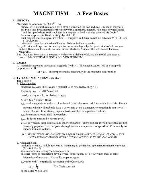
A. HISTORY
Magnetite or lodestone (Fe II OFe III 2O 3 )
mineral in its natural state often has a strong attraction for iron and steel...mined in magnesia
but Pliny says it was named for the discoverer, a shepherd, magnes, "the nails of whose shoes
and the tip of whose staff stuck fast in a magnetick field while he pastured his flocks."
Lodestone appears in Greek writings by 800 B.C.
First magnetic technological invention — compass: in China, sometime between 2637 B.C. and
1100 A.D. (!)
others say it was introduced to China in 1200s by Italians or Arabs
Early theories and experiments on magnetism were developed by the great minds of all times —
Gilbert, Descartes, Coulomb, Poisson, Green, Oertsted, Ampere, Davy, Freesnel, Faraday,
Maxwell...
But: Quantum Mechanics is necessary to develop a viable model, and the model continues to
evolve: MAGNETISM IS NOT A SOLVED PROBLEM
B. BASICS
All materials respond to an external magnetic field (H). The magnetization (M) of a sample is
proportional to H:
M = χH. The proportionality constant, χ, is the magnetic susceptibility
C. TYPES OF MAGNETISM - see chart
The Big five
1. Diamagnetism
electrons in closed shells cause a material to be repelled by H (χ < 0).
Typically, χ m = -1x10 -6 emu/mol
usually a very small contribution to χ exp
χ exp = χ dia + χ para + χ Pauli
χ dia — diamagnetic term due to closed-shell (core) electrons. ALL materials have this. For our
systems, which will probably have a very small χ, the diamagnetic correction is non-trivial —
can be obtained from atom/group additivities or the Curie plot (see below).
χ dia is temperature and field independent.
χ para is due to unpaired electrons (= χ p )
χ Pauli is typically seen in metals and other conductors - due to mixing excited states that are not
thermally populated into the ground (singlet) state - temperature independent. Presumably not
important in our systems.
ALL OTHER TYPES OF MAGNETISM REQUIRE UNPAIRED SPINS (MOMENTS) — THE
INTERACTIONS AMONG SPINS DETERMINES THE TYPE OF MAGNETISM
2. Paramagnetism
randomly oriented, rapidly reorienting moments; no permanent, spontaneous magnetic moment
(M = 0 if H = 0)
spins are non-interacting (non-cooperative)
all other forms of magnetism have a critical temperature, T C , below which there is some
interaction of moments. Above T C ⇒ paramagnet
χ p varies with T empirically according to the Curie Law:
χ p
= C T
or the Curie-Weiss Law:
C = Curie constant

χ p
=
C
θ = Weiss constant
T −θ
θ is indicative of intermolecular interactions among the moments
θ > 0 - ferromagnetic interactions (NOT ferromagnetism)
θ < 0 - antiferromagnetic interactions (NOT antiferromagnetism)
2
DIAMAGNETISM
INCIPIENT
FERROMAGNETISM
METAMAGNETISM
ANTI-
FERROMAGNETISM
FERROMAGNETISM
FERRIMAGNETISM
SPERIMAGNETISM
SUPER-
PARAMAGNETISM
PARAMAGNETISM
SPEROMAGNETISM
ASPEROMAGNETISM
SPIN GLASS
HELIMAGNETISM
MICTOMAGNETISM
Using the Curie Plot:
χ exp
=
C
T −θ + χ T
χ exp
= C T +χ T
(χ T = χ dia + χ Pauli = temperature independent contribution)
(at high temperature if θ is small)

Plot χ exp vs 1/T
0.4
0.35
para
3
0.3
0.25
0.2
0.15
0.1
0.05
Paramagnetic Susceptibility
ferro
antiferro
slope = C; intercept = χ T; ⇒ χ exp - χ T = χ p
...then plot 1/χ p vs. T
0
0 0.1 0.2 0.3 0.4 0.5
1/Temperature (1/K)
50
θ = 0
40
30
20
10
Paramagnetic Susceptibility
θ = +2
θ = -2
slope = 1/C; intercept = θ/C
0
0 5 10 15 20
1/Temperature (1/K)
A magnetometer measures M which gives χ. Do the first plot to get χ T . Then at all T and H, χ p
= χ exp - χ T
The magnetization plot
For an atom with spin m s , its energy in H is:
E(m s
) = m s
gµ B
H µ = -m s gµ B

µ B is Bohr magneton (= 9.27x10 -24 J/T); g is the Lande constant (= 2.0023192778)
Consider N particles, with n i in ith level
∑ n
i i
= N
4
⎛
P i
= n exp − ε i ⎞
⎜ ⎟
kT
i
N = ⎝ ⎠
⎛
exp − ε i ⎞
∑ ⎜ ⎟
i ⎝ kT ⎠
M = N ∑ µ
i i
P i
now, consider two spin states (m s = ± 1/2),
+1/2
⎛
( −m s
gµ B )exp −m s gµ B H ⎞
∑
⎜ ⎟
ms=−1/2
⎝ kT ⎠
M = N
+1/2 ⎛
exp −m s gµ B H ⎞
∑ ⎜ ⎟
ms=−1/2 ⎝ kT ⎠
= Ngµ B
2
= Ngµ B
2
⎡ ⎛
exp gµ B H ⎞ ⎛
⎜ ⎟ − exp − gµ B H ⎞ ⎤
⎜
⎢
⎟
⎝ 2kT ⎠ ⎝ 2kT ⎠
⎥
⎢
⎛
exp⎜
gµ B H ⎞ ⎛
⎟ + exp⎜
− gµ B H ⎥
⎢
⎞
⎟ ⎥
⎣
⎢ ⎝ 2kT ⎠ ⎝ 2kT ⎠ ⎦
⎥
⎛
tanh gµ B H ⎞
⎜ ⎟ since tanh(y) = (e y -e -y )/(e y +e -y )
⎝ 2kT ⎠
if y

a) For x >> 1, B S
x
⎡
( ) − 1 2
( ) = 1 S S+ 1 ⎣ 2
⎤
⎦ = 1
x = gµ B H
kT >> 1 means H T >> k
= 1.38x10−23 J / K
gµ B 2x9.27x10 −24 J/ T = 0.7T / K
b) For x

S=1/2
S=1
S=3/2
S=2
S=5/2
S=3
S=7/2
S=4
S=9/2
S=5
M
molar
( µ B
)
10
9
8
7
6
5
4
6
3
2
1
0
0 1 2 3 4 5 6 7
H/T (Tesla/Kelvin)
The effective magnetic moment
directly relates to number of spins:
µ eff = g[S(S+1)] 1/2 µ B
S µ eff / µ B
1/2 1.73
1 2.83
2 4.89
related to molar susceptibility (χ m = emu/mol)
χ m
= Nµ 2
eff
3kT
= C'
T
µ eff
= 3kC' = 2.82 C'
Therefore,
N
µ eff
= 2.824 χ m
T
3. Ferromagnetism
moments throughout a material in 3-D tend to align parallel
can lead to a spontaneous permanent M (in absence of H)
but, in a macroscopic system, it is energetically favorable for spins to segregate into regions
called DOMAINS - domains need not be aligned with each other
A Domain
may or may not have spontaneous M
application of H causes aligned domains to grow at the expense of misaligned
domains...alignment persists when H is removed

7
Ferromagnetism is a critical phenomenon, involving a phase transition that occurs at a critical
temperature, T c = Curie Temperature. Above T c ⇒ paramagnet
T C is directly proportional to S(S+1)
It takes energy to move domain walls - hysteresis:
M = χH app
Sample Magnetization
M(+)
M sat
H app
(-) (+)
H app
Applied Field M R
2H C
M(-)
M R
= Remnant Magnetization (M at H app
= 0)
M sat
= Saturation Magnetization (M sat
= Ngµ B
S)
H C
= Coercive Field (H app
required to flip M)
"Hard" magnetic material = high Coercivity
"Soft" magnetic material = low Coercivity
Remanence: Magnetization of sample after H is removed
Coercive field: Field required to flip M (+M to -M)
4. Antiferromagnetism
spins tend to align antiparallel in 3-D
no spontaneous M
no permanent M
critical temperature: T N (Neel Temperature)
above T N ⇒ paramagnet
5. Ferrimagnetism
requires two chemically distinct species with different moments
they couple antiferomagnetically:
no M; critical T = T C (Curie Temperature)
bulk behavior very similar to ferromagnetism
Magnetite is a ferrimagnet
6. Other types
M sat = Νgµ B S
Electromagnets
• High M R and Low H C
Electromagnetic Relays
• High M sat , Low M R , and Low H C
Magnetic Recording Materials
• High M R
and relatively High H C
Permanent Magnets
• High M R
and High H C

DIAMAGNETISM
INCIPIENT
FERROMAGNETISM
Low T; temporary alignment of moments
of ions & itinerant electrons
8
METAMAGNETISM
Field-induced transition to magnetic
state;
must be below Neel temperature
ANTI-
FERROMAGNETISM
FERROMAGNETISM
FERRIMAGNETISM
SPERIMAGNETISM
Two species frozen as in speromagnet;
often net magnetication
SUPER-
PARAMAGNETISM
Small particle size allows single
domain fluctuation; destroyed by
cooling below blocking temperature
PARAMAGNETISM
SPEROMAGNETISM
Local moments licked into random
orientation;no net magnetiztion
ASPEROMAGNETISM
As in speromagnetism, but some orientation;
net magnetization
SPIN GLASS
Magnetic ions cooled in a nonmagnetic host;
usually dilute; RKKY coupling only (?)
HELIMAGNETISM
Crystalline asperomagnet
MICTOMAGNETISM
Cluster glass; local correlations dominant
D. SPECIAL TOPICS
1. Magnetooptical Disks
a. Reading
Magnetic materials rotate plane polarized light
in transmission: Faraday effect
in reflection: Kerr effect (used in devices)
Direction of rotation depends on polarization of M
b. Writing
actually a thermo-magnetic process since a high-powered laser is used to heat the sample
1) Curie point writing-heat above T C , then cool in applied field
2) Threshold (or compensation point) writing - if material has a temperature dependent
coercive field heat to point where H > H c , then on cooling H < H c
c. Materials
Typically rare-earth transition metal alloys (RE-TM) RE: Gd, Tb; TM: Fe, Co

9
Many factors to tune: T c , H c , Magnetic anisotropy, reflectivity, Kerr rotation, stability, etc.
2. Spin Glasses — one of the more intriguing new forms of magnetism
may be a new state of matter, maybe not
prototypical SG is an alloy, with 1-10% of a paramagnetic impurity (e.g., Fe or Mn) in a
diamagnetic metal (e.g. Cu or Au)
Spin coupling is mediated through the conduction electrons through the RKKY interaction
(Ruderman, Kittel, Kasuya, Yosida) - oscillatory in nature
A
B
This leads to frustration:
• •
• •
unfrustrated
• ≡ ≡
• •
frustrated
ferromagnetic coupling
antiferromagnetic coupling
• spin center
C
• • • •
• • • •
unfrustrated
frustrated
A critical consequence of Frustration is a highly degenerate ground state - there are
MANY equally probable, equally acceptable combinations of spins
Therefore, even at 0 Kelvin, many states are populated - novel thermodynamic and
magnetic properties
Experimentally, the hallmark of a SG is a cusp in the AC susceptibility - defines a critical
temperature - T SG
Heat capacity measurements do not reveal the some critical temperature
SG do show remanence and hysteresis effects
SG theory has been adopted to other problems, including:
combinatorial optimization (traveling salesman) problems
neural networks
pre-biotic evolution
E. MISCELLANY
1. Units and fundamental constants
N = 6.022 x 10 23 mol -1
g = 2.0023
k = 1.3807 x 10 -23 J/K
µ B = 9.274 x 10 -24 J/T
Nµ B 2 /k = 0.375 emu K/mol
gµ B /k = 1.3449 K/T
G = g 1/2 cm -1/2 s -1
T = 10 4 G
T 2 = 10 J/emu
2. Saturation behavior of S-only paramagnets
M = M sat B S (gµ B H/kT)
B S (x) = (1/S)((S + 1/2)x coth(S + 1/2)x - (x/2) coth(x/2))

M sat = Ngµ B S = 11.18245 S J/mol•T = 1.118245 x 10 4 S emu•G/mol
3. Curie Law for paramagnets
M = χH
χT = C = Ng 2 µ 2 B
S(S +1)
= 0.125g
3k
2 S(S+1) emu•K/mol
µ eff = (g 2 S(S+1) 1/2 = (8χT) 1/2
4. Relation between saturation and Curie behaviors
C( emu •K)
M sat
( emu •G) = Ng 2 µ 2 B
S(S +1)
= gµ (S +1)
B
=
3kNgµ B
S
3k
10
2.0023•9.274x10 −28 J/ G
3•1.3807x10 −23 J / K (S +1) = 4.4831x10 −5 K (S +1)
G
F. MAGNETIC DIMERS – THE HEISENBERG-DIRAC-VAN VLECK HAMILTONIAN
1. Introduction
In section C.2 we examined primary magnetochemistry relationships for paramagnets –
species with non-interacting spins. The magnetic properties of such materials can be described
by the Curie-Weiss law (for small values of H/T), or more generally by:
M = Ngµ B
SB S
However, in the next simplest case – a molecule with two exchange-coupled unpaired
electrons – the magnetic properties cannot usually be described by this relation except at very
low temperatures. This will be the case when the exchange coupling creates thermally accessible
states of different spin multiplicity. Such is the case for most organic biradicals.
The Heisenberg-Dirac-Van Vleck (HDVV) Hamiltonian, eq 1, is an empirical operator that
models interaction (coupling) of unpaired electrons. The form of the Hamiltonian suggests that
coupling arises through interaction of spin angular momentum operators. The magnitude of the
interaction depends on the interaction parameter, J ij (called the exchange parameter). The J ij
term embodies all of the interactions that determine the ground state spin preference. The
product of spin operators is a reasonable component since interaction of species containing
unpaired electrons results in either a decrease (antiferromagnetic coupling) or increase
(ferromagnetic coupling) in spin angular momentum. For example, two doublets can couple to
yield a singlet and a triplet, the relative energies of which depend on J ij . By definition, for
ferromagnetic (high-spin) coupling J ij > 0, while for antiferromagnetic coupling, J ij < 0.
H ˆ ij
= −2J ˆ ij
S ˆ i
S j
(1)
The product of spin angular momentum operators may be expressed in terms of component
and product (total) spin angular momentum operators,
S ˆ 2
Tot
=
⎛
⎝
S ˆ i
+ S ˆ j
therefore, ˆ S i ˆ
2
⎞
⎠ = S ˆ i
+ S ˆ j
+ 2S ˆ ˆ i
S j
(2)
S j
= 1 ⎛
S
2 ˆ 2
Tot
− S ˆ i
−S ˆ 2 ⎞
⎝
j ⎠
(3)
Since the eigenvalue of S ˆ 2 is S( S +1), the energy of the state with spin S Tot
resulting from
interaction of species with spins S i
and S j
is given by,

[ ( ) −S i ( S i
+1) − S j ( S j
+1)
] (4)
E Tot
= −J ij
S Tot
S Tot
+1
Thus for two doublets (2 x multiplicity 2 = 4 states), coupling results in a triplet and a singlet
(multiplicity 3 and multiplicity 1 = 4 states). In the case of ferromagnetic coupling (J > 0), the
energy of the triplet state (S = 1) is,
[ ] = − J 2
E T
= −J 11 ( +1) − 1 1
2( 2 +1 )− 1 1
[ 2( 2 +1 )] = −J 2 − 3 4 − 3 4
The energy of the singlet state (S = 0) is,
[ ] = 3J 2
E S
= −J 0( 0 +1) − 1 1
2
(
2 +1 ) − 1 1
[ 2
(
2 +1 )] = −J 0 − 3 4 − 3 4
The singlet triplet gap, ∆E ST , is given by,
∆E ST
= E S
− E T
= 3J 2 − ( −J
2 ) = 2J (8)
The energy level diagram for ferromagnetic coupling is shown below.
Singlet, S = 0
11
(6)
(7)
S = 1/2
E ST
S = 1/2
Triplet, S = 1
The energy level diagram for antiferromagnetic coupling is shown below.
Triplet, S = 1
S = 1/2
E ST
S = 1/2
Singlet, S = 0
Note that by definition of the Hamiltonian, J < 0 describes antiferromagnetic coupling and J
> 0. Had we defined the Hamiltonian as H ˆ ij = 2J ˆ ij S ˆ i S j
, then J < 0 would be for
ferromagnetically coupled spins. Therefore, when reading the literature, always note the form of
the Hamiltonian to be sure of the nature of the type of exchange coupling.
2. Measuring J by Electron Paramagnetic Resonance Spectroscopy
The intensity of the EPR signal is directly proportional to the paramagnetism which can be
given by the Curie Law,
I EPR
∝χ = C T
(9)

Although the paramagnetism of the triplet follows the Curie Law, the concentration of triplet
is temperature dependent and is given by the Boltzmann distribution,
n T
= [ TRIPLET] n T
+ n rel =
S
⎛
3exp⎜
−ε T ⎞
⎟
⎝ RT ⎠
⎛
3exp⎜
−ε T ⎞
⎟ + exp −ε (10)
⎛
⎜ S ⎞
⎟
⎝ RT ⎠ ⎝ RT ⎠
⎛
Multiplication of the numerator and denominator by exp⎜
ε S ⎞
⎟ , and letting ε
⎝ RT
T - ε S = ∆E ST gives,
⎠
⎛
3exp⎜
−∆E ST ⎞
⎟
⎝ RT ⎠
[ TRIPLET] rel =
1 + 3exp −∆E (11)
⎛
⎜ ST ⎞
⎟
⎝ RT ⎠
Thus, the EPR signal intensity is given by,
12
I EPR
= C T [ TRIPLET]
rel = C T
⎡ ⎛
3exp⎜
−∆E ST ⎞ ⎤
⎟
⎢ ⎝ RT ⎠ ⎥
⎢
⎛
1 +3exp ⎜
−∆E ⎥
ST ⎞
⎢
⎟ ⎥
⎣ ⎝ RT ⎠ ⎦
(12)
A plot of EPR signal intensity versus 1/T for different singlet-triplet gaps is shown below. Note
that very little change in the slope of the plot occurs as the triplet becomes more stable.
0.25
EPR Signal Intensity vs 1/T for Several Values of E TS
∆E = -10 cal
∆E = -5 cal
0.2
∆E = -20 cal
∆E = 5 cal
0.15
∆E = -50 cal
∆E = 10 cal
I EPR
0.1
0.1275 0.255 0.3825 0.51
0.05
∆E = 20 cal
∆E = 50 cal
0
0
1/T (1/K)
3. Measuring J by Magnetometry 1
Van Vleck derived a general equation for calculating paramagnetic susceptibility as a
function of temperature. 2 Use of the equation requires knowledge of the energy levels, which
we calculate with the HDVV Hamiltonian (see previous section). Van Vleck began the

13
derivation by letting the energy levels of the system be developed as a power series expansion in
the applied field.
E n = E n
0 + HEn
(1) + H
2 E n
(2) + H
3 En
(3) +... (13)
The term which is independent of H is the zero-order term (and has units of J, the exchange
parameter), while the term linear in H is the first-order Zeeman term, and the term that scales as
H 2 is the second-order Zeeman term, and so on. Neglecting Zero-field splitting, and assuming
isotropic g, the total magnetic moment, M, for the system is:
( )
∑ µ n exp −E n k B T
n
M = N
∑exp −E n
( kB T)
n
Where µ n is the magnetic moment of state n (µ n = - ∂E n /∂H). Now,
( ) = exp
exp −E n k B T
( )
k B T
(14)
⎡ − E
0
n
+ HEn
(1) + H
2 E
(2)
n
+... ⎤
⎢
⎥ = exp ⎛
⎜
−E 0 n ⎞ ⎛
⎝
⎣
⎦
k B T ⎟ exp −HE (1) n
⎞
⎜
⎟
⎠ ⎝
k B T
... (15)
⎠
Ignoring H 2 and higher-order exponentials, and recalling that for small x,
Then,
⎛
( ) = exp⎜
−E n 0 k B T
exp −E n k B T
⎝
exp(−x) ≅ 1− x
⎞ ⎛
⎟ exp −HE (1) n
⎞ ⎛
⎜
⎟
⎠ ⎝
k B T
...≅ 1 − HE (1)
n
⎞
⎜
⎠ ⎝
k B T
⎠
⎟ exp ⎛
⎜
−E n 0 ⎞
⎝ k B T ⎟ (16)
⎠
(This assumes that first-order Zeeman splitting is much smaller than exchange coupling.) and,
µ n = − δE n
δH = −E n (1) − 2HE n
(2) +... (17)
From the approximation and substitution we obtain,
⎛
(1)
−E n −
(2)
∑( 2HEn ) 1 − HE (1)
⎞
n
⎜
n
⎝
k B T
⎠
⎟ exp ⎛
⎜
−E n 0 ⎞
k B T ⎟
⎝ ⎠
M = N
⎛
1− HE n (1) ⎞
⎜
⎝
k B T
⎠
⎟ exp ⎛
⎜
−E n 0 ⎞
∑
⎝ k B T ⎟
n
⎠
(18)
If we limit the derivation to paramagnetic substances, such that M=0 at H=0, then
(1) ⎛ 0
−E
−E n exp ⎜ n ⎞
∑ ⎟
⎝ k B T
= 0 (19)
n
⎠
Retaining only terms linear in H, and ignoring second-order energy terms, we obtain,

Since χ=M/H, then
Recall that,
14
(1)
( E n ) 2
⎛
∑ exp⎜
−E 0 n
⎞
n k B T
k B T
⎟
⎝ ⎠
M = NH
⎛
exp⎜
−E n 0 ⎞
∑
⎟
⎝ k B T
n
⎠
(20)
(1)
( E n ) 2
⎛
∑ exp⎜
−E n 0 ⎞
n k B T k B T
⎟
⎝ ⎠
χ = N
⎛
exp⎜
−E n 0 ⎞
∑
⎟
⎝ k B T
n
⎠
(21)
+S
(1)
E n = ms gµ B and ∑
2
m s
−S
= 1 3 S ( S +1 )( 2S +1) (22)
and adding degeneracy terms gives,
⎛
χ = Ng 2 µ
2 ∑S( S +1) ( 2S+1)
exp −E ⎞
⎜ S kB T
⎟
B S
⎝ ⎠
3k B T
⎛
( 2S +1)exp −E ⎞
∑ ⎜ S
⎝ k B T
⎟
S
⎠
(23)
Plugging in the constants gives,
χ = 0.125g2 emuK / mol
T
⎛
∑S( S+ 1) ( 2S +1)
exp −E ⎞
⎜ S k
S
⎝ B T
⎟
⎠
⎛
( 2S +1)exp −E ⎞
∑ ⎜ S
⎝ k B T
⎟
S
⎠
(24)
Where E S is the energy of the exchange-coupled spin states determined using the HDVV
Hamiltonian. The energies of the states (in units of J) are relative to the lowest state, which is
taken as zero. The denominator can be modified according to the Curie-Weiss law to give:
= 0.125g2 emuK / mol
T − ( )
∑
S
S( S +1) ( 2S + 1)
⎛
exp −E ⎞
S
⎜
⎝ kB T⎟
⎠
⎛
( 2S +1)exp −E ⎞
S
⎜
⎝ kB T ⎟
S
⎠
∑
(25)
Below are plots of T vs T for = -0.01 K and -500 cm -1 ≤ J ≥ +500 cm -1 .

15
1
χ
paraT
(emu•K/mol)
0.8
0.6
0.4
0.2
-500
-250
-150
-50
-10
-5
+5
+10
+50
+150
+250
+500
0
0 500 1000 1500 2000 2500
Temperature (Kelvin)
Below are plots of vs T for = -0.01 K and -500 cm -1 ≤ J ≥ +500 cm -1 . Note that for
ferromagnetic coupling, increases asymtotically as the temperature is lowered, while for
antiferromagnetic coupling, exhibits a maximum at T max
.
0.005
0.004
χ
para (emu/mol)
0.003
0.002
-500
-250
-150
-50
-10
-5
+5
+10
+50
+150
+250
+500
0.001
0
0 500 1000 1500 2000 2500
Temperature (Kelvin)

The exchange coupling parameter is related to T max
by:
16
|J| = 0.8 kT max
(26)
Thus, a maximum in the plot of
vs. T is the signature of antiferromagnetic coupling.
References
1)Kahn, O. Molecular Magnetism; VCH: New York, 1993.
2)Van Vleck, J. H. The Theory of Electric and Magnetic Susceptibilities; Oxford University
Press: Oxford, 1932.