Day 7 - UH Department of Mathematics

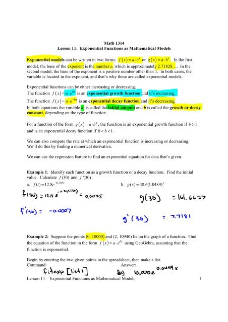
Math 1314
Lesson 11: Exponential Functions as Mathematical Models
x
x
Exponential models can be written in two forms: f ( x) = a ⋅ e or g ( x) a b
= ⋅ . In the first
model, the base of the exponent is the number e, which is approximately 2.71828…. In the
second model, the base of the exponent is a positive number other than 1. In both cases, the
variable is located in the exponent, and that’s why these are called exponential models.
Exponential functions can be either increasing or decreasing.
bx
The function f ( x) = a ⋅ e is an exponential growth function and it’s increasing.
bx
The function f ( x) = a ⋅ e − is an exponential decay function and it’s decreasing.
In both equations the variable a is called the initial amount and b is called the growth or decay
constant, depending on the type of function.
x
For a function of the form g ( x) a b
and is an exponential decay function if 0 < b < 1.
= ⋅ , the function is an exponential growth function if b > 1
We can also compute the rate at which an exponential function is increasing or decreasing.
We’ll do this by finding a numerical derivative.
We can use the regression feature to find an exponential equation for data that’s given.
Example 1: Identify each function as a growth function or a decay function. Find the initial
value. Calculate f (30) and f '(30) .
a.
0.285t
= e −
b. g( x ) = 38.6(1.0489) x
f ( t) 12.8
Example 2: Suppose the points (0, 10000) and (2, 10940) lie on the graph of a function. Find
bx
f x = a ⋅ e using GeoGebra, assuming that the
the equation of the function in the form ( )
function is exponential.
Begin by entering the two given points in the spreadsheet, then make a list.
Command:
Answer:
Lesson 11 – Exponential Functions as Mathematical Models 1

Uninhibited Exponential Growth
Some common exponential applications model uninhibited exponential growth. This means
that there is no “upper limit” on the value of the function. It can simply keep growing and
growing. Problems of this type include population growth problems and growth of investment
assets.
Example 3: A biologist wants to study the growth of a certain strain of bacteria. She starts
with a culture containing 25,000 bacteria. After three hours, the number of bacteria has grown to
63,000. Assume the population grows exponentially and the growth is uninhibited.
bx
a. Find the equation of the function in the form f ( x) = a ⋅ e using GGB.
State the two points given in the problem.
Enter the two points in the spreadsheet, then make a list.
Command:
Answer:
b. How many bacteria will be present in the culture 6 hours after she started her study?
Example 4: The sales from company ABC for the years 1998 – 2003 are given below.
Year 1998 1999 2000 2001 2002 2003
profits in millions of dollars 51.4 53.2 55.8 56.1 58.1 59.0
Rescale the data so that x = 0 corresponds to 1998. Begin by making a list.
a. Find an exponential regression model for the data.
Command:
Answer:
b. Find the rate at which the company's sales were changing in 2007.
Command:
Answer:
Lesson 11 – Exponential Functions as Mathematical Models 2

Exponential Decay
Example 5: At the beginning of a study, there are 50 grams of a substance present. After 17
days, there are 38.7 grams remaining. Assume the substance decays exponentially.
a. State the two points given in the problem.
Enter the two points in the spreadsheet and make a list.
b. Find an exponential regression model.
Command:
Answer:
c. What will be the rate of decay on day 40 of the study?
Command:
Answer:
Exponential decay problems frequently involve the half-life of a substance. The half-life of a
substance is the time it takes to reduce the amount of the substance by one-half.
Example 6: A certain drug has a half-life of 4 hours. Suppose you take a dose of 1000
milligrams of the drug.
a. State the two points given in the problem.
Enter the two points in the spreadsheet and make a list.
b. Find an exponential regression model.
Command:
Answer:
c. How much of it is left in your bloodstream 28 hours later?
Command:
Answer:
Lesson 11 – Exponential Functions as Mathematical Models 3

Example 7: The half-life of Carbon 14 is 5770 years.
a. State the two points given in the problem.
Enter the two points in the spreadsheet and make a list.
b. Find an exponential regression model.
Command:
Answer:
c. Bones found from an archeological dig were found to have 22% of the amount of Carbon 14
that living bones have. Find the approximate age of the bones.
Command:
Answer:
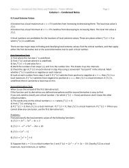
Limited Growth Models
Some exponential growth is limited; here’s an example:
A worker on an assembly line performs the same task repeatedly throughout the workday. With
experience, the worker will perform at or near an optimal level. However, when first learning to
do the task, the worker’s productivity will be much lower. During these early experiences, the
worker’s productivity will increase dramatically. Then, once the worker is thoroughly familiar
with the task, there will be little change to his/her productivity.
The function that models this situation will have the form Q( t)
= C − Ae −kt .
This model is called a learning curve and the graph of the function will look something like
this:
The graph will have a y intercept at C – A and a horizontal asymptote at y = C. Because of the
horizontal asymptote, we know that this function does not model uninhibited growth.
Lesson 11 – Exponential Functions as Mathematical Models 4

Example 8: Suppose your company’s HR department determines that an employee will be able
0.5t
to assemble Q( t) = 50 − 30e − products per day, t months after the employee starts working on
the assembly line. Enter the function in GGB.
a. How many units can a new employee assemble as s/he starts the first day at work?
b. How many units should an employee be able to assemble after two months at work?
c. How many units should an experienced worker be able to assemble?
d. At what rate is an employee’s productivity changing 4 months after starting to work?
Logistic Functions
The last growth model that we will consider involves the logistic function. The general form of
A
the equation is Q( t)
= and the graph looks something like this:
kt
1 + Be −
If we looked at this graph up to around x = 2 and didn’t consider the rest of it, we might think
that the data modeled was exponential. Logistic functions typically reach a saturation point – a
point at which the growth slows down and then eventually levels off. The part of this graph to
the right of x = 2 looks more like our learning curve graph from the last example. Logistic
functions have some of the features of both types of models.
Note that the graph has a limiting value at y = 5. In the context of a logistic function, this
asymptote is called the carrying capacity. In general the carrying capacity is A from the
formula above.
Lesson 11 – Exponential Functions as Mathematical Models 5

Logistic curves are used to model various types of phenomena and other physical situations such
as population management. Suppose a number of animals are introduced into a protected game
reserve, with the expectation that the population will grow. Various factors will work together to
keep the population from growing exponentially (in an uninhibited manner). The natural
resources (food, water, protection) may not exist to support a population that gets larger without
bound. Often such populations grow according to a logistic model.
Example 9: A population study was commissioned to determine the growth rate of the fish
population in a certain area of the Pacific Northwest. The function given below models the
population where t is measured in years and N is measured in millions of tons. Enter the
function in GGB.
2.4
N( t)
=
0.338t
1 + 2.39e −
a. What was the initial number of fish in the population?
b. What is the carrying capacity in this population?
c. What is the fish population after 3 years?
d. How fast is the fish population changing after 2 years?
Lesson 11 – Exponential Functions as Mathematical Models 6

Math 1314
Lesson 12
Curve Analysis (Polynomials)
This lesson will cover analyzing polynomial functions using GeoGebra.
Suppose your company embarked on a new marketing campaign and was able to track sales
based on it. The graph below gives the number of sales in thousands shown t days after the
campaign began.
Now suppose you are assigned to analyze this information. We can use calculus to answer the
following questions:
When are sales increasing or decreasing? (Note that the graph stops at t = 40.)
What is the maximum number of sales in the given time period?
Where does the growth rate change?
Etc.
Calculus can’t answer the “why” questions, but it can give you some information you need to
start that inquiry.
There will be several features of a polynomial function that we’ll need to find. Let’s start with a
few College Algebra topics.
An example of a polynomial function is
f ( x) ( x 2)( x 1) ( x 1)
3 2
= − − + . Its graph looks like:
*The domain of any polynomial function is ( ) , −∞ ∞ . Polynomial functions have no asymptotes.
*To find the roots/zeros/x-intercepts/solutions of any function, set the function equal to zero and
solve for x. Or you may simply use the root or roots command in GGB.
*To find the y-intercept for any function, set x = 0 and calculate.
*The range of any polynomial is easier found by looking at the graph of the function.
Lesson 12 – Curve Analysis (Polynomials) 1

3 2
Example 1: Let f ( x) = x − 3x − 13x
+ 15 . Enter the function in GGB.
a. Find any x-intercepts of the function.
Command:
Answer:
b. Find any y-intercept of the function.
Command:
Answer:
Intervals on Which a Function is Increasing/Decreasing
Definition: A function is increasing on an interval (a, b) if, for any two numbers x1
and x2
in
(a, b), f ( x1 ) < f ( x2
) , whenever x
1
< x2
. A function is decreasing on an interval (a, b) if, for
any two numbers x1
and x
2
in (a, b), f ( x1 ) > f ( x2
) , whenever x
1
< x2
.
In other words, if the y values are getting bigger as we move from left to right across the graph of
the function, the function is increasing. If they are getting smaller, then the function is
decreasing. We will state intervals of increase/decrease using interval notation. The interval
notation will consists of corresponding x-values wherever y-values are getting bigger/smaller.
Example 2: Given the following graph of a function, state the intervals on which the function is:
a. increasing. b. decreasing.
We can use calculus to determine intervals of increase and intervals of decrease. A function can
change from increasing to decreasing or from decreasing to increasing at its critical numbers, so
we start with a definition of critical numbers:
The critical numbers of a polynomial function are all values of x that are in the domain of f
where f ′( x) = 0 (the tangent line to the curve is horizontal).
A function is increasing on an interval if the first derivative of the function is positive for every
number in the interval. A function is decreasing on an interval if the first derivative of the
function is negative for every number in the interval.
Lesson 12 – Curve Analysis (Polynomials) 2

Example 3: The graph given below is the first derivative of a function, f. Find:
a. any critical numbers.
b. any intervals where the function is increasing/decreasing.
5 4
Example 4: Let f ( x)
= x − x , find:
a. any critical numbers.
b. any intervals where the function is increasing/decreasing.
Lesson 12 – Curve Analysis (Polynomials) 3

To find the intervals on which a given polynomial function is increasing/decreasing using
GGB:
1. Use GGB to graph the derivative of the function.
′ = ;
2. Find any critical numbers. (Recall that the critical numbers occur whenever f ( x) 0
hence, simply find the zeros of f ′ .)
2. Create a number line, subdividing the line using the critical numbers.
3. Use the graph of the derivative (or compute the value of a test point) to determine the sign
(positive or negative) of the y values of the derivative in each interval and record this on your
number line.
4. In each interval in which the derivative is positive, the function is increasing. In each interval
in which the derivative is negative, the function is decreasing.
5 2
Example 5: Let f ( x) = x − 16x + 4x
. Using GGB find:
a. any critical numbers.
Command:
Answer:
b. any intervals where the function is increasing/decreasing.
Relative Extrema
The relative extrema are the high points and the low points of a function. A relative maximum
is higher than all of the points near it; a relative minimum is lower than all of the points near it.
A relative maximum or a relative minimum can only occur at a critical number.
Lesson 12 – Curve Analysis (Polynomials) 4

You can use the same number line that you created to determine intervals of increase/decrease to
find the x coordinate of any relative extrema. Use these three statements to determine if a critical
number generates a relative extremum. Once you find that x = c generates a relative extremum,
you can find the y coordinate of the relative extremum by computing f ( c ) or for a more
accurate answer use the extremum command in GGB.
1. If the sign of the derivative changes from positive to negative at a critical number, x = c , then
c,
f c .
the function has a relative maximum at the point ( ( ))
2. If the sign of the derivative changes from negative to positive at a critical number, x = c , then
c,
f c .
the function has a relative minimum at the point ( ( ))
3. If the sign of the derivative does not change sign at a critical number, x = c , then the function
c,
f c .
has neither a relative maximum nor a relative minimum at the point ( ( ))
Example 6: Find any relative maximum and relative minimum for
5 4
= − .
f ( x)
x x
Example 7: Find any relative extrema:
Command:
f x = x + x +
Answer:
6
( ) 0.25 4
Lesson 12 – Curve Analysis (Polynomials) 5

Concavity
In business, for example, the first derivative might tell us that our sales are increasing, but the
second derivative will tell us if the pace of the increase is increasing or decreasing.
From these graphs, you can see that the shape of the curve change differs depending on whether
the slopes of tangent lines are increasing or decreasing. This is the idea of concavity.
Example 8: The graph given below is the graph of a function f. Determine the interval(s) on
which the function is concave upward and the interval(s) on which the function is concave
downward.
We find concavity intervals by analyzing the second derivative of the function. The analysis is
very similar to the method we used to find increasing/decreasing intervals.
1. Use GeoGebra to graph the second derivative of the function. Then find the zero(s) of the
second derivative.
2. Create a number line and subdivide it using the zeros of the second derivative.
3. Use the graph of the second derivative to determine the sign (positive or negative) of the y
values of the second derivative in each interval and record this on your number line.
4. In each interval in which the second derivative is positive, the function is concave upward. In
each interval in which the second derivative is negative, the function is concave downward.
Lesson 12 – Curve Analysis (Polynomials) 6

Example 9: State intervals on which the function is concave upward and intervals on which the
1 5 2 2
function is concave downward: f ( x) = x − x −8x
− 1
2 3
Command:
You’ll also need to be able to identify the point(s) where concavity changes. A point where
concavity changes is called a point of inflection.
You can use the same number line that you created to determine concavity intervals to find the x
coordinate of any inflection points. Use the following two statements to determine if a zero of
the second derivative generates an inflection point.
1. If the sign of the second derivative changes from positive to negative or from negative to
positive at a number, x c
c,
f c .
= , then the function has an inflection point at the point ( ( ))
2. If the sign of the second derivative does not change sign at a number, x = c , then the function
c,
f c .
does not have an inflection point at the point ( ( ))
Once you find that x = c generates an inflection point, you can find the y coordinate of the
inflection point by computing f ( c ).
Example 10: Given
1 5 2 2
f ( x) = x − x −8x
− 1, find any inflection points.
2 3
Example 11: Given
Command:
3 2
f ( x)
= x − 3x
− 24x
+ 32 , find any inflection points.
Answer:
Lesson 12 – Curve Analysis (Polynomials) 7