Well-conditioned boundary integral formulations for the ... - Njit

D N C k A k,Sik/2 B k,2,k,0.4H 2/3 k 1/3
Mem Time/It Mem Time/It Mem Time/It
10.2 λ 47,628 0.1 Gb 0.61 m 0.16 Gb 0.93 m 0.22 Gb 1.38 m
20.4 λ 193,548 0.4 Gb 3.46 m 0.64 Gb 5.40 m 0.88 Gb 8.10 m
30.6 λ 437,772 0.9 Gb 9.63 m 1.44 Gb 15.84 m 1.98 Gb 23.64 m
40.8 λ 780,300 1.6 Gb 19.55 m 2.5 Gb 31.03 m 3.5 Gb 47.58 m
51.0 λ 1,175,628 2.5 Gb 37.03 m 3.9 Gb 62.62 m 5.5 Gb 90.60 m
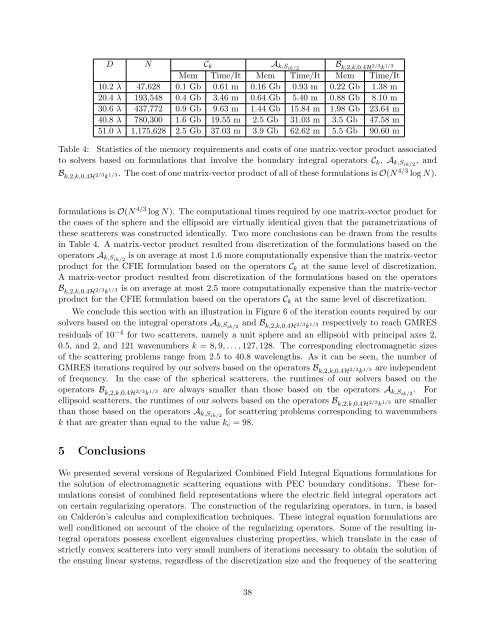
Table 4: Statistics of the memory requirements and costs of one matrix-vector product associated
to solvers based on formulations that involve the boundary integral operators C k , A k,Sik/2 , and
B k,2,k,0.4H 2/3 k 1/3. The cost of one matrix-vector product of all of these formulations is O(N 4/3 log N).
formulations is O(N 4/3 log N). The computational times required by one matrix-vector product for
the cases of the sphere and the ellipsoid are virtually identical given that the parametrizations of
these scatterers was constructed identically. Two more conclusions can be drawn from the results
in Table 4. A matrix-vector product resulted from discretization of the formulations based on the
operators A k,Sik/2 is on average at most 1.6 more computationally expensive than the matrix-vector
product for the CFIE formulation based on the operators C k at the same level of discretization.
A matrix-vector product resulted from discretization of the formulations based on the operators
B k,2,k,0.4H 2/3 k 1/3 is on average at most 2.5 more computationally expensive than the matrix-vector
product for the CFIE formulation based on the operators C k at the same level of discretization.
We conclude this section with an illustration in Figure 6 of the iteration counts required by our
solvers based on the integral operators A k,Sik/2 and B k,2,k,0.4H 2/3 k1/3 respectively to reach GMRES
residuals of 10 −4 for two scatterers, namely a unit sphere and an ellipsoid with principal axes 2,
0.5, and 2, and 121 wavenumbers k = 8, 9, . . . , 127, 128. The corresponding electromagnetic sizes
of the scattering problems range from 2.5 to 40.8 wavelengths. As it can be seen, the number of
GMRES iterations required by our solvers based on the operators B k,2,k,0.4H 2/3 k1/3 are independent
of frequency. In the case of the spherical scatterers, the runtimes of our solvers based on the
operators B k,2,k,0.4H 2/3 k 1/3 are always smaller than those based on the operators A k,S ik/2
. For
ellipsoid scatterers, the runtimes of our solvers based on the operators B k,2,k,0.4H 2/3 k 1/3 are smaller
than those based on the operators A k,Sik/2 for scattering problems corresponding to wavenumbers
k that are greater than equal to the value k c = 98.
5 Conclusions
We presented several versions of Regularized Combined Field Integral Equations formulations for
the solution of electromagnetic scattering equations with PEC boundary conditions. These formulations
consist of combined field representations where the electric field integral operators act
on certain regularizing operators. The construction of the regularizing operators, in turn, is based
on Calderón’s calculus and complexification techniques. These integral equation formulations are
well conditioned on account of the choice of the regularizing operators. Some of the resulting integral
operators possess excellent eigenvalues clustering properties, which translate in the case of
strictly convex scatterers into very small numbers of iterations necessary to obtain the solution of
the ensuing linear systems, regardless of the discretization size and the frequency of the scattering
38