Growth of the Original Tail in Anolis grahami: Isometry of the Whole ...
Growth of the Original Tail in Anolis grahami: Isometry of the Whole ...
Growth of the Original Tail in Anolis grahami: Isometry of the Whole ...

Create successful ePaper yourself
Turn your PDF publications into a flip-book with our unique Google optimized e-Paper software.
234 P. J: BERGMANN AND A. P. RUSSELL<br />
ma1 distribution (mnd), that <strong>the</strong> sample is random,<br />
and that <strong>the</strong> data are l<strong>in</strong>ear (Pimentel,<br />
1979). Log-transformation l<strong>in</strong>earizes <strong>the</strong> data<br />
and helps to approximate <strong>the</strong> mnd (Pimentel,<br />
1979). Although it is difficult to take a truly random<br />
biological sample, <strong>the</strong> assumption <strong>of</strong> randomness<br />
is safe because <strong>of</strong> <strong>the</strong> general repeatability<br />
<strong>of</strong> biological studies (Pimentel, 1979). A<br />
multivariate normal distribution, although not<br />
practically testable, is a conservative assumption<br />
(Pimentel, 1979).<br />
The mean vertebral count for <strong>the</strong> entire sample<br />
<strong>of</strong> <strong>in</strong>dividuals with orig<strong>in</strong>al tails was 39.5<br />
(SD = 0.937, range 3842), and <strong>the</strong> mode was<br />
39. Us<strong>in</strong>g <strong>the</strong> modal number would have resulted<br />
<strong>in</strong> a subsample <strong>of</strong> only 15 <strong>in</strong>dividuals.<br />
Thus, all specimens were reta<strong>in</strong>ed for <strong>the</strong> analysis,<br />
with vertebrae 3942 be<strong>in</strong>g excluded from<br />
exam<strong>in</strong>ation. In this way, vertebral number was<br />
standardized at 38, with comparisons be<strong>in</strong>g run<br />
for <strong>the</strong>se first 38 vertebrae. which we have regarded<br />
as iterative homoiogues (Haszprunar,<br />
1991; Roth, 1994). For <strong>the</strong>se analyses, lengths <strong>of</strong><br />
each adjacent pair <strong>of</strong> caudal vertebrae were<br />
comb<strong>in</strong>ed (<strong>the</strong> sacrum is already two vertebrae),<br />
decreas<strong>in</strong>g <strong>the</strong> number <strong>of</strong> variables (p) to 20.<br />
This permitted <strong>the</strong> sample size (N = 30) to exceed<br />
<strong>the</strong> number <strong>of</strong> variables or measurements<br />
(p > N; Pimentel, 1979).<br />
Component load<strong>in</strong>gs <strong>of</strong> pr<strong>in</strong>cipal components<br />
were standardized by divid<strong>in</strong>g by <strong>the</strong> square<br />
root <strong>of</strong> <strong>the</strong> eigenvalue to give allometric load<strong>in</strong>gs<br />
(Pimentel, 1979). The squared (standardized)<br />
allometric load<strong>in</strong>gs sum to one (Shea,<br />
1985) and are proportional to growth (Pimentel,<br />
1979). Allometric component correlations were<br />
determ<strong>in</strong>ed by multiply<strong>in</strong>g <strong>the</strong> allometric load<strong>in</strong>gs<br />
by <strong>the</strong> square root <strong>of</strong> <strong>the</strong> eigenvalue and<br />
divid<strong>in</strong>g <strong>the</strong> product by <strong>the</strong> standard deviation<br />
<strong>of</strong> each variable (Pimentel, 1979). Variance expla<strong>in</strong>ed<br />
by each component for each variable<br />
was calculated by multiply<strong>in</strong>g <strong>the</strong> squared allometric<br />
load<strong>in</strong>g by <strong>the</strong> eigenvalue and divid<strong>in</strong>g<br />
<strong>the</strong> product by variance <strong>of</strong> <strong>the</strong> given variable,<br />
S,,' sensu Pimentel (1979). The contribution <strong>of</strong><br />
each <strong>in</strong>dividual to each component was also determ<strong>in</strong>ed<br />
accord<strong>in</strong>g to Pimentel (1979).<br />
Sexes were also compared with respect to<br />
each pr<strong>in</strong>cipal component by ANOVA or Kruskal-Wallis<br />
tests on <strong>the</strong> specimen component<br />
scores for that component, as appropriate (Pimentel,<br />
1979; Adams, 1998). Allometric component<br />
correlations were tested for significance by<br />
comput<strong>in</strong>g <strong>the</strong> correspond<strong>in</strong>g Pearson's correlation<br />
coefficients (Pimentel, 1979; Tissot, 1988).<br />
The first pr<strong>in</strong>cipal component (PC-I), generally<br />
<strong>in</strong>terpreted as represent<strong>in</strong>g changes <strong>in</strong> shape<br />
that are size dependent (Pimentel, 1979; McK<strong>in</strong>ney<br />
and McNamara, 1991), was tested for isometry,<br />
us<strong>in</strong>g (p-I 2, as a value for isometry and<br />
SVL (mm)<br />
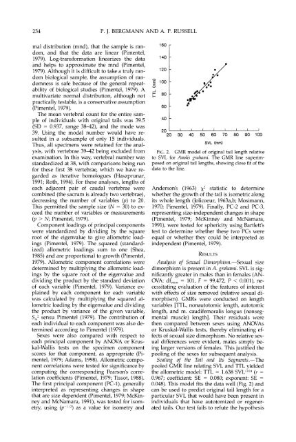
FIG.2. GMR model <strong>of</strong> orig<strong>in</strong>al tail length relati\.e<br />
to SVL for Aizolis yrnlmiili. The GMR l<strong>in</strong>e superimposed<br />
on orig<strong>in</strong>al tail lengths, show<strong>in</strong>g close fit <strong>of</strong> <strong>the</strong><br />
data to <strong>the</strong> l<strong>in</strong>e.<br />
Anderson's (1963) x2 statistic to determ<strong>in</strong>e<br />
whe<strong>the</strong>r <strong>the</strong> growth <strong>of</strong> <strong>the</strong> tail is isometric along<br />
its whole length (Jolicoeur, 1963a,b; Mosimann,<br />
1970; Pimentel, 1979). F<strong>in</strong>ally, PC-2 and PC-3,<br />
represent<strong>in</strong>g size-<strong>in</strong>dependent changes <strong>in</strong> shape<br />
(Pimentel, 1979; McK<strong>in</strong>ney and McNamara,<br />
1991), were tested for sphericity us<strong>in</strong>g Bartlett's<br />
test to determ<strong>in</strong>e whe<strong>the</strong>r <strong>the</strong>se two PCs were<br />
equal or whe<strong>the</strong>r <strong>the</strong>y could be <strong>in</strong>terpreted as<br />
<strong>in</strong>dependent (Pimentel, 1979).<br />
Analysis <strong>of</strong> Sexual Dimorpiiism.-Sexual size<br />
dimorphism is present <strong>in</strong> A. grai~~n~i. SVL is significantly<br />
greater <strong>in</strong> males than <strong>in</strong> females (AN-<br />
OVA: df ,,,,, = 101, F = 99.472, P < 0.001), necessitat<strong>in</strong>g<br />
evaluation <strong>of</strong> <strong>the</strong> features <strong>of</strong> <strong>in</strong>terest<br />
with effects <strong>of</strong> size removed (relative sexual dimorphism).<br />
CMRs were conducted on length<br />
variables [TTL, nonautotomic length, autotomic<br />
length, and m. caudifemoralis longus (nonsegmental<br />
muscle) length]. Their residuals were<br />
<strong>the</strong>n compared between sexes us<strong>in</strong>g ANOVAs<br />
or Kruskal-Wallis tests, <strong>the</strong>reby elim<strong>in</strong>at<strong>in</strong>g effects<br />
<strong>of</strong> sexual size dimorphism. No relative sexual<br />
differences were evident, males simply be<strong>in</strong>g<br />
larger versions <strong>of</strong> females. This justified <strong>the</strong><br />
pool<strong>in</strong>g <strong>of</strong> <strong>the</strong> sexes for subsequent analysis.<br />
Scalirlg <strong>of</strong> ti^ <strong>Tail</strong> and Its Seg111ents.-The<br />
pooled CMR l<strong>in</strong>e relat<strong>in</strong>g SVL and TTL yielded<br />
<strong>the</strong> allometric model: TTL = 1.638 SVL1"'-' (r =<br />
0.967; coefficient: SE = 0.080; exponent: SE =<br />
0.048). This model fits <strong>the</strong> data well (Fig. 2) and<br />
can be used to predict orig<strong>in</strong>al tail length for a<br />
particular SVL that would have been present <strong>in</strong><br />
<strong>in</strong>dividuals that have autotomized or regenerated<br />
tails. Our test fails to refute <strong>the</strong> hypo<strong>the</strong>sis