Elastic Task Model For Adaptive Rate Control

Proceedings of the IEEE Real-Time Systems Symposium, Madrid, Spain, December 1998. 1 

Elastic Task Model For Adaptive Rate Control 

Giorgio C. Buttazzo, Giuseppe Lipari, and Luca Abeni 

Scuola Superiore S. Anna, Pisa, Italy 

giorgio,lipari¡ @sssup.it, luca@hartik.sssup.it 

Abstract 

An increasing number of real-time applications, related 

to multimedia and adaptive control systems, require greater 

flexibility than classical real-time theory usually permits. 

In this paper we present a novel periodic task model, in 

which tasks’ periods are treated as springs, with given elastic 

coefficients. Under this framework, periodic tasks can 

intentionally change their execution rate to provide different 

quality of service, and the other tasks can automatically 

adapt their periods to keep the system underloaded. The 

proposed model can also be used to handle overload conditions 

in a more flexible way, and provide a simple and 

efficient mechanism for controlling the quality of service of 

the system as a function of the current load. 

1. Introduction 

Periodic activities represent the major computational demand 

in many real-time applications, since they provide a 

simple way to enforce timing constraints through rate control. 

For instance, in digital control systems, periodic tasks 

are associated with sensory data acquisition, low-level servoing, 

control loops, action planning, and system monitoring. 

In such applications, a necessary condition for guaranteeing 

the stability of the controlled system is that each 

periodic task is executed at a constant rate, whose value is 

computed at the design stage based on the characteristics of 

the environment and on the required performance. For critical 

control applications (i.e., those whose failure may cause 

catastrophic consequences), the feasibility of the schedule 

has to be guaranteed a priori and no task can change its 

period while the system is running. 

Such a rigid framework in which periodic tasks operate is 

also determined by the schedulability analysis that must be 

performed on the task set to guarantee its feasibility under 

the imposed constraints. To simplify the analysis, in fact, 

some feasibility tests for periodic tasks are based on quite 

rigid assumptions. For example, in the original Liu and 

Layland’s paper [7] on the Rate Monotonic (RM) and the 

Earliest Deadline First (EDF) algorithms, a periodic ¢¤£ task 

is modeled as a cyclical processor activity characterized by 

two parameters, the computation ¥ £ time and period¦ £ the , 

which are considered to be constant for all task instances. 

This is a reasonable assumption for most real-time control 

systems, but it can be too restrictive for other applications. 

For example, in multimedia systems timing constraints 

can be more flexible and dynamic than control theory usually 

permits. Activities such as voice sampling, image acquisition, 

sound generation, data compression, and video playing, 

are performed periodically, but their execution rates are 

not as rigid as in control applications. Missing a deadline 

while displaying an MPEG video may decrease the quality 

of service (QoS), but does not cause critical system faults. 

Depending on the requested QoS, tasks may increase or decrease 

their execution rate to accommodate the requirements 

of other concurrent activities. 

If a multimedia task manages compressed frames, the 

time for coding/decoding each frame can vary significantly, 

hence the worst-case execution time (WCET) of the task can 

be much bigger than its mean execution time. Since hard 

real-time tasks are guaranteed based on their WCET (and 

not based on mean execution times), multimedia activities 

can cause a waste of the CPU resource, if treated as “rigid” 

hard real-time tasks. 

In order to provide theoretical support for such applications, 

some work has been done to deal with tasks with 

variable computation times. In [18] a probabilistic guarantee 

is performed on tasks whose execution times have known 

distribution. In [17], the authors provide an upper bound 

of completion times of jobs chains with variable execution 

times and arbitrary release times. In [9], a guarantee is 

computed for tasks whose jobs are characterized by variable 

computation times and interarrival times, occurring with a 

cyclical pattern. In [8], a capacity reservation technique 

is used to handle tasks with variable computation time and 

bound their computational demand. 

Even in some control application, there are situations in 

which periodic tasks could be executed at different rates in 

different operating conditions. For example, in a flight control 

system, the sampling rate of the altimeters is a function


of the current altitude of the aircraft: the lower the altitude, 

the higher the sampling frequency. A similar need arises 

in robotic applications in which robots have to work in unknown 

environments where trajectories are planned based 

on the current sensory information. If a robot is equipped 

with proximity sensors, in order to maintain a desired performance, 

the acquisition rate of the sensors must increase 

whenever the robot is approaching an obstacle. 

In other situations, the possibility of varying tasks’ rates 

increases the flexibility of the system in handling overload 

conditions, providing a more general admission control 

mechanism. For example, whenever a new task cannot be 

guaranteed by the system, instead of rejecting the task, the 

system can try to reduce the utilizations of the other tasks (by 

increasing their periods in a controlled fashion) to decrease 

the total load and accommodate the new request. Unfortunately, 

there is no uniform approach for dealing with these 

situations. For example, Kuo and Mok [4] propose a load 

scaling technique to gracefully degrade the workload of a 

system by adjusting the periods of processes. In this work, 

tasks are assumed to be equally important and the objective 

is to minimize the number of fundamental frequencies to 

improve schedulability under static priority assignments. In 

[12], Nakajima and Tezuka show how a real-time system 

can be used to support an adaptive application: whenever 

a deadline miss is detected, the period of the failed task is 

increased. In [13], Seto et al. change tasks’ periods within 

a specified range to minimize a performance index defined 

over the task set. This approach is effective at a design 

stage to optimize the performance of a discrete control system, 

but cannot be used for on-line load adjustment. In [6], 

Lee, Rajkumar and Mercer propose a number of policies to 

dynamically adjust the tasks’ rates in overload conditions. 

In [1], Abdelzaher, Atkins, and Shin present a model for QoS 

negotiation to meet both predictability and graceful degradation 

requirements in cases of overload. In this model, the 

QoS is specified as a set of negotiation options, in terms 

of rewards and rejection penalties. In [10, 11], Nakajima 

shows how a multimedia activity can adapt its requirements 

during transient overloads by scaling down its rate or its 

computational demand. However, it is not clear how the the 

QoS can be increased when the system is underloaded. 

Although these approaches may lead to interesting results 

in specific applications, we believe that a more general 

framework can be used to avoid a proliferation of policies 

and treat different applications in a uniform fashion. 

In this paper we present a novel framework, the elastic 

model, which has the following advantages: 

it allows tasks to intentionally change their execution 

rate to provide different quality of service; 

it can handle overload situations in a more flexible 

way; 

it provides a simple and efficient method for controlling 

the quality of service of the system as a function 

of the current load. 

The rest of the paper is organized as follows. Section 

2 presents the elastic task model. Section 3 illustrates the 

equivalence of the model with a mechanical system of linear 

springs. Section 4 describes the guarantee algorithm for a set 

of elastic tasks. Section 5 presents some theoretical results 

which validate the proposed model. Section 6 illustrates 

some experimental results achieved on the HARTIK kernel. 

Finally, Section 7 contains our conclusions and future work. 

2. The elastic model 

The basic idea behind the elastic model proposed in this 

paper is to consider each task as flexible as a spring with a 

given rigidity coefficient and length constraints. In particular, 

the utilization of a task is treated as an elastic parameter, 

whose value can be modified by changing the period or 

the computation time. To simplify the presentation of the 

model, in this paper we assume that the computation is fixed, 

while the period can be varied within a specified range. 

Each task is characterized by five parameters: a computation 

¥ £ time , a nominal ¦ £ period 0, a minimum period 

£¢¡¤£¢¥ , a maximum period ¦ £¦¡¨§© , and an elastic coefficient 

 

¦ 

 

0, which specifies the flexibility of the task to vary its 

£ 

utilization for adapting the system to a new feasible rate configuration. 

The greater £ , the more elastic the task. Thus, 

an elastic task is denoted as: 

 

£ ¥ £ ¦ £ 

0 ¦ £¦¡¤£¥ ¦ £¦¡¨§© 

£ 

¢ 

In the following, ¦ £ will denote the actual period of task 

¢ £ , which is constrained to be in the range ¦ £ ¡¤£¥ ¦ £ ¡¨§© . 

Any task can vary its period according to its needs within 

the specified range. Any variation, however, is subject to 

an elastic guarantee and is accepted only if there exists a 

feasible schedule in which all the other periods are within 

their range. Consider, for example, a set of three tasks, 

whose parameters are shown in Table 1. With the nominal 

periods, the task set is schedulable by EDF since 

10 10 15 

20 40 70 

0 964 

If task ¢ 3 reduces its period to 50, no feasible schedule 

exists, since the utilization would be greater than 1: 

10 

20 

10 

40 

15 

50 

1 05 

However, notice that a feasible schedule exists ( 0 977) 

for !" 1 22, ¦ 2 45, and ¦ 3 50, hence the system can 

¦ 

accept the higher request rate ¢ of 3 by slightly decreasing 

1 

1


¥ £ ¦ £ Task ¦ 

0 

£ ¡¤£¥ ¦ £ ¡¨§ © 

¢ 

¢ 

1 10 20 20 25 1 

2 10 40 40 50 1 

¢ 3 15 70 35 80 1 

Table 1. Task set parameters used for the example. 

the rates of ¢ 1 and ¢ 2. Task ¢ 3 can even run with a period 

3 40, since a feasible schedule exists with periods ¦ 1 

¦ 

¦ and 2 within their range. In when¦ fact, 1 ¦ 24, 2 50, 

3 40, 0 992. Finally, notice that if ¢ 3 requires 

and¦ 

to run with a ¦ period 3 35, there is no feasible schedule 

periods¦ with and¦ 1 2 within their range, hence the request 

3 to execute with a period¦ 3 35 must be rejected. 

of¢ 

Clearly, for a given value of¦ 3, there can be many different 

period configurations which lead to a feasible schedule, 

hence one of the possible feasible configurations must be 

selected. The great advantage of using an elastic model is 

that the policy for selecting a solution is implicitly encoded 

in the elastic coefficients provided by the user. Thus, each 

task is varied based on its current elastic status and a feasible 

configuration is found, if there exists one. 

As another example, consider the same set of three tasks 

with their nominal periods, but suppose that a new periodic 

task ¢ 4 5 30 30 30 0 enters the system at time ¡ . In a 

rigid scheduling framework,¢ 4 (or some other task selected 

by a more sophisticated rejection policy) must be rejected, 

because the new task set is not schedulable, being 

 

4 

¢ 

1 £¤£ 

£ ¥ 

£ 

0 

¦ 

1 131 

Using an elastic model, ¢ however, 4 can be accepted if 

the periods of the other tasks can be increased in such a 

way that the total utilization is less than one and all the 

periods are within their range. In our specific example, the 

period configuration given ¦ by 1 ¦ 23, 2 ¦ 50, 3 80, 

4 30, creates a total utilization 0 989, hence ¢ 4 

¦ 

can be accepted. 

The elastic model also works in the other direction. 

Whenever a periodic task terminates or decreases its rate, 

all the tasks that have been previously “compressed” can 

increase their utilization or even return to their nominal periods, 

depending on the amount of released bandwidth. 

It is worth to observe that the elastic model is more general 

than the classic Liu and Layland’s task model, so it 

does not prevent a user from defining hard real-time tasks. 

In fact, a having¦ £¢¡¤£¢¥ ¦ £¦¡¨§© 

task is equivalent to 

a hard real-time task with fixed period, independently of its 

¦ £ 

0 

1 

 

£ 

elastic coefficient. A task with £ 

 

0 can arbitrarily vary 

its period within its specified range, but it cannot be varied 

 

by the system during load reconfiguration. 

3. Equivalence with a spring system 

To understand how an elastic guarantee is performed in 

this model, it is convenient to compare an elastic ¢ £ task 

with a spring¥ £ linear characterized by a rigidity 

¦ 

coefficient 

, a nominal length § £ 0, a minimum length § £¦¡¤£¥ and a 

£ 

length§ £¦¡¨§ © maximum . In following,§ £ the will denote the 

actual length of ¥ £ spring , which is constrained to be in the 

§ £¢¡¨£¥ ¨§ £¦¡¨§ © range . 

In this comparison, the § £ length of the spring is equivalent 

to the task’s utilization factor £ 

 

¥ £© ¦ £ , and the 

rigidity coefficient £ is equivalent to the inverse of task’s 

elasticity ( ¦ £ 

 

1© 

 

£ ). Hence, a set of tasks with total utilization 

factor ¦ £¤£ 1 

£ can be viewed as a sequence 

of springs with total length 

1§ £ ££ . 

Using the same notation introduced by Liu and Layland 

[7], let ¤ be the least upper bound of the total utilization 

factor for a given scheduling algorithm (we recall that for 

 

tasks 

 

! 2 1 

1 and "!$#&% ¤ 1). Hence, 

 

a task set can be schedulable by if 

(' " . Under 

EDF, such a schedulability condition becomes necessary and 

 

sufficient. 

Under the elastic model, given a algorithm 

scheduling 

and a set of tasks with " ¤ , the objective of the 

guarantee is to compress tasks’ utilization factors in order to 

 

achieve a new utilization 

' " such that all the periods 

) 

are within their ranges. In the linear spring system, this is 

equivalent of compressing the springs so that the new total 

length ) 

is less than or equal to a given maximum length 

+*-,/. . More formally, in the spring system the problem can 

be stated as follows. 

Given a set of springs with known rigidity 

and length constraints, if 01*-,/. , find a set 

of new lengths§ 

) £ such that§ 

) £32 § £ ¡¤£¢¥ 4§ £ ¡ § © 

) 

65 , where75 is any arbitrary desired 

and 

length such 15 0+*-,/. that . 

For the sake of clarity, we first solve the problem for a spring 

system without length constraints, then we show how the 

solution can be modified by introducing length constraints, 

and finally we show how the solution can be adapted to the 

case of a task set. 

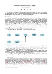
3.1 Springs with no length constraints 

Consider a set Γ of springs with nominal § £ length 

0 

and rigidity coefficient £ positioned one after the other, as 

depicted in Figure 1. Let 0 be the total length of the array, 

that is the sum of the nominal lengths: ¦ 0 

89 £¤£ 1§ £ 0. If

¤ 

¢ 

¢ 

¤ 

¤ 

§ 

¤ 

§ 


x 10 

x 20 

x 30 

x 40 

k 1 k 2 k 3 k 4 

L max 

L 0 

L 

x 1 x 2 x 3 x 4 

k 1 

k 2 

k 3 

k 4 

L’ 

L max 

F 

L 0 

L 

Figure 1. A linear spring system: the total length is 0 when springs are uncompressed (a); and 

0 when springs are compressed (b). 

 

the array is compressed so that its total length is equal to a 

0), the first problem we want 

 

length 5 desired 0 5 (0 

to solve is to find the length§ £ new of each spring, assuming 

that for all , 0 § £ § £ 0. Being 75 the total length of the 

compressed array of springs, we have: 

¡ 

§ £ (1) 

equations (3) and (4) to the set Γ§ of variable springs, we 

have 

where 

¥ £ 2 

£ 

§ £ 

 

§ £ 

0 

 

0 65 

 

¦ 

Γ§ 

¦ £ 

(5) 

§ £¦¡¤£¥ (6) 

5 

 

££ 1 

¢ 

£ Γ © 

If ¢ is the force that keeps a spring in its compressed state, 

then, for the equilibrium of the system, it must be: 

£ ¡ 

¦ £ 

 

§ £ 

0 

§ £ (2) 

 

Solving the equations (1) and (2) for the unknown § 1, § 2, 

, § , we have: 

where 

¡ 

§ £ 

 

§ £ 

£ 

 

0 0 5 

 

 

1 

3.2 Introducing length constraints 

£¤£ 1 1 ¥ 

£ 

¦ 

(3) 

£ 

(4) 

If each spring has a length constraint, in the sense that its 

length cannot be less than a minimum value§ £¢¡¨£¥ , then the 

problem of finding the values § £ requires an iterative solution. 

In fact, if during compression one or more springs 

reach their minimum length, the additional compression 

force will only deform the remaining springs. Thus, at 

each instant, the set Γ can be divided into two subsets: a set 

of fixed springs having minimum length, and a set Γ§ 

Γ¦ 

of variable springs that can still be compressed. Applying 

1 

 

 

£ Γ © 

¥ 1 

£ 

(7) 

Whenever there exists some spring for which equation (5) 

gives § £ § £ ¡¤£¥ , the length of that spring has to be fixed 

at its minimum value, sets Γ¦ and Γ§ must be updated, and 

equations (5), (6) and (7) recomputed for the new set Γ§ . If 

there exists a feasible solution, that is, if the desired final 

length 5 is greater than or equal to the minimum possible 

length of the array * £ 

££ 1§ £¦¡¤£¥ , the iterative 

process ends when each value computed by equations (5) is 

greater than or equal to its corresponding minimum § £¦¡¤£¥ . 

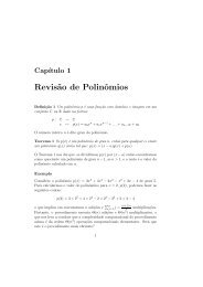
The complete algorithm for compressing a set Γ of springs 

with length constraints up to a desired length -5 is shown 

in Figure 2. 

4. Compressing tasks’ utilizations 

When dealing with a set of elastic tasks, equations (5), 

(6) and (7) can be rewritten by substituting all length parameters 

with the corresponding utilization factors, and the 

rigidity £ coefficients and § with the corresponding elastic 

coefficients ¤ and § . Similarly, at each instant, the set 

£ 

Γ of periodic tasks can be divided into two subsets: a ¦ Γ¦ set 

of fixed tasks having minimum utilization, and Γ§ a set of 

variable tasks that can still be compressed. £ 

 

If ¥ £© ¦ £ 

0 

0 

 

¨¦

£ 

¤ 

£ 

§ 

 

£ 

 

¦ 

 

 

¤ 

 

£ 

 

 

£ 

£ 

¦ 

 

 

£ 

 

 

£ 

¦ 

 

 

 

¦ 

 

£ 


Algorithm Spring compress(Γ, 15 ) 

0 

££ 1§ £ 0; 

* £ £¤£ 1§ £¢¡¤£¢¥ ; 

( 5 * £ if ) return INFEASIBLE; 

do 

Algorithm Task compress(Γ, 5 ) 

 

0 1¥ £ ©¤¦ £ £¤£ 

 

* £ 

9 0; 

£¤£ ¥ £ ©¤¦ £¢¡¨§© 1 

; 

if ( 

do 

5 

* £ ) return INFEASIBLE; 

Γ¦ = ¥ £¢¡§ £ 

 

§ £¦¡¤£¥¤£ ; 

Γ§ 

Γ Γ¦ ; 

§ 

0; 

for ( ¢ £ ) 

if (( £ 

 

0) or (¦ £ 

 

¦ £ ¡ § © )) 

© 

£ Γ § £ ¡¤£¥ ; 

 

£ ; 

1 

¦¥ 

£¨§ Γ 1 ¥ 

£ 

; 

else § 

 

£ ; 

¦ 

© ¦ 

1; 

for ( ¥ £ 2 Γ§ ) 

 

£ 

 

§ £ 

0 

 

0 5 

 

¦ 

§ 

(§ £ § £¦¡¤£¥ if ) 

£ 

 

§ £¢¡¤£¢¥ ; 

© ¦ 

§ 

0; 

§ © ¦ £ ; 

© ¦ 

1; 

for ( ¢ £ 2 Γ§ ) 

if (( 

0) and (¦ £ ¦ £¦¡¨§ © )) £ 

£ 

 

£ 

 

0 

£ 

 

¥ £© 

 

£ ; ¦ 

(¦ £ ¦ £¢¡ § © if ) 

£ 

 

¦ £¦¡¨§ © ; 

© ¦ 

¦ 

0; 

 

0 

5 

 

¦ 

 

£ © § ; 

while ( © ¦ 

0); 

£ 

return FEASIBLE; 

§ 

while ( © ¦ 

0); 

£ 

return FEASIBLE; 

Figure 2. Algorithm for compressing a set of 

springs with length constraints. 

is the nominal utilization of task ¢ £ , 

0 is the sum of all the 

nominal utilizations, and ¦ is the total utilization factor of 

tasks in 

, then to achieve a desired utilization 

5 0 

Γ¦ 

each task has to be compressed up to the following utilization: 

where 

£ 

¢ £ 2 Γ§ 

£ 

 

£ 

 

0 

 

¢ 

£ Γ 

¢ 

£ Γ 

0 

5 

 

¦ 

£ 

 

§ 

(8) 

 

£¢¡¨£¥ (9) 

 

£ (10) 

Figure 3. Algorithm for compressing a set of 

elastic tasks. 

again to the tasks Γ§ in . If there exists a feasible solution, 

that is, if the desired utilization 5 is greater than or equal 

to the minimum possible utilization 

* £ 

££ 

 

£ ¡ § © 1 

, 

the iterative process ends when each value computed by 

equation (8) is greater than or equal to its corresponding 

minimum £ ¡¤£¢¥ . The algorithm 1 for compressing a set Γ 

of 

elastic tasks up to a desired utilization 

5 is shown in 

 

Figure 3. 

4.1 Decompression 

§ 

If there exist tasks for which 

of those tasks has to be fixed at its maximum value ¦ £ ¡ § © 

(so that £ 

 

£¦¡¤£¥ ), sets Γ¦ and Γ§ must be updated 

(hence, ¦ and § recomputed), and equation (8) applied 

 

£ 

£ ¡¤£¢¥ , then the period 

All tasks’ utilizations that have been compressed to cope 

with an overload situation can return toward their nominal 

1 The actual implementation of the algorithm contains more checks on 

tasks’ variables, which are not shown here to simplify its description.

§ 

§ 

§ 

 

 

§ 

¢ 

 

 

 

 

 

£ 

 

 

 

¢ 

£ 

£ 

 

 

 

' 

¥ 

¢ 

 

£ 

 

¡ 

 

£ 

¥ £ ¢ 

£ 

¡ 

 

¦ 

 

¢ 

¢ 

¢ 

¢ 

 

 

 

 

¡ 

 

 

¡ 

 

 

 

 


values when the overload is over. Let Γ be the subset of 

compressed tasks (that is, the set of tasks with ¦ £ ¦ £ 0), 

Γ, let be the set of remaining tasks in Γ (that is, the set of 

be the current processor 

5 

tasks ¦ £ ' ¦ £ with 0), and let 

utilization of Γ. Whenever a task in 

decreases its rate or 

Γ, 

returns to its nominal period, all tasks in Γ can expand their 

utilizations according to their elastic coefficients, so that the 

processor utilization is kept at the value of 5 . 

 

Now, let be the total utilization of Γ , , let be the 

total utilization of , and let 

0 

be the total utilization Γ, of 

tasks in Γ at their nominal periods. It can easily be 

seen 

 

that , ' 

if 

0 

all tasks in Γ can return to their 

nominal periods. On the other 

hand, , 

 

¤ if 

0 

, 

then the release operation of the tasks in Γ can be viewed 

as Γ¦ Γ, a Γ§ 

compression, where and Γ . Hence, it 

can still be performed by using equations (8), (9) and (10) 

and the algorithm presented in Figure 3. 

Lemma 2 In any feasible EDF schedule ¡ , the following 

condition holds: 

£ ¡ 

0 

 

£ 

¡ 

 

1 £¤£ 

' 

 

¢ 

¤£ 

¡ 

 

1 ££ 

¡ £ 

 

 

¥ £ © ¦ £ where , £ 

¡ 

is the remaining execution time of 

£ 

the current instance of at time , and £ 

¡ 

is the next 

task¢ £ 

of¢ £ release time greater than or equal ¡ to t. 

Proof. 

By definition of £ 

¡ 

, we have 

 

£ 

¡ 

 

 

¡ 

5. Theoretical validation of the model 

£ 

¡ 

 

and, by Lemma 1, 

In this section we derive some theoretical results which 

validate the elastic guarantee algorithm that can be performed 

with this method. In particular, we show that if 

tasks’ periods are changed at opportune instants the task set 

remains schedulable and no deadline is missed. The following 

lemmas state two properties of the EDF algorithm that 

are useful for proving the main theorem. 

 

£ 

¡ 

 

1 ££ 

£¤£ 1 

£¤£ 1 

¦ £ 

¦ £ 

¡ 

 

£ 

¥ £ ¢ 

£ 

¡ 

 

' 

¦ 

¡ 

 

£ 

¥ £ ¡ 

£ 

¦ 

Lemma 1 In any feasible EDF schedule ¡ , the following 

condition holds: 

£¤£ 1 

£ 

 

¡ 

¦ £ 

¦ 

£ 

 

£ ¡ 

0 

£¤£ 1 

£ 

££ 1 

£ 

¡ 

 

¢ 

 

¡ 

¤£ 

¡ 

 

where 9 ££ 1 

¥ £ © ¦ £ and ¢ £ 

¡ 

is the cumulative time 

executed by all the instances of task¢ £ up to ¡ . 

Proof. 

If ¡ 

¡ 

 

¤£¦¥ 

¢ ££ 1 

£ 

¡ 

 

 

 

¡ 

 

¨ , we have that 

 

¨© 

££ £ ¥ £ 

 

1 

¡ 

£ 

 

¡ 

The following theorem states a property of decompression: 

if at time all the periods are increased from ¦ £ to 

¦ ) 

¡ 

, then the total utilization factor is decreased from to 

) £ 

 

 

£ ££ 1 

. 

Theorem 1 Given a feasible task set Γ, with total utilization 

factor 1 

 

' 

1, if at time all the periods are 

¡ 

¦ 

££ 

to¦ 

) £ 

 

¦ £ 

 

increased from , then for £ £ all 0, 

¡ 

££ 1 

 

¡ 

 

If ¡ 

¡ 

 

¤£¦¥ 

¨ : 

 

¡ 

1 

1 

1 

1 

¢ £¤£ 1 

£ 

¡ 

 

 

¡ 

 

¡ 

¡ 

¡ 

1 

§ 

¢ £¤£ 1 

£ 

¡ 

 

 

 

 

¡ 

 

1 § 

1 

¡ 

¡ 

 

¡ 

 

 

1 

1 

§ 

£¦¥ 

Moreover, 0 being and 1 1 (because 

the system is feasible), we have that, for all 0, 

§ 

 

. ¡ ¡ 

 

¡ 

 

¡ 

 

¡ 

 

' 

) 

 

where 

¡ 

1 

¡ 

2 is the total processor demand of Γ in ¡ 

1 

¡ 

2 , 

 

¥ 

and ") 

 

£ 

. 

1 £¤£ 

Proof. 

As task periods are increased at time , the new release time 

of task¢ £ is: 

¡ 

 

 

¡ 

 

) 

£ 

¡ 

 

 

¡ 

 

¦ £ 

 

¦ ) 

£ 

¤£

¥ 

 

 

' 

' 

¢ 

¢ 

¢ 

¢ 

¢ 

 

 

 

 

 

 

¢ 

¢ 

 

¢ 

¡ 

¥ £ 

 

£ 

¡ 

¥ £ 

 

¢ 

£ 

 

£ 

 

) 

¥ 

£ 

 

¢ 

 

 

£ 

¢ 

 

 

 

 

' 

 

£ 

 

 

 

 


τ 1 

ν 1 

ν 1 

’ 

ν 

2 

τ 2 

ν ’ 2 

3 

ν 3 

ν ’ 

τ 3 

t 

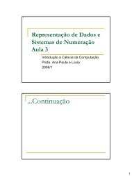
Figure 4. Example of tasks that simultaneously increase their periods at time ¡ . 

The total demand ¡ 

 

¡ 

in is given by the total execution 

time of the instances released after or at with deadlines less 

than or equal to ¡ , plus the remaining execution times 

of the current active instances. The situation considered in 

the proof is illustrated in Figure 4. 

¡ 

Using the result of Lemma 2 we can write: 

 

¡ 

 

¡ 

££ 1 

 

¡ 

 

 

) £ 

¡ 

 

¦ ) 

¡ 

£¤£ 1 

) 

¦ ) 

£ 

¡ 

 

¤£ 

¡ 

 

1 £¤£ 

 

£ 

¡ 

 

1 ££ 

¡ 

 

£ ' 

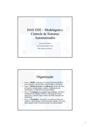
illustrated in Figure 5, where two tasks, ¢ 1 and ¢ 2, with 

computation times 3 and 2, and periods 10 and 3, start at 

29 

time 0. The processor utilization is 30 

, thus the task 

set is schedulable by EDF. At time 14, ¢ 1 changes its 

period 

1 10 to¦ 

) 

1 5. As a consequence, to keep 

from¦ 

the system schedulable, the period ¡ of 2 is increased ¢ from 

2 to¦ 

) 

28 

3 2 6. The new processor utilization is ) ¦ 

so the task set is still feasible; but, if we change the periods 

immediately, task ¢ 1 misses its deadline at time ¡ 15. 

In other words, the period of a compressed task can be 

decreased only at its next release time. Thus, when the QoS 

manager receives a request of period variation, it calculates 

the new periods according to the elastic model: if the new 

30 , 

¢ 

¡ 

 

 

) 

£ 

¡ 

 

1 ££ 

 

) 

1 ££ 

) 

 

£ 

 

£ 

¡ 

 

1 ££ 

 

 

Now, we show that ' 

0. 

£ 

¡ 

 

1 ££ 

£ ) £ 

¡ 

 

¡ 

 

) £ ¡ 

£ 

¡ ) £ 

 

 

it increases the periods of the decompressed tasks immediately, 

but decreases the periods of the compressed tasks 

only at their next release time. Theorem 1 ensures that the 

total processor demand in any interval ¡ 

 

¡ 

exceed 

 

and no deadline will be missed. 

6. Experimental results 

will never 

configuration is found to be feasible (i.e., ) 1), then 

 

) 

£ 

 

£ 

 

Hence, 

¤£ 

¡ 

 

¢ 1 £¤£ 

 

£ 

 

¡ 

 

¦ £ 

¦ ) £ 

) 

£ 

¡ 

 

¦ ) 

 

£ ¡ 

£ 

¡ 

£ ¦ £ 

 

) 

£¤£ ¦ 

£ 

 

¦ £ 

 

) 

£ 

¡ 

 

¦ £ 

¦ ) ¡ 

££ 1 

 

£ 

) 

£ 

¡ 

 

¡ ¦ ) 

£ 1 ¦ £ 

¦ ) £ 

 

' 

0 

1 ££ 

¡ 

 

¡ 

 

' 

) 

 

1 

¦ £ 

¦ ) £ 

 

 

Notice that the property stated by Theorem 1 does not 

hold in case of compression. This can be seen in the example 

The elastic task model has been implemented on top of 

the HARTIK kernel [2, 5], to perform some experiments 

on multimedia applications and verify the results predicted 

by the theory. In particular, the elastic guarantee mechanism 

has been implemented as a high priority task, the QoS 

manager, activated by the other tasks when they are created 

or when they want to change their period. Whenever 

activated, the QoS manager calculates the new periods and 

changes them atomically. According to the result of Theorem 

1, periods are changed at the next release time of the 

task whose period is decreased. If more tasks ask to decrease 

their period, the QoS manager will change them, if 

possible, at their next release time.


τ 1 

τ 2 

0 2 4 6 8 10 12 14 16 18 20 

t 

T = 10 -> 5 

1 

T = 3 -> 6 

Figure 5. A task can miss its deadline if a period is decreased at arbitrary time. 

2 


0 

£¢¡¨£¥ ¦ £¢¡ § © 

¢ 

¢ 

¢ 

1 24 100 30 500 1 

2 24 100 30 500 1 

3 24 100 30 500 1.5 

¢ 4 24 100 30 500 2 

Table 2. Task set parameters used for the first 

experiment. Periods and computation times 

are expressed in milliseconds. 

 

£ 


0 

£¢¡¨£¥ ¦ £¢¡ § © 

¢ 

¢ 

¢ 

¢ 

1 30 100 30 500 1 

2 60 200 30 500 1 

3 90 300 30 500 1 

4 24 50 30 500 1 

Table 3. Task set parameters used for the second 

experiment. Periods and computation 

times are expressed in milliseconds. 

 

£ 

In the first experiment, four periodic tasks are created at 

time 0. Tasks’ parameters are shown in Table 2, while 

the actual number of instances executed by each task as 

a 

function of time is shown in Figure 6. All the tasks start 

executing at their nominal period and, ¡ at 

 

time 1 10 , 

. We recall that a 

¡ 

1 decreases its period to ¦ ) 

1 

¢ 

task cannot decrease its period by itself, but must perform 

a request to the QoS manager, that checks the feasibility of 

the request and calculates the new periods for all the tasks in 

the system. So, at time ¡ 1, since the schedule is found to be 

feasible, the period of¢ 1 is decreased and the periods of¢ 2, 

¢ 3 and¢ 4 are increased according to their elastic coefficients. 

33¡¢ 

 

The values of all the periods are indicated in the graph. 

At time 2 20 

 

, ¢ 1 returns to its nominal period, so 

the QoS manager can change the periods of the other tasks 

to their initial values, as shown in the graph. In this manner, 

the QoS manager ensures that when a task requires to change 

¡ 

its period, the task set remains schedulable and the variation 

of each task period can be controlled by the elastic factor. 

In the second experiment, we tested the elastic model 

as an admission control policy. Three tasks start executing 

at time 0 at their nominal period, while a fourth task 

starts at time 

1 10 

 

. Tasks’ parameters are shown in 

Table 3. When ¡ 4 is started, the task set is not schedulable 

¡ ¢ 

with the current periods, thus the QoS manager, in order 

to accommodate the request of ¢ 4, increases the periods of 

the other tasks according to the elastic model. The actual 

execution rates of the tasks are shown in Figure 7. Notice 

that, although the first three tasks have the same elastic 

coefficients, their periods are changed by a different amount, 

because tasks have different utilization factors. 

7. Conclusions 

In this paper we presented a flexible scheduling theory, in 

which periodic tasks are treated as springs, with given elastic 

coefficients. Under this framework, periodic tasks can 

intentionally change their execution rate to provide different 

quality of service, and the other tasks can automatically 

adapt their periods to keep the system underloaded. The 

proposed model can also be used to handle overload situations 

in a more flexible way. In fact, whenever a new task 

cannot be guaranteed by the system, instead of rejecting the 

task, the system can try to reduce the utilizations of the other 

tasks (by increasing their periods in a controlled fashion) to 

decrease the total load and accommodate the new request. 

As soon as a transient overload condition is over (because


600 

First experiment 

500 

Task 1 




T1=100 ms 

number of executed instances 

400 

300 

200 

T1=33 ms 

T2=100 ms 

T3=100 ms 

T4=100 ms 

100 

T1=T2=T3=T4=100 ms 

T2=175 ms 

T3=277 ms 

T4=500 ms 

0 

0 5000 10000 15000 20000 25000 30000 35000 

t (ms) 

Figure 6. Dynamic period change. 

Second experiment 

200 

T4=50 ms 

number of executed instances 

150 

100 





T1=100 ms 

T1=177 ms 

T2=353 ms 

50 

T2=200 ms 

T3=500 ms 

T3=300 ms 

0 

0 5000 10000 15000 20000 

t (ms) 

Figure 7. Dynamic task activation.


a task terminates or voluntarily increases its period) all the 

compressed tasks may expand up to their original utilization, 

eventually recovering their nominal periods. 

The major advantage of the proposed method is that the 

policy for selecting a solution is implicitly encoded in the 

elastic coefficients provided by the user. Each task is varied 

based on its current elastic status and a feasible configuration 

is found, if there exists one. 

The elastic model is extremely useful for supporting both 

multimedia systems and control applications, in which the 

execution rates of some computational activities have to 

be dynamically tuned as a function of the current system 

state. Furthermore, the elastic mechanism can easily be 

implemented on top of classical real-time kernels,and can be 

used under fixed or dynamic priority scheduling algorithms. 

The experimental results shown in this paper have been 

conducted by implementing the elastic mechanism on the 

HARTIK kernel [2, 5]. 

As a future work, we are investigating the possibility of 

extending this method for dealing with tasks having deadlines 

less than periods, variable execution time, and subject 

to resource constraints. 

References 

[1] T.F. Abdelzaher, E.M. Atkins, and K.G. Shin, “QoS 

Negotiation in Real-Time Systems and Its Applications 

to Automated Flight Control,” Proceedings of the 

IEEE Real-Time Technology and Applications Symposium, 

Montreal, Canada, June 1997. 

[2] G. Buttazzo, “HARTIK: A Real-Time Kernel for 

Robotics Applications”, Proceedings of the 14th IEEE 

Real-Time Systems Symposium, Raleigh-Durham, pp. 

201–205, December 1993. 

[3] M.L. Dertouzos, “Control Robotics: the Procedural 

Control of Physical Processes,” Information Processing, 

74, North-Holland, Publishing Company, 1974. 

[4] T.-W. Kuo and A. K, Mok, “Load Adjustment in Adaptive 

Real-Time Systems,” Proceedings of the 12th 

IEEE Real-Time Systems Symposium, December 1991. 

[5] G. Lamastra, G. Lipari, G. Buttazzo, A. Casile, and F. 

Conticelli, “HARTIK 3.0: A Portable System for Developing 

Real-Time Applications,” Proceedings of the 

IEEE Real-Time Computing Systems and Applications, 

Taipei, Taiwan, October 1997. 

[6] C. Lee, R. Rajkumar, and C. Mercer, “Experiences 

with Processor Reservation and Dynamic QOS in Real- 

Time Mach,” Proceedings of Multimedia Japan 96, 

April 1996. 

[7] C.L. Liu and J.W. Layland, “Scheduling Algorithms 

for Multiprogramming in a Hard real-Time Environment,” 

Journal of the ACM 20(1), 1973, pp. 40–61. 

[8] C. W. Mercer, S. Savage, and H. Tokuda, “Processor 

Capacity Reserves for Multimedia Operating Systems” 

Proceedings of the IEEE International Conference on 

Multimedia Computing and Systems, May 1994. 

[9] A. K. Mok and D. Chen, “A multiframe model for realtime 

tasks,” Proceedings of IEEE Real-Time System 

Symposium, Washington, December 1996. 

[10] T. Nakajima, “Dynamic QOS Control and Resource 

Reservation,” IEICE, RTP’98, 1998. 

[11] T. Nakajima, “Resource Reservation for Adaptive 

QOS Mapping in Real-Time Mach,” Sixth International 

Workshop on Parallel and Distributed Real- 

Time Systems, April 1998. 

[12] T. Nakajima and H. Tezuka, “A Continuous Media Application 

supporting Dynamic QOS Control on Real- 

Time Mach,” Proceedings of the ACM Multimedia ’94, 

1994. 

[13] D. Seto, J.P. Lehoczky, L. Sha, and K.G. Shin, “On 

Task Schedulability in Real-Time Control Systems,” 

Proceedings of the IEEE Real-Time Systems Symposium, 

December 1997. 

[14] M. Spuri, and G.C. Buttazzo, “Efficient Aperiodic Service 

under Earliest Deadline Scheduling”,Proceedings 

of IEEE Real-Time System Symposium, San Juan, Portorico, 

December 1994. 

[15] M. Spuri, G.C. Buttazzo, and F. Sensini, “Robust Aperiodic 

Scheduling under Dynamic Priority Systems”, 

Proceedings of the IEEE Real-Time Systems Symposium, 

Pisa, Italy, December 1995. 

[16] M. Spuri and G.C. Buttazzo, “Scheduling Aperiodic 

Tasks in Dynamic Priority Systems,” Real-Time Systems, 

10(2), 1996. 

[17] J. Sun and J.W.S. Liu, “Bounding Completion Times of 

Jobs with Arbitrary Release Times and Variable Execution 

Times”, Proceedings of IEEE Real-Time System 

Symposium, December 1996. 

[18] T.-S. Tia, Z. Deng, M. Shankar, M. Storch, J. Sun, L.-C. 

Wu, and J.W.-S. Liu, “Probabilistic Performance Guarantee 

for Real-Time Tasks with Varying Computation 

Times,” Proceedings of IEEE Real-Time Technology 

and Applications Symposium, Chicago, Illinois, January 

1995.

Elastic Task Model For Adaptive Rate Control

Create successful ePaper yourself

Delete template?

Save as template?