chapter 1 student notes
chapter 1 student notes
chapter 1 student notes

Create successful ePaper yourself
Turn your PDF publications into a flip-book with our unique Google optimized e-Paper software.
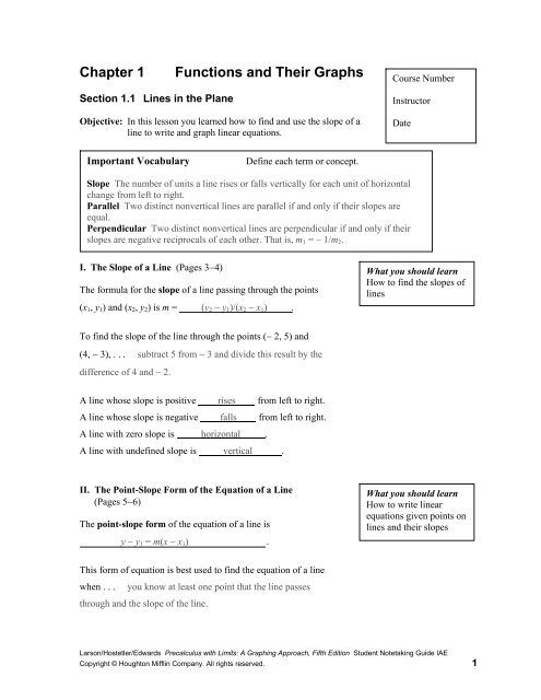
Chapter 1<br />
Functions and Their Graphs<br />
Course Number<br />
Section 1.1 Lines in the Plane<br />
Objective: In this lesson you learned how to find and use the slope of a<br />
line to write and graph linear equations.<br />
Instructor<br />
Date<br />
Important Vocabulary<br />
Define each term or concept.<br />
Slope The number of units a line rises or falls vertically for each unit of horizontal<br />
change from left to right.<br />
Parallel Two distinct nonvertical lines are parallel if and only if their slopes are<br />
equal.<br />
Perpendicular Two distinct nonvertical lines are perpendicular if and only if their<br />
slopes are negative reciprocals of each other. That is, m 1 = – 1/m 2 .<br />
I. The Slope of a Line (Pages 3−4)<br />
The formula for the slope of a line passing through the points<br />
(x 1 , y 1 ) and (x 2 , y 2 ) is m = (y 2 − y 1 )/(x 2 − x 1 ) .<br />
What you should learn<br />
How to find the slopes of<br />
lines<br />
To find the slope of the line through the points (− 2, 5) and<br />
(4, − 3), . . . subtract 5 from − 3 and divide this result by the<br />
difference of 4 and − 2.<br />
A line whose slope is positive rises from left to right.<br />
A line whose slope is negative falls from left to right.<br />
A line with zero slope is horizontal .<br />
A line with undefined slope is vertical .<br />
II. The Point-Slope Form of the Equation of a Line<br />
(Pages 5−6)<br />
The point-slope form of the equation of a line is<br />
y − y 1 = m(x − x 1 ) .<br />
What you should learn<br />
How to write linear<br />
equations given points on<br />
lines and their slopes<br />
This form of equation is best used to find the equation of a line<br />
when . . . you know at least one point that the line passes<br />
through and the slope of the line.<br />
Larson/Hostetler/Edwards Precalculus with Limits: A Graphing Approach, Fifth Edition Student Notetaking Guide IAE<br />
Copyright © Houghton Mifflin Company. All rights reserved. 1
2 Chapter 1 Functions and Their Graphs<br />
The two-point form of the equation of a line is<br />
y − y 1 = (y 2 − y 1 )/(x 2 − x 1 )⋅(x − x 1 ) .<br />
The two-point form of equation is best used to find the equation<br />
of a line when . . . you know the coordinates of two points on<br />
the line.<br />
Example 1: Find an equation of the line having slope − 2 that<br />
passes through the point (1, 5).<br />
y = − 2x + 7<br />
The approximation method used to estimate a point between two<br />
given points is called linear interpolation . The<br />
approximation method used to estimate a point that does not lie<br />
between two given points is called linear extrapolation .<br />
A linear function has the form f(x) = mx + b . Its graph<br />
is a line that has slope m and a y-intercept at<br />
(0, b) .<br />
III. Sketching Graphs of Lines (Pages 7−8)<br />
The slope-intercept form of the equation of a line is<br />
y = mx + b , where m is the slope and the<br />
y-intercept is ( 0 , b ).<br />
What you should learn<br />
How to use slopeintercept<br />
forms of linear<br />
equations to sketch lines<br />
Example 2: Determine the slope and y-intercept of the linear<br />
equation 2 x − y = 4 .<br />
The slope is 2 and the y-intercept is (0, − 4).<br />
The equation of a horizontal line is y = b . The slope of a<br />
horizontal line is 0 . The y-coordinate of every point on the<br />
graph of a horizontal line is b .<br />
The equation of a vertical line is x = a . The slope of a<br />
vertical line is undefined . The x-coordinate of every point<br />
on the graph of a vertical line is a .<br />
The general form of the equation of a line is<br />
Ax + By + C = 0 .<br />
Larson/Hostetler/Edwards Precalculus with Limits: A Graphing Approach, Fifth Edition Student Notetaking Guide IAE<br />
Copyright © Houghton Mifflin Company. All rights reserved.
Section 1.1 Lines in the Plane 3<br />
Every line has an equation that can be written in<br />
form .<br />
general<br />
When a graphing utility is used to sketch a straight line, the<br />
graph of the line may not visually appear to have the slope<br />
indicated by its equation because . . . of the viewing window<br />
used for the graph.<br />
Example 3: Use a graphing utility to graph the linear equation<br />
2 x − y = 4 using (a) a standard viewing window,<br />
and (b) a square window.<br />
(a)<br />
(b)<br />
IV. Parallel and Perpendicular Lines (Pages 9−10)<br />
The relationship between the slopes of two lines that are parallel<br />
is . . . that the slopes are equal.<br />
What you should learn<br />
How to use slope to<br />
identify parallel and<br />
perpendicular lines<br />
The relationship between the slopes of two lines that are<br />
perpendicular is . . . that the slopes are negative reciprocals of<br />
each other.<br />
A line that is parallel to a line whose slope is 2 has slope 2 .<br />
A line that is perpendicular to a line whose slope is 2 has slope<br />
− 1/2 .<br />
What must be done to make the graphs of two perpendicular<br />
lines appear to intersect at right angles when they are graphed<br />
using a graphing utility?<br />
The perpendicular lines must be graphed using a square viewing<br />
window.<br />
Larson/Hostetler/Edwards Precalculus with Limits: A Graphing Approach, Fifth Edition Student Notetaking Guide IAE<br />
Copyright © Houghton Mifflin Company. All rights reserved.
4 Chapter 1 Functions and Their Graphs<br />
Example 4: Use a graphing utility to graph the perpendicular<br />
lines y = 2x<br />
− 3 and y = −0 .5x<br />
+ 5 using (a) a<br />
standard viewing window, and (b) a square<br />
window.<br />
(a)<br />
(b)<br />
Additional <strong>notes</strong><br />
y<br />
y<br />
y<br />
x<br />
x<br />
x<br />
Homework Assignment<br />
Page(s)<br />
Exercises<br />
Larson/Hostetler/Edwards Precalculus with Limits: A Graphing Approach, Fifth Edition Student Notetaking Guide IAE<br />
Copyright © Houghton Mifflin Company. All rights reserved.
Section 1.2 Functions 5<br />
Section 1.2 Functions<br />
Objective: In this lesson you learned how to evaluate functions and find<br />
their domains.<br />
Course Number<br />
Instructor<br />
Date<br />
Important Vocabulary<br />
Define each term or concept.<br />
Function A function f from a set A to a set B is a relation that assigns to each element<br />
x in the set A exactly one element y in the set B.<br />
Domain The set of inputs of the function f.<br />
Range The set of all outputs for the given set of inputs of the function f.<br />
Independent variable A variable in an equation that represents a function that can<br />
take on any value for which the function is defined.<br />
Dependent variable A variable in an equation that represents a function whose value<br />
depends on the value of the independent variable.<br />
I. Introduction to Functions (Pages 16−18)<br />
A rule of correspondence that matches quantities from one set<br />
with items from a different set is a relation .<br />
What you should learn<br />
How to decide whether a<br />
relation between two<br />
variables represents a<br />
function<br />
In functions that can be represented by ordered pairs, the first<br />
coordinate in each ordered pair is the input and the<br />
second coordinate is the output .<br />
Some characteristics of a function from Set A to Set B are . . .<br />
1) Each element of A must be matched with an element<br />
of B.<br />
2) Some elements of B may not be matched with any<br />
element of A.<br />
3) Two or more elements of A may be matched with the<br />
same element of B.<br />
4) An element of A (the domain) cannot be matched with<br />
two different elements of B.<br />
To determine whether or not a relation is a function, . . .<br />
decide whether each input value is matched with exactly one<br />
output value.<br />
Larson/Hostetler/Edwards Precalculus with Limits: A Graphing Approach, Fifth Edition Student Notetaking Guide IAE<br />
Copyright © Houghton Mifflin Company. All rights reserved.
6 Chapter 1 Functions and Their Graphs<br />
If any input value of a relation is matched with two or more<br />
output values, . . . the relation is not a function.<br />
Some common ways to represent functions are . . .<br />
1) Verbally in a sentence<br />
2) Numerically in a table or list of ordered pairs<br />
3) Graphically by points on a graph in the coordinate plane<br />
4) Algebraically by an equation in two variables<br />
Example 1: Decide whether the table represents y as a function<br />
of x.<br />
x − 3 − 1 0 2 4<br />
y 5 − 12 5 3 14<br />
Yes, this table represents y as a function of x.<br />
II. Function Notation (Pages 18−20)<br />
The symbol f(x) is function notation for the value<br />
of f at x or simply f of x. The symbol f(x) corresponds to the<br />
y-value for a given x.<br />
Keep in mind that f is the name of the function,<br />
whereas f(x) is the output value of the function at the<br />
input value x.<br />
What you should learn<br />
How to use function<br />
notation and evaluate<br />
functions<br />
In function notation, the input is the independent<br />
variable and the output is the dependent variable.<br />
3<br />
Example 2: If f ( w)<br />
= 4w<br />
− 5w<br />
− 7w<br />
+ 13 , describe how to<br />
find f (−2)<br />
.<br />
Replace each occurrence of w in the function by<br />
− 2 and evaluate the resulting numerical<br />
expression.<br />
A piecewise-defined function is . . . a function that is defined<br />
by two or more equations over a specified domain.<br />
2<br />
Larson/Hostetler/Edwards Precalculus with Limits: A Graphing Approach, Fifth Edition Student Notetaking Guide IAE<br />
Copyright © Houghton Mifflin Company. All rights reserved.
Section 1.2 Functions 7<br />
III. The Domain of a Function (Page 20−21)<br />
The implied domain of a function defined by an algebraic<br />
expression is . . . the set of all real numbers for which the<br />
expression is defined.<br />
What you should learn<br />
How to find the domains<br />
of functions<br />
In general, the domain of a function excludes values that . . .<br />
would cause division by zero or result in the even root of a<br />
negative number.<br />
For example, the implied domain of the function f ( x)<br />
= 5x<br />
− 8<br />
is . . . the set of all real numbers greater than or equal to 8/5, or<br />
[8/5, ∞).<br />
IV. Applications of Functions (Page 22)<br />
Example 3: The price P (in dollars) of a child’s handmade<br />
sweater is given by the function P(s) = 3s + 15,<br />
where s represents the size (size 1, size 2, etc.) of<br />
the sweater. Use this function to find the price of a<br />
child’s size 5 handmade sweater.<br />
$30<br />
What you should learn<br />
How to use functions to<br />
model and solve real-life<br />
problems<br />
V. Difference Quotients (Page 23)<br />
A difference quotient is defined as . . .<br />
[f(x + h) − f(x)]/h, h ≠ 0.<br />
What you should learn<br />
How to evaluate<br />
difference quotients<br />
Describe a real-life situation which can be represented by a<br />
function.<br />
Answers will vary.<br />
Additional <strong>notes</strong><br />
Larson/Hostetler/Edwards Precalculus with Limits: A Graphing Approach, Fifth Edition Student Notetaking Guide IAE<br />
Copyright © Houghton Mifflin Company. All rights reserved.
8 Chapter 1 Functions and Their Graphs<br />
Additional <strong>notes</strong><br />
y<br />
y<br />
y<br />
x<br />
x<br />
x<br />
y<br />
y<br />
y<br />
x<br />
x<br />
x<br />
Homework Assignment<br />
Page(s)<br />
Exercises<br />
Larson/Hostetler/Edwards Precalculus with Limits: A Graphing Approach, Fifth Edition Student Notetaking Guide IAE<br />
Copyright © Houghton Mifflin Company. All rights reserved.
Section 1.3 Graphs of Functions 9<br />
Section 1.3 Graphs of Functions<br />
Objective: In this lesson you learned how to analyze the graphs of<br />
functions.<br />
Course Number<br />
Instructor<br />
Date<br />
Important Vocabulary<br />
Define each term or concept.<br />
Graph of a function The collection of ordered pairs (x, f(x)) such that x is in the<br />
domain of f.<br />
Greatest integer function The greatest integer function is denoted by [|x|] and is<br />
defined as the greatest integer less than or equal to x.<br />
Step function A function whose graph resembles a set of stair steps.<br />
Even function A function whose graph is symmetric with respect to the y-axis.<br />
Odd function A whose graph is symmetric with respect to the origin.<br />
I. The Graph of a Function (Pages 30−31)<br />
Explain the use of open or closed dots in the graphs of functions.<br />
The use of dots, open or closed, at the extreme left or right points<br />
of a graph indicates that the graph does not extend beyond these<br />
points. If no such dots are shown, assume that the graph extends<br />
beyond these points.<br />
What you should learn<br />
How to find the domains<br />
and ranges of functions<br />
and how to use the<br />
Vertical Line Test for<br />
functions<br />
To find the domain of a function from its graph, . . . examine<br />
the graph to see for which x-values the graph is plotted.<br />
To find the range of a function from its graph, . . .<br />
graph to see for which y-values the graph is plotted.<br />
examine the<br />
The Vertical Line Test for functions states . . . that a set of<br />
points in a coordinate plane is the graph of y as a function of x if<br />
and only if no vertical line intersects the graph at more than one<br />
point.<br />
Larson/Hostetler/Edwards Precalculus with Limits: A Graphing Approach, Fifth Edition Student Notetaking Guide IAE<br />
Copyright © Houghton Mifflin Company. All rights reserved.
10 Chapter 1 Functions and Their Graphs<br />
Example 1: Decide whether each graph represents y as a<br />
function of x.<br />
(a)<br />
(b)<br />
(a) Yes, this is a graph of y as a<br />
function of x<br />
(b) No, this is not a graph of y as<br />
a function of x<br />
II. Increasing and Decreasing Functions (Page 32)<br />
A function f is increasing on an interval if, for any x 1 and x 2 in<br />
the interval, . . . x 1 < x 2 implies f(x 1 ) < f(x 2 ).<br />
A function f is decreasing on an interval if, for any x 1 and x 2 in<br />
the interval, . . . x 1 < x 2 implies f(x 1 ) > f(x 2 ).<br />
A function f is constant on an interval if, for any x 1 and x 2 in the<br />
interval,. . . f(x 1 ) = f(x 2 ).<br />
What you should learn<br />
How to determine<br />
intervals on which<br />
functions are increasing,<br />
decreasing, or constant<br />
Given a graph of a function, to find an interval on which the<br />
function is increasing . . . search for an interval over which<br />
the graph rises from left to right.<br />
Given a graph of a function, to find an interval on which the<br />
function is decreasing . . . search for an interval over which<br />
the graph falls from left to right.<br />
Given a graph of a function, to find an interval on which the<br />
function is constant . . . search for an interval over which the<br />
graph is level.<br />
III. Relative Minimum and Maximum Values<br />
(Pages 33−34)<br />
A function value f(a) is called a relative minimum of f if . . .<br />
there exists an interval (x 1 , x 2 ) that contains a such that<br />
x 1 < x < x 2 implies f(a) ≤ f(x).<br />
What you should learn<br />
How to determine<br />
relative maximum and<br />
relative minimum values<br />
of functions<br />
Larson/Hostetler/Edwards Precalculus with Limits: A Graphing Approach, Fifth Edition Student Notetaking Guide IAE<br />
Copyright © Houghton Mifflin Company. All rights reserved.
Section 1.3 Graphs of Functions 11<br />
A function value f(a) is called a relative maximum of f if . . .<br />
there exists an interval (x 1 , x 2 ) that contains a such that<br />
x 1 < x < x 2 implies f(a) ≥ f(x).<br />
The point at which a function changes from increasing to<br />
decreasing is a relative maximum . The point at which<br />
a function changes from decreasing to increasing is a relative<br />
minimum .<br />
To approximate the relative minimum or maximum of a function<br />
using a graphing utility, . . . use the zoom and trace features to<br />
approximate the lowest or highest point on the graph, OR use a<br />
built-in program or feature for finding minimum or maximum<br />
values.<br />
Example 2: Suppose a function C represents the annual<br />
number of cases (in millions) of chicken pox<br />
reported for the year x in the United States from<br />
1960 through 2000. Interpret the meaning of the<br />
function’s minimum at (1998, 3).<br />
The lowest number of cases of chicken pox reported<br />
during this period was 3 million cases in 1998.<br />
IV. Graphing Step Functions and Piecewise-Defined<br />
Functions (Page 35)<br />
Describe the graph of the greatest integer function.<br />
The graph of the greatest integer function jumps vertically one<br />
unit at each integer and is constant (a horizontal line segment)<br />
between each pair of consecutive integers.<br />
What you should learn<br />
How to identify and<br />
graph step functions and<br />
other piecewise-defined<br />
functions<br />
Example 3: Let<br />
f ( x)<br />
= x , the greatest integer function. Find<br />
f (3.74) .<br />
3<br />
To sketch the graph of a piecewise-defined function, . . .<br />
sketch the graph of each equation of the piecewise-defined<br />
function over the appropriate portion of the domain.<br />
Larson/Hostetler/Edwards Precalculus with Limits: A Graphing Approach, Fifth Edition Student Notetaking Guide IAE<br />
Copyright © Houghton Mifflin Company. All rights reserved.
12 Chapter 1 Functions and Their Graphs<br />
V. Even and Odd Functions (Pages 36−37)<br />
A graph is symmetric with respect to the y-axis if, whenever<br />
(x, y) is on the graph, (− x, y) is also on the graph. A graph<br />
is symmetric with respect to the x-axis if, whenever (x, y) is on<br />
the graph, (x, − y) is also on the graph. A graph is<br />
symmetric with respect to the origin if, whenever (x, y) is on the<br />
graph, (− x, − y) is also on the graph. A graph that is<br />
symmetric with respect to the x-axis is . . .<br />
not the graph of a function (except for the graph of y = 0).<br />
What you should learn<br />
How to identify even and<br />
odd functions<br />
A function f is even if, for each x in the domain of f,<br />
f(−x) = f(x) .<br />
A function f is even if, for each x in the domain of f,<br />
f(−x) = f(x) .<br />
Additional <strong>notes</strong><br />
y<br />
y<br />
y<br />
x<br />
x<br />
x<br />
Homework Assignment<br />
Page(s)<br />
Exercises<br />
Larson/Hostetler/Edwards Precalculus with Limits: A Graphing Approach, Fifth Edition Student Notetaking Guide IAE<br />
Copyright © Houghton Mifflin Company. All rights reserved.
Section 1.4 Shifting, Reflecting, and Stretching Graphs 13<br />
Section 1.4 Shifting, Reflecting, and Stretching Graphs<br />
Objective: In this lesson you learned how to identify and graph shifts,<br />
reflections, and nonrigid transformations of functions.<br />
Course Number<br />
Instructor<br />
Date<br />
Important Vocabulary<br />
Define each term or concept.<br />
Vertical shift A transformation of the graph of y = f(x), represented by h(x) = f(x) ± c,<br />
in which the graph is shifted upward or downward c units respectively (c is a positive<br />
real number).<br />
Horizontal shift A transformation of the graph of y = f(x), represented by<br />
h(x) = f(x ± c), in which the graph is shifted to the left or to the right c units<br />
respectively (c is a positive real number).<br />
Rigid transformations Transformations in which the basic shape of the graph is<br />
unchanged.<br />
Nonrigid transformations Transformations that cause a distortion (a change in the<br />
original shape of the graph).<br />
I. Summary of Graphs of Parent Functions (Page 42)<br />
Sketch an example of each of the six most commonly used<br />
functions in algebra.<br />
What you should learn<br />
How to recognize graphs<br />
of parent functions<br />
Constant Function<br />
y<br />
Identity Function<br />
y<br />
x<br />
x<br />
Absolute Value Function<br />
y<br />
Square Root Function<br />
y<br />
x<br />
x<br />
Larson/Hostetler/Edwards Precalculus with Limits: A Graphing Approach, Fifth Edition Student Notetaking Guide IAE<br />
Copyright © Houghton Mifflin Company. All rights reserved.
14 Chapter 1 Functions and Their Graphs<br />
Quadratic Function<br />
y<br />
Cubic Function<br />
y<br />
x<br />
x<br />
II. Vertical and Horizontal Shifts (Pages 43−44)<br />
Let c be a positive real number. Complete the following<br />
representations of shifts in the graph of y = f (x)<br />
:<br />
1) Vertical shift c units upward: h(x) = f(x) + c<br />
2) Vertical shift c units downward: h(x) = f(x) − c<br />
3) Horizontal shift c units to the right: h(x) = f(x − c)<br />
4) Horizontal shift c units to the left: h(x) = f(x + c)<br />
What you should learn<br />
How to use vertical and<br />
horizontal shifts and<br />
reflections to graph<br />
functions<br />
Example 1: Let f ( x)<br />
= x . Write the equation for the<br />
function resulting from a vertical shift of 3 units<br />
downward and a horizontal shift of 2 units to the<br />
right of the graph of f (x)<br />
.<br />
f(x) = | x − 2 | − 3<br />
III. Reflecting Graphs (Pages 45−46)<br />
A reflection in the x-axis is a type of transformation of the graph<br />
of y = f(x) represented by h(x) = − f(x) . A reflection in<br />
the y-axis is a type of transformation of the graph of y = f(x)<br />
represented by h(x) = f(− x) .<br />
Example 2: Let f ( x)<br />
= x . Describe the graph of g(<br />
x)<br />
= − x<br />
in terms of f .<br />
The graph of g is a reflection of the graph of f in<br />
the x-axis.<br />
Larson/Hostetler/Edwards Precalculus with Limits: A Graphing Approach, Fifth Edition Student Notetaking Guide IAE<br />
Copyright © Houghton Mifflin Company. All rights reserved.
Section 1.4 Shifting, Reflecting, and Stretching Graphs 15<br />
IV. Nonrigid Transformations (Page 47)<br />
Name three types of rigid transformations:<br />
1) Horizontal shifts<br />
2) Vertical shifts<br />
3) Reflections<br />
What you should learn<br />
How to use nonrigid<br />
transformations to graph<br />
functions<br />
Rigid transformations change only the position of the<br />
graph in the coordinate plane.<br />
Name four types of nonrigid transformations:<br />
1) Vertical stretch<br />
2) Vertical shrink<br />
3) Horizontal shrink<br />
4) Horizontal stretch<br />
A nonrigid transformation y = cf (x)<br />
of the graph of y = f (x)<br />
is<br />
a vertical stretch if c > 1 or a vertical shrink if<br />
0 < c < 1. A nonrigid transformation y= f( cx)<br />
of the graph of<br />
y = f (x) is a horizontal shrink if c > 1 or a<br />
horizontal stretch if 0 < c < 1.<br />
Additional <strong>notes</strong><br />
y<br />
y<br />
y<br />
x<br />
x<br />
x<br />
Larson/Hostetler/Edwards Precalculus with Limits: A Graphing Approach, Fifth Edition Student Notetaking Guide IAE<br />
Copyright © Houghton Mifflin Company. All rights reserved.
16 Chapter 1 Functions and Their Graphs<br />
Additional <strong>notes</strong><br />
y<br />
y<br />
y<br />
x<br />
x<br />
x<br />
y<br />
y<br />
y<br />
x<br />
x<br />
x<br />
Homework Assignment<br />
Page(s)<br />
Exercises<br />
Larson/Hostetler/Edwards Precalculus with Limits: A Graphing Approach, Fifth Edition Student Notetaking Guide IAE<br />
Copyright © Houghton Mifflin Company. All rights reserved.
Section 1.5 Combinations of Functions 17<br />
Section 1.5 Combinations of Functions<br />
Objective: In this lesson you learned how to find arithmetic<br />
combinations and compositions of functions.<br />
Course Number<br />
Instructor<br />
Date<br />
I. Arithmetic Combinations of Functions (Pages 51−53)<br />
Just as two real numbers can be combined by the operations of<br />
addition, subtraction, multiplication, and division to form other<br />
real numbers, two functions f and g can be combined to create<br />
new functions such as the sum, difference, product, and<br />
quotient<br />
of f and g to create new functions.<br />
What you should learn<br />
How to add, subtract,<br />
multiply, and divide<br />
functions<br />
The domain of an arithmetic combination of functions f and g<br />
consists of . . . all real numbers that are common to the<br />
domains of f and g. In the case of the quotient f(x)/g(x), there is<br />
the further restriction that g(x) ≠ 0.<br />
Let f and g be two functions with overlapping domains.<br />
Complete the following arithmetic combinations of f and g for all<br />
x common to both domains:<br />
1) Sum: ( f + g)(<br />
x)<br />
= f(x) + g(x)<br />
2) Difference: ( f − g)(<br />
x)<br />
= f(x) − g(x)<br />
3) Product: ( fg )( x)<br />
= f(x) · g(x)<br />
⎛ f ⎞<br />
4) Quotient: ⎜<br />
⎟(x)<br />
=<br />
⎝ g ⎠<br />
f(x) ÷ g(x), g(x) ≠ 0<br />
To use a graphing utility to graph the sum of two functions, . . .<br />
enter the first function as y 1 and enter the second function as y 2 .<br />
Define y 3 as y 1 + y 2 , then graph y 3 .<br />
Example 1: Let f ( x)<br />
= 7x<br />
− 5 and g( x)<br />
= 3 − 2x<br />
. Find<br />
( f − g)(4) .<br />
28<br />
Larson/Hostetler/Edwards Precalculus with Limits: A Graphing Approach, Fifth Edition Student Notetaking Guide IAE<br />
Copyright © Houghton Mifflin Company. All rights reserved.
18 Chapter 1 Functions and Their Graphs<br />
II. Compositions of Functions (Pages 53−56)<br />
The composition of the function f with the function g is<br />
( f g)( x ) = f(g(x)) .<br />
What you should learn<br />
How to find<br />
compositions of one<br />
function with another<br />
function<br />
For the composition of the function f with g, the domain of<br />
f g is . . . the set of all x in the domain of g such that<br />
g(x) is in the domain of f.<br />
Example 2: Let f ( x)<br />
= 3x<br />
+ 4 and let g ( x)<br />
= 2x 2 −1. Find<br />
(a) ( f g)(<br />
x)<br />
and (b) ( g f )( x)<br />
.<br />
(a) 6x 2 + 1 (b) 18x 2 + 48x + 31<br />
III. Applications of Combinations of Functions (Page 57)<br />
The function f ( x)<br />
= 0. 06x<br />
represents the sales tax owed on a<br />
purchase with a price tag of x dollars and the function<br />
g( x)<br />
= 0. 75x<br />
represents the sale price of an item with a price tag<br />
of x dollars during a 25% off sale. Using one of the combinations<br />
of functions discussed in this section, write the function that<br />
represents the sales tax owed on an item with a price tag of x<br />
dollars during a 25% off sale.<br />
What you should learn<br />
How to use combinations<br />
of functions to model and<br />
solve real-life problems<br />
(f g)(x) = (g f)(x) = 0.045x<br />
Additional <strong>notes</strong><br />
Homework Assignment<br />
Page(s)<br />
Exercises<br />
Larson/Hostetler/Edwards Precalculus with Limits: A Graphing Approach, Fifth Edition Student Notetaking Guide IAE<br />
Copyright © Houghton Mifflin Company. All rights reserved.
Section 1.6 Inverse Functions 19<br />
Section 1.6 Inverse Functions<br />
Objective: In this lesson you learned how to find inverse functions<br />
graphically and algebraically.<br />
Course Number<br />
Instructor<br />
Date<br />
Important Vocabulary<br />
Define each term or concept.<br />
Inverse function Let f and g be two functions. If f(g(x)) = x for every x in the domain<br />
of g and g(f(x)) = x for every x in the domain of f, then g is the inverse function of the<br />
function f. The function g is denoted by f −1 .<br />
One-to-one A function f is one-to-one if, for a and b in its domain, f(a) = f(b) implies<br />
a = b.<br />
Horizontal Line Test A function is one-to-one if every horizontal line intersects the<br />
graph of the function at most once.<br />
I. Inverse Functions (Pages 62−64)<br />
For a function f that is defined by a set of ordered pairs, to form<br />
the inverse function of f, . . . interchange the first and second<br />
coordinates of each of these ordered pairs.<br />
What you should learn<br />
How to find inverse<br />
functions informally and<br />
verify that two functions<br />
are inverse functions of<br />
each other<br />
For a function f and its inverse f −1 , the domain of f is equal to<br />
the range of f −1 , and the range of f is equal to<br />
the domain of f −1 .<br />
To verify that two functions, f and g, are inverses of each other,<br />
. . . find f(g(x)) and g(f(x)). If both of these compositions are<br />
equal to the identity function, then the functions are inverses of<br />
each other.<br />
Example 1: Verify that the functions f ( x)<br />
= 2x<br />
− 3 and<br />
+ 3<br />
g ( x)<br />
= x are inverses of each other.<br />
2<br />
II. The Graph of an Inverse Function (Page 65)<br />
If the point (a, b) lies on the graph of f, then the point<br />
( b , a ) lies on the graph of f −1 and vice versa. The<br />
graph of f −1 is a reflection of the graph of f in the line<br />
y = x .<br />
What you should learn<br />
How to use graphs of<br />
functions to decide<br />
whether functions have<br />
inverse functions<br />
Larson/Hostetler/Edwards Precalculus with Limits: A Graphing Approach, Fifth Edition Student Notetaking Guide IAE<br />
Copyright © Houghton Mifflin Company. All rights reserved.
20 Chapter 1 Functions and Their Graphs<br />
III. The Existence of an Inverse Function (Page 66)<br />
If a function is one-to-one, that means . . . that no two<br />
elements in the domain of the function correspond to the same<br />
What you should learn<br />
How to determine if<br />
functions are one-to-one<br />
element in the range of the function.<br />
A function f has an inverse f −1 if and only if . . .<br />
f is one-to-one.<br />
To tell whether a function is one-to-one from its graph, . . .<br />
simply use the Horizontal Line Test, that is, check to see that<br />
every horizontal line intersects the graph of the function at most once.<br />
Example 2:<br />
Does the graph of the function at the right have an<br />
inverse function? Explain.<br />
No, it doesn’t pass the Horizontal Line Test.<br />
IV. Finding Inverse Functions Algebraically (Pages 67−68)<br />
To find the inverse of a function f algebraically, . . .<br />
1) Use the Horizontal Line Test to decide whether f has an<br />
What you should learn<br />
How to find inverse<br />
functions algebraically<br />
inverse function.<br />
2) In the equation for f(x), replace f(x) by y.<br />
3) Interchange the roles of x and y, and solve for y.<br />
4) Replace y by f −1 (x) in the new equation.<br />
5) Verify that f and f −1 are inverse functions of each other by showing<br />
that the domain of f is equal to the range of f −1 , the range of f is equal<br />
to the domain of f −1 , and f(f −1 (x)) = x and f −1 (f(x)) = x.<br />
Example 3: Find the inverse (if it exists) of f ( x)<br />
= 4x<br />
− 5 .<br />
f −1 (x) = 0.25x + 1.25<br />
Homework Assignment<br />
Page(s)<br />
Exercises<br />
Larson/Hostetler/Edwards Precalculus with Limits: A Graphing Approach, Fifth Edition Student Notetaking Guide IAE<br />
Copyright © Houghton Mifflin Company. All rights reserved.
Section 1.7 Linear Models and Scatter Plots 21<br />
Section 1.7 Linear Models and Scatter Plots<br />
Objective: In this lesson you learned how to use scatter plots and a<br />
graphing utility to find linear models for data.<br />
Course Number<br />
Instructor<br />
Date<br />
Important Vocabulary<br />
Define each term or concept.<br />
Fitting a line to data The process of finding a linear model to represent the<br />
relationship described by a scatter plot.<br />
I. Scatter Plots and Correlation (Pages 73−74)<br />
Many real-life situations involve finding relationships between<br />
two variables. If data is collected and written as a set of ordered<br />
pairs, the graph of such a set is called a scatter plot .<br />
What you should learn<br />
How to construct scatter<br />
plots and interpret<br />
correlation<br />
For a collection of ordered pairs of the form (x, y), if y tends to<br />
increase as x increases, the collection is said to have a(n)<br />
positive correlation . If y tends to decrease as x<br />
increases, the collection is said to have a(n) negative<br />
correlation .<br />
II. Fitting a Line to Data (Pages 74−77)<br />
To fit a line to data represented in a scatter plot, . . . sketch<br />
the line that appears to fit the points, find two points on the line,<br />
and then find the equation of the line that passes through the two<br />
points, OR use the linear regression feature of a graphing utility<br />
to find the linear model.<br />
What you should learn<br />
How to use scatter plots<br />
and a graphing utility to<br />
find linear models for<br />
data<br />
To measure how well a linear model fits the data used to find the<br />
model, . . . compare the actual values with the values given<br />
by the model.<br />
Larson/Hostetler/Edwards Precalculus with Limits: A Graphing Approach, Fifth Edition Student Notetaking Guide IAE<br />
Copyright © Houghton Mifflin Company. All rights reserved.
22 Chapter 1 Functions and Their Graphs<br />
The correlation coefficient r of a set of data varies between<br />
− 1 and 1 . The closer | r | is to 1, the better . . .<br />
the points can be described by a line.<br />
Example 1: The numbers of U.S. Navy personnel p in<br />
thousands on active duty for the years 2002<br />
through 2006 are shown in the table. Use the<br />
regression capabilities of a graphing utility to find<br />
a linear model for the data. Let t represent the year<br />
with t = 2 corresponding to 2002.<br />
Year 2002 2003 2004 2005 2006<br />
p 383 381 376 364 353<br />
(Source: U.S. Department of Defense)<br />
p = − 7.7t + 402.2<br />
y<br />
y<br />
y<br />
x<br />
x<br />
x<br />
y<br />
y<br />
y<br />
x<br />
x<br />
x<br />
Homework Assignment<br />
Page(s)<br />
Exercises<br />
Larson/Hostetler/Edwards Precalculus with Limits: A Graphing Approach, Fifth Edition Student Notetaking Guide IAE<br />
Copyright © Houghton Mifflin Company. All rights reserved.