Spectral characteristics of semiconductor lasers (SPEK)

Chapter 13
Spectral characteristics of semiconductor
lasers (SPEK)
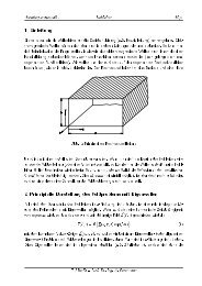
In this chapter we discuss the spectral characteristics of semiconductor lasers.
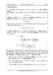
The spectra of index- and gain-guided lasers (compare with chapter HL-STRUK) might be different under
certain circumstances, as shown in Fig. 13.1.
Figure 13.1: (a) index-guided laser, (b) gain-guided laser
If spontaneous emission is neglected, the gain g of the laser is given, according to chapter HL, as:
g = α s − 1
2L · ln(R 1 · R 2 ) (13.1)
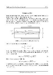
In general, the gain g depends on the wavelength (see Fig. 13.2).
Below the threshold, g increases with an increasing charge carrier density, until, for a given wavelength
λ = λ m , the oscillation build-up condition is achieved.
If spontaneous emission is neglected, only one laser mode (λ m ) resonates at the laser threshold.
Above threshold, the gain remains constant g = g s at the wavelength λ m , i.e. the gain saturates at g = g s .
Two possibilities follow:
1

C
!
C
Introduction to fiber optic communications ONT/ 2
D C A A 5 J J E C K C
E D C A A 5 J J E C K C
C I
!
Figure 13.2: The gain g over the wavlength λ, λ m±i - Resonance wavelength of the laser cavity, curve 1:
homogeneous saturation, curve 2: inhomogeneous saturation
1. Homogeneous saturation of the gain, i.e. the gain g(λ) persits even above the threshold, hence for
only one wavelength λ m the gain g = g s is achieved (curve 1 in Fig. 13.2).
2. Inhomogeneous saturation, i.e. the gain g(λ) increases with increasing injection and is forced to
g = g s at the emission wavelength. This is known as spectral hole-burning (curve 2 in Fig. 13.2).
Homogeneous saturation dominates in a semiconductor laser, since equilibrium within the conduction and
valence band is achieved very fast (time constant ∼ 10 −13 s). For this reason, the spectrum is examined,
assuming a homogeneous line broadening with consideration of the spontaneous emission. The starting
point is the Equation
dS
dt = r st · S − S
τ ph
+ r sp · K (13.2)
from chapter MOD. K (with K ≥ 1 ) is an additional correction factor for the spontaneous emission in
gain-guided lasers. Assuming steady state condition ( d dt = 0 ) the number of photons S(λ µ) within a laser
oscillation at the emission wavelength λ µ :
Using the normalized gain coefficient
r st · S(λ µ ) − S(λ µ)
τ ph
+ r sp · K = 0. (13.3)
G(λ) = r st · τ ph = g g s
(13.4)
and n sp = r sp /r st , Eq. 13.3 is solved to:
S(λ µ ) = n sp · K ·
1
1 − G(λ µ )
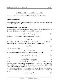
The normalized gain G(λ µ ) coefficient can be approximated by a parabolic curve (see Fig. 13.3):
(
) )
G(λ µ ) = G 0
(1 − 2 · λµ − λ 2
m
∆Λ
(13.5)
(13.6)

Introduction to fiber optic communications ONT/ 3
/
/
,
Figure 13.3: The parabolic approximation of the normalized gain G(λ)
with G 0 = G(λ m ) . Since 1 − G 0 ≪ 1 applies, Eq. 13.6 can be written as:
(
)
G(λ µ ) ≈ G 0 − 2 · λµ − λ 2
m
(13.7)
∆Λ
Therefore the photon number S(λ µ ) is given in the form:
S(λ µ ) ≈
n sp · K
( )
1 − G 0 + 2 · λµ−λ 2
(13.8)
m
∆Λ
and, respectively, the emitted power is (compare with chapter MOD)
P (λ µ ) = K · n sp · h · ν · c (
N −
1
2L ln(R 1R 2 ) )
( )
1 − G 0 + 2 · λµ−λ 2
(13.9)
m
∆Λ
The full width at half maximum (FWHM) δλ of the spectrum can be determined using Eq. (13.9) as:
δλ = ∆Λ √ 1 − G 0 (13.10)
The full width at half maximum δλ can be expressed as a function of the total emitted power P as:
P = ∑ µ
P (λ µ ) (13.11)
and the mode distance (resonance distance) (see chapter HL) as:
Assuming δλ ≫ ∆λ in Eq. (13.9), one obtains:
δλ = c · π · h · ν
2P
∆λ =
· ln
λ2
2N · L . (13.12)
( 1
R 1 R 2
)
n sp · K
( ) ∆Λ 2
(13.13)
λ

Introduction to fiber optic communications ONT/ 4
2
@
,
!
!
Figure 13.4: Lorentzian-shaped spectrum
Example: R 1 = R 2 = 0.32 , n sp = 2.5 , ∆Λ = 30 nm , λ = 850 nm and the power per mirror of
P
2
= 5 mW . Applying these values a FWHM of the spectrum can be determined to δλ = K · 0.08 nm.
The FWHM can be determined for a gain-guided laser with assuming K = 20 to δλ = 1.6 nm .
In an index-guided laser ( K = 1 ) the FWHM is smaller than the distance between the resonance wavelengths
( δλ < ∆λ ), resulting in a single-mode emission. Hence, the different characteristic in Fig. 13.1 is
explained.
Although for an index-guided laser ( K = 1 ), due to Fig. 13.1, a single-mode operation for Fabry-Perot-
Laser is possible, the single-mode emission is not very stable. The emission may be strongly affected by
external reflections or by modulation of the laser (e.g. mode hopping or dynamic multi-mode emission).
A stable single-mode emission can be achieved, if the reflectors R 1 and R 2 are designed in a wavelength-
= J E L A 5 ? D E ? D J
* H = C C 4 A B A J H * H = C C 4 A B A J H
@ = J
Figure 13.5: Schematic of a DBR-Laser (After: S. Hansmann, Laserdioden, in: E. Voges, K. Petermann,
Optische Kommunikationstechnik, Springer 2002)
selectively (R 1 (λ), R 2 (λ)). This results in an oscillation builds-up at which the reflection is at its maximum.
Wavelength-selective reflectors can be realized using grating structures (Bragg reflectors). Fig. 13.5 shows

M
N
Introduction to fiber optic communications ONT/ 5
a ”distributed-Bragg-reflector” (DBR)-Laser schematically, where the wavelength selection is achieved by
using Bragg reflector mirrors. More customary are ”distributed feedback” (DFB)-Lasers (Fig. 13.6), in
which the grating structure is extended over the entire length active layer.
1 N
/ C
@ = J
/ = J
Figure 13.6: Schematic of a DFB-Laser (After: S. Hansmann, Laserdioden, in: E. Voges, K. Petermann,
Optische Kommunikationstechnik, Springer 2002)
For a monochromatic laser, the width of a single spectral line is also of interest. Due to the shot noise
characteristic of the spontaneous emission, a single spectral line is not monochromatic, but has a finite
spectral width ∆ν (Fig. 13.7).
In order to estimate intuitively the linewidth ∆ν, Eq. (13.3) is considered K = 1 (index-guided). Assuming
stationary equilibrium ( d dt
= 0 ), this results in:
(
S · r st − 1 )
τ ph
} {{ }
− 1
τ eff
+ n sp
= dS
τ ph dt
!
= 0, (13.14)
where r sp ≈ n sp /τ ph , and denotes the spontaneous emission (attached with shot noise), to which the photon
number S in the laser cavity reacts with the time constant τ eff .
A first intuitive trial solution for the linewidth ∆ν leads to
∆ν = 1 2 ·
1
2π · τ eff
. (13.15)
Spontaneous emission leads to both amplitude and phase fluctuations. The amplitude fluctuations are suppressed
due to the interaction between the photons (described by their balance equation (1) in chapter MOD)
and the electrons (described by the balance equation Eq. (13) in chapter MOD). For this reason a factor
( 1/2 ) was introduced in Eq. (13.15). By using Eq. (13.14), the effective lifetime τ eff can be described as:
τ eff = S · τ ph
n sp
, (13.16)
so that Eq. (13.15) can be written as:
∆ν =
n sp
4π · τ ph · S
(13.17)

,
K
Introduction to fiber optic communications ONT/ 6
K ?
Figure 13.7: Linewidth ∆ν of a single-mode laser
Eq. (13.17) already provides the Schawlow-Townes-Relation (also known as Schawlow-Townes limit) for
the linewidth.
In fact, the fluctuation of the photon number is associated with the fluctuation of the charge carrier density
n and therefore also, due to the relation α ch = dn′ /dn
dn ′′ /dn , with the fluctuations of the real n′ and imaginary
part n ′′ of the refractive index.
This relation leads to fluctuations of the laser resonance wavelength and results thus in a broader linewidth
∆ν =
n sp
4π · τ ph · S · (1
+ αch
2 )
(13.18)
Example: By using the values S = 2·10 5 (compare to the example on page MOD/2), τ ph = 2 ps , n sp = 2
and α ch = 5 a linewidth of ∆ν = 10 MHz is obtained, which is a typical value for a semiconductor laser.
It is customary to indicate the coherence time of a laser:
τ c =
1
2π · ∆ν
(13.19)
or the coherence length
L c = c · τ c (13.20)
A coherence length of approximately L c = 5 m results from the data above.