A Robust and Centered Curve Skeleton Extraction from 3D Point ...
A Robust and Centered Curve Skeleton Extraction from 3D Point ...
A Robust and Centered Curve Skeleton Extraction from 3D Point ...

Create successful ePaper yourself
Turn your PDF publications into a flip-book with our unique Google optimized e-Paper software.
872<br />
they approximate an antipodal point by sending out several rays per point in an open angle of 120<br />
degree to the opposite boundary of polygonal mesh. On the other h<strong>and</strong>, in our case, we do not see<br />
necessity in sending out so many rays because the noisy computed centers of antipodes will be well<br />
h<strong>and</strong>led in next processes.<br />
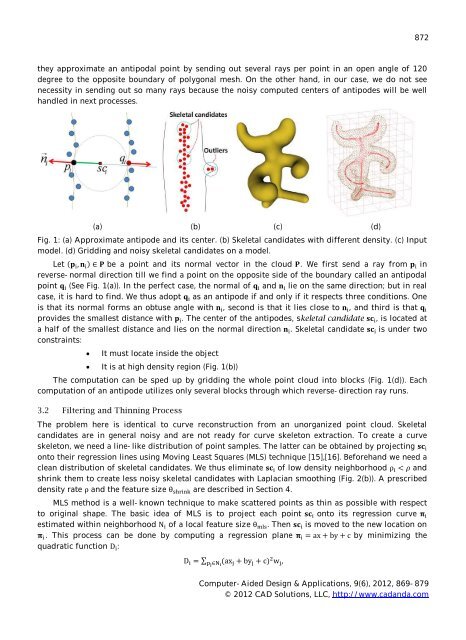
(a) (b) (c) (d)<br />
Fig. 1: (a) Approximate antipode <strong>and</strong> its center. (b) Skeletal c<strong>and</strong>idates with different density. (c) Input<br />
model. (d) Gridding <strong>and</strong> noisy skeletal c<strong>and</strong>idates on a model.<br />
Let ܘ) ୧ ܖǡ ୧ ) ۾ א be a point <strong>and</strong> its normal vector in the cloud .۾ We first send a ray <strong>from</strong> ܘ ୧ in<br />
reverse- normal direction till we find a point on the opposite side of the boundary called an antipodal<br />
point ܙ ୧ (See Fig. 1(a)). In the perfect case, the normal of ܙ ୧ <strong>and</strong> ܖ ୧ lie on the same direction; but in real<br />
case, it is hard to find. We thus adopt ܙ ୧ as an antipode if <strong>and</strong> only if it respects three conditions. One<br />
is that its normal forms an obtuse angle with ܖ ୧ , second is that it lies close to ܖ ୧ , <strong>and</strong> third is that ܙ ୧<br />
provides the smallest distance with ܘ ୧ . The center of the antipodes, skeletal c<strong>and</strong>idate ܋ܛ ୧ , is located at<br />
a half of the smallest distance <strong>and</strong> lies on the normal direction ܖ ୧ . Skeletal c<strong>and</strong>idate ܋ܛ ୧ is under two<br />
constraints:<br />
<br />
<br />
It must locate inside the object<br />
It is at high density region (Fig. 1(b))<br />
The computation can be sped up by gridding the whole point cloud into blocks (Fig. 1(d)). Each<br />
computation of an antipode utilizes only several blocks through which reverse- direction ray runs.<br />
3.2 Filtering <strong>and</strong> Thinning Process<br />
The problem here is identical to curve reconstruction <strong>from</strong> an unorganized point cloud. Skeletal<br />
c<strong>and</strong>idates are in general noisy <strong>and</strong> are not ready for curve skeleton extraction. To create a curve<br />
skeleton, we need a line- like distribution of point samples. The latter can be obtained by projecting ܋ܛ ୧<br />
onto their regression lines using Moving Least Squares (MLS) technique [15],[16]. Beforeh<strong>and</strong> we need a<br />
clean distribution of skeletal c<strong>and</strong>idates. We thus eliminate ܋ܛ ୧ of low density neighborhood ρ ୧ ߩ <strong>and</strong><br />
shrink them to create less noisy skeletal c<strong>and</strong>idates with Laplacian smoothing (Fig. 2(b)). A prescribed<br />
density rate ρ <strong>and</strong> the feature size θ ୱ୦୰୧୬୩ are described in Section 4.<br />
MLS method is a well- known technique to make scattered points as thin as possible with respect<br />
to original shape. The basic idea of MLS is to project each point ܋ܛ ୧ onto its regression curve ૈ ୧<br />
estimated within neighborhood N ୧ of a local feature size θ ୫ ୪ୱ . Then ܋ܛ ୧ is moved to the new location on<br />
ૈ ୧ . This process can be done by computing a regression plane ૈ ୧ = ax + by + c by minimizing the<br />
quadratic function D ୧ :<br />
D ୧ = ∑ (ax ୨ + by ୨ + c) ଶ w ୨ ,<br />
୮ ౠ א <br />
Computer- Aided Design & Applications, 9(6), 2012, 869- 879<br />
© 2012 CAD Solutions, LLC, http://www.cad<strong>and</strong>a.com