A Robust and Centered Curve Skeleton Extraction from 3D Point ...
A Robust and Centered Curve Skeleton Extraction from 3D Point ...
A Robust and Centered Curve Skeleton Extraction from 3D Point ...

Create successful ePaper yourself
Turn your PDF publications into a flip-book with our unique Google optimized e-Paper software.
869<br />
A <strong>Robust</strong> <strong>and</strong> <strong>Centered</strong> <strong>Curve</strong> <strong>Skeleton</strong> <strong>Extraction</strong> <strong>from</strong> <strong>3D</strong> <strong>Point</strong> Cloud<br />
Vanna Sam 1 , Hiroaki Kawata 2 <strong>and</strong> Takashi Kanai 3<br />
1<br />
The University of Tokyo, sam_vanna@graco.c.u- tokyo.ac.jp<br />
2<br />
The University of Tokyo, hiroaki@graco.c.u- tokyo.ac.jp<br />
3<br />
The University of Tokyo, kanai@graco.c.u- tokyo.ac.jp<br />
ABSTRACT<br />
A curve skeleton of a <strong>3D</strong> object is one of the most important structures of the object,<br />
which is extremely useful for many computer graphics applications involving in shape<br />
analysis. Much research has focused on volumetric <strong>and</strong> polygonal mesh models.<br />
However, only a few have been paid attention to point cloud <strong>and</strong> suffered <strong>from</strong> several<br />
limitations such as connectivity or inside- shape information requirements, difficulty<br />
to compute junction nodes, or inappropriate parameter tuning. To resolve these<br />
problems, we propose an effective algorithm for extracting a robust <strong>and</strong> centered<br />
curve skeleton <strong>from</strong> point cloud. The process starts <strong>from</strong> estimating centers of<br />
antipodes of a point cloud, so called skeletal c<strong>and</strong>idates, which are fundamentally<br />
inside the shape; but scattered. We thus filter <strong>and</strong> shrink them to create less- noisy<br />
skeletal c<strong>and</strong>idates before applying one- dimensional Moving Least Squares (MLS) to<br />
build a thin point cloud. The latter is then downsampled to sparse skeletal nodes. With<br />
recent nodes, it is possible to create a smooth curve skeleton; but distorted due to<br />
shrinking <strong>and</strong> thinning (MLS) processes. We thus utilize cross- section plane technique<br />
<strong>and</strong> least squares ellipse fitting to relocate skeletal nodes to create a centered curve<br />
skeleton. The algorithm is validated on many complex models ranging <strong>from</strong> cylindrical<br />
to planar ones, <strong>and</strong> <strong>from</strong> clean to noisy <strong>and</strong> incomplete data. We show that the<br />
extracted curve skeleton is robust to noises <strong>and</strong> under centeredness property.<br />
Keywords: curve skeleton, point cloud, antipode, regression line, ellipse fitting<br />
DOI: 10.3722/cadaps.2012.869- 879<br />
1 INTRODUCTION<br />
A curve skeleton of <strong>3D</strong> complex shape is a compact <strong>and</strong> simple structure basically called 1D curve<br />
which provides sufficient information on geometry <strong>and</strong> topology of the shape. There is no absolute<br />
definition of a curve skeleton <strong>and</strong> several have been proposed in the literature review [7]. It is defined<br />
as the locus of the centers of maximal inscribed balls [4], the centerline of <strong>3D</strong> objects [12], or as the<br />
Computer- Aided Design & Applications, 9(6), 2012, 869- 879<br />
© 2012 CAD Solutions, LLC, http://www.cad<strong>and</strong>a.com
870<br />
rotational symmetry axis of an object [24]. The most commonly- targeted curve skeleton is a onedimensional<br />
poly- segment connecting central points of equidistance to the nearest boundary of the<br />
shape. Due to its simple structure, a curve skeleton is easy to manipulate <strong>and</strong> very useful in many<br />
computer graphics applications which involve in shape analysis such as shape recognition, object<br />
matching <strong>and</strong> retrieval [6], animation transfer, <strong>and</strong> so forth. These applications correspondingly<br />
require several necessary properties among topology preservation, centeredness, robustness to noises,<br />
connectedness (as a single graph), reliability (which guarantees that at least one boundary point is<br />
visible to the curve skeleton), hierarchy <strong>and</strong> reconstructability [7].<br />
The major problem in extracting a curve skeleton is how to compute the shape correctly <strong>and</strong><br />
robustly. Even though numerous algorithms have been developed in the past <strong>and</strong> produced<br />
remarkable results, to our knowledge, much research has been done on only polygonal meshes <strong>and</strong><br />
volumetric models [2],[17],[23], which require full knowledge of models. Some have been also paid<br />
attention to both mesh <strong>and</strong> point cloud models [12],[20],[21]. However, only a few have been focusing<br />
on noisy <strong>and</strong> incomplete data models [5],[24]. The challenge to directly extract a curve skeleton <strong>from</strong><br />
noisy or incomplete data is still on- going because previous research suffers <strong>from</strong> several limitations<br />
such as÷ models must be meshed or watertight [2], curve skeletons at junctions are unreliable <strong>and</strong><br />
hard to compute [20],[24] <strong>and</strong> a lot of efforts are needed in parameter tuning [5],[24].<br />
To overcome these problems, we propose a robust extraction of curve skeleton <strong>from</strong> clean, noisy<br />
<strong>and</strong> incomplete data. There are two key ideas in our method. One is to make our extraction algorithm<br />
robust: We validate the skeletal c<strong>and</strong>idates according to their densities based on filtering <strong>and</strong><br />
shrinking processes. Low density regions of skeletal c<strong>and</strong>idates contribute less in creating a curve<br />
skeleton. They are, thus, considered as noises or outliers <strong>and</strong> are eliminated by filtering process. The<br />
remaining skeletal c<strong>and</strong>idates are reinforced through shrinking process to create ones less noises <strong>and</strong><br />
free <strong>from</strong> outliers. The other is that we utilize ellipse fitting to relocate the skeletal nodes to ensure<br />
that they lie on the center of the model i.e. our curve skeleton is under robustness <strong>and</strong> centeredness<br />
properties.<br />
Our main contributions include (i) a curve skeleton extraction directly <strong>from</strong> point cloud (ii) a<br />
robust extraction <strong>from</strong> noisy <strong>and</strong> incomplete data <strong>and</strong> (iii) a centeredness- guaranteed curve skeleton<br />
defined by ellipse fitting.<br />
The paper is organized as follows. Section 2 presents literature review of curve skeleton extraction<br />
methods <strong>and</strong> related work. In Section 3, we describe details of our proposed algorithm, <strong>and</strong> we show<br />
results <strong>and</strong> discussion of our algorithm on various types of <strong>3D</strong> shapes in Section 4. At the end of the<br />
section, we show a comparison of our algorithm with [5] <strong>and</strong> [24]. Section 5 raises conclusions <strong>and</strong><br />
future work for our method.<br />
2 RELATED WORK<br />
There is a vast literature of curve skeleton starting with the most well- known medial axis [4]. There are<br />
numerous algorithms in extracting curve skeletons in the past. Those algorithms are roughly<br />
categorized into two main groups. For a complete review, we refer readers to [7] <strong>and</strong> [22].<br />
Volumetric methods: In this category, a given <strong>3D</strong> input model is voxelized in <strong>3D</strong> space <strong>and</strong> the<br />
curve skeleton is computed by volumetric thinning or by field- function techniques. In volumetric<br />
thinning [23],[17],[3], boundary voxels so called simple points are iteratively removed until one voxel<br />
thick is found. The curve skeleton in this method is a result of connecting centers of central voxels.<br />
Whereas in field- function techniques [6],[12], distance or force field is defined for each interior point<br />
<strong>and</strong> the ridges of this field correspond to central voxels of the object. The curve skeleton results <strong>from</strong><br />
Computer- Aided Design & Applications, 9(6), 2012, 869- 879<br />
© 2012 CAD Solutions, LLC, http://www.cad<strong>and</strong>a.com
871<br />
connecting those ridges. In summary, this type of methods requires clear information on the inside of<br />
the shape <strong>and</strong> suffers numerical instability caused by inappropriate voxelization resolutions clearly<br />
mentioned in [5],[24]. It is, thus, not suitable for point cloud models.<br />
Geometric Methods: This kind of methods is applicable to both polygonal meshes <strong>and</strong> point<br />
clouds. The most popular techniques involve in using Voronoi diagram [8],[18],[19] to approximate<br />
medial surfaces <strong>and</strong> then prune them to create a curve skeleton. Recent research [2] utilizes Laplacian<br />
smoothing to shrink polygonal mesh to zero volume mesh <strong>and</strong> then fix the connectivity to create a<br />
curve skeleton. This method provides excellent results. However, it is applicable to only polygonal<br />
mesh <strong>and</strong> water- tight models. [5] can be considered as an extension of the previous method for<br />
incomplete point clouds. Each point requires a local creation of one- ring connectivity of neighborhood<br />
for Laplacian operation <strong>and</strong> much attention has to be paid to contraction parameters. The research<br />
produces good results for some models. However, incorrect topology may occur near close- by<br />
structures <strong>and</strong> wrong parameter tuning may lead to a curve skeleton outside the model. Recently, [24]<br />
utilizes cutting plane idea to compute a curve skeleton <strong>from</strong> incomplete point cloud <strong>and</strong> fills in the<br />
missing data to assist surface reconstruction. Cutting planes are well oriented at cylindrical shapes;<br />
but not at non- cylindrical ones, which are normally junction regions. The latter requires special<br />
h<strong>and</strong>ling. However, it seems hard to define <strong>and</strong> guarantee that curve skeletons around junctions are<br />
well connected or centered.<br />
Similar to [20], we attempt to approximate antipodal points <strong>from</strong> the shape <strong>and</strong> their<br />
corresponding centers called skeletal c<strong>and</strong>idates for a curve skeleton. Different <strong>from</strong> [20], we send<br />
only one ray to find the antipode of each point <strong>and</strong> we do not eliminate skeletal c<strong>and</strong>idates at junction<br />
regions. The latter will be well treated in Section 3 <strong>and</strong> the centeredness is verified at the end of the<br />
section.<br />
3 CURVE SKELETON EXTRACTION<br />
<strong>Point</strong>- based models are usually acquired by range scanner or image- based reconstruction techniques.<br />
They are ready to use, easy to h<strong>and</strong>le, <strong>and</strong> do not require any connectivity information or complex<br />
data structures such as polygonal mesh models. Our proposed algorithm focuses on oriented point<br />
clouds to make use of the above advantages. Given a point cloud as an input, the normal direction <strong>and</strong><br />
orientation of a point can be estimated through its neighborhood information [13],[14].<br />
Our algorithm proceeds as follows. We first attempt to compute the center of antipodes of each<br />
point in the cloud by extending its normal in reverse direction till the opposite side of the boundary.<br />
All computed centers are called skeletal c<strong>and</strong>idates. The latter are basically scattered <strong>and</strong> theoretically<br />
lain on medial surface. To conquer the weakness of medial axis, which is sensitive to noisy boundary<br />
surface, we assume skeletal c<strong>and</strong>idates of high density neighborhood contribute better to the<br />
computation of a curve skeleton in the next process. We thus consider skeletal c<strong>and</strong>idates of low<br />
density as outliers or noises. It means that we remove them <strong>and</strong> shrink the remainder by Laplacian<br />
smoothing [25] to form a strong- bond distribution. We then process thinning algorithm using 1D<br />
Moving Least Squares [15],[16] till a line- like thin cloud of skeletal c<strong>and</strong>idates is obtained. The next<br />
process is to extract skeletal nodes necessary for a curve skeleton. The final process is to relocate<br />
those skeletal nodes to the center of the shape. Below are details of each process.<br />
3.1 Antipodes <strong>and</strong> Skeletal C<strong>and</strong>idates<br />
Two points are antipodes if they are diametrically opposite. On a smooth surface, an antipodal point<br />
can defined by extending its normal in reverse direction till the opposite boundary surface [20].<br />
However, in polygonal meshes or point clouds, exact antipodal points are difficult to compute. In [20],<br />
Computer- Aided Design & Applications, 9(6), 2012, 869- 879<br />
© 2012 CAD Solutions, LLC, http://www.cad<strong>and</strong>a.com
872<br />
they approximate an antipodal point by sending out several rays per point in an open angle of 120<br />
degree to the opposite boundary of polygonal mesh. On the other h<strong>and</strong>, in our case, we do not see<br />
necessity in sending out so many rays because the noisy computed centers of antipodes will be well<br />
h<strong>and</strong>led in next processes.<br />
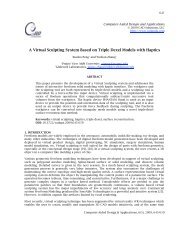
(a) (b) (c) (d)<br />
Fig. 1: (a) Approximate antipode <strong>and</strong> its center. (b) Skeletal c<strong>and</strong>idates with different density. (c) Input<br />
model. (d) Gridding <strong>and</strong> noisy skeletal c<strong>and</strong>idates on a model.<br />
Let ܘ) ୧ ܖǡ ୧ ) ۾ א be a point <strong>and</strong> its normal vector in the cloud .۾ We first send a ray <strong>from</strong> ܘ ୧ in<br />
reverse- normal direction till we find a point on the opposite side of the boundary called an antipodal<br />
point ܙ ୧ (See Fig. 1(a)). In the perfect case, the normal of ܙ ୧ <strong>and</strong> ܖ ୧ lie on the same direction; but in real<br />
case, it is hard to find. We thus adopt ܙ ୧ as an antipode if <strong>and</strong> only if it respects three conditions. One<br />
is that its normal forms an obtuse angle with ܖ ୧ , second is that it lies close to ܖ ୧ , <strong>and</strong> third is that ܙ ୧<br />
provides the smallest distance with ܘ ୧ . The center of the antipodes, skeletal c<strong>and</strong>idate ܋ܛ ୧ , is located at<br />
a half of the smallest distance <strong>and</strong> lies on the normal direction ܖ ୧ . Skeletal c<strong>and</strong>idate ܋ܛ ୧ is under two<br />
constraints:<br />
<br />
<br />
It must locate inside the object<br />
It is at high density region (Fig. 1(b))<br />
The computation can be sped up by gridding the whole point cloud into blocks (Fig. 1(d)). Each<br />
computation of an antipode utilizes only several blocks through which reverse- direction ray runs.<br />
3.2 Filtering <strong>and</strong> Thinning Process<br />
The problem here is identical to curve reconstruction <strong>from</strong> an unorganized point cloud. Skeletal<br />
c<strong>and</strong>idates are in general noisy <strong>and</strong> are not ready for curve skeleton extraction. To create a curve<br />
skeleton, we need a line- like distribution of point samples. The latter can be obtained by projecting ܋ܛ ୧<br />
onto their regression lines using Moving Least Squares (MLS) technique [15],[16]. Beforeh<strong>and</strong> we need a<br />
clean distribution of skeletal c<strong>and</strong>idates. We thus eliminate ܋ܛ ୧ of low density neighborhood ρ ୧ ߩ <strong>and</strong><br />
shrink them to create less noisy skeletal c<strong>and</strong>idates with Laplacian smoothing (Fig. 2(b)). A prescribed<br />
density rate ρ <strong>and</strong> the feature size θ ୱ୦୰୧୬୩ are described in Section 4.<br />
MLS method is a well- known technique to make scattered points as thin as possible with respect<br />
to original shape. The basic idea of MLS is to project each point ܋ܛ ୧ onto its regression curve ૈ ୧<br />
estimated within neighborhood N ୧ of a local feature size θ ୫ ୪ୱ . Then ܋ܛ ୧ is moved to the new location on<br />
ૈ ୧ . This process can be done by computing a regression plane ૈ ୧ = ax + by + c by minimizing the<br />
quadratic function D ୧ :<br />
D ୧ = ∑ (ax ୨ + by ୨ + c) ଶ w ୨ ,<br />
୮ ౠ א <br />
Computer- Aided Design & Applications, 9(6), 2012, 869- 879<br />
© 2012 CAD Solutions, LLC, http://www.cad<strong>and</strong>a.com
873<br />
where w ୨ denotes a weight function. We can then solve MLS problem in 2D i.e. line fitting problem to 2D<br />
points. In our case, we intend to compute discrete curve skeleton, we thus do not need to compute <strong>3D</strong><br />
regression curve; but <strong>3D</strong> regression line. We simply compute <strong>3D</strong> regression line by using the Principle<br />
Component Analysis (PCA). The line passes through the centroid of PCA <strong>and</strong> directs along the<br />
eigenvector of the largest eigenvalue of the covariance matrix of PCA. We iteratively project each point<br />
ܑ onto its <strong>3D</strong> regression line until 1D point cloud is obtained (Fig. 2(c)). The process is repeated four ܋ܛ<br />
times through our experiment <strong>and</strong> results are sufficient enough for skeletal nodes' sampling.<br />
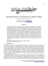
(a) (b) (c) (d)<br />
Fig. 2: <strong>Curve</strong> skeleton extraction process. (a) Skeletal c<strong>and</strong>idates. (b) Filtered <strong>and</strong> skeletal c<strong>and</strong>idates.<br />
(c) MLS projected skeletal c<strong>and</strong>idates. (d) Pre- centered skeletal nodes.<br />
3.3 Skeletal Node Sampling<br />
The previous processes provide projected skeletal c<strong>and</strong>idates sufficiently thin <strong>and</strong> dense enough for<br />
building 1D curve skeleton. We uniformly resample projected skeletal c<strong>and</strong>idates in a large reduction<br />
scale [15] (Fig. 2(d)). We first pick a projected skeletal c<strong>and</strong>idate r<strong>and</strong>omly <strong>from</strong> a thin cloud as a<br />
skeletal node ܖܛ ୩ <strong>and</strong> compute its neighboring points N ୩ within a local feature size θ ୱୟ୫ ୮୪ୣ using KD<br />
tree data structure. We then choose the furthest point in N ୩ <strong>from</strong> ܖܛ ୩ , <strong>and</strong> define it as another skeletal<br />
node ܖܛ ୩ାଵ . The remainder in N ୩ is removed. The process is repeated until no point is left in the stack.<br />
Finally we obtain several dozen of points as shown in Fig. 2(d).<br />
3.4 Centering Process <strong>and</strong> <strong>Curve</strong> <strong>Extraction</strong><br />
Skeletal nodes obtained <strong>from</strong> the previous processes can be used to create a smooth curve skeleton.<br />
However, shrinking <strong>and</strong> thinning processes may distort the centeredness of computed skeletal nodes.<br />
We thus utilize least- squares ellipse fitting in [10],[11] to relocate skeletal nodes. Ellipse fitting process<br />
has to be done in 2D space. We thus need to extract relevant neighborhood N ୩ of each ܖܛ ୩ <strong>and</strong><br />
transform N ୩ <strong>from</strong> <strong>3D</strong> to 2D space before applying ellipse fitting algorithm. We detail the whole<br />
process into three steps as follows <strong>and</strong> the result is shown in Fig. 3(b):<br />
Step 1 (Relevant Neighborhood N ୩ ): We utilize the cutting plane idea introduced in [24] to collect<br />
boundary points within the thickness δ ୮୪ୟ୬ୣ to the plane. The latter passes through the skeletal node<br />
୩ <strong>and</strong> its nearest neighbor. The cutting plane ܖܛ ୩ <strong>and</strong> its orientation is a vector built <strong>from</strong> a node ܖܛ<br />
may pass through multiple branches of the model. To extract relevant neighboring points <strong>from</strong> the<br />
latter, Density- Based Spatial Clustering of Application with Noise (DBSCAN) [9] is a suitable c<strong>and</strong>idate<br />
since we have no information on number of clusters (Fig. 3(a)). The targeted cluster is one whose<br />
centroid is closed to ܖܛ ୩ . Two necessary parameters (eps, MinPts) for DBSCAN are described in Section 4.<br />
Computer- Aided Design & Applications, 9(6), 2012, 869- 879<br />
© 2012 CAD Solutions, LLC, http://www.cad<strong>and</strong>a.com
874<br />
Step 2 (Basis Matrix Estimation): Once relevant neighboring points N ୩ are found, we transform<br />
them <strong>from</strong> <strong>3D</strong> into 2D coordinate system for ellipse fitting process. To estimate an optimized basis<br />
matrix for <strong>3D</strong> projection, we make use of cutting plane optimization problem introduced in [24] such<br />
that the cutting plane orientation is optimized when it is perpendicular to the tangent plane formed<br />
<strong>from</strong> points in N ୩ . The problem can be solved in closed- form by computing three eigenvectors of<br />
covariance matrix ۻ ଷ୶ଷ of normal vectors of points in N ୩ (more detailed in [24]),<br />
X ଶ − X ଶ 2XY − 2XഥYഥ 2XZ − 2XഥZത<br />
ଷ୶ଷ = ൮2XY − 2XഥYഥ ۻ<br />
Y ଶ − Y ଶ ൲, 2YZ − 2YഥZത 2XZ − 2XഥZത 2YZ − 2YഥZത Z ଶ − Z ଶ<br />
where X, Y, Z <strong>and</strong> Xഥ, Yഥ, Zത are r<strong>and</strong>om variables <strong>and</strong> averages of x, y, z components of normals in N ୩<br />
respectively. The three eigenvectors ଵ , ଶ , ଷ of ۻ ଷ୶ଷ can be solved via singular value decomposition.<br />
The projection matrix is then defined as:<br />
ϑ ଵ୶ ϑ ଵ୷ ϑ ଵ<br />
ቍ. ቌϑ ଶ୶ ϑ ଶ୷ ϑ ଶ =ܚ۾<br />
ϑ ଷ୶ ϑ ଷ୷ ϑ ଷ<br />
Step 3 (Least Squares Methods of Ellipse Fitting): In this step, we intend to compute all centers of<br />
ellipses fitted to a set of 2D points in N ୩ for every skeletal node. The center is a correct node if it<br />
locates at the center of the shape <strong>and</strong> lies close to its corresponding skeletal node i.e. the distance<br />
between the center <strong>and</strong> its skeletal node must be smaller than an error ε ୡୣ୬୲ୣ୰ . Otherwise it is neglected.<br />
An ellipse fitting is a particular case of general conic fitting. Below is a short explanation of an<br />
algebraic ellipse fitting (more details in [11]).<br />
F(x, y) = ax ଶ + bxy + cy ଶ + dx + ey + f = 0. (1)<br />
An ellipse is defined by six coefficients (a, b, c, d, e, f) with a constraint b ଶ − 4ac < 0 . (x, y) are<br />
coordinates of 2D points to be fitted to an ellipse. In matrix form (1) can be written as:<br />
F ܝ ∙ ܆ = (܆) ܝ where ܆ = [x ଶ , xy, y ଶ , x, y, 1] ܝ<strong>and</strong> = [a, b, c, d, e, f] . (2)<br />
To find the six coefficients of an ellipse ,ܝ we solve the above equation by minimizing the sum of<br />
squared algebraic distances <strong>from</strong> points to the ellipse:<br />
∑ ܝ min<br />
୨ୀଵ F(x ୨ , y ୨ ) ଶ = min ܝ ∑ ୨ୀଵ ܆)F ୨ ∙ (ܝ ଶ = min ܝ ‖ܝ۲‖ ଶ . (3)<br />
In order to simplify the computation <strong>and</strong> to obtain a proper solution, the constraint b ଶ − 4ac < 0 is<br />
determined to 4ac − b ଶ = 1. The latter can be rewritten in matrix form ܝ = ܝ۱ 1 <strong>and</strong> the solution of the<br />
minimization problem (3) is the eigenvector corresponding to the smallest positive eigenvalue of<br />
generalized eigenproblem.<br />
ଶ ଶ<br />
x ଵ x ଵ y ଵ y ଵ x y 1<br />
0 0 2 0 0 0<br />
۲ ⎛<br />
⋮ ⋮ ⋮ ⋮ ⋮ ⋮<br />
0 −1 0 0 0 0<br />
ଶ ଶ<br />
⎞ ⎛<br />
⎞<br />
with۲ = ⎜x ୨ x ୨ y ୨ y ୨ x ୨ y ୨ 1 ,ܝλ۱ = ܝ۲<br />
2 0 0 0 0 0<br />
⎟ , ۱ = ⎜<br />
0 0 0 0 0 0<br />
⎟.<br />
⋮ ⋮ ⋮ ⋮ ⋮ ⋮<br />
ଶ ଶ 0 0 0 0 0 0<br />
⎝x x y y x y 1⎠ ⎝0 0 0 0 0 0⎠<br />
<strong>Curve</strong> <strong>Extraction</strong>: To construct a curve skeleton, we apply nearest neighbor crust algorithm [1] on<br />
recently centered skeletal nodes (Fig. 3(c)).<br />
Computer- Aided Design & Applications, 9(6), 2012, 869- 879<br />
© 2012 CAD Solutions, LLC, http://www.cad<strong>and</strong>a.com
875<br />
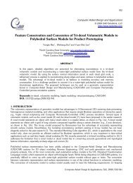
(a) (b) (c)<br />
Fig. 3: Centering Process. (a) Cutting plane with an orientation (red vector) <strong>and</strong> relevant neighborhood.<br />
(b) Difference between pre- centered (Red) <strong>and</strong> centered skeletal nodes (Green). (c) <strong>Curve</strong> skeleton.<br />
4 RESULTS AND DISCUSSION<br />
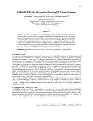
We have demonstrated our algorithm on different models including clean, noisy <strong>and</strong> incomplete<br />
data. Our algorithm works well even in low resolution model (2K points) <strong>and</strong> provides not much<br />
different results with high resolution ones (Fig.4). Since there is no need to use a great number of<br />
points for a curve skeleton extraction in our algorithm, we thus downsample the tested models to<br />
approximately 10K points for efficiency.<br />
(a) (b) (c)<br />
Fig. 4: Consistency of our curve skeleton. (a) 2K points. (b) 8K points. (c) 15K points.<br />
Parameters: The parameters (ρ, θ ୱ୦୰୧୬୩ , θ ୫ ୪ୱ , θ ୱୟ୫ ୮୪ୣ , δ ୮୪ୟ୬ୣ , ϵ ୡୣ୬୲ୣ୰ , eps, MinPts) can be independently<br />
controlled to extract a curve skeleton adapting to particular topology of the model. Tuning many<br />
parameters is a tedious task <strong>and</strong> it takes much effort to find good ones. In our case, we empirically<br />
notice that there is no need to tune all eight parameters; but two of them – ρ <strong>and</strong> θ ୱ୦୰୧୬୩ . In this paper,<br />
we choose ρ <strong>from</strong> 6 to 18 points (a point whose neighboring points are less than ρ is considered as<br />
outlier) <strong>and</strong> θ ୱ୦୰୧୬୩ is set <strong>from</strong> 1.5 to 2.5% of the diagonal of the bounding box. Other parameters are<br />
estimated as θ ୫ ୪ୱ = 2θ ୱ୦୰୧୬୩ , θ ୱୟ୫ ୮୪ୣ = δ ୮୪ୟ୬ୣ = ϵ ୡୣ୬୲ୣ୰ = eps = θ ୱ୦୰୧୬୩ , MinPts = 4 as default of DBSCAN.<br />
Discussion: Fig. 5 shows the effectiveness of our method on several different shapes. It works<br />
very well on especially cylindrical or elliptical shapes (Fig. 4) & (Fig. 5(a, c, g, h)). For the planar model<br />
in Fig. 5(b), our method generates very scattered skeletal c<strong>and</strong>idates at the beginning as same as<br />
Medial Axis Transform does. However, through filtering <strong>and</strong> smoothing processes, low density regions<br />
Computer- Aided Design & Applications, 9(6), 2012, 869- 879<br />
© 2012 CAD Solutions, LLC, http://www.cad<strong>and</strong>a.com
876<br />
are eliminated <strong>and</strong> most of pre- centered skeletal nodes are already at the center of the shape.<br />
Projecting <strong>and</strong> centering processes ensure that skeletal nodes locate at the center of the shape. Our<br />
result for this model is quite different <strong>from</strong> medial axis; but it shows another flavor for a curve<br />
skeleton on planar shapes.<br />
(a) (b) (c) (d)<br />
(e) (f) (g) (h)<br />
Fig. 5: Results of our method on various shapes including cylindrical <strong>and</strong> flat regions.<br />
Our method is robust to noises (Fig. 6) because even though noisy points create noisy skeletal<br />
c<strong>and</strong>idates or generate outliers, it will be well cleaned up through filtering <strong>and</strong> shrinking processes.<br />
Fig. 6(b), (d), (e) shows robustness of our method against noisy <strong>and</strong> incomplete data. We do not<br />
evaluate how much our method can resist to noises. The incomplete models Fig. 6(b) <strong>and</strong> Fig. 6(d) are<br />
created manually by removing some parts. The model Fig. 6(d) is missing almost half of the data. As<br />
for the noisy model Fig. 6(e), it is created by scattering approximately 30% of the whole points <strong>from</strong> its<br />
original boundary points. Even in such extreme condition (large missing data <strong>and</strong> high level of noises<br />
<strong>and</strong> outliers), our method extracts well the curve skeleton.<br />
Time Complexity: The most time- consuming process in our algorithm is the computation of<br />
skeletal c<strong>and</strong>idates. To speed up the computation, we utilize gridding technique (5 grids along the<br />
longest bounding box) to divide point cloud into smaller blocks <strong>and</strong> each computation uses several<br />
blocks through which the normal direction runs. Although the whole algorithm is implemented in<br />
C+ + , the gridding algorithm is not yet optimized. For 10K points, it takes approximately 6 seconds for<br />
skeletal c<strong>and</strong>idates, 1.8 seconds for filtering <strong>and</strong> shrinking process, 2 seconds for thinning process,<br />
0.9 seconds for centering process (ellipse fitting). Thus, the whole process takes approximately 7<br />
seconds for 10K points, which are measured on a st<strong>and</strong>ard PC with Core i7- 860 CPU.<br />
Comparison: Fig. 6 shows the comparison of our algorithm with Laplacian- based contraction on<br />
point cloud [5] <strong>and</strong> Rotational Symmetry Axis (ROSA) [24]. Both methods extract good curve skeletons<br />
Computer- Aided Design & Applications, 9(6), 2012, 869- 879<br />
© 2012 CAD Solutions, LLC, http://www.cad<strong>and</strong>a.com
877<br />
<strong>from</strong> point cloud model (Fig.6(c)). To the best of our parameter tuning for [5] <strong>and</strong> [24], the overall<br />
results show that our algorithm works better in term of centeredness <strong>and</strong> robustness to incomplete<br />
data <strong>and</strong> one with noises <strong>and</strong> outliers. It shows that [5] <strong>and</strong> [24] provide good curve skeletons on<br />
incomplete data (Fig. 6(b, d)) to some extent. [5] <strong>and</strong> [24] cannot generate a curve skeleton when some<br />
blocks of data are missing (Fig.6(b)) <strong>and</strong> fail to create a good curve skeletons with presence of very<br />
large missing data Fig.6(d). They both fails on noisy data with some outliers (Fig. 6(e)).<br />
[5] extracts good curve skeleton <strong>from</strong> planar shape (Fig.6(a)), whereas [24] cannot define a curve<br />
skeleton on planar shapes as mentioned in the paper. On the other h<strong>and</strong>, even though our method<br />
generates, for planar shapes, a curve skeleton different <strong>from</strong> [5] <strong>and</strong> medial axis, it stays well under<br />
centerline definition.<br />
Laplacian- based contraction [5]<br />
ROSA [24]<br />
Our method<br />
(a) (b) (c) (d) (e)<br />
Fig. 6: Comparison of our method with Laplacian- based contraction [5] <strong>and</strong> Rotational Symmetry Axis<br />
(ROSA) [24].<br />
Limitations: Our method provides very high accuracy on branch regions or cylindrical shapes Fig.<br />
5(a, g). However, the accuracy tends to decline at join regions due to lack of skeletal nodes, for<br />
example at the front part of Dino model (Fig. 5(f)). This is due to the instability of cutting plane<br />
optimization, which results in incorrect neighborhoods for ellipse fitting. Consequently, skeletal nodes<br />
are largely eliminated at those joint regions.<br />
Computer- Aided Design & Applications, 9(6), 2012, 869- 879<br />
© 2012 CAD Solutions, LLC, http://www.cad<strong>and</strong>a.com
878<br />
Another limitation is that details on coarse parts of the model are sometimes reduced (Fig.5(e))<br />
because our algorithm includes filtering, shrinking, <strong>and</strong> thinning processes. All of these processes<br />
tend to pull scattered skeletal c<strong>and</strong>idates together to form highly concentrated nodes in which<br />
scattered points at the end part of the model are either eliminated or shrunk to some extent. Lowering<br />
local feature sizes θ ୱ୦୰୧୬୩ , θ ୫ ୪ୱ <strong>and</strong> density rate ρ may solve the problem.<br />
Similar to the above limitation, skeletal c<strong>and</strong>idates may be removed due to low density rates, for<br />
example, at thin planar shape of the model (Fig. 5(d)). Through filtering <strong>and</strong> shrinking processes,<br />
skeletal c<strong>and</strong>idates at the central seating part of the model are mostly removed. However, cylindrical<br />
parts are well preserved <strong>and</strong> the frame of the seating part still exists because they are high density<br />
regions. The frame is, then, cleaned up through centering process because, far <strong>from</strong> theirs<br />
corresponding skeletal nodes, the centers of fitted ellipses appear at the center of seating part of the<br />
model. Consequently, centered skeletal nodes of the frame part are neglected.<br />
5 CONCLUSIONS AND FUTURE WORK<br />
We have proposed a direct extraction of curve skeleton <strong>from</strong> point cloud. Various models ranging <strong>from</strong><br />
cylindrical to flat shapes of both clean <strong>and</strong> incomplete situation have been evaluated. The extracted<br />
curve skeletons are remarkable – robust to high noisy boundary points due to filtering <strong>and</strong> shrinking<br />
processes, <strong>and</strong> under centeredness- guaranteed property demonstrated by ellipse fitting. To achieve<br />
good results, parameter tuning is required; but it is an easy task done by modifying a local feature size<br />
<strong>and</strong> choosing the density rate within the size.<br />
For future work, we would like to generate parameters automatically for our algorithm <strong>and</strong><br />
implement it on raw scanning data with large missing parts or less scans per model. To exploit the<br />
computed curve skeleton for some applications such as surface reconstruction or shape matching is<br />
also our potential task.<br />
ACKNOWLEDGEMENTS<br />
The availability of source code [5] <strong>and</strong> [24] is of much help in the comparison section. Models used in<br />
this paper are obtained <strong>from</strong> the AIM@SHAPE repository.<br />
REFERENCES<br />
[1] Amanta, N.; Bern, M.; Eppstein, D.: Crust <strong>and</strong> the Beta- <strong>Skeleton</strong>: Combinatorial <strong>Curve</strong>, Graphical<br />
Models <strong>and</strong> Image Processing, 60(2), 1998, 125- 135. DOI:10.1006/gmip.1998.0465<br />
[2] Au, K.- C. O.; Thai, C.- L.; Chu, H.- K.; Cohen- Or, D.; Lee, T.- Y.: <strong>Skeleton</strong> <strong>Extraction</strong> by Mesh<br />
Contraction, ACM Transactions on Graphics, 27 (3), 2007, 44:1- 44:10. DOI:0.1145/1399504.<br />
1360643<br />
[3] Bertr<strong>and</strong>, G.; Aktouf, Z.: Three- Dimensional Thinning Algorithm Using Subfields. Vision<br />
Geometry III, Proc. 2356, 1994, 113- 124. DOI:10.1109/TPAMI.2002.1114851<br />
[4] Blum, H.: A Transformation for Extracting New Descriptors of Shape, In Models for the<br />
Perception of Speech <strong>and</strong> Visual Form, MIT Press, 1967, 362- 380.<br />
[5] Cao, J.; Tagliasacchi, A.; Olson, M.; Zhang, H.; Su, Z.: <strong>Point</strong> Cloud <strong>Skeleton</strong>s via Laplacian- Based<br />
Contraction, Shape Modeling International Conference (SMI), 2010, 187- 197. DOI:<br />
10.1109/SMI.2010.25<br />
[6] Cornea, N. D.; Demirci, M. F.; Silver, D.; Shokouf<strong>and</strong>eh, A.; Dickinson, S. J.; Kantor, P. B.: <strong>3D</strong> Object<br />
Retrieval Using Many- to- many Matching of <strong>Curve</strong> <strong>Skeleton</strong>s, Shape Modeling <strong>and</strong> Applications<br />
2005 International Conference, 2005, 366- 371. DOI:10.1109/SMI.2005.1<br />
Computer- Aided Design & Applications, 9(6), 2012, 869- 879<br />
© 2012 CAD Solutions, LLC, http://www.cad<strong>and</strong>a.com
879<br />
[7] Cornea, N. D.; Silver, D.; Min, P.: <strong>Curve</strong>- <strong>Skeleton</strong> Properties, Applications <strong>and</strong> Algorithms, IEEE<br />
Transactions on Visualization <strong>and</strong> Computer Graphics, 13 (3), 2007, 530- 548.<br />
DOI:10.1109/TVCG.2007.1002<br />
[8] Dey, T. K.; Sun, J.: Defining <strong>and</strong> Computing <strong>Curve</strong> <strong>Skeleton</strong>s with Medial Geodesic Functions, SGP<br />
'06 Proceedings of the Fourth Eurographics Symposium on Geometry Processing, 2006.<br />
[9] Everitt, B.; L<strong>and</strong>au, S.; Leese, M.; Stahl, D.: Cluster Analysis, In Miscellaneous Clustering Methods,<br />
A John Wiley <strong>and</strong> Sons, 5 ed., 2011.<br />
[10] Fitzgibbon, A.; Pilu, M.; Fisher, R. B.: Direct Least Square Fitting of Ellipses, IEEE Transactions on<br />
Pattern Analysis <strong>and</strong> Machine Intelligence, 21 (5), 1999, 475- 480. DOI:10.1109/34.765658<br />
[11] Halif, R.; Flusser, J.: Numerically Stable Direct Least Squares Fitting of Ellipses, The Sixth<br />
International Conference in Central Europe on Computer Graphics <strong>and</strong> Visualization, 21 (5),<br />
1998, 125- 132.<br />
[12] Hassouna, M. S.; Farag, A. A.: <strong>Robust</strong> Centerline <strong>Extraction</strong> Framework Using Level Sets, In IEEE<br />
Conference on Computer Vision <strong>and</strong> Pattern Recoginition (CVPR), 2005, 458- 465.<br />
DOI:10.1109/CVPR.2005.306<br />
[13] Hoppe, H.; DeRose, T.; Duchamp, T.; McDonald, J.; Stuetzle, W.: Surface Reconstruction <strong>from</strong><br />
Unorganized <strong>Point</strong>s, Proc. ACM SIGGRAPH, 1992, 71- 78. DOI:10.1145/142920.134011<br />
[14] Huang, H.; Li, D.; Zhang, H.; Ascher, U.; Cohen- Or, D.: Consolidation of Unorganized <strong>Point</strong> Clouds<br />
for Surafce Reconstruction, ACM Transactions on Graphics, 28 (5), 2009. DOI:10.1145/1618452.<br />
1618522<br />
[15] Lee, I.- K.: <strong>Curve</strong> Reconstruction <strong>from</strong> Unorganized <strong>Point</strong>s, Computer Aided Geometric Design, 17<br />
(2), 2000, 161- 177. DOI:10.1016/S0167- 8396(99)00044- 8<br />
[16] Levin, D.: The Approximation Power of Moving Least- Squares, Mathematics of Computation, 67<br />
(224), 1998, 1517- 1531.<br />
[17] Ma, C.- M.; Wan, S.- Y.; Lee, J.- D.: Three- Dimensional Topology Preserving Reduction on the 4-<br />
Subfields, IEEE Trans. on Pattern Analysis <strong>and</strong> Machine Intelligence, 24 (12), 2002, 1594- 1605.<br />
DOI:10.1109/TPAMI.2002.1114851<br />
[18] Ogniewicz, R.; Ilg, M.: A Multiscale MAT <strong>from</strong> Voronoi Diagrams: the <strong>Skeleton</strong>- Space <strong>and</strong> its<br />
Application to Shape Description <strong>and</strong> Decomposition, Aspects of Visual Form Processing, World<br />
Scientific, 1994.<br />
[19] Ogniewicz, R.; Kubler, O.: Voronoi <strong>Skeleton</strong>s: Theory <strong>and</strong> Applications, IEEE Computer Society<br />
Conference on Computer Vision <strong>and</strong> Pattern Recognition, 1992, 63- 69. DOI:10.1109/CVPR.1992.<br />
223226<br />
[20] Shapira, L.; Shamir, A.; Cohen- Or, D.: Consistent Mesh Partitioning <strong>and</strong> <strong>Skeleton</strong>isation Using the<br />
Shape Diameter Function, Visual Computing, 24 (4), 2008, 249- 259. DOI:10.1007/s00371- 007-<br />
0197- 5<br />
[21] Sharf, A.; Lewiner, T.; Shamir, A.; Kobbelt, L.: On- The- Fly <strong>Curve</strong>- <strong>Skeleton</strong> Compuation for <strong>3D</strong><br />
Shapes, Computer Graphics Forum, 26 (3), 2007, 323- 328.<br />
[22] Siddiqi, K.; Pizer, S. M.: Medial Representations : Mathematics, Algorithms <strong>and</strong> Applications,<br />
Springer, 2009.<br />
[23] Svensson, S.; Nystrom, I.; Sanniti di Baja, G.: <strong>Curve</strong> <strong>Skeleton</strong>ization of Surface- Like Objects in <strong>3D</strong><br />
Images Guided by Voxel Classification, Pattern Recognition Letters, 23, 2002, 1419- 1426.<br />
[24] Tagliasacchi, A.; Zhang, H.; Cohen- Or, D.: <strong>Curve</strong> <strong>Skeleton</strong> <strong>Extraction</strong> <strong>from</strong> Incomplete <strong>Point</strong><br />
Cloud, ACM Transactions on Graphics, 28 (3), 2009, 71:1- 71:9. DOI:10.1145/1531326.1531377<br />
[25] Vollmer, J.; Mencl, R.; Muller, H.: Improved Laplacian Smoothing of Noisy Surface Meshes,<br />
Computer Graphics Forum, 18 (3), 1999, 131- 138.<br />
Computer- Aided Design & Applications, 9(6), 2012, 869- 879<br />
© 2012 CAD Solutions, LLC, http://www.cad<strong>and</strong>a.com