A Robust and Centered Curve Skeleton Extraction from 3D Point ...

874
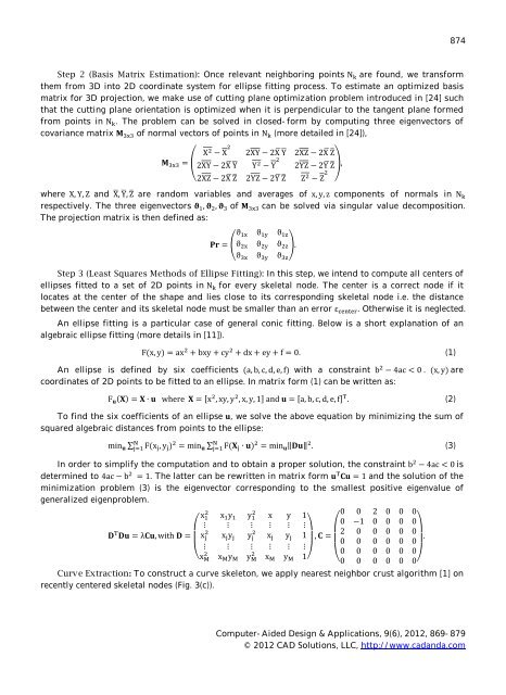
Step 2 (Basis Matrix Estimation): Once relevant neighboring points N ୩ are found, we transform
them from 3D into 2D coordinate system for ellipse fitting process. To estimate an optimized basis
matrix for 3D projection, we make use of cutting plane optimization problem introduced in [24] such
that the cutting plane orientation is optimized when it is perpendicular to the tangent plane formed
from points in N ୩ . The problem can be solved in closed- form by computing three eigenvectors of
covariance matrix ۻ ଷ୶ଷ of normal vectors of points in N ୩ (more detailed in [24]),
X ଶ − X ଶ 2XY − 2XഥYഥ 2XZ − 2XഥZത
ଷ୶ଷ = ൮2XY − 2XഥYഥ ۻ
Y ଶ − Y ଶ ൲, 2YZ − 2YഥZത 2XZ − 2XഥZത 2YZ − 2YഥZത Z ଶ − Z ଶ
where X, Y, Z and Xഥ, Yഥ, Zത are random variables and averages of x, y, z components of normals in N ୩
respectively. The three eigenvectors ଵ , ଶ , ଷ of ۻ ଷ୶ଷ can be solved via singular value decomposition.
The projection matrix is then defined as:
ϑ ଵ୶ ϑ ଵ୷ ϑ ଵ
ቍ. ቌϑ ଶ୶ ϑ ଶ୷ ϑ ଶ ‏=ܚ۾
ϑ ଷ୶ ϑ ଷ୷ ϑ ଷ
Step 3 (Least Squares Methods of Ellipse Fitting): In this step, we intend to compute all centers of
ellipses fitted to a set of 2D points in N ୩ for every skeletal node. The center is a correct node if it
locates at the center of the shape and lies close to its corresponding skeletal node i.e. the distance
between the center and its skeletal node must be smaller than an error ε ୡୣ୬୲ୣ୰ . Otherwise it is neglected.
An ellipse fitting is a particular case of general conic fitting. Below is a short explanation of an
algebraic ellipse fitting (more details in [11]).
F(x, y) = ax ଶ + bxy + cy ଶ + dx + ey + f = 0. (1)
An ellipse is defined by six coefficients (a, b, c, d, e, f) with a constraint b ଶ − 4ac < 0 . (x, y) are
coordinates of 2D points to be fitted to an ellipse. In matrix form (1) can be written as:
F ܝ ∙ ܆ = ‏(܆)‏ ܝ where ܆‏ = [x ଶ , xy, y ଶ , x, y, 1] ܝ‏and = [a, b, c, d, e, f] . (2)
To find the six coefficients of an ellipse ‏,ܝ we solve the above equation by minimizing the sum of
squared algebraic distances from points to the ellipse:
∑ ܝ min
୨ୀଵ F(x ୨ , y ୨ ) ଶ = min ܝ ∑ ୨ୀଵ ܆)‏F ୨ ∙ ‏(ܝ ଶ = min ܝ ‏‖ܝ‎۲‎‏‖‏ ଶ . (3)
In order to simplify the computation and to obtain a proper solution, the constraint b ଶ − 4ac < 0 is
determined to 4ac − b ଶ = 1. The latter can be rewritten in matrix form ܝ = ܝ‎۱‎ 1 and the solution of the
minimization problem (3) is the eigenvector corresponding to the smallest positive eigenvalue of
generalized eigenproblem.
ଶ ଶ
x ଵ x ଵ y ଵ y ଵ x y 1
0 0 2 0 0 0
۲ ⎛
⋮ ⋮ ⋮ ⋮ ⋮ ⋮
0 −1 0 0 0 0
ଶ ଶ
⎞ ⎛
⎞
with۲ = ⎜x ୨ x ୨ y ୨ y ୨ x ୨ y ୨ 1 ‏,ܝλ۱‎ = ܝ‎۲‎
2 0 0 0 0 0
⎟ , ۱ = ⎜
0 0 0 0 0 0
⎟.
⋮ ⋮ ⋮ ⋮ ⋮ ⋮
ଶ ଶ 0 0 0 0 0 0
⎝x x y y x y 1⎠ ⎝0 0 0 0 0 0⎠
Curve Extraction: To construct a curve skeleton, we apply nearest neighbor crust algorithm [1] on
recently centered skeletal nodes (Fig. 3(c)).
Computer- Aided Design & Applications, 9(6), 2012, 869- 879
© 2012 CAD Solutions, LLC, http://www.cadanda.com