470 kb pdf - DR CAJ Appelo -- HYDROCHEMICAL CONSULTANT
470 kb pdf - DR CAJ Appelo -- HYDROCHEMICAL CONSULTANT
470 kb pdf - DR CAJ Appelo -- HYDROCHEMICAL CONSULTANT

You also want an ePaper? Increase the reach of your titles
YUMPU automatically turns print PDFs into web optimized ePapers that Google loves.
MULTICOMPONENT DIFFUSION IN CLAYS<br />
<strong>CAJ</strong> <strong>Appelo</strong> 1<br />
(1) Hydrochemical Consultant. Amsterdam<br />
ABSTRACT<br />
Transport processes in clays are difficult to quantify but are a key-point for deducing the properties of these<br />
materials for waste containment. To improve the situation, version 2.13 of PHREEQC was extended with<br />
multicomponent diffusion and anion exclusion in a diffuse double layer. With it, both laboratory and in-situ<br />
diffusion experiments can be modeled in a comprehensive manner. Application examples are discussed, and<br />
an experiment in Opalinus Clay in Mont Terri (investigated in the framework of possible storage of nuclear<br />
waste in Switzerland) is presented.<br />
Key words: Clays, multicomponent diffusion, PHREEQC, Mont Terri experiment<br />
1. INTRODUCTION<br />
Clays have rather ideal properties for waste containment in the field, but the transport processes are<br />
still difficult to quantify precisely. The dominant transport mode is diffusive and different porewater<br />
diffusion coefficients have been measured for various solutes. However, almost all the models<br />
calculate transport in clays assuming that one and the same diffusion coefficient applies for all the<br />
solutes. Precipitation reactions are usually calculated assuming equilibrium, but this gives wrong<br />
results that would have been noted immediately if the model discretization had been changed. Finally,<br />
the transport properties of clays are dependent on the extent of the double layer that envelops the clay<br />
minerals, but again, this well-accepted feature is not yet accounted for in geochemical transport<br />
models.<br />
Version 2.13 of the hydrogeochemical transport model PHREEQC (Parkhurst and <strong>Appelo</strong>, 1999)<br />
has been extended with a multicomponent diffusion module that may offer some improvement<br />
(<strong>Appelo</strong> and Wersin, 2007). The impetus was provided by detailed diffusion experiments in Opalinus<br />
Clay with various tracers (Wersin et al., 2004). The basic theory for calculating multicomponent<br />
diffusion with a zero charge flux is presented, and various application examples are given.<br />
2. MULTICOMPONENT DIFFUSION<br />
Fick’s laws calculate diffusion from concentration gradients and divergences. However, a more<br />
general equation would employ the electrochemical potential µ, rather than the concentration. The<br />
electrochemical potential is:<br />
µ = µ 0 + RT ln a + zFψ (1)<br />
where µ 0 is the standard potential (J/mol), R is the gas constant (8.314 J/K/mol), T is the absolute<br />
temperature (K), a is the activity (-), z is the charge number (-), F is the Faraday constant (96485<br />
J/V/eq), and ψ is the potential (V). The activity is related to concentration by a = γ c/c 0 , where γ is the<br />
activity coefficient (-) and c 0 is the standard state (1 mol/kg H 2 O, assumed equal to 1 mol/L in the<br />
following).<br />
The diffusive flux of species i in solution as a result of chemical and electrical potential gradients<br />
is:<br />
Water pollution in natural porous media; Candela, L., Vadillo, I., Aagaard, P., Eds.; Instituto<br />
Geológico de España: Madrid, 2007 3
J<br />
i<br />
=<br />
uici<br />
∂µ i<br />
−<br />
| z | F ∂x<br />
i<br />
−<br />
uizic<br />
| z |<br />
i<br />
i<br />
∂ψ<br />
∂x<br />
(2)<br />
where J i is the flux of species i (mol/m 2 /s), and u i is the mobility in water (m 2 /s/V). The mobility is<br />
related to the tracer diffusion coefficient D w, i (m 2 /s) by:<br />
ui<br />
RT<br />
D w,i = (3)<br />
| z | F<br />
The gradient of the electrical potential (∂ψ/∂x) in Equation (2) originates from different transport<br />
velocities of ions, which creates charge and an associated potential. This electrical potential may differ<br />
from the one used in Equation (1), which comes from a charged surface and is fixed, without inducing<br />
electrical current.<br />
If there is no electrical current, Σ zii Jii = 0. This zero-charge flux condition permits to express the<br />
electrical potential gradient as a function of the other terms in Equation (2) and to obtain (Vinograd<br />
and McBain, 1941; Ben-Yaakov, 1972, Cussler, 1984):<br />
i<br />
J<br />
i<br />
= − D<br />
w,i<br />
⎛ ∂ln(<br />
γ ⎞ ∂<br />
⎜<br />
i ) c<br />
+<br />
⎟<br />
i<br />
1<br />
⎝ ∂ln(<br />
c ⎠<br />
∂x<br />
i )<br />
+<br />
D<br />
w,i<br />
z c<br />
i<br />
i<br />
⎛ ∂ln(<br />
γ )<br />
⎞ ∂c<br />
n<br />
∑ ⎜<br />
j<br />
⎟<br />
j<br />
Dw,<br />
j z j + 1<br />
j = 1<br />
∂<br />
⎝<br />
∂ln(<br />
c j ) x<br />
⎠<br />
n<br />
2<br />
∑ Dw,<br />
j z jc<br />
j<br />
j = 1<br />
(4)<br />
where subscript j is introduced to show that these species stem from the potential term.<br />
Equation (4) looks formidable, but inspecting it piecewise will show that the terms involved are<br />
known: they consist of charge numbers and diffusion coefficients (which can be constants at a given<br />
time and place), and concentrations and activity coefficients (which are given by the space<br />
discretization of the model). Thus, the flux of any solute species can be calculated at any time,<br />
iteration (for maintaining electrical neutrality) is not necessary. The equation is valid even if the<br />
solution is not electrically neutral since any charge imbalance that may exist (notably in the diffuse<br />
double layer) is maintained by the zero-charge flux condition. The zero-charge and electroneutrality<br />
conditions have led to discussions in the geochemical literature that ended up pointless (Boudreau et<br />
al., 2004).<br />
2.1. An example: uphill diffusion (after Lichtner, 1995)<br />
We fill a tube with 0.1 mM NaCl and 0.1 mM HNO 3 solution, the pH is 4. We make another<br />
solution with the same NaCl concentration, but with 0.001 mM HNO 3 , the pH is 6. This is the<br />
boundary solution with constant concentrations over time, shown in Figure 1. The figures are copies of<br />
the charts from PHREEQC for Windows, transformed into grayscale, and clearer by coloring when<br />
run on the computer; input-files are available on request to the author, appt@xs4all.nl.<br />
Obviously, H + and NO 3 - are going to diffuse from the column. On the other hand, the concentration<br />
gradients of Na + and Cl - are zero (dc/dx = 0), and their concentrations remain constant according to<br />
Fick’s law. The concentration pattern that results after 1 hour diffusion according to Fick is shown in<br />
Figure 2.<br />
Water pollution in natural porous media; Candela, L., Vadillo, I., Aagaard, P., Eds.; Instituto<br />
Geológico de España: Madrid, 2007 4
Figure 1. Initial conditions in a column example of<br />
multicomponent diffusion. The NaCl concentration is the same<br />
in the boundary solution and in the column; the concentration of<br />
HNO 3 in the column is the same as NaCl (pH = 4, symbols<br />
overlap), but 100 times lower in the boundary solution (pH =<br />
6).<br />
Figure 2. Concentrations in the column after 1 hour<br />
diffusion calculated according to classical diffusion<br />
(Fick) theory. Note that the concentrations of H + and<br />
NO 3 - decrease by diffusion, while Na + and Cl - remain<br />
constant.<br />
However, the diffusion coefficient of H + is about 5 times higher than of NO - 3 , and we can expect<br />
that H + diffuses quicker from the column. The effect can be modeled with PHREEQC’s<br />
multicomponent diffusion module, in which all the solutes diffuse according to their own diffusion<br />
coefficient. The resulting concentration pattern in Figure 3 shows indeed that more H + has diffused out<br />
of the column than in the previous case. Remarkable in Figure 3 is also, that the Na + concentration<br />
bulges upward, although the initial concentration gradient was zero everywhere. On the other hand,<br />
the Cl - concentration has decreased, despite the initially zero concentration gradient which, according<br />
to Fick’s first law, gives a zero flux.<br />
Figure 3. Concentrations in the column after 1 hour diffusion calculated with multicomponent diffusion theory.<br />
These results can be explained as follows. After some time, the column contains more NO 3 - than<br />
H + . Na + that enters the column, and Cl - which leaves the column balance the resulting negative charge.<br />
The diffusion of Na + and Cl - starts although the initial concentration gradient is zero, and continues<br />
even against the concentration gradient that develops. This is a consequence of the zero charge flux<br />
condition that is used to calculate multicomponent diffusion. It is of interest to note that the final stage<br />
in the column, when all the concentrations are equal to the ones in the boundary solution, is reached<br />
quicker with multicomponent diffusion.<br />
Water pollution in natural porous media; Candela, L., Vadillo, I., Aagaard, P., Eds.; Instituto<br />
Geológico de España: Madrid, 2007 5
3. PRECIPITATION REACTIONS IN DIFFUSION CALCULATIONS. EFFECTS OF GRID-SIZE<br />
Numerical models must be checked, if possible, by comparing with an analytical solution. Another,<br />
easier test is to change the gridsize and timestep. But, it has not been well appreciated that the grid size<br />
affects the results of diffusion calculations if equilibrium is assumed with solid phases. To understand<br />
what is going on, let’s model an experiment of Pina et al. (2000), who precipitated scheelite (CaWO 4 )<br />
in a column by letting CaCl 2 and Na 2 WO 4 solutions diffuse from the column ends over 30 days<br />
(Figure 4).<br />
Figure 4. The setup of the diffusion experiment of Pina et al. (2000) in which scheelite precipitates by diffusion of Ca 2+ and<br />
WO 4 2- from the two column-ends.<br />
First, the calculation is done with classical diffusion theory, i.e. all the solutes diffuse at the same<br />
speed and scheelite precipitates to equilibrium where supersaturation is reached, which happens<br />
almost exclusively in the center-cell (Figure 5). With 10 mm cells, 0.09 L scheelite precipitates per L<br />
pore water; with 3.33 mm cells, the amount increases to 0.27 L, and so on. The relative amount of<br />
scheelite in the center-cell increases continuously when the grid is further refined. If the cell-size is<br />
decreased to 1 mm, the amount of scheelite will exceed the pore volume, which is of course<br />
impossible.<br />
Figure 5. Precipitation of scheelite to equilibrium in a diffusion experiment calculated with 10 mm and 3.33 mm grid cells<br />
and the same diffusion coefficient for all solutes. Precipitation takes place in the center cell, irrespective of the grid size, and<br />
relative amounts increase indefinitely as the grid is refined.<br />
The situation improves if the calculation is done with a kinetic precipitation rate that is sufficiently<br />
slow to let the solutes pass the center cell and precipitate further away. The results then become<br />
independent of grid refinement, as illustrated in Figure 6.<br />
Water pollution in natural porous media; Candela, L., Vadillo, I., Aagaard, P., Eds.; Instituto<br />
Geológico de España: Madrid, 2007 6
Figure 6. Precipitation of scheelite becomes independent of grid size if a kinetic rate is used that allows solutes to pass the<br />
center cell.<br />
Kinetics is required in the model anyhow, since scheelite did not precipitate to equilibrium in the<br />
experiment. Pina et al. (2000) observed that precipitation occurred only when the solute ratios of Ca 2+<br />
2-<br />
and WO 4 were within certain limits. Apparently, a high supersaturation, as result of a high<br />
concentration of only one component, is insufficient to engender precipitation if the concentration of<br />
another component that is needed in the precipitate is too small. Pina et al. also found that the zone<br />
with scheelite was displaced away from the center towards the column end where the Na 2 WO 4<br />
solution entered. Similar features were noted already for other minerals by Prieto et al. (1990, 1997).<br />
A kinetic rate was defined in the PHREEQC input file that started the homogeneous precipitation<br />
of scheelite when the saturation ratio attained 10 4 (Pina et al.), and when the activity ratio [Ca 2+ ] /<br />
[WO 4 2- ] ranged from 0.1 to 10. The latter requirement gives a block-like precipitation zone without the<br />
tailing that is visible in Figure 6. The off-center displacement of the precipitation zone was modeled<br />
with multicomponent diffusion, adjusting the tracer diffusion coefficient of WO 4 2- to 2.5×10 -10 m 2 /s, or<br />
about 3 times smaller than of Ca 2+ . The results in Figure 7 agree pretty well with Pina’s experiment. It<br />
can be noted in passing, that the diffusion coefficients in PHREEQC are adjusted as a function of the<br />
porosity, and that the porosity is adapted according to the volume of scheelite that precipitates.<br />
Figure 7. Modeling Pina et al.’s experiment with kinetic precipitation of scheelite and multicomponent diffusion. The<br />
diffusion coefficient of WO 4 2- is lower than of Ca 2+ , which shifts the precipitation zone towards the column end where WO 4<br />
2-<br />
enters. The curves are for 2 discretizations.<br />
Water pollution in natural porous media; Candela, L., Vadillo, I., Aagaard, P., Eds.; Instituto<br />
Geológico de España: Madrid, 2007 7
4. DIFFUSE DOUBLE LAYER EFFECTS ON DIFFUSION IN CLAYS<br />
So far, the tracer diffusion coefficients found in plain water were used in the calculations, but<br />
abundant evidence shows that the diffusion coefficients of cations, anions and neutral species in<br />
porewater in clays have different values, and that the mutual ratios of the coefficients are dissimilar as<br />
well. Also, the accessible porosity varies and depends on the ion’s charge number. It is attributed to<br />
the diffuse double layer (DDL) around the negatively charged clay, where the concentrations of anions<br />
are reduced and of cations increased. If part of the pore space is inaccessible for anions, diffusion is<br />
diminished; if the cations are at a higher concentration, their diffusion is enhanced since diffusion<br />
fluxes are coupled to concentrations as illustrated in Figure 8.<br />
Figure 8. A pictorial simplification of solute diffusion in a (partly) charged pore connected with a free solution. Anions are<br />
excluded from the diffuse double layer at the negatively charged surface, cations are enriched there, and consequently, their<br />
diffusion is enhanced.<br />
The DDL can be explicitly considered in PHREEQC’s multicomponent diffusion calculations<br />
(<strong>Appelo</strong> and Wersin, 2007). The calculation scheme follows a discretization of Figure 8, shown in<br />
Figure 9. The pore is discretized along its length in paired cells. One cell of each pair contains a free<br />
solution that is charge-balanced; the other holds a charged surface together with the DDL. The solutes<br />
in the DDL are calculated with Boltzmann’s formula, using the activities in the free porewater solution<br />
and a potential that is optimized to give zero charge of the cell (the Donnan approximation). The<br />
paired cells are aligned along the pore, and multicomponent diffusive transport is calculated by<br />
explicit finite differences for each interface among the pairs of cells.<br />
Double Layer<br />
(c i , µ i , ψ) DL<br />
free solution<br />
c i , µ i , ψ = 0<br />
Figure 9. Discretization of a pore with a charge-free solution and a diffuse double layer that forms the basis for the<br />
multicomponent diffusion model in PHREEQC.<br />
Water pollution in natural porous media; Candela, L., Vadillo, I., Aagaard, P., Eds.; Instituto<br />
Geológico de España: Madrid, 2007 8
4.1. An example: diffusion of LiBr<br />
An an example, let’s calculate the diffusion of LiBr in a diffusion cell as has been used, among<br />
others, by Sato et al. (1992). The two halves of the cell are filled with a porous medium, a cocktail<br />
with various tracers is distributed on the surface of one, and the two halves are clamped together. After<br />
some time, the cell is opened, sliced in parts and analyzed. Depending on the characteristics of the<br />
porous medium, and for a sample with a low cation exchange capacity (low clay content) the results<br />
may vary as illustrated in Figure 10.<br />
Figure 10. Diffusion of LiBr-tracer from the center of a 5 mm long diffusion cell in 30 minutes. Shown are the sum of solute<br />
and exchangeable concentrations expressed per L porewater. The calculated results are for a porous medium without cation<br />
exchange (only_PW) or with an exchange capacity of 1 mM X - , in which the cations are either immobile on the exchanger<br />
(PW + 1 mM X) or mobile in the DDL (PW + 1 mM DDL). The porewater contains 1 mM NaCl as background electrolyte.<br />
The diffusion coefficient of Br - is twice higher than of Li + , which shows up in a larger spread of Br -<br />
if the retardation is 1 for both ions (i.e. if the porous medium lacks exchange capacity, Figure 10,<br />
curves labeled as only_PW). If the medium is given an exchange capacity of 1 mM X - , the diffusion of<br />
Li + is retarded by cation exchange with Na + , and the spread of Li + is further diminished (curve labeled<br />
as PW + 1 mM X). If the exchangeable cations reside in a DDL that occupies half of the pore space<br />
and can diffuse there, the spread is increased again (curve labeled as PW + 1 mM DDL). Diffusion is<br />
enhanced still further when the option is invoked that the DDL is filled with counter ions only.<br />
The Br - concentration pattern is hardly affected by introducing cation exchange, because in this<br />
example it concerns a given amount of chemical that has been introduced in the clay. However,<br />
diffusion of anions is notably diminished if they are coming from an outer, boundary solution and a<br />
significant part of the pore space is occupied by the DDL and thus inaccessible for anions.<br />
5. DIFFUSION EXPERIMENTS IN OPALINUS CLAY<br />
The Opalinus Clay, a clay-rock formation in Switzerland, is investigated for possible storage of<br />
nuclear waste, and its diffusion characteristics are probed in detailed experiments. In the in-situ<br />
experiments, a solution with the general composition of the formation’s porewater, supplemented with<br />
various tracers, is recirculated in a borehole (Wersin et al., 2004). The tracers diffuse radially outward<br />
into the formation, and the concentration changes in the borehole fluid are followed in time.<br />
Water pollution in natural porous media; Candela, L., Vadillo, I., Aagaard, P., Eds.; Instituto<br />
Geológico de España: Madrid, 2007 9
The borehole of the experiment to be discussed is inclined with respect to the bedding planes,<br />
which causes the spreading pattern to become elliptical. Accordingly, an elliptical grid is to be<br />
constructed for modeling the concentration changes with finite differences. In the following, the<br />
formulas to be used will be explained for a cylindrical grid since analytical solutions can be derived<br />
for that case. Next, the experimental concentrations are compared with the results of computations<br />
with the elliptical grid.<br />
5.1. Finite differences for diffusion in polar coordinates<br />
We want to solve Fick’s equation in polar coordinates (r, θ):<br />
∂c<br />
∂t<br />
=<br />
⎛<br />
2<br />
2<br />
⎞<br />
⎜<br />
∂ c 1 ∂c<br />
1 ∂ c<br />
D<br />
⎟<br />
e + +<br />
(5)<br />
2<br />
⎝ ∂ r ∂r<br />
2 2<br />
r<br />
r ∂θ<br />
⎠<br />
where c is concentration (mol/L), t is time (s), D e is effective diffusion coefficient (m 2 /s), r is<br />
2<br />
∂ c<br />
radial distance (m), θ is the angle (degrees). For the radially symmetric situation,<br />
2 = 0. Then,<br />
∂θ<br />
writing the time derivative in forward difference and the spatial derivatives in central differences<br />
gives:<br />
c<br />
t2<br />
i<br />
t t1<br />
t De∆t<br />
t t<br />
( c − 2c<br />
+ c ) + ( c c )<br />
t1<br />
De∆t<br />
1<br />
= ci<br />
+<br />
2<br />
i−<br />
1<br />
(6)<br />
( ∆r)<br />
1 1 1<br />
i+ 1 i i−<br />
1<br />
i+<br />
1 −<br />
2ri<br />
∆r<br />
The central difference equation with constant ∆r is, in principle, 2 nd order accurate, meaning that a<br />
grid-refinement by a factor of 2 should result in a solution that is 4 times more accurate. However,<br />
problems often appear at boundary cells where concentrations change abruptly, and the error there<br />
may propagate into the rest of the model in a complicated manner. It is shown by <strong>Appelo</strong> and Postma<br />
(2005, p. 545) that weighting the constant concentration twice in the difference equation correctly<br />
solves the constant concentration boundary condition.<br />
The PHREEQC-2 manual (Parkhurst and <strong>Appelo</strong>, 1999) gives a more general equation for solving<br />
diffusion among cells of any form in the stagnant zones of a dual porosity medium that can be<br />
modeled by PHREEQC-2:<br />
c<br />
t2<br />
i<br />
= c<br />
t1<br />
i<br />
+<br />
n Aij<br />
De∆t<br />
∑<br />
h V<br />
j≠i<br />
ij<br />
i<br />
t1<br />
t1<br />
( c j − ci<br />
) f bc<br />
(7)<br />
where A ij is the shared surface area among cells i and j (m 2 ), h ij is the distance between midpoints<br />
of the cells (m), V i is the volume of cell i (m 3 ), and f bc is a correction factor for boundary cells.<br />
Equation (7) can be derived, writing out Fick’s first law for cell i and solving the mass balance (cf.<br />
<strong>Appelo</strong> and Postma, 2005, p. 87).<br />
If the cells are built in concentric layers with equal spacing h ij = ∆r, then<br />
A<br />
V<br />
ij<br />
i<br />
=<br />
2<br />
( r + ∆r<br />
/ 2)<br />
i<br />
2r<br />
∆r<br />
i<br />
for j = i+1, and<br />
A<br />
V<br />
ij<br />
i<br />
=<br />
2<br />
( r − ∆r<br />
/ 2)<br />
i<br />
2r<br />
∆r<br />
i<br />
for j = i-1 (8)<br />
Water pollution in natural porous media; Candela, L., Vadillo, I., Aagaard, P., Eds.; Instituto<br />
Geológico de España: Madrid, 2007 10
Substituting Equation (8) in (7), taking f bc = 2 if j is a constant concentration cell and 1 otherwise,<br />
and further writing out, also produces Equation (6). Thus, radial diffusion can be modeled with<br />
PHREEQC-2 with 2 nd order accuracy, using option ‘–stagnant’ of keyword TRANSPORT. A series of<br />
mixing factors must be defined with keyword MIX as explained in the PHREEQC-2 manual (p. 52,<br />
251-253). In the terms of the finite difference formula (6), the mixing factors are:<br />
De∆t<br />
(2ri<br />
+ ∆r)<br />
mixfi+ 1 =<br />
and<br />
2<br />
2r<br />
( ∆r)<br />
i<br />
De∆t<br />
(2ri<br />
− ∆r)<br />
mixfi− 1 =<br />
(9)<br />
2<br />
2r<br />
( ∆r)<br />
i<br />
and Equation (6) becomes:<br />
c<br />
t2<br />
i<br />
t1 t1 i+ 1 ci+<br />
1 + mixfi−<br />
1 ci−<br />
1 + (1 − mixfi+<br />
1 −<br />
= mixf<br />
mixf ) c<br />
(10)<br />
i−1<br />
t1<br />
i<br />
Equation (10) shows that<br />
t2<br />
c i becomes negative if<br />
t1<br />
c i > 0,<br />
t1<br />
c i ± 1 = 0, and (mixf i+1 + mixf i-1 ) > 1.<br />
Accordingly, the timestep ∆t must be constrained to the maximum that keeps (mixf i+1 + mixf i-1 ) < 1 in<br />
the grid, and (mixf i+1 + 2 mixf i-1 ) < 1 in any of the cells in contact with a constant concentration. This<br />
timestep condition also prevents numerical oscillations in most situations (<strong>Appelo</strong> and Postma show<br />
that (mixf i+1 + 2 mixf i-1 ) < 2/3 will always prevent oscillations).<br />
Similar to the radial grid, mixing factors can be calculated for the elliptical grid needed for<br />
modeling Wersin et al.’s experiment.<br />
5.2. Modeling tritium, iodide and sodium from the experimental data<br />
The porewater diffusion coefficient is the parameter to be fitted on the concentration data from the<br />
diffusion experiment. The porewater diffusion coefficient is related to the effective diffusion<br />
coefficient used above in Fick’s law (Equation 5) and to the solute’s tracer diffusion coefficient in<br />
‘free’ water by,<br />
D<br />
e,i<br />
εa,i<br />
εa,i<br />
D<br />
= Dp,i<br />
=<br />
(11)<br />
R R θ<br />
i<br />
where D e, i is the effective diffusion coefficient for solute i (m 2 /s), ε a, i is the accessible porosity (-),<br />
R i is the retardation (-), D p, i is the porewater diffusion coefficient (m 2 /s), D w, i is the tracer diffusion<br />
coefficient in water (m 2 /s), and θ i is the tortuosity (-). The retardation is, in principle, calculated by the<br />
geochemical model; for 22 Na + it is defined by the cation exchange capacity and the porewater<br />
composition of the Opalinus Clay, tritium and iodide are not retarded (R = 1). The accessible porosity<br />
is the water-filled porosity for tritium and Na + (ε a = 0.16), and half of that for iodide. (The accessible<br />
porosity is found by comparing porewater concentrations with concentrations in the ‘free’ solution that<br />
contacts the clay, or by combining the transient and steady states in a laboratory diffusion experiment<br />
(Van Loon et al., 2004)).<br />
The tracer diffusion coefficients are known, mainly from measured electrical conductivities<br />
(Robinson and Stokes, 1959). The smaller accessible porosity for iodide is incorporated in the model<br />
by defining half of the porewater to be DDL water. Thus, the tortuosity is the only remaining<br />
parameter that is ‘free’ to be fitted. Computed and measured concentrations in the borehole fluid are<br />
compared in Figure 11, using the tortuosity that is optimized for tritium (full line for tritium, dotted<br />
lines for iodide and sodium), or optimized tortuosities for iodide and sodium (full lines) (<strong>Appelo</strong> and<br />
Wersin, 2007).<br />
i<br />
w,i<br />
2<br />
i<br />
Water pollution in natural porous media; Candela, L., Vadillo, I., Aagaard, P., Eds.; Instituto<br />
Geológico de España: Madrid, 2007 11
1.1<br />
1<br />
0.9<br />
I<br />
HTO<br />
22Na<br />
0.8<br />
c / c0<br />
0.7<br />
0.6<br />
0.5<br />
0.4<br />
0.3<br />
0 50 100 150 200 250 300<br />
Time / days<br />
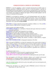
Figure 11. Observed iodide, tritium and sodium in the borehole fluid during an in-situ diffusion experiment in Opalinus Clay<br />
(symbols) and model calculated concentrations (lines) in Mont Terri experiment. The dotted lines stem from a model in<br />
which tritium, iodide and sodium have the same tortuosity. The full line for iodide results when the tortuosity is increased by<br />
1.2. The full line for 22 Na is obtained with a 1.5 times smaller tortuosity than of tritium (<strong>Appelo</strong> and Wersin, 2007).<br />
The tortuosity of iodide is higher than of tritium. It can be explained by the heterogeneous<br />
distribution of clay minerals which creates a spatially variable diffuse double layer that blocks<br />
transport of the anions in pore constrictions where cations and tritium can continue to diffuse. The<br />
tortuosity of 22 Na + is smaller than of tritium. This is more difficult to explain, and may be a result of<br />
diffusion through the interlayer space of swelling clay minerals, or perhaps of surface diffusion of<br />
exchangeable cations.<br />
6. CONCLUSIONS<br />
Version 2.13 of the PHREEQC hydrogeochemical code was extended with multicomponent<br />
diffusion and diffuse double layer diffusion for comprehensive modeling of transport in clays. The<br />
code can handle laboratory and in-situ diffusion experiments in a way not possible hitherto. Examples<br />
of multicomponent diffusion were discussed, showing 1) uphill diffusion as a result of different<br />
diffusion speeds of individual ions, a process that cannot be explained by Fickian diffusion, 2)<br />
precipitation reactions that can only be modeled correctly with kinetic rates, 3) precipitation of<br />
scheelite in a laboratory diffusion experiment, and 4) an in-situ diffusion experiment in Opalinus Clay<br />
where diffusion data of tritium, 22 Na + and I - were modeled altogether in an elliptical grid.<br />
Acknowledgements<br />
The PHREEQC input files for the cases presented are available on request to appt@xs4all.nl. Paul Wersin aroused my<br />
interest in the Opalinus Clay experiments, and so incented the adaptations of PHREEQC reported here.<br />
REFERENCES<br />
<strong>Appelo</strong>, C.A.J. and Postma, D. (2005): Geochemistry, groundwater and pollution, 2 nd ed. Balkema,<br />
Leiden, 649 pp.<br />
Water pollution in natural porous media; Candela, L., Vadillo, I., Aagaard, P., Eds.; Instituto<br />
Geológico de España: Madrid, 2007 12
<strong>Appelo</strong>, C.A.J. and Wersin, P. (2007): Multicomponent diffusion modeling in clay systems with<br />
application to the diffusion of tritium, iodide and sodium in Opalinus Clay. Environ. Sci. Technol.<br />
41, 5002-5007.<br />
Ben-Yaakov, S. (1972): Diffusion of seawater ions into dilute solution. Geochim. Cosmochim. Acta,<br />
36: 1396-1406.<br />
Boudreau, B.P., Meysman, F.J.R., and Middelburg, J.J. (2004): Multicomponent ionic diffusion in<br />
porewaters: Coulombic effects revisited. Earth Planet. Sci. Lett., 222: 653-666.<br />
Cussler, E.L. (1984): Diffusion - mass transfer in fluid systems. Cambridge UP, 525 pp.<br />
Lichtner, P.C. (1995): Principles and practice of reactive transport modeling. Mat. Res. Soc. Symp.<br />
Proc., 353: 117-130.<br />
Parkhurst, D.L. and <strong>Appelo</strong>, C.A.J. (1999): User’s guide to PHREEQC (version 2). U.S. Geol. Surv.<br />
Water Resour. Inv. Rep. 99-4259, 312 pp.<br />
Pina, C.M., Fernández-Díaz, L. and Astilleros, J.M. (2000): Nucleation and growth of scheelite in a<br />
diffusing-reacting system. Cryst. Res. Technol., 35: 1015-1022.<br />
Prieto, M., Putnis, A. and Fernández-Díaz, L. (1990): Factors controlling the kinetics of<br />
crystallization: supersaturation evolution in a porous medium. Geol. Mag., 127: 485-495.<br />
Prieto, M., Fernández-González, A., Putnis, A. and Fernández-Díaz, L. (1997): Nucleation, growth,<br />
and zoning phenomena in crystallizing (Ba, Sr)CO 3 , Ba(SO 4 , CrO 4 ), (Ba, Sr)SO 4 and (Cd, Ca)CO 3<br />
solid solutions from aqueous solutions. Geochim. Cosmochim. Acta, 61: 3383-3397.<br />
Robinson, R.A. and Stokes, R.H. (1959): Electrolyte solutions: the measurement and interpretation of<br />
conductance, chemical potential and diffusion in solutions of simple electrolytes. Butterworths,<br />
London.<br />
Sato, H., Ashida, T., Kohara, Y., Yui, M. and Sasaki, M. (1992): Effect of dry density on diffusion of<br />
some radionuclides in compacted sodium bentonite. J. Nucl. Sci. Technol., 29: 873-882.<br />
Van Loon, L.R., Soler, J.M., Müller, W. and Bradbury, M.H. (2004): Anisotropic diffusion in layered<br />
argillaceous formations: a case study with Opalinus clay. Environ. Sci. Technol., 38: 5721-5728.<br />
Vinograd, J.R. and McBain, J.W. (1941): Diffusion of electrolytes and of the ions in their mixtures. J.<br />
Am. Chem. Soc., 63: 2008-2015.<br />
Wersin, P., Van Loon, L.R., Soler, J.M., Yllera, A., Eikenberg, J., Gimmi, Th., Hernán, P. and<br />
Boisson, J.Y. (2004): Long-term diffusion experiment at Mont Terri: first results from field and<br />
laboratory data. Applied Clay Sci., 26: 123-135.<br />
Water pollution in natural porous media; Candela, L., Vadillo, I., Aagaard, P., Eds.; Instituto<br />
Geológico de España: Madrid, 2007 13