Break date estimation for models with deterministic structural change

More documents

Recommendations

Info

Perron, P. and Zhu, X. (2005). Structural breaks with deterministic and stochastic trends. Journal of Econometrics 129, 65{119. Saygnsoy, O. and Vogelsang, T.J. (2011). Testing for a shift in trend at an unknown date: a xed-b analysis of heteroskedasticity autocorrelation robust OLS based tests. Econometric Theory 27, 992{1025. Stock, J.H. and Watson, M.W. (1996). Evidence on structural instability in macroeconomic time series relations. Journal of Business and Economic Statistics 14, 11{30. Stock, J.H. and Watson, M.W. (1999). A comparison of linear and nonlinear univariate models for forecasting macroeconomic time series. Engle, R.F. and White, H. (eds.), Cointegration, Causality and Forecasting: A Festschrift in Honour of Clive W.J. Granger, Oxford: Oxford University Press, 1{44. Stock, J. and Watson, M.W. (2005). Implications of dynamic factor analysis for VAR models, NBER Working Paper #11467. Vogelsang, T.J. (1998). Testing for a shift in mean without having to estimate serialcorrelation parameters. Journal of Business and Economic Statistics 16, 73{80. Yang, J. (2012). Break point estimators for a slope shift: levels versus rst dierences. Econometrics Journal 15, 154{169. 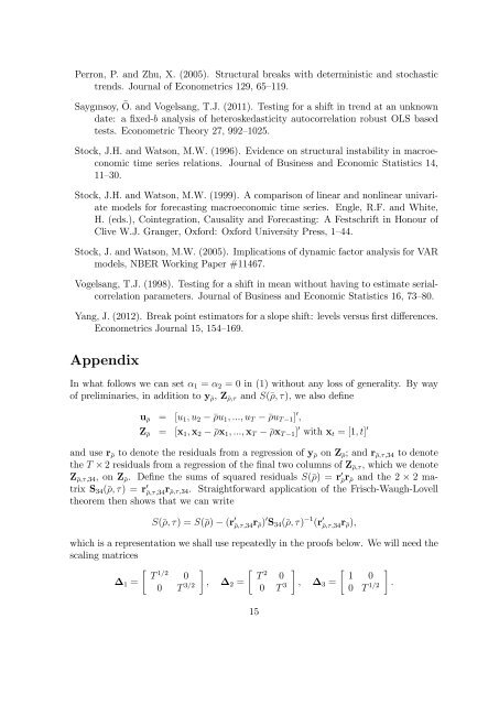Appendix In what follows we can set 1 = 2 = 0 in (1) without any loss of generality. By way of preliminaries, in addition to y , Z ; and S(; ), we also dene u = [u 1 ; u 2 u 1 ; :::; u T u T 1 ] 0 ; Z = [x 1 ; x 2 x 1 ; :::; x T x T 1 ] 0 with x t = [1; t] 0 and use r to denote the residuals from a regression of y on Z ; and r ;;34 to denote the T 2 residuals from a regression of the nal two columns of Z ; , which we denote Z ;;34 , on Z . Dene the sums of squared residuals S() = r 0 r and the 2 2 matrix S 34 (; ) = r 0 ;;34r ;;34 . Straightforward application of the Frisch-Waugh-Lovell theorem then shows that we can write S(; ) = S() (r 0 ;;34r ) 0 S 34 (; ) 1 (r 0 ;;34r ); which is a representation we shall use repeatedly in the proofs below. We will need the scaling matrices T 1=2 0 T 2 0 1 0 1 = 0 T 3=2 ; 2 = 0 T 3 ; 3 = 0 T 1=2 : 15
The following preliminary lemmas are also used. The terms involved in Lemma 1 do not involve any stochastic components and the proofs are entirely straightforward and are therefore not presented. Lemma 1 (i) For jj < 1 1 1 Z 0 Z 1 1 ! (1 ) 2 1 1=2 1=2 1=3 1 1 Z 0 Z ;;34 1 1 ! (1 ) 2 ; (9) (1 ) (1 ) 2 =2 (1 2 )=2 (1 ) 2 (2 + )=6 ; (10) 1 1 S 34 (; ) 1 1 ! (1 ) 2 B 2 (): (11) where B 2 () is as dened in Theorem 1. (ii) For = 1 1 3 Z 0 1Z 1 1 3 ! 1 3 Z 0 1Z 1;;34 1 3 ! 1 3 S 34 (1; ) 1 3 ! 1 0 ; (12) 0 1 0 0 ; (13) 0 1 1 0 : (14) 0 (1 ) Lemma 2 Under Assumption I(0), (i) for jj < 1 T 1 S() ) !2 " 1 2 (1 + 2 2); (15) 1 1 r 0 ;;34r ) (1 ) 2 ! u fA( 0 1; 0 2; ; ) B 1 ()C( 0 1; 0 2; )g (16) where A( 0 1; 0 2; ; ), B 1 () and C( 0 1; 0 2; ) are as dened in Theorem 1, (ii) for = 1 r 0 1;;34r 1 = T 1 S(1) ) 2!2 " 1 + ; (17) u T +1 + o(1): (18) u T u T + (1 )u 1 Proof of Lemma 2 (i) Write T 1 S() = T 1 y 0 y T 1 y 0 Z 1 1 [ 1 1 Z 0 Z 1 1 ] 1 1 1 Z 0 y : 16
Page 1 and 2: Break date estimation for models wi
Page 3 and 4: 1 Introduction The recent literatur
Page 5 and 6: the appropriate Pitman drifts for t
Page 7 and 8: Figure 1 provides histograms of the
Page 9 and 10: where D 2 = f 0 ; 1g. 4 To examine
Page 11 and 12: Now d( 2 2) = 2( ) d and so arg min
Page 13 and 14: Table 1 concerns the case of I(0),
Page 15: Newton-type minimization methods. M
Page 19 and 20: i.e. (16). (ii) Write and T 1 S(1)
Page 21 and 22: and using (9) these results give (2
Page 23 and 24: Since (1 ) 2 ! 2 u appears only as
Page 25 and 26: Table 1. Probability of break fract
Page 35 and 36: ˆτ 1 ˆτ 1 (a) κ 1 = 1, κ 2 =

Break date estimation for models with deterministic structural change

Create successful ePaper yourself

Delete template?

Save as template?