Break date estimation for models with deterministic structural change

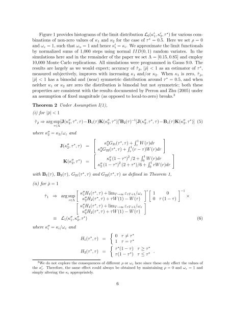
Figure 1 provides histograms of the limit distribution L 0 ( 0 1; 0 2; ) for various combinations
of non-zero values of 1 and 2 for the case of = 0:5. Here we set = 0
and ! " = 1, such that ! u = 1 and hence 0 i = i . We approximate the limit functionals
by normalized sums of 1,000 steps using normal IID(0; 1) random variates. In the
simulations here and in the remainder of the paper we set = [0:15; 0:85] and employ
10,000 Monte Carlo replications. All simulations were programmed in Gauss 9.0. The
results are largely as we would expect; accuracy of ^ , jj < 1 as an estimator of ,
measured subjectively, improves with increasing 1 and/or 2 . When 1 is zero, ^ ,
jj < 1 has a bimodal and (near) symmetric distribution around = 0:5, and when
neither 1 or 2 are zero the distribution is bimodal but not symmetric; both these
properties are consistent with the results documented by Perron and Zhu (2005) under
an assumption of xed magnitude (as opposed to local-to-zero) breaks. 3
Theorem 2 Under Assumption I(1),
(i) for jj < 1
^ ) arg sup[J( 00
2; ; ) B 1 ()K( 00
2; )] 0 B 2 () 1 [J( 00
2; ; ) B 1 ()K( 00
2; )] (5)
2
where 00
2 = 2 =! " and
J( 00
2; ; ) =
K( 00
2; ) =
"
"
00
2G 21 ( ; ) + R #
1
W (r)dr
2G 22 ( ; ) + R 1
(r )W (r)dr
00
00
2 (1 ) 2 =2 + R #
1
W (r)dr
0
00
2 (1 ) 2 (2 + )=6 + R 1
rW (r)dr 0
with B 1 (), B 2 (), G 21 ( ; ) and G 22 ( ; ) as dened in Theorem 1,
(ii) for = 1
00
^ 1 ) arg sup 1H 1 ( 0 1
; ) + lim T !1 " T +1 =! " 1 0
2 00
2H 2 (
; ) + W (1) W () 0 (1 )
00
1H 1 ( ; ) + lim T !1 " T +1 =! "
00
2H 2 ( ; ) + W (1) W ()
L 1 ( 00
1; 00
2; ) (6)
where 00
i = i =! " and
H 1 ( ; ) =
H 2 ( ; ) =
0 6=
1 =
(1 )
(1 ) :
3 We do not explore the consequences of dierent or ! " here since these only eect the values of
the 0 i . Therefore, the same eect could always be obtained by maintaining = 0 and ! " = 1 and
simply altering the i appropriately.
6