short-term travel time prediction using a neural network
short-term travel time prediction using a neural network
short-term travel time prediction using a neural network

Create successful ePaper yourself
Turn your PDF publications into a flip-book with our unique Google optimized e-Paper software.
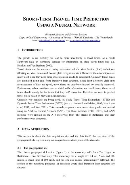
SHORT-TERM TRAVEL TIME PREDICTION<br />
USING A NEURAL NETWORK<br />
Giovanni Huisken and Eric van Berkum<br />
Dept. of Civil Engineering - University of Twente - 7500 AE Enschede - The Netherlands<br />
E-mail: g.huisken@ctw.utwente.nl and e.c.vanberkum@ctw.utwente.nl<br />
1 INTRODUCTION<br />
The growth in car mobility has lead to more uncertainty in <strong>travel</strong> <strong>time</strong>s. As a result<br />
cardrivers have an increasing demand for information on these <strong>travel</strong> <strong>time</strong>s (see e.g.<br />
Huisken and Van Berkum, 2000).<br />
Travel <strong>time</strong>s can be measured <strong>using</strong> automated vehicle identification (AVI) techniques<br />
(floating car data, automated license plate recognition, etc.). However, these techniques are<br />
rarely used since they need large investments in roadside equipment. Currently <strong>travel</strong> <strong>time</strong>s<br />
are estimated <strong>using</strong> data from inductive loop detectors. Since loop detectors yield spot<br />
measurements of flow and speed, <strong>travel</strong> <strong>time</strong>s can only be estimated, not actually measured.<br />
Furthermore, when cardrivers are provided with information on <strong>travel</strong> <strong>time</strong>s, these <strong>travel</strong><br />
<strong>time</strong>s should ideally be the <strong>time</strong>s that they will encounter. Therefore we need to predict<br />
<strong>travel</strong> <strong>time</strong>s, based on previous measurements.<br />
Currently two methods are being used, i.e. Static Travel Time Estimations (STTE) and<br />
Dynamic Travel Time Estimations (DTTE) (see e.g. Hounsell and Ishtiaq, 1997; Van Arem<br />
et al, 1997; and Zee, 2001). This research proposes a new <strong>travel</strong> <strong>time</strong> <strong>prediction</strong> method<br />
<strong>using</strong> an Artificial Neural Network (ANN). The three methods STTE, DTTE, and ANN<br />
methods were applied on the A13 motorway from The Hague to Rotterdam and their<br />
performance was compared.<br />
2 DATA ACQUISITION<br />
This section is about the data acquisition site and the data itself. An overview of the<br />
geographical site is given along with a quantitative description of the data sets.<br />
2.1 The geographical site<br />
The chosen geographical location (figure 1) is the motorway A13 from The Hague to<br />
Rotterdam – one direction only. This motorway has a length of 11.4 km, 5 on- and offramps,<br />
a speed limit of 100 km/h, and has one gas station (approximately halfway). The<br />
section of the motorway possesses 21 locations where dual induction loop detectors are<br />
situated.
Figure 1. The motorway section from The Hague to Rotterdam.<br />
2.2 Data sets description<br />
In this contribution two main issues will be addressed. First a method is selected that yields<br />
the best <strong>travel</strong> <strong>time</strong> estimate <strong>using</strong> inductive loop data. Second, three methods to predict<br />
<strong>travel</strong> <strong>time</strong>s are being compared. For the first part two data sets have been acquired: one<br />
licence plate recognition set (Delft-Noord/Nootdorp [km 7.3 post] – Rotterdam-Overschie<br />
[km 17.55 post]) and one through the dual induction loop detectors with the MARI [More<br />
Applicatie Routekeuze Informatie] system. The licence plate recognition set was acquired by<br />
<strong>time</strong> and licence plate registration of passing red vehicles at the starting and re-identification<br />
point and subsequent subtraction produced <strong>travel</strong> <strong>time</strong>s. The collection took place on<br />
October 8 th and 9 th 1996: 07:00 – 09:30 and 15:30 – 18:30 and on October 11 th 1996:<br />
15:00 – 18:45. During this period, also inductive loop data for the 21 locations were<br />
collected, containing flow and speed on a one-minute basis.<br />
For the second part, i.e. the comparison of the three <strong>prediction</strong> methods, loop data was<br />
collected from November 11 th 1996 – February 23 rd 1997. The set also contains 1-minute<br />
aggregated data from loop detectors containing information on flow and speed.<br />
3 METHODS AND MODEL DEVELOPMENT<br />
3.1 Estimation of <strong>travel</strong> <strong>time</strong>s <strong>using</strong> inductive loop data<br />
From Bovy and Thijs (2000) five algorithms (RT0 - RT4) were selected and tested for the<br />
estimation of <strong>travel</strong> <strong>time</strong>s <strong>using</strong> loop detector data (table 1). The estimates these methods<br />
yield were compared with the actual measured <strong>travel</strong> <strong>time</strong>s <strong>using</strong> license plate recognition<br />
RT_M_AVG (figure 2).<br />
Table 1. Travel <strong>time</strong> estimation methods.<br />
Link method Route method Smoothing<br />
Speed Mass balance Static Dynamic Input Output<br />
RT0 x x x x x<br />
RT1 x x x x<br />
RT2 x x x<br />
RT3 x x x<br />
RT4 x x
15<br />
13<br />
11<br />
RT4<br />
9<br />
RT3<br />
Travel <strong>time</strong> [m]<br />
7<br />
5<br />
15<br />
16<br />
17<br />
18<br />
19<br />
RT2<br />
RT1<br />
RT0<br />
RT_M _A V G<br />
Time of day<br />
Figure 2. Estimated <strong>travel</strong> <strong>time</strong>s by method.<br />
RT4 gave the best results (an average error of 23.0 seconds on a mean <strong>travel</strong> <strong>time</strong> of 8<br />
minutes and 46 seconds – after shifting). Since for the training of the <strong>neural</strong> <strong>network</strong>, as<br />
well as for the comparison of the three <strong>prediction</strong> methods only inductive loop data are<br />
available and no actual <strong>travel</strong> <strong>time</strong> measurements, RT4 is applied to construct a dataset of<br />
<strong>travel</strong> <strong>time</strong>s.<br />
3.2 Prediction <strong>using</strong> static <strong>travel</strong> <strong>time</strong> estimation<br />
STTE uses last-known link <strong>travel</strong> <strong>time</strong>s and sums them. Links (L) are defined as the<br />
distance between two consecutive dual induction loops. Suppose a vehicle enters a specific<br />
route (number of links = k) at <strong>time</strong> t = T 0 . The most recent recorded loop speeds v n (T 0 ), (n =<br />
1..k), are assigned to half of the link before and after the specific loop location. STTE<br />
becomes:<br />
STTE T0<br />
= L k −1<br />
2<br />
− L 1<br />
2 ⋅v 1 ( T 0 ) + ⎛ L n+1<br />
− L n−1<br />
⎞<br />
⎜ ⎟ + L k<br />
− L<br />
∑<br />
k −1<br />
() 1<br />
n= 2 ⎝ 2⋅ v n ( T 0 ) ⎠ 2 ⋅ v k ( T 0 )<br />
So, link <strong>travel</strong> <strong>time</strong>s are assumed fixed as of the moment that the vehicle enters the route<br />
(T 0 ).<br />
3.3 Prediction <strong>using</strong> dynamic <strong>travel</strong> <strong>time</strong> estimation<br />
DTTE at <strong>time</strong> T 0 can only be estimated by historical reconstruction and is done iteratively.<br />
Suppose at T 0 vehicle 2 enters the motorway and vehicle 1 is the last vehicle that left the<br />
motorway. From the recorded speed data the <strong>travel</strong> <strong>time</strong> that vehicle 1 did encounter can be<br />
reconstructed. Now DTTE uses this <strong>travel</strong> <strong>time</strong> as a <strong>prediction</strong> for vehicle 2.
3.4 Prediction <strong>using</strong> artificial <strong>neural</strong> <strong>network</strong>s<br />
ANNs are based upon biological <strong>neural</strong> <strong>network</strong>s by mimicking their architectural structure<br />
and information processing in a simplified manner. They both consist of processing<br />
elements called neurons that are highly interconnected making the <strong>network</strong>s parallel<br />
information processing systems. They are capable of tasks such as pattern recognition,<br />
perception and motor control that are considered poorly performed by conventional linear<br />
processing. These parallel systems are also known to be robust and to have the capability to<br />
capture highly non-linear mappings between input and output. ANN applications in<br />
transport can be found in e.g. Dougherty (1995) and Huisken (1998 and 2001).<br />
Here Multi Layer Feedforward (MLF) <strong>neural</strong> <strong>network</strong>s were used. The MLF is a supervised<br />
learning <strong>network</strong> meaning that during the training phase all inputs are mapped on desired<br />
outputs. The error, i.e. the difference between the actual and the desired output, is a criterion<br />
that is used to adjust the weights of the neurons iteratively so that the total error of all inputoutput<br />
pairs is minimised. The algorithm responsible for this method is called the learning<br />
rule. More comprehensive information on MLF <strong>neural</strong> <strong>network</strong>s can be found in any<br />
textbook on ANNs.<br />
MLF <strong>network</strong>s will be trained with the most accurate <strong>travel</strong> <strong>time</strong>s as targets. The number of<br />
input variables is: 21 (induction loops) * 2 (quantities: speed and intensity) + 1 (<strong>time</strong> of day)<br />
= 43. This high number of inputs resulted in <strong>time</strong> consuming training phases so preprocessing<br />
was used to cut the input down to 12 inputs. The data set was divided into 3<br />
equally sized subsets (for cross-validation purposes) where one subset was used as test set to<br />
find the optimum number of hidden neurons and epochs (training cycles) and to prevent the<br />
MLF <strong>network</strong> from overfitting.<br />
4 RESULTS & CONCLUSIONS<br />
The <strong>prediction</strong>s of the three methods were compared with the <strong>travel</strong> <strong>time</strong>s de<strong>term</strong>ined by<br />
RT4. Travel <strong>time</strong> <strong>prediction</strong> becomes interesting when free flow conditions no longer hold.<br />
Therefore <strong>prediction</strong> was only executed when <strong>travel</strong> <strong>time</strong>s exceeded 500 seconds (i.e.<br />
average speed under 82 km/h). To compare the method’s performances several measures of<br />
error were de<strong>term</strong>ined (see formula 2): the Mean Relative Error (MRE) [%], the Mean<br />
Absolute Relative Error (MARE) [%], the Mean Time Error (MTE) [seconds], the Mean<br />
Absolute Time Error (MATE) [seconds], and R-squared.<br />
MRE =<br />
t ˆ n<br />
− t<br />
∑<br />
n<br />
MARE =<br />
n n ⋅ ˆ t n<br />
t ˆ n<br />
− t<br />
∑<br />
n<br />
MTE =<br />
n n ⋅ ˆ t n<br />
∑ ˆ t n<br />
− t n<br />
n<br />
MATE = ∑ t ˆ n<br />
− t n<br />
n<br />
(2)<br />
where n is the number of cases, t ˆ n<br />
is the <strong>travel</strong> <strong>time</strong> to be predicted (target value from RT4),<br />
and t n<br />
is the <strong>travel</strong> <strong>time</strong> generated by the model.<br />
n<br />
n
The results are given in table 2 that shows that MLF significantly outperforms DTTE, which<br />
in turn significantly outperforms STTE. The MRE values are also classified into 5%-error<br />
intervals and from this can be concludes that roughly two-thirds, a half, and one-third of the<br />
<strong>prediction</strong> cases fall in the [-5%, 5%] error domain (between the 2 vertical lines) for MLF,<br />
DTTE, and STTE, respectively (figure 4).<br />
Table 2. MRE, MARE, MTE, MATE and R-squared results.<br />
MRE [%] MARE [%] MTE [sec] MATE [sec] R-squared<br />
STTE 1.06 10.7 -2.30 79.5 0.816<br />
DTTE -1.71 6.91 -7.75 55.0 0.874<br />
MLF -0.249 4.61 -0.107 35.1 0.957<br />
STTE DTTE MLF<br />
35<br />
30<br />
25<br />
20<br />
15<br />
10<br />
5<br />
0<br />
Figure 4. Distribution of MRE.<br />
REFERENCES<br />
Bovy P.H.L. and Thijs R. (2000). Estimators of <strong>travel</strong> <strong>time</strong> for road <strong>network</strong>s, new<br />
developments, evaluation results, and applications, Delft University of Technology.<br />
Dougherty M.S. (1995). A review of <strong>neural</strong> <strong>network</strong>s applied to transport. Transpn. Res.-C,<br />
3(4), pp 247 – 260.<br />
Hounsell N.B. and Ishtiaq S. (1997). Journey <strong>time</strong> forecasting for dynamic route guidance<br />
systems in incident conditions. Int. J. Forecasting, 13(1), pp 33 – 42.
Huisken G. (1998). Literature review: <strong>neural</strong> <strong>network</strong> applications in traffic and transport.<br />
Research report: University of Twente, The Netherlands.<br />
Huisken G. (2001). Short-<strong>term</strong> forecasting of traffic flow on freeways. Proc. of the 9 th<br />
World Conference on Transport Research, July 2001, Seoul, Korea.<br />
Huisken G. and Van Berkum E.C. (2000). DAB in the Netherlands? Proc. of the 8 th Meeting<br />
of the Euro Working Group Transportation EWGT, September 2000, Rome, Italy.<br />
Van Arem B., Van Der Vlist M.J.M., Muste M. and Smulders S.A. (1997). Travel <strong>time</strong><br />
estimation in the GERDIEN project. Int. J. Forecasting, 13(1), pp 73 – 85.<br />
Zee J.C. (2001). Oude reistijden actueel. M.Sc. report, University of Twente, Enschede, The<br />
Netherlands [In Dutch].