CALIBRATION OF HEADWAY DISTRIBUTIONS

Capacity (veh/h)
1500
1400
1300
1200
1100
1000
900
ML
VR
D +
D -
W 2
A 2
obs
800
700
600
500
0 200 400 600 800 1000 1200
Volume (veh/h)
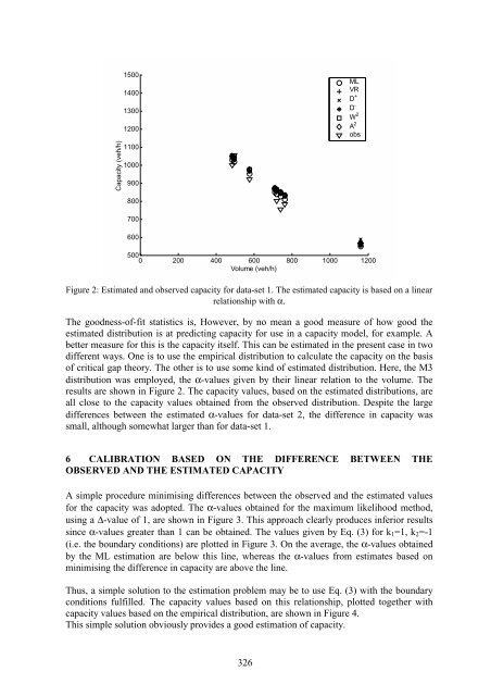
Figure 2: Estimated and observed capacity for data-set 1. The estimated capacity is based on a linear
relationship with α.
The goodness-of-fit statistics is, However, by no mean a good measure of how good the
estimated distribution is at predicting capacity for use in a capacity model, for example. A
better measure for this is the capacity itself. This can be estimated in the present case in two
different ways. One is to use the empirical distribution to calculate the capacity on the basis
of critical gap theory. The other is to use some kind of estimated distribution. Here, the M3
distribution was employed, the α-values given by their linear relation to the volume. The
results are shown in Figure 2. The capacity values, based on the estimated distributions, are
all close to the capacity values obtained from the observed distribution. Despite the large
differences between the estimated α-values for data-set 2, the difference in capacity was
small, although somewhat larger than for data-set 1.
6 CALIBRATION BASED ON THE DIFFERENCE BETWEEN THE
OBSERVED AND THE ESTIMATED CAPACITY
A simple procedure minimising differences between the observed and the estimated values
for the capacity was adopted. The α-values obtained for the maximum likelihood method,
using a ∆-value of 1, are shown in Figure 3. This approach clearly produces inferior results
since α-values greater than 1 can be obtained. The values given by Eq. (3) for k 1 =1, k 2 =-1
(i.e. the boundary conditions) are plotted in Figure 3. On the average, the α-values obtained
by the ML estimation are below this line, whereas the α-values from estimates based on
minimising the difference in capacity are above the line.
Thus, a simple solution to the estimation problem may be to use Eq. (3) with the boundary
conditions fulfilled. The capacity values based on this relationship, plotted together with
capacity values based on the empirical distribution, are shown in Figure 4.
This simple solution obviously provides a good estimation of capacity.