CALIBRATION OF HEADWAY DISTRIBUTIONS
CALIBRATION OF HEADWAY DISTRIBUTIONS
CALIBRATION OF HEADWAY DISTRIBUTIONS

You also want an ePaper? Increase the reach of your titles
YUMPU automatically turns print PDFs into web optimized ePapers that Google loves.
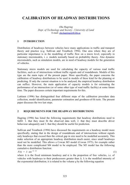
<strong>CALIBRATION</strong> <strong>OF</strong> <strong>HEADWAY</strong> <strong>DISTRIBUTIONS</strong><br />
Ola Hagring<br />
Dept. of Technology and Society - University of Lund<br />
E-mail: ola.hagring@tft.lth.se<br />
1 INTRODUCTION<br />
Distribution of headways between vehicles have many applications in traffic and transport<br />
theory and practice (e.g. Sullivan and Troutbeck 1994). One area where they are of<br />
particular importance is in the modelling of traffic flow on a micro level, especially in<br />
stationary micromodels, i. e. models normally based on probability theory. Also dynamic<br />
micromodels, such as simulation models, are in need of headway models for the generation<br />
of vehicles.<br />
Stationary micro models are used for calculating the capacity of various road traffic<br />
facilities, such as of intersections without traffic signals and of roundabouts. Models of this<br />
type are the main topic of the present paper. More specifically, the paper concerns the<br />
calibration of headway distributions to be used in models of these kind for the planning or<br />
predicting. If only the current situation is to be analysed, the empirical headway distribution<br />
can suffice. However, the main application of capacity models is for estimating the<br />
performance of an intersection (or of some other type of road traffic facility) at some future<br />
time. The paper discusses certain important requirements for this.<br />
Luttinen (1996) has distinguished four different steps of the calibration procedure data<br />
collection, model identification, parameter estimation and goodness-of-fit tests. The present<br />
paper discusses the two last steps.<br />
2 REQUIREMENTS FOR THE <strong>HEADWAY</strong> <strong>DISTRIBUTIONS</strong><br />
Hagring (1996) has listed the following requirements that headway distributions need to<br />
fulfil: 1. that they must fit the observed data well, 2. that they must describe driver<br />
behaviour adequately and 3. that they should be useful for prediction.<br />
Sullivan and Troutbeck (1994) have discussed the requirements on a headway model more<br />
specifically, stating that in the design of roundabouts and of intersections without signals<br />
only headways that exceed then the critical gap in size need to be modelled accurately. This<br />
make selection of an appropriate headway distribution much easier, since small headways<br />
need not be modelled. This allows a Cowan M3 model (Cowan 1975), for example rather<br />
than the more complicated M4 model to be employed. The M3 model has the following<br />
cumulative distribution function:<br />
F(t) = 1- αe − ( t −∆)<br />
(1)<br />
where ∆ is the fixed minimum headway and α is the proportion of free vehicles, i.e. of<br />
vehicles with headways to their predecessors greater than ∆. λ is the modified intensity of<br />
the exponential distribution; it is related to the volume q by the following equation
λ= qα<br />
1− q∆ . (2)<br />
The M3 distribution is theoretically capable of fulfilling requirement 2. above because of<br />
the parameters ∆ and α, although not in the case of small headways. The modelling of small<br />
headways by a fixed value instead of by a complete distribution is based on a simplified<br />
model of driver behaviour.<br />
Requirements 1. and 3. are closely connected, in that it may be possible to fit a given<br />
headway distribution to a number of different observed headways. If one has a number of<br />
independent data sets, it may also be possible to fit a distribution to each of them. However,<br />
as Hagring (1996, 1998) has noted, if the variation in the estimated parameters, i.e. α and ∆,<br />
in a particular headway distribution cannot be related to some independent variable,<br />
normally the volume, the distribution is not useful for prediction purposes.<br />
3 TECHNIQUES FOR PARAMETER ESTIMATION<br />
Different methods can be used to obtain the parameter values in the M3 distribution. Three<br />
methods commonly employed are the method of moments, the maximum-likelihood method<br />
and the least squares method.<br />
4 PARAMETER ESTIMATION<br />
Hagring (1998) employed the three estimation methods just mentioned for estimating the<br />
parameters of the M3 distribution so as to obtain some relation between α and the volume<br />
that could be of use. ∆ was fixed and regression analysis was used to derive a linear<br />
relationship between α and q involving the parameters k 1 and k 2<br />
α = k1+ k2q<br />
(3)<br />
The ∆-values can be based on behavioural assumptions or, as in the present case, be taken as<br />
the inverse of the maximum flow in one lane during stationary conditions. Two data-sets<br />
containing headways from roundabouts with two circulating lanes were employed.
1<br />
0.9<br />
0.8<br />
0.7<br />
ML<br />
VR+<br />
D-<br />
D 2<br />
W2<br />
A<br />
0.6<br />
α<br />
0.5<br />
0.4<br />
0.3<br />
0.2<br />
0.1<br />
0<br />
0 200 400 600 800 1000 1200<br />
Volume (veh/h)<br />
Figure 1: Estimation of α by use of various goodness-of-fit measures and the maximum likelihood<br />
method (ML), for data-set 1.<br />
The result of the maximum likelhood estimation of α when ∆ was fixed to 1 s. is shown in<br />
Figure 1. Although some variation is still present there is a clear dependency of α on q.<br />
In an optimal model for α, α should be equal to 0 when the volume is at capacity and to 1<br />
when the volume is 0, i.e. k 1 should be equal to 1 and k 2 should be equal to the minimum<br />
headway. None of the estimated models were optimal. The method of moments appeared to<br />
give the most accurate results.<br />
5 IMPROVING THE FITTING <strong>OF</strong> A DISTRIBUTION<br />
If parameter estimation is performed by use of the maximum-likelihood method, it may be<br />
possible to improve the fitting of the estimated distribution such as by further minimising<br />
the variance of the residuals. Troutbeck (1997) has described a method of this sort In the<br />
present study, a number of other goodness-of-fit measures were also investigated: the<br />
supremum statistics, D + and D - ; the Cramer-von Mises statistic termed<br />
W 2 ; and the Anderson-Darling statistic termed A 2 . The formulas, including those used for<br />
computing purposes are given by Stephens (1986). Figure 1 shows the estimated α-values.<br />
These are quite close to each other, except that for data-set 2 (not shown) the α-values<br />
differed considerably. This was due to the traffic flow for some of the subsets being<br />
markedly disturbed by traffic signals.
Capacity (veh/h)<br />
1500<br />
1400<br />
1300<br />
1200<br />
1100<br />
1000<br />
900<br />
ML<br />
VR<br />
D +<br />
D -<br />
W 2<br />
A 2<br />
obs<br />
800<br />
700<br />
600<br />
500<br />
0 200 400 600 800 1000 1200<br />
Volume (veh/h)<br />
Figure 2: Estimated and observed capacity for data-set 1. The estimated capacity is based on a linear<br />
relationship with α.<br />
The goodness-of-fit statistics is, However, by no mean a good measure of how good the<br />
estimated distribution is at predicting capacity for use in a capacity model, for example. A<br />
better measure for this is the capacity itself. This can be estimated in the present case in two<br />
different ways. One is to use the empirical distribution to calculate the capacity on the basis<br />
of critical gap theory. The other is to use some kind of estimated distribution. Here, the M3<br />
distribution was employed, the α-values given by their linear relation to the volume. The<br />
results are shown in Figure 2. The capacity values, based on the estimated distributions, are<br />
all close to the capacity values obtained from the observed distribution. Despite the large<br />
differences between the estimated α-values for data-set 2, the difference in capacity was<br />
small, although somewhat larger than for data-set 1.<br />
6 <strong>CALIBRATION</strong> BASED ON THE DIFFERENCE BETWEEN THE<br />
OBSERVED AND THE ESTIMATED CAPACITY<br />
A simple procedure minimising differences between the observed and the estimated values<br />
for the capacity was adopted. The α-values obtained for the maximum likelihood method,<br />
using a ∆-value of 1, are shown in Figure 3. This approach clearly produces inferior results<br />
since α-values greater than 1 can be obtained. The values given by Eq. (3) for k 1 =1, k 2 =-1<br />
(i.e. the boundary conditions) are plotted in Figure 3. On the average, the α-values obtained<br />
by the ML estimation are below this line, whereas the α-values from estimates based on<br />
minimising the difference in capacity are above the line.<br />
Thus, a simple solution to the estimation problem may be to use Eq. (3) with the boundary<br />
conditions fulfilled. The capacity values based on this relationship, plotted together with<br />
capacity values based on the empirical distribution, are shown in Figure 4.<br />
This simple solution obviously provides a good estimation of capacity.
1.4<br />
1.2<br />
ML<br />
Cap<br />
Eq. (3), k 1<br />
=1, k 2<br />
=-1<br />
1<br />
0.8<br />
α<br />
0.6<br />
0.4<br />
0.2<br />
0<br />
0 500 1000 1500 2000 2500 3000 3500 4000<br />
Volume (veh/h)<br />
Figure 3: Values of α, as estimated by the ML method and by minimising the difference in capacity<br />
between the observed and the estimated distribution.<br />
1400<br />
1300<br />
Eq. (2), k =1, k =-1<br />
1 2<br />
Observed capacity<br />
Capacity (veh/h)<br />
1200<br />
1100<br />
1000<br />
900<br />
800<br />
700<br />
600<br />
500<br />
0 200 400 600 800 1000 1200<br />
Volume (veh/h)<br />
Figure 4: Observed capacity and capacity based on Eq. (2) with boundary values fulfilled.<br />
It can thus be concluded that the M3 distribution is robust and that in most cases there is no<br />
need for extensive calibration, using Eq. (3) with the boundary conditions fulfilled being
good enough. There is the possibility however, that fitting some other distributions could<br />
yield better results.<br />
REFERENCES<br />
Cowan, R. J. (1975). Useful headway models. Transportation Research 9(6), pp. 371-375.<br />
Hagring, O. (1996). The use of the Cowan M3 distribution for modelling roundabout flow.<br />
Traffic Engineering & Control 37(5), pp. 328-332.<br />
Hagring, O. (1998). Vehicle-vehicle interactions at roundabouts and their implications for<br />
the entry capacity. Bulletin 159. Dept. of Traffic Planning and Engineering, Lund.<br />
Luttinen, T. (1992). Statistical Properties of Vehicle Time Headways. Highway Capacity<br />
and Traffic Flow. Transportation Research Record 1365.<br />
Stephens, M. (1986). Tests based on EDF statistics. In R. D’Agostino and M. Stephens (ed.)<br />
Goodness-of-fit techniques. Dekker, New York.<br />
Sullivan, D.P. and Troutbeck, R.J. (1994). The use of Cowan∋s M3 headway distribution for<br />
modelling urban traffic flow. Traffic Engineering & Control 35(7-8), pp. 445-450.<br />
Troutbeck, R. J. (1997). A review of the process to estimate the Cowan M3 headway<br />
distribution parameters. Traffic Engineering & Control 38(11) , pp. 600-603.