Lecture 19: Data Structures (Trees, Graphs) - Carnegie Mellon ...

UNIT 7A
Organizing Data
(Trees and Graphs)
1
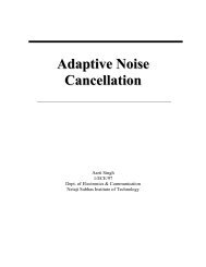
Summary of Search Techniques
Technique Setup Cost Search Cost
Linear search 0, since we’re O(n)
given the list
Binary search O(n log n) O(log n)
to sort the list
Hash table O(n) to fill the
buckets
O(1)
2
1

Trees
3
Trees
• A tree is a hierarchical data structure.
– Every tree has a node called the root.
– Each node can have 1 or more nodes as children.
– A node that has no children is called a leaf.
• A common tree in computing is a binary tree.
– A binary tree consists of nodes that have at most 2
children.
– A complete binary tree has the maximum number of
nodes on each of its levels.
• Applications: data compression, file storage, game
trees
4
2

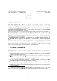
Binary Tree
24
84
41 96
50
98
13
37
Which one is the root?
Which ones are the leaves?
Is this a complete binary tree?
What is the height of this tree?
5
Binary Tree
24
84
41 96
50
98
13
37
The root has the data value 84.
There are 4 leaves in this binary tree: 13, 37, 50, 98.
This binary tree is not complete.
This binary tree has height 3 (depends on the assumed definition. Some
definitions would regard it as 4).
6
3

Binary Trees: Implementation
• One common implementation of binary trees uses
nodes like a linked list does.
– Instead of having a “next” pointer, each node has a
“left” pointer and a “right” pointer.
45
Level 1
31 70
Level 2
19 38 86
Level 3
7
Using Nested Arrays
• Languages like Ruby do not let programmers manipulate pointers
explicitly.
• We could use Ruby arrays to implement binary trees. For example:
[45, left, right]
45
Level 1
31 70
19 38 86
Level 2
Level 3
[45,[31,left,right],[70,left,right]]
[45, [31, [19,[],[]], [38,[],[]]],
[70,[], [86, [], []]]
]
[] stands for an empty tree
Arrows point to subtrees
8
4

Using One Dimensional Arrays
• We could also use a flat array.
45
Level 1
31 70
Level 2
19 38 86
Level 3
45 31 70 19 38 86
Level 1 Level 2 Level 3
9
Dynamic Set Operations
• Insert
• Delete
• Search
• Find min/max
• ...
Choosing a specific data structure has consequences on which
operations can be performed faster.
10
5

Binary Search Tree (BST)
• A binary search tree (BST) is a binary tree
such that
– All nodes to the left of any node have data
values less than that node
– All nodes to the right of any node have data
values greater than that node
11
Inserting into a BST
• For each data value that you wish to insert
into the binary search tree:
– Start at the root and compare the new data
value with the root.
– If it is less, move down left. If it is greater,
move down right.
– Repeat on the child of the root until you end
up in a position that has no node.
– Insert a new node at this empty position.
12
6

Example
• Insert: 84, 41, 96, 24, 37, 50, 13, 98
84
41 96
24
50
98
13
37
15110 Principles of Computing,
Carnegie Mellon University
13
Using a BST
• How would you search for an element in a
BST?
84
41 96
24
50
98
13
37
15110 Principles of Computing,
Carnegie Mellon University
14
7

Searching a BST
• For the key (data value) that you wish to
search
– Start at the root and compare the key with the
root. If equal, key found.
– Otherwise
• If it is less, move down left. If it is greater, move
down right. Repeat search on the child of the root.
• If there is no non‐empty subtree to move to, then
key not found.
15110 Principles of Computing,
Carnegie Mellon University
15
Exercises
• How you would find the minimum and
maximum elements in a BST?
• What would be output if we walked the tree
in left‐node‐right order?
15110 Principles of Computing,
Carnegie Mellon University
16
8

Max‐Heaps
• A max‐heap is a binary tree such that
– The largest data value is in the root
– For every node in the max‐heap, its children
contain smaller data.
– The max‐heap is an almost‐complete binary tree.
• An almost‐complete binary tree is a binary
tree such that every level of the tree has the
maximum number of nodes possible except possibly
the last level, where its nodes are attached as far left
as possible.
15110 Principles of Computing,
Carnegie Mellon University
17
Heap Example
84
41 56
24
10
30
38
13
7
18
9

BSTs vs. Max‐Heaps
• Which tree is designed for easier searching?
• Which tree is designed for retrieving the
maximum value quickly?
• A heap is guaranteed to be “balanced”
(complete or almost‐complete).
What about a BST?
15110 Principles of Computing,
Carnegie Mellon University
19
• BST with n elements
BSTs vs Max‐Heaps
– Insert and Search:
• worst case O(log n) if tree is “balanced”
• worst case O(n) in general since tree could have one
node per level
• Max‐Heap with n elements
– Insert and Remove‐Max
• worst case O(log n) since tree is always “balanced”
– Find‐Max
• worst case O(1) since max is always at the root
15110 Principles of Computing,
Carnegie Mellon University
20
10

Graphs
21
Graphs
• A graph is a data structure that consists of a set of
vertices and a set of edges connecting pairs of the
vertices.
– A graph doesn’t have a root, per se.
– A vertex can be connected to any number of other vertices
using edges.
– An edge may be bidirectional or directed (one‐way).
– An edge may have a weight on it that indicates a cost for
traveling over that edge in the graph.
• Applications: computer networks, transportation
systems, social relationships
22
11

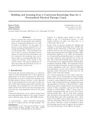
Undirected and Directed Graphs
0
7
0
7
6
1
4
5
3
2
3
6
1
4
2
5
9
3
2
3
from
to
0 1 2 3
0 0 6 7 5
1 6 0 4 ∞
2 7 4 0 3
3 5 ∞ 3 0
from
to
0 1 2 3
0 0 6 7 5
1 ∞ 0 4 ∞
2 2 ∞ 0 3
3 ∞ ∞ 9 0
23
Graphs in Python
from
0
6
4
1
to
7
5
3
0 1 2 3
0 0 6 7 5
2
3
1 6 0 4 ∞
2 7 4 0 3
3 5 ∞ 3 0
graph =
[ [ 0, 6, 7, 5 ],
[ 6, 0, 4, float(‘inf’) ],
[ 7, 4, 0, 3],
[ 5, float(‘inf’), 3, 0] ]
24
12

10
0
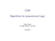
An Undirected Weighted Graph
1
12
6
7
8
3
2
4
5
9
7
4
11
0 1 2 3 4 5 6
Pitt. Erie Will. S.C. Harr. Scr. Phil.
7
6
5
3
from
0 1 2 3 4 5 6
0 0 10 ∞ 8 7 ∞ ∞
1 10 0 12 7 ∞ ∞ ∞
2 ∞ 12 0 6 ∞ 7 5
3 8 7 6 0 9 4 ∞
4 7 ∞ ∞ 9 0 ∞ 11
5 ∞ ∞ 7 4 ∞ 0 3
6 ∞ ∞ 5 ∞ 11 3 0
vertices
edges
to
25
Original Graph
10
Pitt
Erie
8
12
7
6
S.C.
Will.
9
4
5
7
Phil.
Scr.
3
7 Harr.
11
26
13

A Minimal Spanning Tree
Will.
Pitt
Erie
8
7
S.C.
4
5
Phil.
Scr.
3
7
Harr.
The minimum total cost to connect all vertices using edges from
the original graph without using cycles. (minimum total cost = 34)
27
Original Graph
10
Pitt
Erie
8
12
7
6
S.C.
Will.
9
4
5
7
Phil.
Scr.
3
7 Harr.
11
28
14

Shortest Paths from Pittsburgh
10
Pitt
Erie
10
8
7
6
S.C.
Will.
Harr.
4
8
14
7
Phil.
Scr.
3
15
12
The total costs of the shortest path from Pittsburgh to every other
location using only edges from the original graph.
29
Graph Algorithms
• There are algorithms to compute the minimal spanning
tree of a graph and the shortest paths for a graph.
• There are algorithms for other graph operations:
– If a graph represents a set of pipes and the number represent
the maximum flow through each pipe, then we can determine
the maximum amount of water that can flow through the
pipes assuming one vertex is a “source” (water coming into
the system) and one vertex is a “sink” (water leaving the
system)
– Many more graph algorithms... very useful to solve real life
problems.
30
15