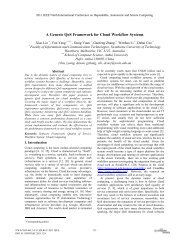
Xiao Liu PhD Thesis.pdf - Faculty of Information and Communication ...

A Novel Probabilistic Temporal
Framework and Its Strategies for Cost-
Effective Delivery of High QoS in
Scientific Cloud Workflow Systems
by
Xiao Liu
B.Mgt. (Hefei University of Technology)
M.Mgt. (Hefei University of Technology)
A thesis submitted to
Faculty of Information and Communication Technologies
Swinburne University of Technology
for the degree of
Doctor of Philosophy
February 2011

To my parents and my wife
I

Declaration
This thesis contains no material which has been accepted for the award
of any other degree or diploma, except where due reference is made in
the text of the thesis. To the best of my knowledge, this thesis contains
no material previously published or written by another person except
where due reference is made in the text of the thesis.
Xiao Liu
February 2011
II

Acknowledgements
I sincerely express my deepest gratitude to my coordinate supervisor, Professor Yun
Yang, for his seasoned supervision and continuous encouragement throughout my
PhD study, especially for his careful reading and appraisal of drafts of this thesis.
Without his consistent support, I would not have been able to complete this
manuscript. To me, he is indeed “a good mentor and a helpful friend”.
I thank Swinburne University of Technology and the Faculty of Information and
Communication Technologies for offering me a full Research Scholarship
throughout my doctoral program. I also thank the Research Committee of the
Faculty of Information and Communication Technologies for research publication
funding support and for providing me with financial support to attend conferences.
My thanks also go to my associate supervisors Dr. Jinjun Chen and Professor
Chengfei Liu, and to staff members, research students and research assistants at
previous CITR/CS3 and current SUCCESS for their help, suggestions, friendship
and encouragement, in particular, Professor Ryszard Kowalczyk, Robert Merkel,
Gillian Foster, Huai Liu, Jianxin Li, Rui Zhou, Jiajie Xu, Minyi Li, Hai Huang,
Xiaohui Zhao, Wei Dong, Jing Gao, Bryce Gibson. Of course, previous and current
members of the Workflow Technology program: Saeed Nauman, Qiang He, Ke Liu,
Dong Yuan, Gaofeng Zhang, Wenhao Li, Dahai Cao and Xuyun Zhang. I also thank
my research partners from Hefei University of Technology (China), Professor
Zhiwei Ni, Yuanchun Jiang, Zhangjun Wu and Qing Lu.
I am deeply grateful to my parents Jianshe Liu and Yousheng Peng for raising me up,
teaching me to be a good person, and supporting me to study abroad. Last but not
least, I thank my wife Nanyan Jiang, for her love, understanding, encouragement,
sacrifice and help.
III

Abstract
Cloud computing is a latest market-oriented computing paradigm which can provide
virtually unlimited scalable high performance computing resources. As a type of
high-level middleware services for cloud computing, cloud workflow systems are a
research frontier for both cloud computing and workflow technologies. Cloud
workflows often underlie many large scale data/computation intensive e-science
applications such as earthquake modelling, weather forecast and Astrophysics. At
build-time modelling stage, these sophisticated processes are modelled or redesigned
as cloud workflow specifications which normally contain the functional
requirements for a large number of workflow activities and their non-functional
requirements such as Quality of Service (QoS) constraints. At runtime execution
stage, cloud workflow instances are executed by employing the supercomputing and
data sharing ability of the underlying cloud computing infrastructures. In this thesis,
we focus on scientific cloud workflow systems.
In the real world, many scientific applications need to be time constrained, i.e.
they are required to be completed by satisfying a set of temporal constraints such as
local temporal constraints (milestones) and global temporal constraints (deadlines).
Meanwhile, task execution time (or activity duration), as one of the basic
measurements for system performance, often needs to be monitored and controlled
by specific system management mechanisms. Therefore, how to ensure satisfactory
temporal correctness (high temporal QoS), i.e. how to guarantee on-time completion
of most, if not all, workflow applications, is a critical issue for enhancing the overall
performance and usability of scientific cloud workflow systems.
At present, workflow temporal verification is a key research area which focuses
on time-constrained large-scale complex workflow applications in distributed high
performance computing environments. However, existing studies mainly emphasise
IV

on monitoring and detection of temporal violations (i.e. violations of temporal
constraints) at workflow runtime, there is still no comprehensive framework which
can support the whole lifecycle of time-constrained workflow applications in order
to achieve high temporal QoS. Meanwhile, cloud computing adopts a marketoriented
resource model, i.e. cloud resources such as computing, storage and
network are charged by their usage. Hence, the cost for supporting temporal QoS
(including both time overheads and monetary cost) should be managed effectively in
scientific cloud workflow systems.
This thesis proposes a novel probabilistic temporal framework and its strategies
for cost-effective delivery of high QoS in scientific cloud workflow systems (or
temporal framework for short in this thesis). By investigating the limitations of
conventional temporal QoS related research, our temporal framework can provide a
systematic and cost-effective support for time-constrained scientific cloud workflow
applications over their whole lifecycles. With a probability based temporal
consistency model, there are three major components in the temporal framework:
Component 1 – temporal constraint setting; Component 2 – temporal consistency
monitoring; Component 3 – temporal violation handling. Based on the investigation
and analysis, we propose some new concepts and develop a set of innovative
strategies and algorithms towards cost-effective delivery of high temporal QoS in
scientific cloud workflow systems. Case study, comparisons, quantitative
evaluations and/or mathematical proofs are presented for the evaluation of each
component. These demonstrate that our new concepts, innovative strategies and
algorithms for the temporal framework can significantly reduce the cost for the
detection and handling of temporal violations while achieving high temporal QoS in
scientific cloud workflow systems.
Specifically, at scientific cloud workflow build time, in Component 1, a
statistical time-series pattern based forecasting strategy is first conducted to predict
accurate duration intervals of scientific cloud workflow activities. Afterwards, based
on the weighted joint normal distribution of workflow activity durations, a
probabilistic setting strategy is applied to assign coarse-grained temporal constraints
through a negotiation process between service users and service providers, and then
fine-grained temporal constraints can be propagated along scientific cloud
workflows in an automatic fashion. At scientific cloud workflow runtime, in
V

Component 2, the state of scientific cloud workflow execution towards specific
temporal constraints, i.e. temporal consistency, is monitored constantly with the
following two steps: first, a minimum probability time redundancy based temporal
checkpoint selection strategy determines the workflow activities where potential
temporal violations take place; second, according to the probability based temporal
consistency model, temporal verification is conducted on the selected checkpoints to
check the current temporal consistency states and the type of temporal violations. In
Component 3, detected temporal violations are handled with the following two steps:
first, an adaptive temporal violation handling point selection strategy decides
whether a temporal checkpoint should be selected as a temporal violation handling
point to trigger temporal violation handling strategies; Second, at temporal violation
handling points, different temporal violation handling strategies are executed
accordingly to tackle different types of temporal violations. In our temporal
framework, we focus on metaheuristics based workflow rescheduling strategies for
handling statistically recoverable temporal violations.
The major contributions of this research are that we have proposed a novel
comprehensive temporal framework which consists of a set of new concepts,
innovative strategies and algorithms for supporting time-constrained scientific
applications over their whole lifecycles in cloud workflow systems. With these, we
can significantly reduce the cost for detection and handling of temporal violations
whilst delivering high temporal QoS in scientific cloud workflow systems. This
would eventually improve the overall performance and usability of cloud workflow
systems because a temporal framework can be viewed as a software service for
cloud workflow systems. Consequently, by deploying the new concepts, innovative
strategies and algorithms, scientific cloud workflow systems would be able to better
support large-scale sophisticated e-science applications in the context of cloud
economy.
VI

The Author’s Publications
Book Chapters:
• X. Liu, D. Yuan, G. Zhang, J. Chen and Y. Yang, SwinDeW-C: A Peer-to-Peer
Based Cloud Workflow System. Handbook of Cloud Computing, pages 309-332,
Springer, ISBN: 978-1-4419-6523-3, 2010.
Journal Papers:
1. X. Liu, Z. Ni, D. Yuan, Y. Jiang, Z. Wu, J. Chen, Y. Yang, A Novel Statistical
Time-Series Pattern based Interval Forecasting Strategy for Activity Durations
in Workflow Systems, Journal of Systems and Software (JSS), Elsevier, vol. 84,
no. 3, pp. 354-376, Mar. 2011.
2. X. Liu, Z. Ni, Z. Wu, D. Yuan, J. Chen and Y. Yang, A Novel General
Framework for Automatic and Cost-Effective Handling of Recoverable
Temporal Violations in Scientific Workflow Systems, Journal of Systems and
Software (JSS), Elsevier, vol. 84, no. 3, pp. 492-509, Mar. 2011.
3. Z. Wu, X. Liu, Z. Ni, D, Yuan and Y. Yang, A Market‐Oriented Hierarchical
Scheduling Strategy in Cloud Workflow Systems, Journal of Supercomputing
(JSC), http://www.ict.swin.edu.au/personal/xliu/papers/JSC-Scheduling.pdf, to
appear (accepted on Sept. 7, 2010), accessed on 1 st Dec. 2010.
4. D. Yuan, Y. Yang, X. Liu and J. Chen, On-demand Minimum Cost
Benchmarking for Intermediate Datasets Storage in Scientific Cloud Workflow
Systems. Journal of Parallel and Distributed Computing (JPDC), in press,
VII

http://dx.doi.org/10.1016/j.jpdc.2010.09.003, 2010.
5. X. Liu, Y. Yang, Y. Jiang and J. Chen, Preventing Temporal Violations in
Scientific Workflows: Where and How, IEEE Transactions on Software
Engineering (TSE), in press, http://doi.ieeecomputersociety.org/10.1109/
TSE.2010.99, (http://www.ict.swin.edu.au/personal/xliu/papers/TSE-2010-01-
0018.pdf), accessed on 1st Nov. 2010.
6. D. Yuan, Y. Yang, X. Liu, G. Zhang and J. Chen, A Data Dependency Based
Strategy for Intermediate Data Storage in Scientific Cloud Workflow Systems,
Concurrency and Computation: Practice and Experience (CCPE), in press,
http://onlinelibrary.wiley.com/doi/10.1002/cpe.1636/pdf, 2010.
7. D. Yuan, Y. Yang, X. Liu and J. Chen, A Data Placement Strategy in Cloud
Scientific Workflows, Future Generation Computer Systems (FGCS), Elsevier,
Vol. 76, No. 6, pp. 464-474, Sept. 2010.
8. X. Liu, Z. Ni, J. Chen and Y. Yang, A Probabilistic Strategy for Temporal
Constraint Management in Scientific Workflow Systems, Concurrency and
Computation: Practice and Experience (CCPE), Wiley,
http://www.ict.swin.edu.au/personal/xliu/doc/ConstraintManagement.pdf, to
appear (accepted on June 17, 2009), accessed on 1 st Nov. 2010.
9. K. Liu, H. Jin, J. Chen, X. Liu, D. Yuan and Y. Yang, A Compromised-Time-
Cost Scheduling Algorithm in SwinDeW-C for Instance-Intensive Cost-
Constrained Workflows on Cloud Computing Platform, International Journal of
High Performance Computing Applications (IJHPC), vol. 24, no. 4, pp. 445-456,
Nov. 2010.
10. Y. Jiang, Y. Liu, X. Liu and S. Yang, Integrating classification capability and
reliability in associative classification: A β-stronger model, Expert Systems with
Applications (ESA), vol. 37, no. 5, pp. 3953-3961, May 2010.
VIII

11. Y. Liu, Y. Jiang, X. Liu and S. L. Yang, CSMC: a combination strategy for
multi-class classification based on multiple association rules, Knowledge-Based
Systems (KBS), vol. 21, no. 8, pp. 786-793, Dec. 2008.
Conference Papers:
12. X. Liu, Z. Ni, Z. Wu, D. Yuan, J. Chen and Y. Yang, An Effective Framework
of Light-Weight Handling for Three-Level Fine-Grained Recoverable Temporal
Violations in Scientific Workflows, Proceedings of the 16 th IEEE International
Conference on Parallel and Distributed Systems (ICPADS10), pp. 43-50,
Shanghai, China, Dec. 2010.
13. Z. Wu, Z. Ni, L. Gu and X. Liu, A Revised Discrete Particle Swarm
Optimisation for Cloud Workflow Scheduling, Proceedings of the 2010
International Conference on Computational Intelligence and Security (CIS2010),
pp. 184-188, Nanning, China, Dec. 2010.
14. X. Liu, J. Chen, Z. Wu, Z. Ni, D. Yuan and Y. Yang, Handling Recoverable
Temporal Violations in Scientific Workflow Systems: A Workflow
Rescheduling Based Strategy, Proceedings of the 10 th IEEE/ACM International
Symposium on Cluster, Cloud and Grid Computing (CCGrid10), pp. 534-537,
May 2010, Melbourne, Victoria, Australia.
15. D. Yuan, Y. Yang, X. Liu and J. Chen, A Cost-Effective Strategy for
Intermediate Data Storage in Scientific Cloud Workflow Systems, Proceedings
of the 24 th IEEE International Parallel & Distributed Processing Symposium
(IPDPS10), Atlanta, USA, Apr. 2010.
16. X. Liu, Y. Yang, J. Chen, Q. Wang and M. Li, Achieving On-Time Delivery: A
Two-Stage Probabilistic Scheduling Strategy for Software Projects, Proceedings
of the 2009 International Conference on Software Process (ICSP09), Lecture
Notes in Computer Science, Vol. 5543, pp. 317-329, Vancouver, Canada, May
2009.
IX

17. X. Liu, J. Chen, and Y. Yang, A Probabilistic Strategy for Setting Temporal
Constraints in Scientific Workflows, Proceedings of the 6 th International
Conference on Business Process Management (BPM2008), Lecture Notes in
Computer Science, Vol. 5240, pp. 180-195, Milan, Italy, Sept. 2008.
18. X. Liu, J. Chen, K. Liu and Y. Yang, Forecasting Duration Intervals of
Scientific Workflow Activities based on Time-Series Patterns, Proceedings of
the 4 th IEEE International Conference on e-Science (e-Science08), pp. 23-30,
Indianapolis, USA, Dec. 2008.
19. Y. Yang, K. Liu, J. Chen, X. Liu, D. Yuan and H. Jin, An Algorithm in
SwinDeW-C for Scheduling Transaction-Intensive Cost-Constrained Cloud
Workflows, Proceedings of the 4 th IEEE International Conference on e-Science
(e-Science08), pp. 374-375, Indianapolis, USA, Dec. 2008.
20. K. Ren, X. Liu, J. Chen, N. Xiao, J. Song, W. Zhang, A QSQL-based Efficient
Planning Algorithm for Fully-automated Service Composition in Dynamic
Service Environments, Proceedings of the 2008 IEEE International Conference
on Services Computing (SCC08), pp. 301-308, Honolulu, Hawaii, USA, July
2008.
X

Table of Contents
CHAPTER 1 INTRODUCTION ............................................................................. 1
1.1 TEMPORAL QOS IN SCIENTIFIC CLOUD WORKFLOW SYSTEMS ..................... 1
1.2 MOTIVATING EXAMPLE AND PROBLEM ANALYSIS ....................................... 3
1.2.1 Motivating Example ................................................................................... 3
1.2.2 Problem Analysis ....................................................................................... 5
1.3 KEY ISSUES OF THIS RESEARCH .................................................................... 7
1.4 OVERVIEW OF THIS THESIS ........................................................................... 9
CHAPTER 2 LITERATURE REVIEW AND PROBLEM ANALYSIS ........... 14
2.1 WORKFLOW TEMPORAL QOS ..................................................................... 14
2.2 TEMPORAL CONSISTENCY MODEL ............................................................. 16
2.3 TEMPORAL CONSTRAINT SETTING ............................................................. 17
2.4 TEMPORAL CHECKPOINT SELECTION AND TEMPORAL VERIFICATION ........ 18
2.5 TEMPORAL VIOLATION HANDLING .............................................................. 20
2.6 SUMMARY .................................................................................................. 21
CHAPTER 3 NOVEL PROBABILISTIC TEMPORAL FRAMEWORK AND
SIMULATION ENVIRONMENTS ...................................................................... 22
3.1 FRAMEWORK OVERVIEW............................................................................ 22
3.2 COMPONENT 1: TEMPORAL CONSTRAINT SETTING .................................... 27
3.3 COMPONENT 2: TEMPORAL CONSISTENCY STATE MONITORING ................ 29
3.4 COMPONENT 3: TEMPORAL VIOLATION HANDLING ..................................... 31
3.5 SIMULATION ENVIRONMENTS .................................................................... 34
3.6 SUMMARY .................................................................................................. 38
COMPONENT I TEMPORAL CONSTRAINT SETTING .............................. 40
CHAPTER 4 FORECASTING SCIENTIFIC CLOUD WORKFLOW
ACTIVITY DURATION INTERVALS ................................................................ 40
4.1 CLOUD WORKFLOW ACTIVITY DURATIONS ............................................... 41
XI

4.2 RELATED WORK AND PROBLEM ANALYSIS ................................................ 43
4.2.1 Related Work......................................................................................... 43
4.2.2 Problem Analysis .................................................................................. 45
4.3 STATISTICAL TIME-SERIES PATTERN BASED FORECASTING STRATEGY ..... 46
4.3.1 Statistical Time-Series Patterns ............................................................. 47
4.3.2 Strategy Overview ................................................................................. 48
4.3.3 Novel Time-Series Segmentation Algorithm: K-MaxSDev ................. 51
4.3.4 Forecasting Algorithms ......................................................................... 54
4.4 EVALUATION .............................................................................................. 58
4.4.1 Example Forecasting Process ................................................................ 58
4.4.2 Comparison Results............................................................................... 62
4.5 SUMMARY .................................................................................................. 66
CHAPTER 5 TEMPORAL CONSTRAINT SETTING ...................................... 68
5.1 RELATED WORK AND PROBLEM ANALYSIS ................................................ 68
5.1.1 Related Work......................................................................................... 68
5.1.2 Problem Analysis .................................................................................. 71
5.2 PROBABILITY BASED TEMPORAL CONSISTENCY MODEL ........................... 72
5.2.1 Weighted Joint Normal Distribution for Workflow Activity Durations72
5.2.2 Probability Based Temporal Consistency Model .................................. 77
5.3 SETTING TEMPORAL CONSTRAINTS ............................................................ 80
5.3.1 Calculating Weighted Joint Distribution ............................................... 81
5.3.2 Setting Coarse-grained Temporal Constraints ...................................... 81
5.3.3 Setting Fine-grained Temporal Constraints .......................................... 83
5.4 CASE STUDY .............................................................................................. 85
5.5 SUMMARY .................................................................................................. 89
COMPONENT II TEMPORAL CONSISTENCY MONITORING ................. 90
CHAPTER 6 TEMPORAL CHECKPOINT SELECTION AND TEMPORAL
VERIFICATION ..................................................................................................... 90
6.1 RELATED WORK AND PROBLEM ANALYSIS ................................................ 91
6.1.1 Related Work......................................................................................... 91
6.1.2 Problem Analysis .................................................................................. 92
6.2 TEMPORAL CHECKPOINT SELECTION AND VERIFICATION STRATEGY ........ 93
6.2.1 Probability Range for Statistically Recoverable Temporal Violations
With Light-Weight Temporal Violation Handling Strategies ........................... 93
6.2.2 Minimum Probability Time Redundancy .............................................. 95
6.2.3 Temporal Checkpoint Selection and Temporal Verification Process ... 97
XII

6.3 EVALUATION .............................................................................................. 98
6.3.1 Experimental Settings ........................................................................... 98
6.3.2 Experimental Results........................................................................... 100
6.4 SUMMARY ................................................................................................ 103
COMPONET III TEMPORAL VIOLATION HANDLING ............................ 104
CHAPTER 7 TEMPORAL VIOLATION HANDLING POINT SELECTION
................................................................................................................................. 104
7.1 RELATED WORK AND PROBLEM ANALYSIS .............................................. 105
7.1.1 Related Work....................................................................................... 105
7.1.2 Problem Analysis ................................................................................ 106
7.2 ADAPTIVE TEMPORAL VIOLATION HANDLING POINT SELECTION STRATEGY
107
7.2.1 Probability of Self-Recovery ............................................................... 107
7.2.2 Temporal Violation Handling Point Selection Strategy ...................... 109
7.3 EVALUATION ............................................................................................ 111
7.4 SUMMARY ................................................................................................ 119
CHAPTER 8 TEMPORAL VIOLATION HANDLING ................................... 120
8.1 RELATED WORK AND PROBLEM ANALYSIS .............................................. 121
8.1.1 Related Work....................................................................................... 121
8.1.2 Problem Analysis ................................................................................ 122
8.2 OVERVIEW OF TEMPORAL VIOLATION HANDLING STRATEGIES ................ 123
8.2.1 Temporal Violation Handling of Statistically Recoverable Temporal
Violations ........................................................................................................ 124
8.2.2 Temporal Violation Handling of Statistically Non-Recoverable
Temporal Violations ........................................................................................ 125
8.3 A GENERAL TWO-STAGE LOCAL WORKFLOW RESCHEDULING STRATEGY
FOR RECOVERABLE TEMPORAL VIOLATIONS ....................................................... 128
8.3.1 Description of The General Strategy ................................................... 128
8.3.2 Metaheuristic Algorithm 1: Genetic Algorithm .................................. 132
8.3.3 Metaheuristic Algorithm 2: Ant Colony Optimisation ....................... 134
8.3.4 Other Representative Metaheuristic Algorithms ................................. 136
8.4 THREE-LEVEL TEMPORAL VIOLATION HANDLING STRATEGY ................. 137
8.5 COMPARISON OF WORKFLOW RESCHEDULING STRATEGIES ..................... 142
8.5.1 Experimental Settings ......................................................................... 142
8.5.2 Experimental Results........................................................................... 145
8.6 EVALUATION OF THREE-LEVEL TEMPORAL VIOLATION HANDLING
XIII

STRATEGY ............................................................................................................ 154
8.6.1 Violation Rates of Local and Global Temporal Constraints ............... 155
8.6.2 Cost Analysis for The Three-Level Handling Strategy ....................... 157
8.7 SUMMARY ................................................................................................ 160
CHAPTER 9 CONCLUSIONS AND FUTURE WORK ................................... 161
9.1 OVERALL COST ANALYSIS FOR THE TEMPORAL FRAMEWORK ................. 161
9.2 SUMMARY OF THIS THESIS ....................................................................... 163
9.3 CONTRIBUTIONS OF THIS THESIS .............................................................. 166
9.4 FUTURE WORK ......................................................................................... 168
BIBLIOGRAPHY ................................................................................................. 171
APPENDIX: NOTATION INDEX ...................................................................... 181
XIV

List of Figures
FIGURE 1.1 EXAMPLE SCIENTIFIC WORKFLOW FOR PULSAR SEARCHING IN
ASTROPHYSICS ..................................................................................................... 4
FIGURE 1.2 THESIS STRUCTURE ................................................................................. 10
FIGURE 3.1 PROBABILISTIC FRAMEWORK FOR TEMPORAL QOS ................................. 23
FIGURE 3.2 SWINCLOUD INFRASTRUCTURE ............................................................... 34
FIGURE 3.3 SWINDEW-C CLOUD WORKFLOW SYSTEM ARCHITECTURE ................... 35
FIGURE 3.4 SWINDEW-C WEB PORTAL ..................................................................... 38
FIGURE 4.1 OVERVIEW OF STATISTICAL TIME-SERIES PATTERN BASED FORECASTING
STRATEGY .......................................................................................................... 49
FIGURE 4.2 BUILDING DURATION SERIES ................................................................... 59
FIGURE 4.3 COMPARISON WITH THREE GENERIC SEGMENTATION ALGORITHMS ....... 60
FIGURE 4.4 PREDICTED DURATION INTERVALS .......................................................... 62
FIGURE 4.5 PERFORMANCE ON TIME-SERIES SEGMENTATION .................................... 62
FIGURE 4.6 ACCURACY OF INTERVAL FORECASTING ................................................. 65
FIGURE 5.1 SEQUENCE BUILDING BLOCK ................................................................... 74
FIGURE 5.2 ITERATION BUILDING BLOCK .................................................................. 75
FIGURE 5.3 PARALLELISM BUILDING BLOCK ............................................................. 76
FIGURE 5.4 CHOICE BUILDING BLOCK ....................................................................... 77
FIGURE 5.5 PROBABILITY BASED TEMPORAL CONSISTENCY MODEL ......................... 79
FIGURE 5.6 NEGOTIATION PROCESS FOR SETTING COARSE-GRAINED TEMPORAL
CONSTRAINTS .................................................................................................... 82
FIGURE 5.7 WEATHER FORECAST SCIENTIFIC CLOUD WORKFLOW SEGMENT ............ 86
FIGURE 6.1 STATISTICALLY RECOVERABLE TEMPORAL VIOLATIONS ........................ 95
FIGURE 6.2 CHECKPOINT SELECTION WITH DIFFERENT NOISES ............................... 102
FIGURE 6.3 CHECKPOINT SELECTION WITH DIFFERENT DISTRIBUTION MODELS ...... 103
FIGURE 7.1 EXPERIMENTAL RESULTS (NOISE=0%).................................................. 115
FIGURE 7.2 EXPERIMENTAL RESULTS (NOISE=5%).................................................. 116
FIGURE 7.3 EXPERIMENTAL RESULTS (NOISE=15%)................................................ 117
XV

FIGURE 7.4 EXPERIMENTAL RESULTS (NOISE=25%)................................................ 118
FIGURE 7.5 COST REDUCTION RATE VS. VIOLATION INCREASE RATE ...................... 119
FIGURE 8.1 TWO-STAGE LOCAL WORKFLOW RESCHEDULING STRATEGY ............... 129
FIGURE 8.2 INTEGRATED TASK-RESOURCE LIST ...................................................... 130
FIGURE 8.3 GA BASED RESCHEDULING ALGORITHM ............................................... 134
FIGURE 8.4 ACO BASED RESCHEDULING ALGORITHM ............................................. 136
FIGURE 8.5 FINE-GRAINED TEMPORAL VIOLATIONS BASED ON THREE TEMPORAL
VIOLATION HANDLING STRATEGIES ................................................................ 137
FIGURE 8.6 PTDA ALGORITHM ................................................................................ 139
FIGURE 8.7 PTDA+ACOWR ALGORITHM ................................................................ 141
FIGURE 8.8 OPTIMISATION ON TOTAL MAKESPAN ................................................... 148
FIGURE 8.9 OPTIMISATION ON TOTAL COST ............................................................. 149
FIGURE 8.10 COMPENSATION ON VIOLATED WORKFLOW SEGMENT ........................ 150
FIGURE 8.11 CPU TIME............................................................................................ 153
FIGURE 8.12 HANDLING OF TEMPORAL VIOLATIONS ............................................... 156
XVI

List of Tables
TABLE 3.1 COMPONENT 1: TEMPORAL CONSTRAINT SETTING ................................... 28
TABLE 3.2 COMPONENT 2: TEMPORAL CONSISTENCY MONITORING .......................... 30
TABLE 3.3 COMPONENT 3: TEMPORAL VIOLATION HANDLING ................................... 32
TABLE 4.1 NOTATIONS USED IN K-MAXSDEV ........................................................... 53
TABLE 4.2 ALGORITHM 1: K-MAXSDEV TIME-SERIES SEGMENTATION .................... 53
TABLE 4.3 ALGORITHM 2: REPRESENTATIVE TIME-SERIES BUILDING ....................... 55
TABLE 4.4 ALGORITHM 3: PATTERN VALIDATION AND TURNING POINTS DISCOVERY
........................................................................................................................... 56
TABLE 4.5 ALGORITHM 4: PATTERN MATCHING AND DURATION INTERVAL
FORECASTING ..................................................................................................... 57
TABLE 4.6 RESULTS FOR SEGMENTATION AND PATTERN VALIDATION ...................... 61
TABLE 4.7 PATTERN DESCRIPTION AND ASSOCIATED TURNING POINTS .................... 61
TABLE 5.1 OVERVIEW ON THE SUPPORT OF TEMPORAL QOS CONSTRAINTS .............. 71
TABLE 5.2 PROBABILISTIC SETTING STRATEGY ......................................................... 80
TABLE 5.3 SPECIFICATION OF THE WORKFLOW SEGMENT ......................................... 87
TABLE 5.4 SETTING RESULTS ..................................................................................... 88
TABLE 7.1 ADAPTIVE TEMPORAL VIOLATION HANDLING POINT SELECTION STRATEGY
......................................................................................................................... 110
TABLE 7.2 EXPERIMENTAL SETTINGS....................................................................... 112
TABLE 8.1 EXPERIMENTAL SETTINGS....................................................................... 143
TABLE 8.2 COMPARISON OF BASIC MEASUREMENTS ............................................... 154
TABLE 8.3 EXPERIMENTAL RESULTS ON THE TIMES OF TEMPORAL VIOLATION
HANDLING ........................................................................................................ 158
XVII

Chapter 1
Introduction
This thesis proposes a novel probabilistic temporal framework to address the
limitations of conventional temporal research and the new challenges for lifecycle
support of time-constrained e-science applications in cloud workflow systems. The
novel research reported in this thesis is concerned with the investigation of how to
deliver high temporal QoS (Quality of Service) from the perspective of cost
effectiveness, especially at workflow runtime. A set of new concepts, innovative
strategies and algorithms are designed and developed to support temporal QoS over
the whole lifecycles of scientific cloud workflow applications. Case study,
comparisons, quantitative evaluations and/or theoretical proofs are conducted for
each component of the temporal framework. This would demonstrate that with our
new concepts, innovative strategies and algorithms, we can significantly improve the
overall temporal QoS in scientific cloud workflow systems.
This chapter introduces the background, motivations and key issues of this
research. It is organised as follows. Section 1.1 gives a brief introduction to temporal
QoS in cloud workflow systems. Section 1.2 presents a motivating example from a
scientific application area. Section 1.3 outlines the key issues of this research.
Finally, Section 1.4 presents an overview for the remainder of this thesis.
1.1 Temporal QoS in Scientific Cloud Workflow Systems
Cloud computing is a latest market-oriented computing paradigm [11, 37]. It refers
to a variety of services available on the Internet that delivers computing
functionality on the service provider’s infrastructure. A cloud is a pool of virtualised
computer resources and may actually be hosted on such as grid or utility computing
environments [7, 59]. It has many potential advantages which include the ability to
1

scale to meet changing user demands quickly; separation of infrastructure
maintenance duties from users; location of infrastructure in areas with lower costs of
real estate and electricity; sharing of peak-load capacity among a large pool of users
and so on. Given the recent popularity of cloud computing, and more importantly
the appealing applicability of cloud computing to the scenario of data and
computation intensive scientific workflow applications, there is an increasing
demand to investigate scientific cloud workflow systems. For example, scientific
cloud workflow systems can support many complex e-science applications such as
climate modelling, earthquake modelling, weather forecast, disaster recovery
simulation, Astrophysics and high energy physics [30, 88, 92]. These scientific
processes can be modelled or redesigned as scientific cloud workflow specifications
(consisting of such as workflow task definitions, process structures and QoS
constraints) at build-time modelling stage [30, 55]. The specifications may contain a
large number of computation and data intensive activities and their non-functional
requirements such as QoS constraints on time and cost [98]. Then, at runtime
execution stage, with the support of cloud workflow execution functionalities such
as workflow scheduling [100], load balancing [12] and temporal verification [19],
cloud workflow instances are executed by employing the supercomputing and data
sharing ability of the underlying cloud computing infrastructures with satisfactory
QoS.
One of the research issues for cloud workflow systems is on how to deliver high
QoS [19, 25]. QoS is of great significance to stakeholders, viz. service users and
providers. On one hand, low QoS may result in dissatisfaction and even investment
loss of service users; on the other hand, low QoS may risk the service providers of
out-of-business since it decreases the loyalty of service users. QoS requirements are
usually specified as quantitative or qualitative QoS constraints in cloud workflow
specifications. Generally speaking, the major workflow QoS constraints include five
dimensions, viz. time, cost, fidelity, reliability and security [98]. Among them, time,
as one of the most general QoS constraints and basic measurements for system
performance, attracts many researchers and practitioners [54, 105]. For example, a
daily weather forecast scientific cloud workflow which deals with the collection and
processing of large volumes of meteorological data has to be finished before the
broadcasting of the weather forecast program every day at, for instance, 6:00pm.
2

Clearly, if the execution time of the above workflow applications exceeds their
temporal constraints, the consequence is usually unacceptable to all stakeholders. To
ensure on-time completion of these workflow applications, sophisticated strategies
need to be designed to support high temporal QoS in scientific cloud workflow
systems.
At present, the main tools for workflow temporal QoS support is temporal
checkpoint selection and temporal verification which deals with the monitoring of
workflow execution against specific temporal constraints and the detection of
temporal violations [20]. However, to deliver high temporal QoS in scientific cloud
workflow systems, a comprehensive temporal framework which can support the
whole lifecycles, viz. from build-time modelling stage to runtime execution stage, of
time-constrained scientific cloud workflow applications needs to be fully
investigated.
1.2 Motivating Example and Problem Analysis
In this section, we present an example in Astrophysics to analyse the problem for
temporal QoS support in scientific cloud workflow systems.
1.2.1 Motivating Example
Parkes Radio Telescope (http://www.parkes.atnf.csiro.au/), one of the most famous
radio telescopes in the world, is serving for institutions around the world. Swinburne
Astrophysics group (http://astronomy.swinburne.edu.au/) has been conducting
pulsar searching surveys (http://astronomy.swin.edu.au/pulsar/) based on the
observation data from Parkes Radio Telescope. The Parkes Multibeam Pulsar
Survey is one of the most successful pulsar surveys to date. The pulsar searching
process is a typical scientific workflow which involves a large number of data and
computation intensive activities. For a single searching process, the average data
volume (not including the raw stream data from the telescope) is over 4 terabytes
and the average execution time is about 23 hours on Swinburne high performance
supercomputing facility (http://astronomy.swinburne.edu.au/supercomputing/).
3

Figure 1.1 Example Scientific Workflow for Pulsar Searching in Astrophysics
For the convenience of discussion, as depicted in Figure 1.1, we only illustrate
the high-level workflow structure and focus on one path in the total of 13 parallel
paths for different beams (the other parallel paths are of similar nature and denoted
by cloud symbols). The average durations (normally with large variances) for highlevel
activities (those with sub-processes underneath) and three temporal constraints
are also presented for illustration. Given the running schedules of Swinburne
supercomputers and the observing schedules for Parkes Radio Telescope
(http://www.parkes.atnf.csiro.au/observing/schedules/), an entire pulsar searching
process, i.e. a workflow instance, should normally be completed in one day, i.e. an
overall temporal constraint of 24 hours, denoted as U (SW ) in Figure 1.1.
Generally speaking, there are three main steps in the pulsar searching workflow.
The first step is data collection (about 1 hour), data extraction and transfer (about 1.5
hours). Data from Parkes Radio Telescope streams at a rate of one gigabit per
second and different beam files are extracted and transferred via gigabit optical fibre.
The second step is data pre-processing. The beam files contain the pulsar signals
which are dispersed by the interstellar medium. De-dispersion is to counteract this
effect. A large number of de-dispersion files are generated according to different
choices of trial dispersions. In this scenario, 1,200 is the minimum number of
dispersion trials, and it normally takes 13 hours to complete. For more dispersion
trials such as 2,400 and 3,600, longer execution time is required or more computing
resources need to be allocated. Furthermore, for binary pulsar searching, every dedispersion
file needs to undergo an Accelerate process. Each de-dispersion file
generates several accelerated de-dispersion files and the whole process takes around
1.5 hours. For instance, if we assume that the path with 1,200 de-dispersion files is
chosen, then a temporal constraint of 15.25 hours, denoted as U ( SW1
) , usually
should be assigned for the data pre-processing step. The third step is pulsar seeking.
Given the generated de-dispersion files, different seeking algorithms can be applied
to search for pulsar candidates, such as FFT Seek, FFA Seek, and single Pulse Seek.
For the instance of 1,200 de-dispersion files, it takes around 1 hour for FFT seeking
4

to seek all the candidates. Furthermore, by comparing the candidates generated from
different beam files in the same time session (around 20 minutes), some interference
may be detected and some candidates may be eliminated (around 10 minutes). With
the final pulsar candidates, the original beam files are retrieved to find their feature
signals and fold them to XML files. The Fold To XML activity usually takes around
4 hours. Here, a temporal constraint of 5.75 hours, denoted as U ( SW2)
, usually
should be assigned. At last, the XML files will be inspected manually (by human
experts) or automatically (by software) to facilitate the decision making on whether
a possible pulsar is found or not (around 20 minutes).
1.2.2 Problem Analysis
Based on the above example, we can see that to guarantee on-time completion of the
entire workflow process, the following problems need to be addressed.
1) Setting temporal constraints. Given the running schedules, global temporal
constraint, i.e. the deadline U (SW ) of 24 hours, needs to be assigned. Based on that,
with the estimated durations of workflow activities, two other coarse-grained
temporal constraints U ( SW1
) and U ( SW2
) are assigned as 15.25 hours and 5.75
hours respectively. These coarse-grained temporal constraints for local workflow
segments can be defined based on the experiences of service providers (e.g. the
estimated activity durations) or the requirements of service users (e.g. QoS
requirements). However, fine-grained temporal constraints for individual workflow
activities, especially those with long durations such as De-dispersion and seeking
algorithms are also required in order to support fine-grained control of workflow
executions. Meanwhile, the relationship between the high-level coarse-grained
temporal constraints and their low-level fine-grained temporal constraints should be
investigated so as to keep the consistency between them.
Therefore, a temporal constraint setting component should be able to facilitate
the setting of both coarse-grained and fine-grained temporal constraints in scientific
cloud workflow systems. Meanwhile, as the prerequisite, an effective forecasting
strategy for scientific cloud workflow activity durations is also required to ensure
the accuracy of the setting results 1 .
2) Monitoring temporal consistency state. Due to the complexity and uncertainty
in the dynamic scientific cloud workflow system environments, the violations of
1
Actually, since estimated activity durations is one of the most important data for the temporal
framework, an effective forecasting strategy is not only required for setting temporal constraints but
also its subsequent components such as checkpoint selection, temporal verification and temporal
violation handling.
5

fine-grained temporal constraints (the overrun of expected individual activity
durations) may often take place. Therefore, temporal consistency states need to be
kept under constant monitoring to detect and handle potential violations in a timely
fashion. For example, during the second step of data pre-processing, delays may
occur in the activity of De-dispersion which needs to process terabytes of data and
consumes more than 13 hours computation time. Here, for example, we assume that
the De-dispersion activity takes 14.5 hours (a delay of 90 minutes, i.e. around 10%
over the mean duration), then given U ( SW1
) of 15.25 hours, there would only be 45
minutes left for the Accelerate activity which normally needs 1.5 hours. Another
example is that during the third step of pulsar seeking, we assume that the overall
duration for the FFT Seek, Get Candidates and Eliminate Candidates activities is
108 minutes (a delay of 18 minutes, i.e. around 20% over the mean duration). In
such a case, given U ( SW2)
being 5.75 hours, there will probably be a 3 minutes
delay if the subsequent activity completes on time. In both examples, time delays
occurred and potential temporal violations may take place.
Therefore, based on the above two examples, we can see that monitoring of
temporal consistency is very important for the detection of temporal violations.
Effective and efficient strategies are required to monitor temporal consistency of
scientific cloud workflow execution and detect potential violations as early as
possible before they become real major overruns.
3) Handling temporal violations. If temporal violations like the two examples
mentioned above are detected, temporal violation handling strategies are normally
required. However, it can be seen that the temporal violations in the two examples
are very different. In the first example with U ( SW1
) , even if we expect the
Accelerate activity can be finished 10 minutes less than its mean duration (around
10% less than the mean duration), i.e. finished in 80 minutes, there would still be a
35 minute time deficit. Therefore, under such a situation, at that stage, some
temporal violation handling strategies should be executed to decrease the duration of
the Accelerate activity to at most 45 minutes by, for instance, rescheduling the Taskto-Resource
assignment or recruiting additional resources in order to maintain
temporal correctness. Cleary, in such a case, a potential temporal violation is
detected where temporal violation handling is necessary. As in the second example
with U ( SW2)
, the 3 minutes time deficit is a small fraction compared with the mean
duration of 4 hours for the Fold to XML activity. Actually, there is a probability that
it can be automatically compensated for since it only requires the Fold to XML
activity to be finished 1.25% shorter than its mean duration. Therefore, in such a
situation, though a temporal violation is detected, temporal violation handling may
6

e unnecessary. Hence, an effective decision making strategy is required to
determine whether a temporal violation handling is necessary or not when a
temporal violation is detected.
If temporal violation handing is determined as necessary, temporal violation
handling strategies will be executed. In scientific cloud workflow systems, every
computing resource may be charged according to its usage. Therefore, besides the
effectiveness (the capability of compensating occurred time deficits), the cost of the
temporal violation handling process should be kept as low as possible. Therefore, on
one hand, different levels of temporal violations should be defined. For example, for
the above mentioned two temporal violations, the first one with larger time deficit
(i.e. 35 minutes) will normally require heavy-weight temporal violation handling
strategies such as recruitment of additional resources; whilst for the second one with
smaller time deficit (i.e. 3 minutes), it could be handled by light-weight strategies or
even by self-recovery (i.e. without any treatment). On the other hand, the capability
and cost for different temporal violation handling strategies should be investigated
so that when specific temporal violations have been detected, the handling strategies
which possess the required capability but with lower cost can be applied accordingly.
Therefore, for the purpose of cost effectiveness, a decision making process on
temporal violation handling is required when a temporal violation is detected.
Meanwhile, a set of cost-effective temporal violation handling strategies are required
to be designed and developed so as to meet the requirements of different levels of
fine-grained temporal violations.
1.3 Key Issues of This Research
This thesis investigates the deficiencies of existing research work on the lifecycle
support of temporal QoS in scientific cloud workflow systems. Firstly, there lacks a
comprehensive temporal framework to support the whole lifecycle of timeconstrained
cloud workflow applications; secondly, the management cost for high
temporal QoS should be proactively controlled by the design of cost-effective
strategies for each component of the framework. With a probability based temporal
consistency model, there are three major components in our temporal framework:
Component 1 – setting temporal constraints; Component 2 – monitoring temporal
consistency; Component 3 – handling temporal violations.
Specifically, at scientific cloud workflow build time, in Component 1, temporal
constraints including both global temporal constraints for entire workflow processes
7

(deadlines) and local temporal constraints for workflow segments and/or individual
activities (milestones) are required to be set as temporal QoS constraints in cloud
workflow specifications. The problem for the conventional QoS constraint setting
strategies lies in three aspects: first, estimated workflow activity durations (based on
user experiences or simple statistics) are often inaccurate in cloud workflow system
environments; second, these constrains are not well balanced between user
requirements and system performance; third, the time overheads of the setting
process is non-trivial, especially for large numbers of local temporal constraints. To
address the above issues, a statistical time-series pattern based forecasting strategy is
first investigated to predict the duration intervals of cloud workflow activities.
Afterwards, based on the weighted joint normal distribution of workflow activity
durations, a probabilistic setting strategy is applied to assign coarse-grained
temporal constraints through a negotiation process between service users and service
providers, and then the fine-grained temporal constraints can be propagated along
scientific cloud workflows in an automatic fashion, i.e. with very small time
overheads.
At scientific cloud workflow runtime, in Component 2, the state of cloud
workflow execution towards specific temporal constraints, i.e. temporal consistency,
is monitored constantly by the checkpoint selection and temporal verification
component. The two major limitations of conventional checkpoint selection and
temporal verification are as follows: first, the selection of multiple types of
checkpoints and the verification of multiple types of temporal consistency states
incur huge cost but most of them are actually unnecessary; second, though the
violations of multiple temporal consistency states can be verified, there is no clear
indication for the level of temporal violations, i.e. it does not support the quantitative
measurement of temporal violations. To address the above issues, with our
probability based temporal consistency model, the probability range for statistically
recoverable and non-recoverable temporal violations are defined in the first place.
Afterwards, we monitor cloud workflow executions through the following two steps:
first, a minimum probability time redundancy based temporal checkpoint selection
strategy determines the activity points where potential temporal violations take place;
second, probability temporal consistency based temporal verification is conducted
on a checkpoint to check the current temporal consistency state and the types of
8

temporal violations, viz. recoverable or non-recoverable.
Finally, in Component 3, detected temporal violations are handled. The
conventional temporal verification philosophy believes that temporal violation
handling should be triggered on every checkpoint, i.e. whenever a temporal violation
is detected. However, the number of checkpoints for large scale scientific workflow
applications is often huge in dynamic cloud computing environments, and thus
results in significant cost on the handling of temporal violations. Therefore, we
design a cost-effective adaptive temporal violation handling point selection strategy
to further decide whether a checkpoint should be selected as a temporal violation
handling point, i.e. temporal violation handling is necessary. Afterwards, when
temporal violation handling points are selected, some temporal violation handling
strategies are triggered to tackle the detected temporal violations. So far, temporal
violation handling strategies in scientific cloud workflow systems have not been
well investigated and the existing strategies are either of low performance or high
cost. Therefore, in our temporal framework, an innovative temporal violation
handling strategy is defined which consists of three levels of temporal violations
(from minor to major) and their corresponding violation handling strategies (from
weak capability to strong capability). In such a case, different levels of temporal
violations can be handled according to the capability of different temporal violation
handling strategies with appropriate costs. Among many others, we focus on costeffective
light-weight metaheuristics based workflow rescheduling strategies for
statistically recoverable temporal violations. Specifically, with the design of a
general two-stage local workflow rescheduling strategy, two representative
metaheuristic algorithms including Genetic Algorithm (GA) and Ant Colony
Optimisation (ACO) are adapted and implemented as candidate temporal violation
handling strategies.
1.4 Overview of this thesis
In particular, this thesis deals with the design of a comprehensive temporal
framework which includes a set of new concepts, strategies and algorithms for the
support of high QoS over the whole lifecycle of scientific cloud workflow
applications. The thesis structure is depicted in Figure 1.2.
9

Figure 1.2 Thesis Structure
10

In Chapter 2, we introduce the related work on temporal QoS in workflow
systems and analyse their limitations. Specifically, a temporal consistency model is
used to define temporal consistency states; temporal constraint setting is to assign
both global and local temporal constraints at workflow build time; temporal
checkpoint selection and temporal verification are the two main steps for monitoring
of workflow execution and detection of temporal violations; temporal violation
handling is to compensate the existing time deficits by temporal violation handling
strategies.
In Chapter 3, the high level description of our probabilistic temporal framework
is presented. The foundation of the temporal framework is a novel probability based
temporal consistency model where fine-grained temporal consistency states can be
quantitatively measured by probability confidence values. In order to facilitate the
lifecycle support of high temporal QoS for scientific cloud workflow applications,
our temporal framework is composed of three main components. The main technical
details of the framework are presented separately in three components, viz.
COMPONENT I for temporal constraint setting, COMPONENT II for temporal
consistency monitoring and COMPONENT III for temporal violation handling. In
addition, for the convenience of thesis presentation, the simulation environment for
evaluation of all the components is also addressed in this chapter.
COMPONENT I consists of two chapters, viz. Chapter 4 and Chapter 5.
In Chapter 4, a statistical time-series pattern based forecasting strategy for
scientific cloud workflow activity duration intervals is described. By investigating
the typical requirements in cloud computing environments, a novel time-series
segmentation algorithm named K-MaxSDev is proposed to discover statistical timeseries
patterns and their associated turning points. After that, accurate duration
intervals can be predicted. Comparison experiments with representative forecasting
strategies are demonstrated to evaluate the effectiveness of our strategy.
In Chapter 5, a probabilistic temporal constraint setting strategy is presented.
Based on the joint weighted normal distribution model, the execution time of a
workflow instance or workflow segments can be estimated effectively and
efficiently with the support of four basic building blocks, viz. sequence building
block, iteration building block, parallelism building block and choice building block.
After that, the coarse-grained temporal constraints are first assigned through a
11

negotiation process between service users and service providers based on either a
time oriented or probability oriented manner. When the coarse-grained temporal
constraints are set, the fine-grained temporal constraints for each individual
workflow activities can be derived and propagated in an automatic fashion.
Therefore, the time overheads and computation cost for temporal constraints setting
are much smaller compared with conventional manual settings. The effectiveness of
the strategy is demonstrated through a case study.
COMPONENT II consists of Chapter 6.
In Chapter 6, the existing state-of-the-art checkpoint selection and temporal
verification strategy is modified to adapt to our probability based temporal
consistency model so that only one type of checkpoint needs to be selected instead
of previous multiple types, and only one type of temporal consistency state needs to
be verified instead of previous multiple types. Accordingly, the minimum
probability time redundancy based checkpoint selection strategy and probability
temporal consistency based temporal verification strategy are provided. The
mathematical proof has demonstrated that our adapted strategy is of the same
necessity and sufficiency as the existing state-of-the-art checkpoint selection
strategy but with better cost-effectiveness.
COMPONENT III consists of Chapter 7 and Chapter 8.
In Chapter 7, an adaptive temporal violation handling point selection strategy is
proposed. Temporal violation handling point selection is a novel idea of our latest
study on workflow temporal verification. Based on the necessary and sufficient
checkpoints, temporal violation handling point selection is to further select a subset
of these checkpoints where the probability of temporal violations is higher than the
specific threshold, i.e. temporal violation handling is indeed necessary. Motivated by
adaptive testing techniques and requirements of cost-effectiveness, our temporal
violation handling point selection strategy can select much fewer violation handling
points than conventional strategies while maintaining satisfactory temporal QoS. In
such a case, the overall cost for handling temporal violations can be significantly
reduced.
In Chapter 8, an overview of temporal violation handling strategies is presented.
Given the basic requirements of automation and cost-effectiveness, we design a
general light-weight two-stage local workflow rescheduling strategy which features
12

a two-stage searching process with metaheuristic algorithms. Such a general
rescheduling strategy can ensure the balance between the execution of workflow
instances with temporal violations and those without temporal violations. With such
a general rescheduling strategy, two metaheuristic algorithms, viz. GA and ACO,
are adapted and implemented, and then their performances are compared in four
different measurements including the optimisation rate of makespan, the
optimisation rate of cost, the time deficit compensation rate and the CPU time.
Afterwards, the three-level temporal violation handling strategy designed in our
temporal framework is presented and followed by comprehensive evaluation on its
performance and cost. As detailed in Section 8.4, the handling strategy consists of
three levels of temporal violations, viz. level I, level II and level III temporal
violations, and their corresponding handling strategies, viz. PTDA (probability time
deficit allocation), ACOWR (ACO based two-stage workflow local rescheduling),
and PTDA+ACOWR (the hybrid of PTDA and ACOWR).
Finally, in Chapter 9, we first make an overall cost analysis for each component
in our temporal framework. Then, we summarise the new ideas discussed in this
thesis, the major contributions of this research, and consequent further research
works.
13

Chapter 2
Literature Review and Problem
Analysis
This chapter reviews the existing work related to temporal QoS. This chapter is
organised as follows. Section 2.1 gives a general introduction of workflow temporal
QoS. Section 2.2 reviews the temporal consistency model. Section 2.3 reviews the
temporal constraint setting. Section 2.4 reviews the temporal checkpoint selection
and temporal verification. Section 2.5 reviews the temporal violation handling. In
each section, the problems with the current work are analysed along the line.
2.1 Workflow Temporal QoS
In a cloud environment, there are a large number of similar or equivalent resources
provided by different service providers. Cloud service users can select suitable
resources and deploy them for cloud workflow applications. These resources may
provide the same functionality, but optimise different QoS measures [81].
Meanwhile, different service users or applications may have different expectations
and requirements. Therefore, it is insufficient for a scientific cloud workflow system
to only consider functional characteristics of workflow applications. QoS
requirements such as time limits (temporal constraints) and budget limits (cost
constraints) for cloud workflow execution also need to be managed by scientific
cloud workflow systems. Service users must be able to specify their QoS
requirements of scientific cloud workflows at build time. Then, the actions taken by
the cloud workflow systems at runtime must be chosen according to the original
14

QoS requirements.
Generally speaking, there are five basic dimensions for cloud workflow QoS, viz.
time, cost, fidelity, reliability and security [98]. Time is a basic measurement of
system performance [1, 2, 49]. For workflow systems, the makespan often refers to
the total time overheads required for completing the execution of a workflow. The
total cost often refers to the monetary cost associated with the execution of
workflows including such as the cost for managing workflow systems and usage
charge of cloud resources for processing workflow activities. Fidelity refers to the
measurement related to the quality of the output of workflow execution. Reliability
is related to the number of failures of workflows. Security refers to confidentiality of
the execution of workflow tasks and trustworthiness of resources. Among them,
time, as a basic measurement of performance and general non-functional
requirement, has attracted most of the attention from researchers and practitioners in
the area of such as Software Engineering [84], Parallel and Distributed Computing
[44, 71] and Service Orientated Architectures [35]. In this thesis, we focus on time,
i.e. we investigate the support of high temporal QoS in scientific cloud workflow
systems.
In the real world, most scientific processes are assigned with specific deadlines
in order to achieve their scientific targets on time. For those processes with
deterministic process structures and fully controlled underlying resources, individual
activity durations, i.e. the completion time of each activity, are predictable and
stable. Therefore, process deadlines can normally be satisfied through a build-time
static scheduling process with resource reservation in advance [36, 100]. However,
stochastic processes such as scientific workflows are characterised with dynamic
changing process structures due to the nature of scientific investigation. Furthermore,
with a vast number of data and computation intensive activities, complex workflow
applications are usually deployed on dynamic high performance computing
infrastructures, e.g. cluster, peer-to-peer, grid and cloud computing [4, 65, 92, 95].
Therefore, how to ensure cloud workflow applications to be finished within specific
deadlines is a challenging issue. In fact, this is why temporal QoS is more
emphasised in large scale distributed workflow applications compared with
traditional centralised workflow applications [1].
In the following sections, we will introduce the current work related to temporal
15

QoS in cloud and conventional workflow systems.
2.2 Temporal Consistency Model
Temporal consistency denotes the consistency between build-time temporal QoS
specifications and runtime workflow execution states, namely temporal correctness.
A temporal consistency model defines different temporal consistency states where a
temporal consistency state measures the execution state of a workflow instance
against specific temporal constraints. It is the fundamental standard for temporal
verification [17]. Intuitively, according to true or false of temporal correctness, the
states of temporal consistency can be defined as either temporal consistency states or
temporal inconsistency states. However, this coarse-grained definition is apparently
too weak for conducting fine-grained analysis and control. Therefore, in recent years,
a multiple-discrete-states based temporal consistency model has been widely
adopted. In order to save huge temporal violation handling cost, besides
conventional temporal consistency state denoted as Strong Consistency (SC),
multiple discrete states differentiate three fine-grained states in the conventional
temporal inconsistency state, i.e. Weak Consistency (WC), Weak Inconsistency (WI)
and Strong Inconsistency (SI) [17]. However, since multiple discrete states are
defined based on the basic static time attributes such as the maximum, minimum and
mean durations of individual workflow activities, complex statistical analysis
models cannot be well supported. Meanwhile, such a model still suffers the
following limitations: first, with qualitative expressions, it is difficult for service
users to understand the level of current temporal violations without sufficient
background knowledge and system information; second, with the definitions of four
coarse-grained temporal consistency states, some unnecessary temporal verification
cost may incur. For example, if the current temporal consistency state is SI, and the
temporal verification may start from SC, then WC and then WI, it will take three
times extra cost to identify the current temporal consistency state.
Given the definition for different temporal consistency states, different levels of
temporal violations can be defined accordingly such as the WC violations (the
violations of WC). However, another critical issue with current temporal consistency
models is that they do not consider the capabilities of specific temporal violation
16

handling strategies employed in a scientific cloud workflow system. In such a case,
it is unclear which temporal violation handling strategy should be applied when a
certain level of temporal violation is detected, and thus will probably result in the
failure of temporal violation handling (for example, when a light-weight temporal
violation handling strategy is applied for a major temporal violation) or the loss of
unnecessary time and budget (for example, when a heavy-weight temporal violation
handling strategy is applied for a minor temporal violation). Therefore, for the
purpose of cost effectiveness, the definition of temporal violations should be able to
facilitate the selection of light-weight temporal violation handling strategies (for
minor temporal violations) and heavy-weight temporal violation handling strategies
(for major temporal violations).
2.3 Temporal Constraint Setting
Temporal constraint setting is to assign temporal constraints in scientific cloud
workflow specifications at build time [16]. Recent studies hold the assumption that
temporal constraints are pre-defined and focus only on runtime monitoring of
temporal consistency states. However, the fact is that efforts put at runtime will be
mostly in vain without build time setting of high quality temporal constraints. The
reason is obvious since the purpose of temporal verification is to identify potential
violations of temporal constraints to minimise the temporal violation handling cost.
Therefore, if temporal constraints are of low quality themselves, temporal violations
may often take place no matter how much efforts have been dedicated by runtime
temporal verification. In the real world, service users normally have limited
knowledge about the performance of the underlying cloud services except their
general descriptions. In such a case, it is difficult for users to estimate the activity
durations or workflow makespan. Therefore, the temporal constraints assigned by
service users are mainly based on their own interests with ignorance of the real
system performance such as system load [54]. Meanwhile, service users usually
prefer to assign only one or several coarse-grained temporal constraints. However,
for the purpose of effectively monitoring a large scale scientific cloud workflow, a
large number of fine-grained temporal constraints are required along cloud
workflow execution. Therefore, scientific cloud workflow systems need to derive
17

fine-grained temporal constraints given the input of coarse-grained temporal
constraints by service users [16, 55].
For cloud workflow systems, the quality of temporal constraints can be
measured by at least two basic criteria: 1) well balanced between user requirements
and system performance; 2) well supported for both overall coarse-grained control
and local fine-grained control. Generally speaking, there are two basic ways to
assign QoS constraints, one is task-level assignment and the other is workflow-level
assignment [98]. Since the whole workflow process is composed of individual tasks,
an overall workflow-level constraint can be obtained by the composition of tasklevel
constraints. On the contrary, task-level constraints can also be assigned by the
decomposition of workflow-level constraints. However, different QoS constraints
have their own characteristics and require in-depth research to handle different
scenarios. Currently, the problem of temporal constraint setting in scientific cloud
workflow systems has not been well investigated.
2.4 Temporal Consistency Monitoring
After temporal constraints are assigned at build time, a cloud workflow instance is
required to be under constant monitoring against temporal violations along the entire
workflow execution at runtime. At present, temporal checkpoint selection and
temporal verification are the two basic steps for runtime monitoring of temporal
consistency states [15]. Temporal checkpoint selection is to select specific activity
points along cloud workflow execution to conduct temporal verification on the fly
[18]. As for temporal verification, it is to check the current temporal consistency
state of cloud workflow execution according to the pre-defined temporal consistency
model [17].
In recent years, many checkpoint selection strategies, from intuitive rule based to
sophisticated model based, have been proposed [34, 64, 105]. The work in [34] takes
every workflow activity as a checkpoint. The work in [64] selects the start activity as
a checkpoint and adds a new checkpoint after each decision activity is executed. It
also mentions a type of static activity point which is defined by users at build-time
stage. Since temporal verification inevitably produces extra cost, a Checkpoint
Selection Strategy (CSS) aims to dynamically select only necessary and sufficient
18

activity points to conduct temporal verification. Here, necessity means that only
those activity points where real temporal inconsistency states take place are selected
and sufficiency means that there are no any omitted activity points [21].
Conventional CSS, e.g. setting checkpoints at the start time and end time of each
activity, selecting each decision activity as checkpoint, usually either chooses
unnecessary checkpoints or misses some of them or both [22]. To address such
issues, a minimum time redundancy based checkpoint selection strategy is proposed
in [21] which only selects an activity point as checkpoint when a temporal violation
is detected. Therefore, it is proved to be of both necessity and sufficiency. As for
temporal verification, its effectiveness and efficiency are highly related to its
corresponding temporal consistency model and CSS [15]. Taking the verification of
weak inconsistency (WI) as an example, with the multiple states based temporal
consistency model and WI minimum time redundancy, only those activity points
where WI violations take place are selected as checkpoints to further verify the
temporal consistency states [17]. Furthermore, for multiple states based temporal
consistency, the relationships between different temporal consistency states such as
WC and WI, WI and SI can be reasoned to further improve the efficiency of
temporal verification. The basic idea is that for a specific temporal constraint, if it is
verified to be a higher consistency states, e.g. SC, then we do not need to check for
WC, WI or SI, and so forth. This rule saves unnecessary cost on temporal
verification [20].
At present, given a specific temporal consistency model, checkpoint selection
and temporal verification are usually investigated together to suit the needs of
different scenarios and improve the overall effectiveness and efficiency in
monitoring runtime temporal consistency. However, due to the dynamic nature of
cloud computing environments, violations of local temporal constraints (local
violations for short) may often take place and result in a large number of
checkpoints. Hence, according to current temporal verification strategy, the
accumulated cost on temporal verification at all the selected checkpoints can be
eventually huge. Therefore, a more cost-effective solution is required to reduce the
whole cost while maintaining the performance of current state-of-the-art checkpoint
selection and temporal verification strategies.
19

2.5 Temporal Violation Handling
After temporal verification, the current temporal consistency state is verified, and if
a temporal violation is identified, the follow-up step is to handle such a violation, i.e.
temporal violation handling. So far, the study on temporal violation handling is still
in its infancy.
Temporal violation handling is very different from conventional violation
handling which mainly deals with functional failures in workflow systems [42, 83].
Usually, after functional failures are detected, violation handling process such as
rollback and recovery is triggered [9]. Another way to prevent functional failures is
to run duplicate instances of the same workflows, and hence if one instance fails, the
others can still be running. However, duplicate instances will result in huge
management cost which is several times higher than the needed execution cost in
general [28]. As for temporal violations, as a type of non-functional QoS failures,
they cannot be handled after they actually took place since no actions in the real
world can reduce the execution time of workflow activities after they have already
been finished. In fact, in a cloud computing environment, if a workflow application
has exceeded its deadline (i.e. the global temporal constraint), the service provider
can do nothing but most likely to pay the penalty according to service contracts or
negotiate with the service user for endurance, i.e. extra waiting time. Therefore,
rather than passive recovery, temporal violations need to be proactively prevented
by temporal verification and temporal violation handling before actual large
overruns take place [56]. In other words, effective handling of local temporal
violations along workflow execution instead of recovery of global temporal
violations is what needs to be investigated for the delivery of high temporal QoS in
scientific cloud workflow systems.
The work in [82] introduces five types of workflow exceptions where temporal
violation can be classified into deadline expiry. Meanwhile, three alternate courses
of recovery action, i.e. no action (NIL), rollback (RBK) and compensate (COM), are
also presented. NIL which counts on the automatic recovery of the system itself is
normally not acceptable for the ‘risk-free’ purpose. As for RBK, unlike handling
conventional system function failures, it normally causes extra delays and makes
current inconsistency state even worse. However, COM, i.e. time deficit
20

compensation, is believed as a suitable recovery action for temporal violation.
One of the representative solutions introduced in [17] is a time deficit allocation
strategy (TDA) which compensates current time deficit by utilising the expected
time redundancies of subsequent activities. However, since time deficit has not been
truly reduced, this strategy can only delay the violations of some local constraints
with no effectiveness on overall constraints, e.g. the deadlines. On the contrary,
workflow rescheduling [101] can indeed make up time deficit by expediting the
execution of those not-yet-commenced workflow activities. However, since general
workflow scheduling is an NP complete problem, extra cost is hence inevitable
[100]. Up to now, there are few efforts dedicated to this topic. However, in order to
deliver high temporal QoS in scientific cloud workflow systems, temporal violation
handling plays a significant role. Therefore, it is important that cost-effective
temporal violation handling strategies should be investigated. As for the
measurement, the key criterion is their performance, i.e. how much time deficit can
be compensated. Meanwhile, the cost of the compensation process (e.g. time
overheads and monetary cost) should also be considered since it is unacceptable if
the cost of the compensation process itself is significant, e.g. exceeding the expected
cost such as the penalty brought by those temporal violations.
2.6 Summary
In this chapter, the literatures and problems for the recent studies related to the
temporal QoS support in scientific cloud workflow systems including temporal
consistency model, temporal constraint setting, temporal consistency monitoring,
and temporal violation handling have been presented. Meanwhile, based on the
literature review and problem analysis, the general requirements for temporal
consistency model, constraint setting, consistency monitoring, and temporal
violations handling have also been discussed.
21

Chapter 3
Novel Probabilistic Temporal
Framework and Simulation
Environment
This thesis proposes a novel comprehensive probabilistic temporal framework to
address the limitations of conventional temporal verification and the new challenges
for cost-effective lifecycle support of time-constrained scientific workflow
applications in cloud workflow systems. This chapter presents a high level
description of our framework and its three major components with technical details
described in the subsequent chapters.
This chapter is organised as follows. Section 3.1 presents the framework
overview. Section 3.2 introduces the design of the first component, i.e. temporal
constraint setting. Section 3.3 introduces the design of the second component, i.e.
temporal consistency monitoring. Section 3.4 introduces the design of the third
component, i.e. temporal violation handing. Section 3.5 introduces our SwinCloud
cloud computing infrastructure and SwinDeW-C cloud workflow prototype which
serve as the simulation environment. Finally, Section 3.6 summarises this chapter.
3.1 Framework Overview
The aim of our novel temporal framework is to provide a cost-effective solution to
deliver high temporal QoS in scientific cloud workflow systems. The temporal
framework is designed to support the whole lifecycle of workflow instances, i.e.
from build time modelling stage to workflow runtime execution stage until
22

successful completion. Specifically, in our temporal framework, the foundation is
the probability based temporal consistency model, and its capability is realised by
three components which supports workflow instances throughout their lifecycles,
including temporal constraints setting, temporal consistency monitoring and
temporal violation handling.
Figure 3.1 The Probabilistic Framework for Temporal QoS
As depicted in Figure 3.1, our probabilistic framework consists of three
components which can provide lifecycle support for high temporal QoS in scientific
cloud workflow systems. The three inner cycles stand for the three important factors
involved in the scientific cloud workflows: real world applications, scientific
workflows, and cloud services. All the basic requirements for scientific cloud
workflows come from real world applications. Real world applications need to be
abstracted by service users with the support of workflow modelling tools and then
create the workflow specifications. With the workflow specifications (usually in the
form of visualised workflow templates) submitted by the service users, scientific
workflows are executed by the cloud workflow systems with the underlying cloud
computing infrastructures. Cloud workflow systems, as a type of platform services
themselves, can utilise many other cloud services which provide software services or
computing services. Evidently, the execution of scientific cloud workflows is
23

complex since scientific workflow instances usually have large-scale sophisticated
processes that contain a large number of data and computation intensive activities.
Meanwhile, the performance of scientific cloud workflow systems is uncertain since
cloud services are generally with highly dynamic performance in the cloud
computing environments. Therefore, due to such process complexity and
performance uncertainty, high temporal QoS cannot be easily achieved without
comprehensively designed framework to support the lifecycle of scientific cloud
workflows. This is the fundamental motivation for our research work presented in
this thesis.
The three components are organised in a cycle which denotes that they are
working in such an order to support the whole lifecycle of scientific cloud
workflows.
The first component is temporal constraint setting which assigns both global
temporal constraints (temporal constraints for entire workflow instances) and local
temporal constraints (temporal constraints for local workflow segments and
individual workflow activities) in scientific cloud workflow specifications at
workflow build time. At this stage, temporal constraints, as a type of QoS
requirements, are to be specified in cloud workflow definitions. With other QoS
constraints such as cost and security, these temporal constraints serve as critical
criteria for the selection of cloud services and the SLA (Service Level Agreement)
management [35]. Afterwards, during cloud workflow runtime, service providers are
obligated to complete workflow processes within those assigned temporal
constraints, otherwise, penalty may be enforced according to the service contracts
signed. Therefore, the setting of high quality temporal constraints is very important
to the successful completion of scientific cloud workflows.
In our temporal framework, the function of temporal constraint setting is realised
through a three-step process. The first step is a forecasting process where the
workflow activity duration intervals are predicted by a time-series forecasting
strategy. The second step is a win-win negotiation process between service users and
service providers to specify the coarse-grained temporal constraints. The third step is
a propagation process where fine-grained temporal constraints are set automatically
based on the results of the second step. The detailed process will be introduced in
Section 3.2 and the algorithms for forecasting and setting will be further presented in
24

Chapter 4 and Chapter 5 respectively.
The second component is temporal consistency monitoring which deals with
monitoring of temporal consistency state against temporal violations. Based on a
temporal consistency model, the temporal consistency states of scientific cloud
workflows should be under constant monitoring in order to detect potential temporal
violations in a timely fashion. However, as mentioned before, the cost of temporal
verification can be very huge due to the complexity and uncertainty in cloud
workflow system environments. Therefore, cost-effective strategies need to be
designed to detect potential temporal violations in an efficient fashion.
In our framework, the function of temporal consistency state monitoring is
realised through a two-step process. The first step is temporal checkpoint selection.
Given the probability based temporal consistency model, our minimum probability
time redundancy based checkpoint selection strategy can choose the minimal set of
activity points (i.e. necessary and sufficient checkpoints) for temporal verification.
The second process is temporal verification which checks the current temporal
consistency states at the selected checkpoints with our probability based temporal
consistency model. In our temporal framework, instead of conventional four types of
checkpoint and temporal consistency states, only one type of checkpoint and
temporal consistency state (i.e. recoverable state) needs to be verified, and thus
reduce the cost of checkpoint selection and temporal verification. The detailed
process will be introduced in Section 3.3 and the algorithms will be further
presented in Chapter 6.
The third component is temporal violation handling which deals with recovery of
temporal violations. Based on the results of the previous component for monitoring
temporal consistency, a necessary and sufficient checkpoint is selected where a
potential temporal violation is detected. Conventional temporal verification work
believes in the philosophy that temporal violation handling should be executed at all
necessary and sufficient checkpoints. However, given the probability of selfrecovery
(i.e. the time deficit can be automatically compensated by the saved
execution time of the subsequent workflow activities), we have identified that such a
philosophy is not necessarily ideal. Therefore, a temporal violation handling point
selection process should be designed to further determine whether temporal
violation handling is necessary at each checkpoint. Here, necessity for temporal
25

violation handling points means that the probability of self-recovery (i.e. the time
deficit can be automatically compensated by the saved execution time of the
subsequent workflow segment) is below a threshold, i.e. the probability of temporal
violations is high enough so that temporal violation handling is necessary. If a
temporal violation handling point is selected, then temporal violation handling
strategies should be executed. In our temporal framework, we mainly focus on those
statistically recoverable temporal violations which can be recovered by light-weight
temporal violation handling strategies 2 . For such a purpose, representative
metaheuristics based workflow rescheduling strategies are investigated, adapted and
implemented under a novel general two-stage local workflow rescheduling strategy
to handle temporal violations. Since our temporal violation handling strategy is fully
automatic and only utilises existing system resources without recruiting additional
ones, the cost of temporal violation handling can be significantly reduced compared
with many conventional heavy-weight temporal violation handling strategies.
In our temporal framework, temporal violation handling is realised through a
two-step process. The first step is an adaptive temporal violation handling point
selection process. Motivated by software testing, a novel adaptive temporal violation
handling point selection strategy is designed which can significantly reduce the
overall cost of temporal violation handling while still maintaining satisfactory
temporal QoS. In our strategy, a temporal violation handling point is selected only
when the probability of self-recovery is below the adaptively adjusted threshold
which denotes the requirement for temporal violation handling. After a temporal
violation handling point is selected, corresponding handling strategies should been
executed. In our framework, a novel temporal violation handling strategy is
implemented which consists of three levels of temporal violations (viz. level I, level,
II and level III temporal violations) and their corresponding handling strategies (viz.
PTDA, ACOWR and PTDA+ACOWR). Our temporal violation handling strategy is
mainly based on ACOWR, an ACO based two-stage local workflow rescheduling
strategy, which attempts to compensate the time deficits with the reduced workflow
execution time through optimising the workflow scheduling plan. Here, “two-stage”
means a two-stage searching process designed in our strategy to strike a balance
2 Statistically recoverable and non-recoverable temporal violations are defined in Section 6.2.1 and
their corresponding light-weight and heavy-weight handling strategies are overviewed in Section 8.2.
26

etween time deficit compensation and the completion time of other activities while
“local” means the rescheduling of “local” workflow segments with “local” resources.
To handle temporal violations, the key optimisation objective for workflow
rescheduling is to maximise the compensation time. However, if we only focus on
the speed-up of the workflow instances which has temporal violations, the
completion time of other activities such as the segments of other workflow instances
and ordinary non-workflow tasks, could be delayed and may violate temporal
constraints of their own, if any. Therefore, a balance between time deficit
compensation and the completion time of other activities needs to be considered.
Otherwise, the overall efficiency of scientific cloud workflow systems will be
significantly deteriorated. As for local rescheduling, it is designed for the
requirement of cost effectiveness. Our temporal violation handling strategy only
utilises existing resources which are currently deployed in the system instead of
recruiting additional resources. Meanwhile, unlike global rescheduling which
modifies the global Task-Resource list for the entire workflow instance, our strategy
only focuses on the local workflow segment and optimises the integrated Task-
Resource list. The detailed process will be introduced in Section 3.4 and the
algorithms will be further presented in Chapter 7 and Chapter 8.
3.2 Component 1: Temporal Constraint Setting
Component 1 is temporal constraint setting. As depicted in Table 3.1, the input
includes process models (cloud workflow process definitions) and system logs for
scientific cloud workflows. The output includes both coarse-grained and finegrained
upper bound temporal constraints. Temporal constraints mainly include
three types, i.e. upper bound, lower bound and fixed-time. An upper bound
constraint between two activities is a relative time value so that the duration between
them must be less than or equal to it. As discussed in [20], conceptually, a lower
bound constraint is symmetric to an upper bound constraint and a fixed-time
constraint can be viewed as a special case of upper bound constraint, hence they can
be treated similarly. Therefore, in this thesis, we focus on upper bound constraints
only.
The first step is to forecast workflow activity duration intervals. Activity
27

duration interval is one of the basic elements for the temporal consistency model.
For workflow activities, the accuracy of their estimated durations is critical for the
effectiveness of our temporal framework. However, forecasting is not a trivial issue
in cloud workflow environments due to its complexity and uncertainty by nature.
For such a purpose, a statistical time-series pattern based forecasting strategy is
designed. Unlike conventional strategies which build forecasting models based on
several dominated affecting factors for activity durations (e.g. CPU load, network
speed and memory space), our forecasting strategy focuses on the performance
patterns of activity durations themselves and try to predict an accurate interval based
on the most similar historical time-series patterns. Details about the forecasting
strategy will be presented in Chapter 4.
Table 3.1 Component 1: Temporal Constraint Setting
The second step is to set coarse-grained temporal constraints. Coarse-grained
temporal constraints are those assigned for entire workflow instances (deadlines)
and local workflow segments (milestones). They are usually specified by service
users based on their own interests. However, as analysed in Section 2.3, to ensure
the quality of temporal constraints, a balance should be considered between the
28

service user’s requirements and the system’s performance. For such a purpose, with
the probability based temporal consistency model, a win-win negotiation process
between service users and service providers is designed to support the setting of
coarse-grained temporal constraints. The negotiation process can be conducted
either in a time-oriented way where the service user suggests new temporal
constraints and the service provider replies with the corresponding probability
consistency state (i.e. probability confidence for completing the workflow instance
within the specified temporal constraint), or in a probability-oriented way where the
service user suggests new probability consistency state and the service provider
replies with the corresponding temporal constraints. Finally, a set of balanced
coarse-grained temporal constraints can be achieved. Details about the setting
strategy for coarse-grained temporal constraints will be presented in Chapter 5.
The third step is to set fine-grained temporal constraints. Given the results of the
previous step, coarse-grained temporal constraints need to be propagated along the
entire workflow instance to assign fine-grained temporal constraints for each
workflow activity. In our strategy, an automatic propagation process is designed to
assign fine-grained temporal constraints based on their aggregated coarse-grained
ones. A case study demonstrates that our setting strategy for fine-grained temporal
constraint is very efficient and accurate. Details about the setting strategy for finegrained
temporal constraints will also be presented in Chapter 5.
3.3 Component 2: Temporal Consistency Monitoring
Component 2 is temporal consistency monitoring. As depicted in Table 3.2, the
input includes temporal constraints assigned by Component 1 at workflow build
time and runtime workflow activity durations for completed activities and predicted
activity duration intervals for those not-yet-commenced activities (based on the
forecasting strategy in Component 1). The output is mainly on the current temporal
consistency state at a selected activity point, i.e. checkpoint. The target of this
component is to keep the cloud workflow execution under constant monitoring and
detect potential temporal violations as early as possible.
29

Table 3.2 Component 2: Temporal Consistency Monitoring
The first step is to select temporal checkpoints. Since it is normally too
expensive to conduct temporal verification at every activity point but insufficient to
conduct temporal verification only at a few pre-defined activity points, the target of
a checkpoint selection strategy (CSS) is to select only necessary and sufficient
activity points where potential temporal violations are detected. Therefore, the cost
of temporal verification will be minimised. In our framework, a minimum
probability time redundancy based checkpoint selection strategy is designed for
selecting only necessary and sufficient checkpoints given our probability based
temporal consistency model. Necessary and sufficient checkpoints serve as
important basis for all the subsequent steps. Details about the checkpoint selection
strategy will be presented in Chapter 6.
The second step is temporal verification. Temporal verification is to verify the
current temporal consistency state so as to determine whether a temporal violation
takes place and/or the level of current temporal violations. Given a specific temporal
consistency model which may define different types of temporal consistency states,
conventional temporal verification may need to be conducted for several times to
identify the current temporal consistency states. For example, in the conventional
multi-states based temporal consistency model, if the current temporal consistency
state is strong inconsistency, then the temporal verification process may be
30

conducted for three times, i.e. starting from the verification of strong consistency,
then weak consistency, then weak inconsistency, before the verification of strong
inconsistency [15]. Therefore, the cost of other three times of temporal verification
is actually unnecessary and should be avoided. In our strategy, with the probability
based temporal consistency model where continuous temporal consistency states are
defined, it is no longer necessary to verify different types of temporal consistency
states as one is sufficient to determine the actual level of temporal violations.
Specifically, each temporal consistency state is associated with a unique probability
value and it is either within the range of statistically recoverable or non-recoverable
temporal violations. Therefore, checkpoint selection and temporal verification are
required to be conducted only once at every activity in our temporal framework.
Details about the temporal verification strategy will be presented in Chapter 6.
3.4 Component 3: Temporal Violation Handling
The third component is temporal violation handling. At a selected temporal violation
handling point, temporal violation handling is to tackle the existing temporal
violations by reducing or ideally removing the occurred time deficits. As depicted in
Table 3.3, the input includes the necessary and sufficient checkpoints, temporal
consistency states and the current workflow scheduling plans (which define the
assignment of workflow activities to computing resources, e.g. virtual machines in
cloud computing environments). The output includes the temporal violation
handling points and regenerated workflow scheduling plans which can reduce or
ideally remove the occurred time deficits of violated workflow instances.
The First step is to select temporal violation handling points. In the conventional
temporal verification work [15, 17, 56], a temporal violation handling point is
regarded the same as a necessary and sufficient checkpoint in nature, i.e. temporal
violation handling should be triggered whenever a temporal violation is detected.
However, due to the dynamic nature of cloud workflow environments, the number
of selected checkpoints can still be very huge especially in large scale scientific
cloud workflow applications. Therefore, given the probability of self-recovery and
motivated by random testing techniques, an adaptive temporal violation handling
point selection strategy is designed to further select a subset of necessary and
31

sufficient checkpoints for temporal violation handling. Those temporal violation
handling points are selected when the probability of self-recovery is below the
adaptively adjusted threshold which represents the necessity for temporal violation
handling. Details about the temporal violation handling point selection strategy will
be presented in Chapter 7.
Table 3.3 Component 3: Temporal Violation Handling
The second step is the execution of temporal violation handling strategy at the
selected handling point. As will be introduced in Section 8.4, in our temporal
framework, three temporal violation handling strategies are employed to tackle three
levels of temporal violations, viz. PTDA (Probability Time Deficit Allocation) for
level I temporal violations, ACOWR (Ant Colony Optimisation based Workflow
Rescheduling) for level II temporal violations, and PTDA+ACOWR (the hybrid
PTDA and ACOWR) for level III temporal violations. Here, in Table 3.3, we take
32

PTDA+ACOWR as an example to introduce the temporal violation handling process.
The details about these strategies will be presented in Chapter 8.
For PTDA+ACOWR, Step 2.1 is to allocate probability time deficit. Based on
PTDA, the occurred time deficit is allocated proportionally to the workflow
activities of the subsequent local workflow segment. The purpose of time deficit
allocation is to ensure the balance among the subsequent workflow activities to
share the time deficit. Unlike the conventional strategy which assigns the time
deficit to all the workflow activities remained in the workflow instance [17], our
strategy only considers the subsequent local workflow segment after the selected
handling point. Therefore, the number of workflow activities involved in the
workflow rescheduling process is significantly reduced and thus can save the
temporal violation handling cost.
Step 2.2 is to generate an integrated Task-VM list. The integrated Task-VM list
represents the current scheduling plan for the activities in the local workflow
segment and their co-allocated tasks. Since the rescheduling of workflow activities
in the local workflow segment will not only change the task assignment of their own
but also inevitably change the task assignment of other co-allocated tasks. Therefore,
if we do not consider the other co-allocated tasks, their execution time will probably
be delayed and may even violate their own temporal constraints, if any. The purpose
for the integrated Task-VM list is to consider all the tasks and virtual machines that
will be affected in the rescheduling process. In such a case, a balance between the
time compensation of violated workflow instance and the overall efficiency of the
cloud workflow system could be achieved. Details about the integrated Task-VM list
will also be presented in Section 8.3.1.
Step 2.3 is to optimise the workflow local scheduling plan. The target of the
optimisation process is to reduce the execution time of the activities in the local
workflow segment so that the occurred time deficit can be compensated. In our twostage
workflow local rescheduling strategy, there are two searching processes. The
first searching process is a metaheuristics based searching process where the overall
makespan and cost for the integrated Task-VM list are being optimised. Here, two
representative metaheuristics including GA and ACO are investigated. As for the
second searching process, selected valid candidates (scheduling plans) are compared
in order to find the best solution where the execution time of the local workflow
33

segment is minimal, i.e. the solution which can compensate the occurred time deficit
as much as possible, or even entirely remove it. Based on such a two-stage searching
process, the balance between the execution of workflow instances with temporal
violations and those workflow instances without temporal violations can be achieved.
3.5 Simulation Environments
The framework proposed in this thesis is being gradually implemented as system
components in our SwinDeW-C (Swinburne Decentralised Workflow for Cloud)
scientific cloud workflow system [53, 59, 96]. SwinDeW-C is a cloud workflow
system prototype built on SwinCloud, a cloud computing test bed. All the simulation
experiments demonstrated in this thesis are conducted in our SwinCloud
environment. Therefore, to present to the readers a clear picture of a scientific cloud
workflow system and avoid the redundancy of the introduction about simulation
environments in the subsequent chapters, SwinDeW-C and SwinCloud are
demonstrated earlier in this section.
The SwinCloud infrastructure and SwinDeW-C architecture are depicted in
Figure 3.2 and Figure 3.3 respectively.
Figure 3.2 SwinCloud Infrastructure
SwinCloud is a cloud computing simulation test bed, on which SwinDeW-C is
34

currently running. It is built on the computing facilities in Swinburne University of
Technology and takes advantage of the existing SwinGrid systems [95]. For
example, the Swinburne Astrophysics Supercomputer Node (http://astronomy.swin.
edu.au/supercomputing/) comprises 145 nodes of Dell Power Edge 1950 nodes each
with: 2 quad-core Clovertown processors at 2.33 GHz (each processor is 64-bit lowvolt
Intel Xeon 5138), 16 GB RAM and 2 x 500 GB drives. We install VMWare [91]
on SwinGrid, so that it can offer unified computing and storage resources. By
utilising the unified resources, we set up data centres that can host applications. In
the data centres, Hadoop [41] is installed that can facilitate MapReduce [38]
computing paradigm and distributed data management.
a a
n
n 1
a a
n3 n 4
an5
an6
aN
a n2
am3
a m 4
am
a m 1
am5
am6
a M
a m2
Figure 3.3 SwinDeW-C Cloud Workflow System Architecture
In general, the type of cloud service can be classified as IaaS (Infrastructure as a
Service), PaaS (Platform as a Service) and SaaS (Software as a Service). Meanwhile,
from the system architecture perspective, the cloud architecture includes four basic
layers from top to bottom: application layer (user applications), platform layer
(middleware cloud services to facilitate the development/deployment of user
35

applications), unified resource layer (abstracted/encapsulated resources by
virtualisation) and fabric layer (physical hardware resources) [11]. Accordingly, the
architecture of SwinDeW-C can also be mapped to the four basic layers. Here, we
present the lifecycle of an abstract workflow application to illustrate the system
architecture. Note that we focus on the system architecture, the introduction on the
cloud management services (e.g. brokering, pricing, accounting, and virtual machine
management) and other functional components are omitted here which can all be
found in [59].
Users can easily gain the access to the SwinDeW-C Web portal via any
electronic devices such as PC, laptop, PDA and mobile phone as long as they are
connected to the Internet. At the workflow build-time stage, given the cloud
workflow modelling tool provided by the Web portal on the application layer,
workflow applications are modelled by users as cloud workflow specifications
(consist of such as task definitions, process structures and QoS constraints). After
workflow specifications are created (static verification tools for such as structure
errors and QoS constraints may also be provided), they can be submitted to any one
of the coordinator peers in the platform layer. Here, an ordinary SwinDeW-C peer is
a cloud service node which has been equipped with specific software services
similar to a SwinDeW-G peer [95]. However, while a SwinDeW-G peer is deployed
on a standalone physical machine with fixed computing units and memory space, a
SwinDeW-C peer is deployed on a virtual machine of which the computing power
can scale dynamically according to task request. As for the SwinDeW-C coordinator
peers, they are super nodes equipped with additional workflow management services
and the knowledge across different clouds compared with ordinary SwinDeW-C
peers.
At the runtime instantiation stage, the cloud workflow specification can be
submitted to any of the SwinDeW-C coordinator peers. Afterwards, the workflow
tasks will be assigned to suitable peers through peer-to-peer (p2p) based
communication between SwinDeW-C peers. Since the peer management such as
peer join, peer leave and peer search, as well as the p2p based workflow execution
mechanism, is the same as in SwinDeW-G system environment. Therefore, the
detailed introduction is omitted here which can be found in [95]. Before workflow
execution, a coordinator peer conducts an assessment on the submitted cloud
36

workflow instance to determine whether it can be accepted or not, given the
specified non-functional QoS requirements under the current pricing model. It is
generally assumed that functional requirements can always be satisfied given the
theoretically unlimited scalability of cloud. In the case where users need to run their
own special programs, they can upload them through the Web portal and these
programs can be automatically deployed in the data centre by the resource manager.
Here, a negotiation process between the user and the cloud workflow service
provider may be conducted if the submitted workflow instance is not acceptable to
the workflow system due to the unacceptable offer on budget or deadline. The final
negotiation result will be either the compromised QoS requirements or a failed
submission of the cloud workflow instance. If all the task instances have been
successfully allocated (i.e. acceptance messages are sent back to the coordinator peer
from all the allocated peers), a cloud workflow instance may be completed with
satisfaction of both functional and non-functional QoS requirements (if without
exceptions). Hence, a cloud workflow instance is successfully instantiated.
Finally, at the runtime execution stage, each task is executed by a SwinDeW-C
peer. In cloud computing, the underlying heterogeneous resources are virtualised as
unified resources (virtual machines). Each peer utilises the computing power
provided by its virtual machine which can easily scale according to the request of
workflow tasks. As can be seen in the unified resource layer of Figure 3.3,
SwinCloud is built on the previous SwinGrid infrastructure at the fabric layer.
Meanwhile, some of the virtual machines can be created with external commercial
IaaS cloud service providers such as Amazon, Google and Microsoft. During cloud
workflow execution, workflow management tasks such as QoS management, data
management and security management are executed by the SwinDeW-C peers.
Users can gain the access to the final results as well as the execution information of
their submitted workflow instances at any time through the SwinDeW-C Web portal.
Based on the design discussed above, we have built a primitive prototype of
SwinDeW-C. The prototype is developed in Java and currently running on the
SwinCloud simulation environment. In the SwinDeW-C prototype, we have
inherited most of SwinDeW-G functions, and further implemented the new
components of SwinDeW-C, so that it can adapt to the cloud computing
environment. Furthermore, we have built a Web portal for SwinDeW-C, by which
37

system users and administrators can access the cloud resources and manage the
applications of SwinDeW-C. The Web portal provides many interfaces to support
both system users and administrators for the following tasks.
Specifically for system users:
browse the existing datasets that reside in different cloud service providers’
data centres;
upload their application data to and download the result data from the cloud
storage;
create and deploy workflows to SwinDeW-C using the modelling tools;
monitor workflow execution.
For system administrators:
coordinate workflow execution by triggering scheduling strategies;
manage application data by triggering data placement strategies;
handle functional and non-functional violations by triggering workflow
exception handling strategies.
Some interfaces of the Web portal are shown in Figure 3.4.
Figure 3.4 SwinDeW-C Web Portal
3.6 Summary
In this chapter, we have presented an overview about our probabilistic temporal
38

framework for cost-effective delivery of high temporal QoS in scientific cloud
workflow systems. With a novel probability based temporal consistency model, our
comprehensive framework includes three components: temporal constraint setting,
temporal consistency monitoring, and temporal violation handling. The steps and
strategies for each component have been described briefly while the details will be
presented in subsequent three parts of this thesis. We have also introduced the
SwinCloud infrastructure and SwinDeW-C cloud workflow prototype which serve
as simulation environments for our temporal framework and all its components.
39

COMPONENT I
Temporal Constraint Setting
Chapter 4
Forecasting Scientific Cloud Workflow
Activity Duration Intervals
As discussed in Chapter 2, workflow activity duration is one of the basic elements in
the temporal consistency model, and thus its accuracy is critical for the effectiveness
of temporal verification and all the other related components such as temporal
checkpoint selection and temporal violation handling. Therefore, an accurate
forecasting strategy is required to predict cloud workflow activity durations.
However, it is not a trivial issue due to the dynamic nature of cloud computing
environments. In this chapter, we present a statistical time-series based forecasting
strategy for scientific cloud workflow activity duration intervals. The comparison
results demonstrate that our strategy has better performance than the other existing
representative strategies.
This chapter is organised as follows. Section 4.1 gives a general introduction
about cloud workflow activity durations. Section 4.2 presents the specifically related
work and problem analysis. Section 4.3 proposes the novel statistical time-series
40

pattern based forecasting strategy. Section 4.4 demonstrates the experimental results.
Finally, Section 4.5 summarises the chapter.
This chapter is mainly based on our work presented in [57, 63].
4.1 Cloud Workflow Activity Durations
Due to the dynamic nature of cloud computing environments, it is a critical yet
challenging issue to maintain high temporal QoS in cloud workflow systems. The
foundation for workflow temporal verification is the temporal consistency model
which consists of three basic elements including temporal constraints, real activity
durations of completed workflow activities and the estimated activity durations of
not-yet-commenced workflow activities. Among them, temporal constraints are
specified at build time and normally remain unchanged at runtime. As for real
activity durations of completed workflow activities, they can be easily obtained at
runtime. However, the estimated activity durations of uncompleted workflow
activities are required both at build time for modelling tasks such as constraint
setting, and at runtime for monitoring tasks such as temporal verification. Therefore,
the accuracy of the estimated activity durations is very important for supporting
temporal QoS in scientific cloud workflow systems.
Interval forecasting for activity durations is to estimate the upper bound and the
lower bound of activity durations. Since the accurate point prediction of activity
duration is very difficult in dynamic system environments, the practical way is to
estimate the activity duration intervals [13]. Moreover, a lot of workflow
management tasks such as load balancing and workflow scheduling need the data on
the upper bound and the lower bound of activity durations in order to make various
decisions. Therefore, effective interval forecasting strategies need to be investigated
for scientific cloud workflow systems. However, it is a non-trivial issue. On one
hand, scientific cloud workflow activity durations consist of complex components.
In workflows, activity duration covers the time interval from the initial submission
to the final completion of a workflow activity. Hence, besides the exact execution
time on allocated resources, they also consist of extra time, i.e. workflow overheads.
According to [72], there exist four main categories of workflow overheads in
scientific applications including middleware overhead, data transfer overhead, loss
41

of parallelism overhead and activity related overhead. Similar overheads also exist
in scientific cloud workflow systems. In scientific cloud workflows, activity
durations involve much more affecting factors than the execution time of
conventional computation tasks which are dominated by the load of high
performance computing resources. On the other hand, the service performance is
highly dynamic. Scientific cloud workflows are deployed on cloud computing
infrastructures where the performance of cloud service is highly dynamic since they
are organised and managed in a heterogeneous and loosely coupled fashion.
Moreover, the workload of these shared resources, such as the computing units, the
storage spaces and the network, keeps changing dynamically. Therefore, many
traditional multivariate models which consist of many affecting factors such as CPU
load, memory space, network speed [31, 93, 103, 104] are either unsatisfactory in
performance or too complex to be applicable in practice, let alone the fact that it is
very difficult, if not impossible, to measure these affecting factors in the distributed
and heterogeneous computing environments such as cloud and grid [33, 40]. There
are also many strategies which define a type of “templates” like models [68, 69].
These models may include workflow activity properties such as workflow structural
properties (like control and data flow dependency, etc.), activity properties (like
problem size, executable, versions, etc.), execution properties (like scheduling
algorithm, external load, number of CPUs, number of jobs in the queue, and free
memory, etc.), and then use “similarity search” to find out the most similar activity
instances and predict activity durations [68]. However, they also suffer the same
problems faced by traditional multivariate models mentioned above.
In this thesis, we focus on data and computation intensive scientific cloud
workflows. In scientific cloud workflows, workflow activities normally occupy
some fixed resources and run continuously for a long time due to their own
computation complexity, for example, the activities for generating large number of
de-dispersion files and the running of seeking algorithms in the pulsar searching
scientific workflow described in Section 1.2.1. The execution time of a
data/computation intensive activity is mainly decided by the average performance of
the workflow system over its lifecycle. Therefore, it is important that the forecasting
strategy in a cloud workflow system can effectively meet such a characteristic.
42

4.2 Related Work and Problem Analysis
4.2.1 Related Work
In this thesis, we focus on time-series based interval forecasting strategies. Five
service performance estimation approaches including simulation, analytical
modelling, historical data, on-line learning and hybrid, are presented in [98]. In
general, time-series forecasting belongs to historical data based approaches.
Currently, much work utilises multivariate models and focuses on the prediction of
CPU load since it is the dominant factor for the durations of computation intensive
activities. Typical linear time-series models such as AR, MA and Box-Jenkins are
fitted to perform host load prediction in [31] where it claims that most time-series
models are sufficient for host load prediction and recommends AR(16) which
consumes miniscule computation cost. The work in [52] proposes a one-step-ahead
and low-overhead time-series forecasting strategy which tracks recent trends by
giving more weight to recent data. A hybrid model which integrates the AR model
with confidence interval is proposed in [97] to perform n-step-ahead load prediction.
A different strategy proposed in [85] predicts application duration with historical
information where search techniques are employed to determine those application
characteristics that yield the best definition of similarity. The work in [3]
investigates extended forecast of both CPU and network load on computation grid to
achieve effective load balancing. The authors in [97] mention the problem of turning
points which causes large prediction errors to time-series models. However, few
solutions have been proposed to investigate more affecting factors and handle
turning points. Different from the above work, there are a few literatures utilise
univariate models. NWS [93] implements three types of univariate time-series
forecasting methods including mean-based, median-based and autoregressive
methods, and it dynamically chooses the one exhibiting the lowest cumulative error
measure at any given moment to generate a forecast. Hence, NWS automatically
identifies the best forecasting methods for any given resource. The work in [33]
proposes a Dynamic Exponential Smoothing (DES) method which forecasts the
future duration only based on its past values. The basic motivation for DES is to
handle the problems of sudden peaks and level switches. DES computes the optimal
43

parameter for different classes of fluctuations and it can consistently outperform the
common prediction methods, such as the NWS predictor, AR(16), and ES [33] in a
grid environment. However, to the best of our knowledge, no existing work has been
proposed so far to effectively address the forecasting of activity durations in
scientific cloud workflow systems.
Time-series patterns are those time-series segments which have high probability
to repeat themselves (similar in the overall shape but maybe with different
amplitudes and/or durations) in a large time-series dataset [13, 39, 45, 57]. Timeseries
patterns can be employed for complex prediction tasks, such as trend analysis
and value estimation in stock market, product sales and weather forecast [43]. The
two major tasks in pattern based time-series forecasting are pattern recognition
which discovers time-series patterns according to the pattern definition, and pattern
matching which searches for the similar patterns with given query sequences. To
facilitate complex time-series analysis such as time-series clustering and fast
similarity search, time-series segmentation is often employed to reduce the variances
in each segment so that they can be described by simple linear or non-linear models
[48]. In general, most segmentation algorithms can be classified into three generic
algorithms with some variations which are Sliding Windows, Top-Down and
Bottom-Up [48]. The process of Sliding Window is like sequential scanning where
the segments keep increasing with each new point until some thresholds are violated.
The basic idea of the Top-Down algorithm is the repetition of the splitting process
where the original time-series is equally divided until all segments meet the stopping
criteria. In contrast to Top-Down, the basic process of the Bottom-Up algorithm is
merging where the finest segments are merged continuously until some thresholds
are violated. The main problem for Sliding Window is that it can only “look
forward” but not “look backward”. The main problem for Top-Down is that it lacks
the ability of merging while the main problem for Bottom-Up is that it lacks the
ability of splitting. Therefore, hybrid algorithms which take advantages of the three
generic algorithms by modifications and combinations are often more preferable in
practice [43, 48, 57, 89].
44

4.2.2 Problem Analysis
In cloud workflow systems, most workflow activities are data and/or computation
intensive which require constant processing of specific resources such as network,
I/O facility, and computing units for a long period of time. For workflow activities
in data/computation intensive scientific applications, two problems of their duration
series are limited sample size and frequent turning points. These two problems are
very common in most scientific applications. Therefore, an effective forecasting
strategy is required to tackle these two problems which are explained as follows.
1) Limited sample size. Current work on the prediction of CPU load such as
AR(16) demands a large sample size to fit the model and at least 16 prior points to
make one prediction. However, this becomes a real issue for scientific workflow
activity duration series. Unlike CPU load which reflects an instant state and the
observations can be measured at any time with high sampling rates such as 1Hz
[103], scientific workflow activity durations denote discrete long-term intervals
since activity instances occur less frequently and take minutes or even hours to be
completed. Meanwhile, due to the heavy workload brought by these activities and
the limits of available underlying resources (given requirements on the capability
and performance), the number of concurrent activity instances is usually constrained
in the systems. Therefore, the duration sample size is often limited and linear timeseries
models cannot be fitted effectively.
2) Frequent turning points. A serious problem which deteriorates the
effectiveness of linear time-series models is the frequent occurrence of turning
points where large deviations from the previous duration sequences take place [103].
This problem resides not only in the prediction of CPU load, but also in the
forecasting of activity durations as observed and discussed in many literature [32,
103]. Actually, due to the large durations and the uneven distribution of activity
instances, the states of the underlying system environment are usually of great
differences even between neighbouring duration-series segments. For example, the
average number of concurrent activity instances in the observation unit of
(10:00am~11:00am) may well be bigger than that of (9:00am~10:00am) due to the
normal schedule of working hours. Therefore, activity instances are unevenly
distributed and frequent turning points are hence often expected. This further
45

emphasises the importance of effective turning points discovery and handling in the
forecasting of scientific workflow activity durations.
In this chapter, to address the above issues, we propose a statistical time-series
pattern based forecasting strategy which can achieve better and maintain consistent
performance in the interval forecasting of activity durations in cloud workflow
systems.
4.3 Statistical Time-Series Pattern Based Forecasting Strategy
In this chapter, we utilise time-series based forecasting models. Time-series models
are probably the most widely used statistical ways for formulating and forecasting
the dynamic behaviour of complex objects [13, 57]. A time series is a set of
observations made sequentially through time. Some representative time series,
including marketing time series, temperature time series and quality control time
series, are effectively applied in various scientific and business domains [45].
Similarly, a cloud workflow activity duration time series, or duration series for short,
is composed of ordered duration samples obtained from cloud workflow system logs
or other forms of historical data. Therefore, duration series is a specific type of time
series in the cloud workflow domain. In this thesis, the term “time series” and
“duration series” can be used interchangeably in most cases. Current forecasting
strategies for computation tasks mainly reside on the prediction of CPU load [3,
103]. However, this is quite different from the prediction of cloud workflow activity
durations due to the reasons mentioned earlier.
In this chapter, instead of applying traditional multivariate models, we conduct
univariate time-series analysis which analyses the behaviour of duration series itself
to build a model for the correlation between its neighbouring samples, or in other
words, forecasting the future activity durations only based on the past activity
durations [13]. Specifically, a novel non-linear time-series segmentation algorithm
named K-MaxSDev is proposed to facilitate a statistical time-series pattern based
forecasting strategy. Two problems of the duration series which seriously hinder the
effectiveness of conventional time-series forecasting strategies are limited sample
size and frequent turning points. Limited sample size impedes the fitting of timeseries
models and frequent turning points where dramatic deviations take place
46

significantly deteriorate the overall accuracy of time-series forecasting. To address
such two problems, we utilise a statistical time-series pattern based forecasting
strategy. First, an effective periodical sampling plan is conducted to build
representative duration series. Second, a pattern recognition process employs our K-
MaxSDev time-series segmentation algorithm to discover the minimum number of
potential patterns which are further validated and associated with specified turning
points. Third, given the latest duration sequences, pattern matching and interval
forecasting are performed to make predictions based on the statistical features of the
best-matched patterns. Meanwhile, concerning the occurrences of turning points,
three types of duration sequences are identified and then handled with different
pattern matching results.
The simulation experiments conducted in our SwinDeW-C cloud workflow
system demonstrate that our time-series segmentation algorithm is capable of
discovering the smallest potential pattern set compared with three generic algorithms,
viz. Sliding Windows, Top-Down and Bottom-Up [48]. The comparison results
further demonstrate that our statistical time-series pattern based strategy behaves
better than several representative time-series forecasting strategies, viz. MEAN [31],
LAST [33], Exponential Smoothing (ES) [33], Moving Average (MA) [13], and
Auto Regression (AR) [13] and Network Weather Service (NWS) [93], in the
prediction of high confidence duration intervals and the handling of turning points.
4.3.1 Statistical Time-Series Patterns
The motivation for pattern based time-series forecasting comes from the observation
that for those duration-series segments where the number of concurrent activity
instances is similar, these activity durations reveal comparable statistical features. It
is obvious that when the number of concurrent activities increases, the average
resources that can be scheduled for each activity decrease while the overall
workflow overheads increase, and vice versa. Similar observation is reported in [32]
between the task execution time and the resource load in a global-scale (grid)
environment. Accordingly, the duration series behaves up and down though it may
not necessarily follow a linear relationship. This phenomenon, for example, is
especially evident when workflow systems adopt market-driven or trust-driven
47

esource management strategies that give preferences to a limited range of resources
[10]. Furthermore, if these segments reappear frequently during a duration series,
they can be deemed as potential patterns which represent unique behaviour of the
duration series under certain circumstances. Therefore, if we are able to define and
discover these typical patterns, the intervals of future durations can be estimated
with the statistical features of the closest patterns by matching the latest duration
sequences. Based on this motivation, here, we present the definition of our statistical
time-series patterns as follows.
Definition 4.1 (Statistical Time-Series Patterns):
For a specific time series T = { X1,
X 2...
X n}
which consists of n observations, its
pattern set is { P 1,
P 2...
P
m
Patterns = m}
where ∑ Length ( P i ) ≤ n . For pattern P i of
i=1
length k , it is a reoccurred segment which has unique statistical features of sample
mean µ and sample standard deviation σ , where µ = ∑ X k and
⎛ k ⎞
σ = ⎜ ∑ ( Xi − µ ) ⎟ ( k −1)
.
⎝i=
1 ⎠
2
Note that in this chapter, since we use statistical features to describe the
behaviour of each time-series segment in an overall sense, the order of patterns is
important for time-series forecasting while the order of sample points within each
pattern is not. Meanwhile, for the purpose of generality, sample mean and standard
deviation are employed as two basic statistical features to formulate each pattern.
However, other criteria such as the median value, the trend and the length of each
segment (the number of samples it consists of), can also be considered to make finegrained
definitions.
k
i=1
i
4.3.2 Strategy Overview
As depicted in the outlier of Figure 4.1, our statistical time-series pattern based
forecasting strategy consists of four major steps which are duration series building,
duration pattern recognition, duration pattern matching and duration interval
forecasting. The inner three circles stand for the three basic factors concerned with
48

activity durations: characteristics of the workflow activities, specifications of
scientific cloud workflows, performance of cloud services.
Figure 4.1 Overview of Statistical Time-Series Pattern based Forecasting
Strategy
Here, we illustrate the process of each step while leaving the detailed algorithms
to Section 4.3.3 to Section 4.3.4.
1) Duration series building. Duration series building is designed to tackle the
problem of limited sample size. Building duration series is actually a sampling
process where the historical durations for a specific activity are sampled at equal
observation unit from cloud workflow system logs or other historical data sources,
and then they are arranged according to the order of their submission time. In our
strategy, we adopt a periodical sampling plan where the samples having their
submission time belonging to the same observation unit of each period are treated as
samples for the same unit. Afterwards, a representative duration series is built with
the sample mean of each unit. This periodical sampling plan effectively solves the
problem of limited sample size and uneven distribution, since samples are assembled
to increase the density of each observation unit. Meanwhile, recurrent frequencies of
duration-series segments are statistically guaranteed. Therefore, we only need to
analyse the representative duration series, and if a pattern is identified for this
representative duration series, it is also statistically a pattern for the whole historical
49

duration series. Note that there are many existing techniques to determine the
specific value of the period [14, 49] and it is strongly dependent on the real world
situation of the cloud workflow system. However, it can also be estimated by system
managers from the main source of system workload. For example, many cloud
workflow systems especially those mainly deal with complex data/computation
intensive scientific processes such as weather forecast and pulsar searching by a
specific group of users, the system work load normally behaves periodically
according to the lifecycle of these workflow processes. Specifically, if these
processes are conducted routinely, say once every day, the system workload
probably also behaves similarly with a period of one day in a rough sense. Therefore,
the value of the period can be first chosen as one day and adjusted according to
historical data.
2) Duration pattern recognition. Duration pattern recognition is to discover
duration-series patterns by an effective pattern recognition process. The pattern
recognition process contains two steps which are time-series segmentation and
pattern validation. The first step is to identify a potential pattern set. For this purpose,
we design a novel non-linear time-series segmentation algorithm named K-MaxSDev
to achieve better performance in the discovery of the potential duration-series
patterns compared with three generic algorithms. These duration-series patterns
reflect the fundamental behaviour patterns of duration series. The second step is to
check the validity of these segments by the minimum length threshold and specify
the turning points for each valid pattern. The minimum length threshold is set to
filter those segments which have no enough samples to make effective pattern
matching. Meanwhile, we emphasise the proactive identification of turning points so
as to eliminate large prediction errors. In our strategy, turning points are defined as
those on the edge of two adjacent segments where the testing criterion is violated.
3) Duration pattern matching. Given the latest duration sequence, duration
pattern matching is to find out the closest pattern with similarity search. The latest
duration sequence is compared with valid duration-series patterns obtained through
pattern recognition. Moreover, due to the occurrences of turning points, three types
of duration sequences including the type where the sequence contains internal
turning points, the type where the next value of the sequence is probably a turning
point and the type for the remainder of the sequences, are first identified and then
50

specified with different means and standard deviations. Here, the distance in
similarity search between two sequences is defined as the absolute differences of
their sample means.
4) Duration interval forecasting. With the pattern matching results (the estimated
mean value and associated turning points), duration intervals are specified
accordingly with a given confidence under the assumption that the samples within a
pattern follow the normal distribution [49].
This section briefly describes the process of our statistical time-series pattern
based forecasting strategy. The technical details will be illustrated in the subsequent
sections.
4.3.3 Novel Time-Series Segmentation Algorithm: K-MaxSDev
In this section, we propose K-MaxSDev, a non-linear time-series segmentation
algorithm which is designed to formulate the duration series with minimal number
of segments, i.e. potential duration-series patterns. Here, K is the initial value for
equal segmentation and MaxSDev is the Maximum Standard Deviation specified as
the testing criterion. The intuition for the initial K equal segmentation is an
efficiency enhancement to the generic Bottom-Up algorithm which normally starts
from the finest equal segments with the length of 2. We modify the initial equal
segments with a moderately larger K which can be either user specified or with the
empirical function proposed later in this section. This modification can save
significant computation time at the initial stage. MaxSDev comes directly from the
requirement for precise interval forecasting where the variances in each segment
need to be controlled within a maximum threshold in order to guarantee an accurate
small bound of the predicted durations, i.e. the duration intervals.
K-MaxSDev is a hybrid algorithm which can be described as follows. It starts
from Bottom-Up with K initial equal-segmentation, followed by the repetitive
process of Sliding Window and Top-Down with the testing criterion of MaxSDev.
Here, the basic merging element of Sliding Window is not a single point but a
segment. Meanwhile, the windows can slide both forward and backward to merge as
many segments as possible. As for Top-Down, it equally splits those segments
which cannot be merged with any neighbours. This repetitive process stops when
51

either the maximum repetition time R is reached or all individual segments cannot
be merged with their neighbours any more. Since the condition of “all individual
segments cannot be merged with their neighbours any more” requires additional
programming (or memory space) to store the segmentation results of the previous
repetition, in practice, setting a maximum repetition time is a more efficient way to
stop the repetition process. Meanwhile, the maximum repetition time can prevent the
occurrence of endless loop (e.g. the deadlock of Split and Merge). According to our
experiments, for most duration series, the repetition process (i.e. the do-until part as
shown in Algorithm 1 in Table 4.2) will be repeated for no more than 3 times in
most cases. Therefore, the maximum repetition time R is set as 5 in this chapter
(including the experiments demonstrated in Section 4.4) but may be changed
according to different system environments. Evidently, the aim here is to discover
the minimum number of segments. The purpose of designing K-MaxSDev rather
than employing existing algorithms is to take full advantage of these three generic
algorithms to achieve a better performance. Specifically, Split is to divide the current
segment into two equal parts. In the case where the current segment has odd number
of sample points, the point at the middle position will be included into the left
2 3 4 5 6 7
segment. For example, if we Split a segment of { p
1 2 , p , p , p , p , p , p } , it then
2 3 4 2 3
becomes { p
1 2 , p , p , p , p , p , p } . Its subsequent sample needs to update their index
2
2
2
1
3
3
3
accordingly. Merge is to merge two neighbouring segments into one. For example, if
1 2 3
2
1 2 3 4 5
we Merge two segments of { p 3 , p , p } and { p , } , it then becomes { p , p , p , p , }.
3
3
1 4 p 4
2
2
2
2
2
2
3 3 3 3 p3
Its subsequent sample needs to update their index accordingly. Delete is to “delete”
the previous segment after Merge, i.e. update the index of the sample points. Like in
the above Merge operation, the fourth segment is deleted, i.e. the previous fifth
segment now becomes the new fourth segment, so does the subsequent segments in
the time series. The notations and the pseudo-code for the K-MaxSDev algorithm are
presented in Table 4.1 and Table 4.2 respectively.
52

Table 4.1 Notations Used in K-MaxSDev
Table 4.2 Algorithm 1: K-MaxSDev Time-Series Segmentation
The empirical function for choosing K is based on the equal segmentation tests.
The candidates of K are defined to be in the form of 2 i and should be a value of no
bigger than n / 4 where i is a natural number and n is the length of the duration
series. Otherwise, K-MaxSDev is turning into Bottom-up with low efficiency. The
process is that we first choose some of the candidates and perform equal
segmentation. We calculate the mean for each segment and rank each candidate
according to the average of the absolute differences between the means of
neighbouring segments. The intuition is that initial segmentation should ensure large
differences between the means of segments, so as to guarantee the efficiency of the
segmentation algorithm. The formula for the empirical function is denoted as
Formula 4.1:
53

k 1
∑ − Mean i + 1 − Mean i
Rank ( k)
= i = 1
k −1
Formula 4.1
The theoretical basis for MaxSDev is Tchebysheff’s theorem [87] which has
been widely used in the statistics theory. According to the theorem, given a number
2
d greater than or equal to 1 and a set of n samples, at least [ 1 ( 1 ) ]
− of the
d
samples will lie within d standard deviations of their mean, no matter what the
actual probability distribution is. For example, 88.89% of the samples will fall into
the interval of ( µ − 3 σ , µ + 3σ
)
. The value of µ and σ can be estimated by the
k
sample mean and sample standard deviation as µ = ∑ Xi
k and
i=1
2
⎛ k ⎞
σ = ⎜ ∑ ( Xi − µ ) ⎟ ( k −1)
respectively. If it happens to be a normal distribution,
i=
1
⎝
⎠
Tchebysheff’s theorem is turning to one of its special cases, i.e. the “3σ ” rule which
means with a probability of 99.73% that the sample is falling into the interval of
( µ 3 σ , µ + 3σ
)
− [49]. Therefore, if we control the deviation to be less than m% of
the mean, then 3σ ≤ m % × µ is ensured. We can thus specify MaxSDev by Formula
4.2:
m% MaxSDev = × µ
Formula 4.2
3
K-MaxSDev is the core algorithm for pattern recognition in our strategy, and it is
applied to discover the minimal set of potential duration-series patterns.
4.3.4 Forecasting Algorithms
As presented in Section 4.3.2, the interval forecasting strategy for workflow
activities in data/computation intensive scientific applications are composed of four
major steps: duration series building, duration pattern recognition, duration pattern
matching, and duration interval forecasting. In this section, we will propose the
detailed algorithms for each step. Note that since pattern matching and interval
forecasting are always performed together, we illustrate them within an integrated
process.
54

1) Duration series building
As mentioned in Section 4.3.2, building the representative duration series is to
address the problem of limited sample size. The representative duration series is
built with a periodical sampling plan where the samples having their submission
time belonging to the same observation unit of each period are treated as samples for
the same unit. Afterwards, a representative duration series is built with the sample
mean of each unit. The pseudo-code for the algorithm is presented in Table 4.3
(Algorithm 2). Here, the specific value of the period can be either user defined or
obtained by existing techniques.
Table 4.3 Algorithm 2: Representative Time-Series Building
2) Duration pattern recognition
The duration pattern recognition process consists of two steps which are timeseries
segmentation and pattern validation. The time-series segmentation step is to
discover the minimal set of potential patterns with our novel K-MaxSDev non-linear
time-series segmentation algorithm as proposed in Section 4.3.3. Therefore, its
pseudo-code is omitted here. The pseudo-code for the second step of pattern
validation together with turning points discovery is presented in Table 4.4
(Algorithm 3). With the segmented duration series, namely the discovered potential
duration-series patterns, we further check their validity with the specified minimum
length threshold defined as Min_pattern_length which should be normally larger
than 3 in order to get effective statistics for pattern matching and interval forecasting.
Afterwards, we identify those turning points associated with each valid pattern.
Specifically, turning points are defined as the points where the testing criterion of
55

MaxSDev is violated. Since our K-MaxSDev segmentation algorithm actually
ensures that the violations of MaxSDev only occur on the edge of two adjacent
segments, as shown in Table 4.4, turning points are either specified by the mean of
the next invalid pattern or the first value of the next valid pattern. Evidently, this
specification of turning points captures the locations where large prediction errors
mostly tend to happen.
Table 4.4 Algorithm 3: Pattern Validation and Turning Points Discovery
3) Pattern matching and interval forecasting
The most important issue for pattern matching and interval forecasting is to
identify the type of the given latest duration sequence. Specifically, three types of
duration sequences are defined in this chapter including the type where the sequence
contains internal turning points, the type where the next value of the sequence is
probably a turning point and the type for the remainder of the sequences. As
presented in Table 4.5 (Algorithm 4), the types of sequences are identified based on
standard deviations.
56

Table 4.5 Algorithm 4: Pattern Matching and Duration Interval Forecasting
For the first type of duration sequence which has a standard deviation larger than
MaxSDev, it cannot be matched with any valid patterns and must contain at least one
turning point. Therefore, we need to first locate the turning points and then conduct
pattern matching with the remainder of the duration sequence. However, to ensure
the effectiveness of the prediction, if the length of the remaining duration sequence
is smaller than the minimum pattern length, the duration interval is specified with
the mean of the duration sequence while its standard deviation is substituted by
MaxSDev. Note that the matched pattern is defined as the valid pattern of which the
statistical mean has the minimum absolute difference with that of the latest duration
sequence. As for the second type, it is identified when the standard deviation of the
latest duration sequence is larger than that of the matched pattern but smaller than
MaxSDev. In this case, the next value of the sequence will probably be a turning
point since it is on the edge of two different patterns according to our pattern
recognition process. Therefore, the mean of the next value is specified with the
associated turning point of its matched pattern and the standard deviation is
specified with MaxSDev. For the third type of sequence where its standard deviation
is smaller than its matched pattern, the next value is predicted with the statistical
features of the matched patterns as a refinement to that of the latest duration
57

sequence. As presented in Table 4.5, we illustrate the specification of duration
intervals with normal distribution which is a kind of symmetric probability
distribution. For example, given λ which is the α%
normal distribution, the predicted %
confidence percentile for
α confidence interval is ( µ λσ µ + λσ )
− , ,
where µ and σ stands for the statistical sample mean and standard deviation
respectively. In our strategy, µ and σ are specified according to different types of
duration sequences. However, if the duration samples of a pattern follow nonnormal
distribution models, such as uniform and exponential, changes can be made
to the predicted intervals accordingly [87].
4.4 Evaluation
In this section, we demonstrate the results of a large scale comprehensive simulation
experiments to verify the performance of our time-series pattern based interval
forecasting strategy over the other representative strategies in the cloud workflow
system SwinDeW-C. The simulation data and related materials can be found online 3 .
4.4.1 Example Forecasting Process
In this section, an example is first presented to illustrate the whole forecasting
process in detail. Afterwards, the results of a large scale comparison experiment are
demonstrated. Specifically, on the performance of time-series segmentation, the
three generic time-series segmentation algorithms, Sliding Window, Top-Down and
Bottom-Up, are compared with our novel hybrid algorithm K-MaxSDev. On the
performance of interval forecasting, 6 representative time-series forecasting
strategies widely used in traditional workflow systems including LAST, MEAN,
Exponential Smoothing (ES), Moving Average (MA), Autoregression (AR) and
Network Weather Service (NWS) are compared with our statistical time-series
pattern based interval forecasting strategy based on the same samples.
Here, we illustrate an example forecasting process. To ensure the
representativeness, a selection process is first conducted in workflow specifications
3 http://www.ict.swin.edu.au/personal/xliu/doc/IntervalForecasting.rar.
58

to search for those activities which are both computation and data intensive, and also
with moderate mean durations according to the statistics of the system logs. Here,
we randomly choose one of them to demonstrate the detailed forecasting process.
Now, we demonstrate the simulation experiment with each step addressed in Section
4.3.4.
(a) 15 historical Duration Series
(b) The Representative Duration Series
Figure 4.2 Building Duration Series
1) Duration series building. The first step is to build the duration series. Here, we
set the basic observation time unit as 15 minutes and the overall observation window
as a typical working day of (8:00am~8:00pm). As depicted in Figure 4.2(a), with the
period of a day, 15 duration series are built by random sampling without
replacement in each observation unit. Here, null values are replaced by the unit
sample means plus white noise [49], i.e. a random number with the mean of 0 and
standard deviation of 1. Eventually, the representative duration series is built by the
composition of the sample mean in each observation unit sequentially through the
59

time. As depicted in Figure 4.2(b), the representative duration series which is to be
further analysed lies between the upper and the lower duration series which are
composed of the maximum duration and minimum duration of each observation unit
respectively. In Figure 4.2, the vertical axis stands for the activity durations with the
basic time unit of second.
2) Duration pattern recognition. In this step, we first conduct the K-MaxSDev
time-series segmentation algorithm to discover the potential pattern set. Here, we
need to assign the value for two parameters: K and MaxSDev. Based on our
empirical function, we choose the candidates of 2, 4, 8, and 12. With Formula 4.1 in
Section 4.3.3, 4 is ranked the best. As for MaxSDev, based on Formula 4.2 in
Section 4.3.3 with the overall sample mean µ as 44.11 and having the candidates of
m as 15, 20, 25, and 30, they are specified as 2.21, 2.94, 3.68 and 4.41 respectively.
We conduct K-MaxSDev and compare with the three generic segmentation
algorithms. With different MaxSDev, the number of segments for the four rounds of
test is presented in Figure 4.3. Evidently, with 11, 8, 7 and 5 as the minimum
number of segments in each round of test, K-MaxSDev achieves the best
performance in terms of discovering the smallest potential pattern set.
Nubmer of Segments
20
16
12
8
4
0
MaxSDev:2.21 2.94 3.68 4.41
Sliding
Window
Top-Down
Bottom-up
K-MaxSDev
Figure 4.3 Comparison with Three Generic Segmentation Algorithms
Moreover, with MaxSDev as 2.21 and Min_pattern_length as 3 which is the
lowest bound, the result for segmentation and pattern validation is presented as an
example in Table 4.6 where 8 valid patterns are identified from a total of 11
segments. The valid patterns and their associated turning points are listed in Table
4.7. Note that since our observation period is a whole working day, the turning point
of Pattern 8 is actually defined as the first value of Pattern 1 to make it complete as a
60

cycle. Here, we also trace back the number of concurrent activities according to the
observation units covered by each pattern. The result shows that when the average
number of concurrent activities increases with the schedule of working hours, the
sample means of activity durations also follow an increasing trend. However, they
are evidently not in a linear relationship. Therefore, this observation indeed supports
our motivation.
Table 4.6 Results for Segmentation and Pattern Validation
Table 4.7 Pattern Description and Associated Turning Points
3) Duration pattern matching and 4) Duration interval forecasting. Since these
two steps are highly correlated, we demonstrate them together. Here, we randomly
select 30 duration sequences from the system logs where the lengths range from 4 to
6 and the last value of each sequence is chosen as the target to be predicted. In our
experiment, we adopt the normal distribution model to specify the duration intervals
with a high confidence of 95% [87]. As shown in Figure 4.4, for 25 cases, the target
value lies within the predicted duration intervals. As for the rest of the 5 cases, the
target values deviate only slightly from the intervals. Therefore, the performance of
interval forecasting is effective.
61

Activity Durations
70
60
50
40
30
20
10
0
1 2 3 4 5 6 7 8 9 10 11 12 13 14 15 16 17 18 19 20 21 22 23 24 25 26 27 28 29 30
Figure 4.4 Predicted Duration Intervals
Lower
Limit
Actual
Value
Upper
Limit
Sequence
No
4.4.2 Comparison Results
Here, we first demonstrate the comparison results on the performance of time-series
segmentation. Similar to the example presented above, a total of 100 test cases of
time series, each stands for an independent activity, are randomly selected and tested
with segmentation algorithm. As discussed in Section 4.3.3, given the same testing
criterion, i.e. with the maximum standard deviation, the smaller the number of
segments, the better the segmentation performance is.
Figure 4.5 Performance on Time-Series Segmentation
As can be seen in Figure 4.5, in most cases, our novel hybrid time-series
segmentation algorithm K-MaxSDev behaves the best and achieves the minimal
number of segments which build up the effective basis for time-series pattern
62

ecognition. Sliding Window ranks in the second place, but since it lacks the ability
of looking backwards, it tends to over segment when the system performance is
stable (i.e. the number of segments is small) such as the test cases of 11, 33, 48 and
53. Bottom-Up ranks the third place but since it lacks the ability of splitting, it tends
to over segment when the system performance is dynamic such as the test cases of
12, 20, 47 and 76. When the system performance is less dynamic (e.g. the number of
segments is around 4 to 5 as depicted in Figure 4.5, its performance is close to that
of Sliding Window. Top-Down behaves the worst in most cases due to its nature for
over-segmenting. Since the only action for Top-Down is splitting and it stops the
segmentation process as long as the testing criterion is met, Top-Down ignores the
probability of merging small segments into large ones. Therefore, Top-Down
usually has more segments than others.
Before we demonstrate the comparison results on the accuracy of interval
forecasting, we briefly review the 6 representative forecasting strategies and
introduce the setting of their parameters. Here, the actual value of the k th point is
denoted as Y k and the predicted value for the k th point is denoted as P k . The length
of the latest duration sequence is randomly selected from 4 to 8.
1) LAST. LAST takes the last value of the time series as the predicted value for
the next point. Therefore, Formula 4.3 for LAST is defined as follows:
P k = Y k −1 ( ≥ 1
k ) Formula 4.3
In the experiments, LAST takes the last point of the latest duration sequence as
the predicted value.
2) MEAN. MEAN takes the mean value of all its previous points as the predicted
value for the next point. Therefore, Formula 4.4 for LAST is defined as follows:
1 k −1
i=
0
P k = ∑Y i ( k ≥ 1) Formula 4.4
k
In the experiments, MEAN takes the mean value of the entire time series where
the latest duration sequence belongs to.
3) Exponential Smoothing (ES). ES makes the prediction for the next value
based on both the actual value and the predicted value of its previous point. ES does
not react directly to peaks while it reacts fast enough to significant changes of the
mean values (e.g. the changes from one segment to another segment). The parameter
63

α depends on the characteristics of the dataset. The Formula 4.5 for ES is defined
as follows:
P α ( 0 < α < 1) Formula 4.5
k = Yk
−1 + ( 1−
) Pk
−1
In the experiments, ES applies to the latest duration sequence with α as 0.5 (a
common choice given no priori knowledge).
4) Moving Average (MA). The generic MA predicts the next value based on the
average value of the latest K points, denoted as MA(K). There are also many other
modified versions of MA such as the Weighted MA and Exponential MA [33].
Formula 4.6 for the generic MA(K) is defined as follows:
1 i+
k −1
P i+
k = ∑Yi
( i ≥ 0 , k ≥ 1) Formula 4.6
k
j=
i
In the experiments, MA applies to the latest duration sequence and K is set
randomly from 4 to 8, i.e. the average length of the duration sequences.
5) Autoregression (AR). AR multiplies previous data points with some
parameters between 0 and 1 to predict the next value. These parameters can be
deemed as weights assigned for each point where normally the closer the time, the
larger the weight is. Formula 4.7 for the generic AR(K) is defined as follows:
α
α
Pi
+ k = iYi
+ i+
1 Yi
+ 1 + ... + i+
k −1Y
i+
k −1
j = i+
k −1
( ∑ α j = 1)
j = i
α
Formula 4.7
In the experiments, the value of α i is defined according to Formula 4.8:
⎧ K
⎪ 1−
∑αi
, i = 1
α i
i = = 2
⎨
Formula 4.8
⎪
1 , 2 ≤ Dis ≤ K
⎪ 2
⎩ Dis × 0.9
Here, the distance of the points, denoted as Dis , is defined based on the
positions, i.e. for the last point in the latest duration sequence, its Dis is defined as 1,
and for the second last, its Dis is defined as 2, and so on and so forth. Obviously, as
defined in Formula 4.8, the weight of each point decreases as its distance increases.
6) Network Weather Service (NWS). NWS conducts postcasters using different
windows of previous data and records the “winning” forecaster for each window
size, i.e. the one with the minimal prediction errors on the last point afterwards, the
64

predicted value will be the one predicted by the winning forecaster. The common
forecasters included are Mean/Median, Moving Average/Median, LAST and ES.
Therefore, the formula for the NWS can be described using Formula 4.9:
{ forecaster Min( Err(
P forecaster ))}
Pk
= Pk
| i
k−1 i
( k ≥ 1)
Formula 4.9
In the experiments, the forecasters included in NWS are all the other 5
forecasting strategies listed here. Therefore, based on the current performance, NWS
dynamically selects the best forecasting strategies among LAST, MEAN, ES, MA,
and AR.
The comparison results on the accuracy of interval forecasting are presented in
Figure 4.6. Here, accuracy means that the actual value is within the predicted
interval.
A total of 100 test cases, namely duration sequences, are randomly selected from
those duration-series with the mean durations around 20 to 40 minutes, and applied
with each forecasting strategy. Since despite our K-MaxSDev, all the other
forecasting algorithms are all dedicated to point forecasting, in the experiments, their
upper bounds and lower bounds are defined as the predicted value plus 10% of itself
and the predicted value minus 10% of itself respectively. Therefore, an interval with
the length of 20% of the predicted value is created.
Figure 4.6 Accuracy of Interval Forecasting
As can be seen in Figure 4.6, our pattern based forecasting strategy (denoted as
65

K-MaxSDev) gains a large improvement on the average accuracy of interval
forecasting over the other representative forecasting strategies. The average
accuracy of our K-MaxSDev is 80% while that of the other strategies are mainly
around 40% to 50%. Among the other 6 strategies, AR behaves the best while the
others have similar performance except MEAN which behaves poorly compared
with the others. However, such results actually demonstrate the highly dynamic
performance of the underlying services in cloud workflow systems.
To conclude, in comparison to other representative forecasting strategies in
traditional workflow systems, our forecasting strategy can effectively address the
problems of limited sample size and frequent turning points, and hence achieve
higher accuracy.
4.5 Summary
Interval forecasting for activity durations in cloud workflow systems is of great
importance since it is related to most of cloud workflow QoS and non-QoS
functionalities such as load balancing, workflow scheduling and temporal
verification. However, predicting accurate duration intervals is very challenging due
to the dynamic nature of cloud computing infrastructures. Most of the current work
focuses on the prediction of CPU load to facilitate the forecasting of computation
intensive activities. In fact, the durations of scientific cloud workflow activities are
normally dominated by the average performance of the workflow system over their
lifecycles. Therefore, the forecasting strategies in cloud workflow systems should be
able to adapt to the characteristics of scientific cloud workflow activities.
In this chapter, rather than fitting conventional linear time-series models which
are not ideal, we have investigated the idea of pattern based time-series forecasting.
Specifically, based on a novel non-linear time-series segmentation algorithm named
K-MaxSDev, a statistical time-series pattern based forecasting strategy which
consists of four major functional components: duration series building, duration
pattern recognition, duration pattern matching, and duration interval forecasting,
have been proposed. K-MaxSDev includes an offline time-series pattern discovery
process and an online forecasting process. The simulation experiments conducted in
our SwinDeW-C cloud workflow system have demonstrated that our time-series
66

segmentation algorithm is capable of discovering the smallest potential pattern set
compared with three generic algorithms: Sliding Windows, Top-Down and Bottom-
Up. The large scale comparison results have further demonstrated that our statistical
time-series pattern based strategy behaves better than other 6 representative timeseries
forecasting strategies including LAST, MEAN, Exponential Smoothing,
Moving Average, Autoregression and Network Weather Service in the prediction of
high confidence duration intervals and the handling of turning points. Based on the
accurate forecasting results of our strategy, the efficiency and effectiveness of the
subsequent steps in the temporal framework can be significantly enhanced.
Therefore, overall cost for supporting high temporal QoS can be reduced.
In the future, we will investigate the adaptation of our forecasting strategy for
the mixed types of time-series patterns which may follow both normal and nonnormal
probability distribution models. In such a case, the forecasting accuracy
could be further improved.
67

Chapter 5
Temporal Constraint Setting
As one of the most important workflow QoS dimensions and the focus in this thesis,
the temporal constraint is the foundation of the entire temporal framework.
Temporal constraint setting is to deal with temporal QoS specifications at workflow
build time. As mentioned earlier, high temporal QoS cannot be achieved without
proper setting of high quality temporal constraints.
This chapter presents a probabilistic strategy for setting temporal constraints.
Section 5.1 introduces the specifically related work and problem analysis. Section
5.2 presents probability based temporal consistency model. Section 5.3 illustrates
the detailed process for setting temporal constraints. Section 5.4 describes a case
study to demonstrate the effectiveness of the setting strategy. Finally, Section 5.5
summaries this chapter.
This chapter is mainly based on our work presented in [54, 55].
5.1 Related Work and Problem Analysis
5.1.1 Related Work
In this section, we review related work on temporal constraints in workflow systems.
The work in [98] presents the taxonomy of grid workflow QoS constraints which
include five dimensions, i.e. time, cost, fidelity, reliability and security. Some papers
have presented the overview analysis of scientific workflow QoS [46, 50, 65]. The
work in [19] presents the taxonomy of grid workflow verification which includes the
verification of temporal constraints. In a distributed environment such as a
68

distributed soft real-time system, a task (workflow process) is usually divided into
several subtasks (workflow activities) to be executed in a specific order at different
sites. Therefore, the issue of automatically translating the overall deadline into
deadlines for the individual subtasks are investigated in [16, 47]. Generally speaking,
there are two basic ways to assign QoS constraints, one is activity-level assignment
and the other is workflow-level assignment. Since the whole workflow process is
composed by individual activities, an overall workflow-level constraint can be
obtained by the composition of activity-level constraints. On the contrary, activitylevel
constraints can also be assigned by the decomposition of workflow-level
constraints [98]. However, different QoS constraints have their own characteristics
which require in depth research to handle different scenarios.
The primary information required for temporal constraint setting includes the
workflow process models, statistics of activity durations and the temporal
consistency model. Scientific workflows require the explicit representation of
temporal information, i.e. activity durations and temporal constraints to facilitate
temporal verification. One of the classical modelling methods is the Stochastic Petri
Nets [2, 8] which incorporates time and probability attributes into workflow
processes that can be employed to facilitate scientific workflow modelling. Activity
duration, as one of the basic elements to measure system performance, is of
significant value to workflow scheduling, performance analysis and temporal
verification [18, 20, 86, 100]. Most work obtains activity durations from workflow
system logs and describes them by a discrete or continuous probability distribution
through statistical analysis [2, 54, 87]. As for temporal consistency, traditionally,
there are only binary states of consistency or inconsistency. However, as stated in
[17], it argues that the conventional consistency condition is too restrictive and
covers several different states which should be handled differently for the purpose of
cost effectiveness. Therefore, it divides conventional inconsistency into weak
consistency, weak inconsistency and strong inconsistency and treats them
accordingly. However, multiple-state based temporal consistency model cannot
support quantitative measurement of temporal consistency states and lacks the
ability to support statistical analysis for constraint management. Therefore, in our
work [54], a probability based build-time temporal consistency model is presented to
facilitate the setting of temporal constraints.
69

Temporal constraints are not well emphasised in traditional workflow systems.
However, some business workflow systems accommodate temporal information for
the purpose of performance analysis. For example, Staffware provides the audit trail
tool to monitor the execution of individual instances [1] and SAP business workflow
system employs the workload analysis [51]. As for the support of temporal
constraints in scientific workflow systems, an overview on the support of temporal
constraints in representative scientific workflow systems is conducted by us and
based on some of the work reported in [19, 98]. Since workflow modelling is highly
related to the specification of temporal constraints, the overview also concerns with
two aspects of the modelling language and the modelling tool (language-based,
graph-based or both) in addition to the three aspects of whether they support the
specification of temporal constraints (the specification of temporal constraints in
workflow models), the management of temporal constraints (i.e. the setting and
updating of temporal constraints) and the temporal verification (the verification of
temporal constraints). As shown in Table 5.1, among the 10 representative scientific
workflow projects (ASKALON [73], CROWN workflow component [74],
DAGMan [29], GridBus [75], JOpera [76], Kepler [77], SwinDeW-G [95], Taverna
[79], Triana [78] and UNICORE [80]), most projects use XML-like modelling
language and support language-based or graph-based modelling tool. Therefore, in
the modelling stage, a temporal constraint can either be inexplicitly specified as an
element in the XML document or explicitly as a graphic component in the workflow
template. As for the representation of temporal constraints, the management of
temporal constraints and the support of temporal verification which we are most
concerned with, only some of the projects such as ASKALON, DAGMan, GridBus,
JOpera, Kepler, Taverna and SwinDeW-G clearly stated in their published
literatures that temporal constraints are supported in their system QoS control or
performance analysis. Yet, to our best knowledge, only SwinDeW-G has set up a
series of strategies such as the probabilistic strategy for temporal constraint
management [54] and the efficient checkpoint selection strategy to support dynamic
temporal verification [20]. In summary, even though temporal QoS has been
recognised as an important aspect in scientific workflow systems, the work in this
area, e.g. the specification of temporal constraints and the support of temporal
verification, is still in its infancy [19].
70

Table 5.1 Overview on the Support of Temporal QoS Constraints
5.1.2 Problem Analysis
Setting temporal constraints is not a trivial task. Many factors such as workflow
structures, system performance and user requirements should be taken into
consideration. Here, we present the basic requirements for temporal constraint
setting by analysing two criteria for high quality temporal constraints.
1) Temporal constraints should be well balanced between user requirements and
system performance. It is common that users often suggest coarse-grained temporal
constraints based on their own interest while with limited knowledge about the
actual performance of workflow systems. For example, it is not rational to set a 60
minutes temporal constraint to the segment which normally needs two hours to
finish. Therefore, user specified constraints are normally prone to cause frequent
temporal violations. To address this problem, a negotiation process between the user
and the service provider who is well aware of the system performance is desirable to
derive balanced coarse-grained temporal constraints that both sides are satisfied with.
2) Temporal constraints should facilitate both overall coarse-grained control and
71

local fine-grained control. As analysed above, this criterion actually means that
temporal constraint setting should support both coarse-grained temporal constraints
and fine-grained temporal constraints. Specifically, the task of setting build time
temporal constraints includes setting both coarse-grained temporal constraints (a
global deadline for the entire workflow instance and several milestones for local
workflow segments) and fine-grained temporal constraints (temporal constraints for
individual workflow activities). However, although the overall workflow process is
composed of individual workflow activities, coarse-grained temporal constraints and
fine-grained temporal constraints are not in a simple relationship of linear
culmination and decomposition. Meanwhile, it is impractical to set or update finegrained
temporal constraints manually for a large amount of activities in scientific
workflows. Since coarse-grained temporal constraints can be obtained through the
negotiation process, the problem for setting fine-grained temporal constraints is how
to automatically derive them based on the coarse-grained temporal constraints.
To conclude, the basic requirements for temporal constraint setting in scientific
cloud workflow systems can be put as: effective negotiation for setting coarsegrained
temporal constraints and automatically derive fine-grained temporal
constraints.
5.2 Probability Based Temporal Consistency Model
In this section, we propose a novel probability based temporal consistency model
which utilises the weighted joint distribution of workflow activity durations to
facilitate temporal constraint setting in scientific workflow systems.
5.2.1 Weighted Joint Normal Distribution for Workflow Activity
Durations
To define the weighted joint distribution of workflow activity durations, we first
present two assumptions on the probability distribution of activity durations.
Assumption 1: The distribution of activity durations can be obtained from
workflow system logs through statistical analysis [57]. Without losing generality, we
assume that all the activity durations follow the normal distribution model, which
72

2
2
can be denoted as N ( µ , σ ) where µ is the expected value, σ is the variance and
σ is the standard deviation [87].
Assumption 2: The activity durations are independent from each other.
For the convenience of analysis, Assumption 1 chooses normal distribution to
model the activity durations without losing generality. If most of the activity
durations follow non-normal distribution, e.g. uniform distribution, exponential
distribution, lognormal distribution or Beta distribution [49], the idea of our strategy
can still be applied in a similar way given different joint distribution models.
However, we will leave the detailed investigation of different distribution models as
our future work. Furthermore, as it is commonly applied in the area of system
simulation and performance analysis, Assumption 2 requires that the activity
durations be independent from each other to facilitate the analysis of joint normal
distribution. For those which do not follow the above assumptions, they can be
treated by normal transformation and correlation analysis [87], or moreover, they
can be ignored first when calculating joint distribution and then added up afterwards.
Furthermore, we present an important formula, Formula 5.1, of joint normal
distribution.
If there are n independent variables of Xi
~ N(
µ i,
σi
) and n real numbers θ i ,
where n is a natural number, then the joint distribution of these variables can be
obtained with the following formula [87]:
Z = θ 1 X 1 + θ 2 X 2 + ... + θ n X n
n
i
i=
1
= ∑θ
X
i
⎛ n n
⎜
2
~ N ∑θiµ
i,
∑θi
σi
⎝i=
1 i=
1
2
⎞
⎟
⎠
2
Formula 5.1
Based on this formula, we define the weighted joint distribution of workflow
activity durations as follows.
Definition 5.1: (Weighted joint distribution).
For a scientific workflow process SW which consists of n activities, we denote
2
the activity duration distribution of activity a i as N(
µ i,
σi
) with 1 ≤ i ≤ n . Then
the weighted joint distribution is defined as
where
⎛ n n
2
⎟ ⎞
⎜
2 2
N( µ sw,
σ sw)
= N ∑ wi
µ i , ∑ wi
σ i ,
⎝i=
1 i=
1 ⎠
w i stands for the weight of activity a i that denotes the choice probability or
73

iteration times associated with the workflow path where a i belongs to.
The weight of each activity with different workflow structures is illustrated
through the calculation of weighted joint distribution for basic Stochastic Petri Nets
based building blocks, i.e. sequence, iteration, parallelism and choice. These four
building blocks consist of basic control flow patterns and are widely used in
workflow modelling and structure analysis [1, 2]. Most workflow process models
can be easily built by their compositions, and similarly for the weighted joint
distribution of most workflow processes. Here, Stochastic Petri Nets [2] based
modelling is employed to incorporate time and probability attributes with additional
graphic notations, e.g. stands for the probability of the path and stands for the
normal duration distribution of the associated activity. For simplicity, we illustrate
with two paths for the iteration, parallelism and choice building blocks, except the
sequence building block which has only one path by nature. However, the results
can be effectively extended to more than two paths in a similar way.
1) Sequence building block. As depicted in Figure 5.1, the sequence building
block is composed by adjacent activities from a i to
a j in a sequential relationship
which means the successor activity will not be executed until its predecessor activity
is finished. The structure weight for each activity in the sequence building block is 1
since they only need to be executed once. Therefore, according to Formula 5.1, the
j
weighted joint distribution is Z = ∑ X k ~
k = i
⎛ j
N⎜
( ∑
⎝ k = i
j
2 ⎞
k ),( ∑σ
k ) ⎟
k = i ⎠
µ .
Figure 5.1 Sequence Building Block
2) Iteration building block. As depicted in Figure 5.2, the iteration building
block contains two paths which are executed iteratively until certain end conditions
are satisfied. Without the context of runtime workflow execution, it is difficult, if
not impossible, to obtain the number of iteration times at workflow build time.
Therefore, in practice, the number of iteration times is usually estimated with the
74

mean iteration times or with some probability distribution models such as normal,
uniform or exponential distribution. In this chapter, we use the mean iteration times
to calculate the weighted joint distribution in the iteration building block. The major
advantage for this simplification is to avoid the complex joint distribution (if exists)
of activity durations (normal distribution) and the number of iteration times (may be
normal or other non-normal distribution) in order to facilitate the setting of temporal
constraints at build time in an efficient fashion. Here, to be consistent with the
Stochastic Petri Nets, we assume that the probability of meeting the end conditions
for a single iteration is ρ (i.e. the mean iteration times is
1 ρ ) as denoted by the
probability notation. Therefore, the lower path is expected to be executed for 1 ρ
times and hence the upper path is executed for ( 1 ρ ) + 1 times. Accordingly, the
structure weight for each activity in the iteration building block is the expected
execution times of the path it belongs to. The weighted joint distribution here is
⎛ j ⎞ ⎛ l
Z =
⎜ ∑
⎟ ⎜ ∑
⎝ p=
i ⎠ ⎝q=
k
⎞
q⎟
⎠
((1
ρ ) + 1) ⎜ X p
⎟ + ( 1 ρ) ⎜ X ⎟ ~
⎛ j
l
j
⎞
⎜
2
l
2 2 2
N (( 1 ) + 1( ) + ( ) (( ) + ) + ( ) ⎟
∑ µ p)
1 ρ ( ∑ µ q),
1 ρ 1 ( ∑ σ p)
1 ρ ( ∑ σq)
⎝ p=
i
q=
k
p=
i
q=
k ⎠
ρ .
Figure 5.2 Iteration Building Block
3) Parallelism building block. As depicted in Figure 5.3, the parallelism
building block contains two paths which are executed in parallel. Since the activity
durations are modelled by normal distributed variables, the overall duration time of
the parallelism building block is equal to the distribution of the maximum duration
of the two parallel paths. However, to calculate the exact distribution of the
maximum of two random variables is a complex issue [67] which requires
fundamental knowledge on statistics and non-trivial computation cost. Therefore, in
practice, approximation is often applied instead of using the exact distribution. Since
the overall completion time of the parallelism building block is dominated by the
75

path with the longer duration [2], in this thesis, we define the joint distribution of the
parallelism building block as the joint distribution of the path with a lager expected
duration, i.e. if
j l
j
l
∑ µ p ≥ ∑ µ q then Z = ∑ µ p , otherwise Z = ∑ µ q .
p=
i q=
k
p=
i
q=
k
Accordingly, the structure weight for each activity on the path with longer duration
is 1 while on the other path is 0. Therefore, the weighted joint distribution of this
block is
Z
⎧ j ⎛ j j ⎞ j l
⎪ ∑ ⎜
2
X
⎟
p ~ N
≥ ∑
⎪
∑ µ p,
∑ σ p , if
∑ µ p µ q
p= i
=
⎝ p=
i p=
i ⎠ p=
i q=
k
⎨
⎪
l ⎛ l l ⎞
⎪
∑ ⎜
2
X
⎟
q ~ N
∑ µ q,
∑ σ q , otherwise
⎩ q= k ⎝ q=
k q=
k ⎠
.
Figure 5.3 Parallelism Building Block
4) Choice building block. As depicted in Figure 5.4, the choice building block
contains two paths in an exclusive relationship which means that only one path will
be executed at runtime. The probability notation denotes that the probability for the
choice of the upper path is β and hence the choice probability for the lower path is
1 − β . In the real world, β may also follow some probability distribution. However,
similar to the iteration building block, in order to avoid the complex joint
distribution, β is estimated by the mean probability for selecting a specific path, i.e.
the number of times that the path has been selected divided by the total number of
workflow instances. Accordingly, the structure weight for each activity in the choice
building block is the probability of the path it belongs to. The weighted joint
j
l
distribution is Z = ( ∑ X p ) + (1 −β)(
∑ Xq)
p=
i
q=
k
⎛
N⎜
⎝
β ~
j
l
j
l
2 2 2 2 ⎞
( ∑ µ ) + (1 − )( ∑ ), ( ∑ ) + (1 − ) ( ∑ ) ⎟
p β µ q β σ p β σ p
p=
i
q=
k p=
i
q=
k ⎠
β .
76

Figure 5.4 Choice Building Block
Note that the purpose of presenting the weighted joint normal distribution of the
four basic building blocks is twofold. The first is to illustrate the definition of
structure weight for workflow activity durations. The second is to facilitate the
efficient calculation of weighted joint normal distribution of scientific workflows or
workflow segments at build time by the composition of the four basic building
blocks. Furthermore, following the common practice in the workflow area [2, 86],
approximation has been made to avoid calculating complex joint distribution. Since
it is not the focus of this chapter, the discussion on the exact distribution of these
complex joint distribution models can be found in [67, 87].
5.2.2 Probability Based Temporal Consistency Model
The weighted joint distribution enables us to analyse the completion time of the
entire workflow from an overall perspective. Here, we need to define some notations.
For a workflow activity a i , its maximum duration, mean duration and minimum
duration are defined as D ( a i ) , M ( a i ) and d ( a i ) respectively. For a scientific
workflow SW which consists of n activities, its build-time upper bound temporal
constraint is denoted as U (SW ) . In addition, we employ the “ 3 σ ” rule which has
been widely used in statistical data analysis to specify the possible intervals of
activity durations [49]. The “ 3 σ ”rule depicts that for any sample coming from
normal distribution model, it has a probability of 99.73% to fall into the range of
[ µ 3 σ , µ + 3σ
]
− which is a symmetric interval of 3 standard deviations around the
mean where µ and σ are the sample mean and sample standard deviation
respectively. The statistical information can be obtained through scientific workflow
system logs through statistical analysis [57]. Therefore, in this thesis, we define the
maximum duration, the mean duration
and the minimum duration as
D( a i ) = µ i + 3σ
i , M ( a i ) = µ i and d( a i ) = µ i − 3σ
i respectively. Accordingly,
77

samples from the scientific workflow system logs which are above D ( a i ) or below
d ( a i ) are hence discarded as outliers. The actual runtime duration at a i is denoted
as R ( a i ) . Now, we propose the definition of probability based temporal consistency
which is based on the weighted joint distribution of activity durations. Note that,
since our temporal framework includes both build-time components and runtime
components to support the lifecycle of scientific workflow systems. Accordingly,
our probability based temporal consistency model also includes both definitions for
build-time temporal consistency and runtime temporal consistency.
Definition 5.2: (Probability based temporal consistency model).
At build-time stage, U (SW ) is said to be:
n
1) Absolute Consistency (AC), if ∑ wi ( µ i + 3σ
i ) < U ( SW ) ;
i=
1
n
2) Absolute Inconsistency (AI), if ∑ wi ( µ i − 3σ
i ) > U ( SW ) ;
i=
1
3) α%
Consistency ( α%
C), if ∑ w ( µ + λσ ) u(
SW ) .
n
i=
1
At runtime stage, at a workflow activity
i i i =
a p ( 1 < p < n ), U (SW ) is said to be:
p
n
1) Absolute Consistency (AC), if ∑ R(
ai ) + ∑ wi
( µ i + 3σ
i ) < U ( SW ) ;
i=
1 j=
p+
1
p
n
2) Absolute Inconsistency (AI), if ∑ R(
ai ) + ∑ wi
( µ i − 3σ
i ) > U ( SW ) ;
i=
1 j=
p+
1
p
n
i i i i =
j=
p+
1
3) α%
Consistency ( α%
C), if ∑ R(
a ) + ∑ w ( µ + λσ ) U ( SW ) .
Here
i=
1
w i stands for the weight of activity a i , λ ( − 3 ≤ λ ≤ 3 ) is defined as the
α % confidence percentile with the cumulative normal distribution function of
−(
x−µ
2
1
i )
µ + λσ
F( µ + λσ ) =
2σ
2
∫ i i
i i
−∞
l i • dx = α%
( 0 < α < 100 ).
σ 2π
Note that the build-time model will mainly be used in Component 1 and its
runtime counterpart will mainly be used in Component 2 and Component 3 of this
thesis. Meanwhile, as explained in [56], without losing generality, the weights of
78

activities may be omitted for the ease of discussion in the subsequent chapters for
runtime components.
Figure 5.5 Probability based Temporal Consistency Model
As depicted in Figure 5.5, different from conventional multiple temporal
consistency model where only four discrete coarse-grained temporal consistency
states are defined [17, 21], in our temporal consistency model, every probability
temporal consistency state is represented by a unique probability value and they
together compose a Gaussian curve the same as the cumulative normal distribution
[49]. Therefore, they can effectively support the requirements of both coarse-grained
control and fine-grained control in scientific workflow systems as discussed in
Section 5.1.2. The probability consistency states outside the confidence percentile
interval of [-3, +3] are with continuous values infinitely approaching 0% or 100%
respectively. However, since there are scarce chances (i.e. 1-99.73%=0.17%) that
the probability temporal consistency state will fall outside this interval, we name
them absolute consistency (AC) and absolute inconsistency (AI) in order to
distinguish them from others.
The purpose of probability based temporal consistency is to facilitate the setting
of temporal constraints in scientific workflow systems. The advantage of the novel
temporal consistency model mainly includes three aspects. First, service users
normally cannot distinguish between qualitative expressions such as weak
consistency and weak inconsistency due to the lack of background knowledge, and
thus deteriorate the negotiation process for setting coarse-grained temporal
constraints at build time. In contrast, a quantitative temporal consistency state of
79

90% or 80% makes much more sense. Second, it is better to model activity duration
as random variables instead of static time attributes in system environments with
highly dynamic performance to facilitate statistical analysis. Third, to facilitate the
setting of fine-grained temporal constraints at build time, continuous states based
temporal consistency model where any fine-grained temporal consistency state is
represented by a unique probability value is required rather than discrete multiple
states based temporal consistency model where temporal consistency states are
represented by coarse-grained qualitative expressions.
5.3 Setting Temporal Constraints
In this section, we present our negotiation based probabilistic strategy for setting
temporal constraints at build time. The strategy aims to effectively produce a set of
coarse-grained and fine-grained temporal constraints which are well balanced
between user requirements and system performance.
Table 5.2 Probabilistic Setting Strategy
As depicted in Table 5.2, the strategy requires the input of process model and
system logs. It consists of three steps, i.e. calculating weighted joint distribution,
setting coarse-grained temporal constraints and setting fine-grained temporal
constraints. We illustrate them accordingly in the following sub-sections.
80

5.3.1 Calculating Weighted Joint Distribution
The first step is to calculate weighted joint distribution. The statistic information, i.e.
activity duration distribution and activity weight, can be obtained from system logs
by statistical analysis [2, 57]. Afterwards, given the input process model for the
scientific workflow, the weighted joint distribution of activity durations for the
entire scientific workflow and workflow segments can be efficiently obtained by the
composition of the four basic building blocks as illustrated in Section 5.2.1.
5.3.2 Setting Coarse-grained Temporal Constraints
The second step is to set coarse-grained upper bound temporal constraints at build
time. Based on the four basic building blocks, the weighted joint distribution of an
entire workflow or workflow segment can be obtained efficiently to facilitate the
negotiation process for setting coarse-grained temporal constraints. Here, we denote
the obtained weighted joint distribution of the target scientific workflow (or
n
2
workflow segment) SW as N(
µ sw,
σ sw)
where µ sw = ∑ w i µ i and
i=
1
n
σ sw = ∑ w 2 i σi
2 . Meanwhile, we assume that the minimum threshold for the
i=
1
probability consistency is β % which implies user’s acceptable bottom-line
probability, namely the confidence for timely completion of the workflow instance;
and the maximum threshold for the upper bound constraint is max(SW )
which
denotes user’s acceptable latest completion time. The actual negotiation process can
be conducted in two alternative ways, i.e. time oriented way and probability oriented
way.
The time oriented negotiation process starts with the user’s initial suggestion of
an upper bound temporal constraint of U (SW ) and the evaluation of the
corresponding temporal consistency state by the service provider. If
U ( SW ) = µ sw + σ sw with λ as the α % percentile, and α % is below the threshold
of β % , then the upper bound temporal constraint needs to be adjusted, otherwise
the negotiation process terminates. The subsequent process is the iteration that the
user proposes a new upper bound temporal constraint which is less constrained as
81

the previous one and the service provider re-evaluates the consistency state, until it
reaches or is above the minimum probability threshold.
In contrast, the probability oriented negotiation process begins with the user’s
initial suggestion of a probability value of α % , the service provider evaluates the
execution time R(SW
) of the entire workflow process SW by the sum of all activity
n
durations as ∑ w i ( µ i + λσ i ) , where λ is the α % percentile. If R(SW
) is above the
i=
1
maximum upper bound constraint of max(SW ) for the user, the probability value
needs to be adjusted, otherwise the negotiation process terminates. The following
process is the iteration that the user proposes a new probability value which is lower
than the previous one and the service provider re-evaluates the workflow duration,
until it reaches or is lower than the upper bound constraint.
Figure 5.6 Negotiation Process for Setting Coarse-Grained Temporal
Constraints
As depicted in Figure 5.6, with the probability based temporal consistency, the
time oriented negotiation process is normally where increasing upper bound
constraints are proposed and evaluated with their temporal probability consistency
states until the probability is above the user’s bottom-line confidence, while the
probability oriented negotiation process is normally where decreasing temporal
probability consistency states are proposed and estimated with their upper bound
82

constraints until the constraint is below the user’s acceptable latest completion time.
In real practice, the user and service provider can choose either of the two
negotiation processes, or even interchange dynamically if they want. However, on
one hand, for users who have some background knowledge about the execution time
of the entire workflow or some of the workflow segments, they may prefer to choose
time oriented negotiation process since it is relatively easier for them to estimate and
adjust the coarse-grained constraints. On the other hand, for users who have no
sufficient background knowledge, probability oriented negotiation process is a better
choice since they can make the decision by comparing the probability values of
temporal consistency states with their personal bottom-line confidence values.
5.3.3 Setting Fine-grained Temporal Constraints
The third step is to set fine-grained temporal constraints. In fact, this process is
straightforward with the probability based temporal consistency model. Since our
temporal consistency actually defines that if all the activities are executed with the
duration of α % probability and their total weighted duration equals their upper
bound constraint, we say that the workflow process is α % consistency at build-time.
For example, if the obtained probability consistency is 90% with the confidence
percentile λ of 1.28 (the percentile value can be obtained from any normal
distribution table or most statistical program [87]), it means that all activities are
expected for the duration of 90% probability. However, to ensure that the coarsegrained
and fine-grained temporal constraints are consistent with the overall
workflow execution time, the sum of weighted fine-grained temporal constraints
should be approximate to their coarse-grained temporal constraint. Otherwise, even
the duration of every workflow activity satisfies its fine-grained temporal constraint,
there is still a good chance that the overall coarse-grained temporal constraints will
be violated, i.e. the workflow cannot complete on time. Therefore, based on the
same percentile value, the fine-grained temporal constraint for each activity is
defined with Formula 5.2 to make them consistent with their overall coarse-grained
temporal constraint.
For a scientific workflow or workflow segment SW which has a coarse-grained
temporal constraint of U (SW ) with α % consistency of λ percentile, if
83

SW consists of n workflow activities with a ~ N(
µ , σ ) , the fine-grained upper
bound temporal constraint for activity a i is U ( a i ) and can be obtained with the
following formula:
⎛ ⎛ n n ⎞ n ⎞
⎜ ⎜
2 2
u( a = + × − ∑ − ∑ ⎟ ∑ ⎟
i ) µ i λσ i 1 w
⎜ ⎜ iσi
wi
σ i σ
⎟ i Formula 5.2
⎟
⎝ ⎝i=
1 i=
1 ⎠ i=
1 ⎠
Here,
i
µ i and σ i are obtained directly from the mean value and standard
deviation of activity a i and λ denotes the same probability with the coarse-grained
temporal constraint. Based on Formula 5.2, we can claim that with our setting
strategy, the sum of weighted fine-grained temporal constraints is approximately the
same to their overall coarse-grained temporal constraint. Here, we present a
theoretical proof to verify our claim.
Proof: Assume that the distribution model for the duration of activity a i is
2
N(
µ i,
σi
) , hence with Formula 5.1, the coarse-grained constraint is set to be of
n
n
u( SW ) = µ sw + λσ sw where µ sw = ∑ w i µ i and σ sw = ∑ w 2 i σi
2 . As defined in
i=
1
i=
1
Formula 5.2, the sum of weighted fine-grained constraints
n
n ⎛ ⎛
⎞
is ∑ ∑
⎜
⎛ n n ⎞ n ⎞
⎜ ⎜
2 2
w ⎟ ⎟⎟
iu( ai
) = wi
µ + × − −
⎜ i λσi
1 ∑ w ∑ ∑
⎜ ⎜ iσi
wi
σi
σ
⎟ i . Evidently,
⎟⎟
i= 1 i= 1 ⎝ ⎝ ⎝i=
1 i=
1 ⎠ i=
1 ⎠⎠
n
n
n
2 2
since w i and σ i are all positive values, ∑ w i σi
≥ ∑ wi
σi
holds and ∑σi
is
i=
1 i=
1
i=
1
normally big for a large size scientific workflow SW , hence the right hand side of
the equation can be extended and what we get is w i ( + λσ × ( 1−
A)
)
n
∑
i=
1
i
2
i
µ i i where A
equals
⎛ n n ⎞ n
⎜
2 2
∑w − ∑ ⎟ ∑
⎜ i σ i wi
σi
σ
⎟ i . Therefore, it can be expressed as
⎝i=
1 i=
1 ⎠ i=
1
n
n n
∑ wiu( ai
) = ∑ wi
µ i + λ ∑ wiσ
i − ∆t1
(Equation Ⅰ) where ∆ t n
1 = ∑
1w i A . Meanwhile,
i=
1 i=
1 i=
1
i=
since
n
n
n
n n n
2 2
2 2
∑ w i σ i ≥ ∑ wi
σi
, thus ∑ wi
µ i + λ ∑ wi
σi
≤ ∑ wi
µ i + λ ∑ wiσ
i .
i=
1 i=
1
i=
1 i=
1 i=
1 i=
1
84

Therefore, it can be expressed as
n
n n n
2 2
u( WS)
= ∑ wi
µ i + λ ∑ wi
σi
= ∑ wi
µ i + λ ∑ wiσ
i − ∆t2
(Equation Ⅰ) where ∆ t2
i=
1 i=
1 i=
1 i=
1
⎛ n n ⎞
equals ⎜
2 2
λ ∑ w − ∑ ⎟
⎜ i σi
wi
σi
. Furthermore, if we denote
⎟
⎝i=
1 i=
1 ⎠
⎛ n n ⎞
⎜
2 2
∑ w − ∑ ⎟
⎜ i σi
wi
σ i as
⎟
⎝i=
1 i=
1 ⎠
B then we can have
⎛ n n
t wi
i ⎟ ⎞
∆ 1 =
⎜ ∑ ∑σ B and ∆t
2 = λB
⎝i= 1 i=
1 ⎠
. Since in real world
scientific workflows,
⎛ n
⎜ ∑
⎝i=
w i
1
n
⎟ ⎞
n
∑σ i is smaller than 1 due to ∑σ i is normally
= 1 ⎠
i=
1
i
n
much bigger than ∑ w i , meanwhile, λ is a positive value smaller than 1 (1 means a
i=
1
probability consistency of 84.13% which is acceptable for most users) [87], ∆ t1
and
∆ t 2 are all relatively small positive values compared with the major component of
Equation Ⅰ and Equation Ⅰ above. Evidently, we can deduce
n
n n
n n
that ∑ wiu( ai
) = ∑ wi
µ i + λ ∑ wiσ
i − ∆t1
≈ ∑ wi µ i + λ ∑ wiσ
i − ∆t2
= u(
WS ) .
i= 1 i=
1 i=
1
i=
1 i=
1
Therefore, the sum of weighted fine-grained temporal constraints is approximately
the same to the coarse-grained temporal constraint and thus our claim holds.
5.4 Case Study
In this section, we evaluate the effectiveness of our probabilistic strategy for setting
temporal constraint by illustrating a case study on a data collection workflow
segment in a weather forecast scientific workflow. The process model is the same as
depicted in Figure 5.7. The entire weather forecast workflow contains hundreds of
data intensive and computation intensive activities. Major data intensive activities
include the collection of meteorological information, e.g. surface data, atmospheric
humidity, temperature, cloud area and wind speed from satellites, radars and ground
observatories at distributed geographic locations. These data files are transferred via
various kinds of network. Computation intensive activities mainly consist of solving
complex meteorological equations, e.g. meteorological dynamics equations,
85

thermodynamic equations, pressure equations, turbulent kinetic energy equations
and so forth which require high performance computing resources. For the case
study purpose, there is no point to present the whole forecasting process in detail.
Here, we only focus on one of its segments for radar data collection. As depicted in
Figure 5.7, this workflow segment contains 12 activities which are modeled by
Stochastic Petri Nets with additional graphic notations as illustrated in Sections 4
and 6. For simplicity, we denote these activities as X 1 to X 12 . The workflow
process structures are composed with four Stochastic Petri Nets based building
blocks, i.e. a choice block for data collection from two radars at different locations
(activities X 1 ~ X 4
), a compound block of parallelism and iteration for data
updating and pre-processing (activities X 6 ~ X 10 ), and two sequence blocks for data
transferring (activities X 5 , X11,
X12
).
Figure 5.7 Weather Forecast Scientific Cloud Workflow Segment
Here, we first illustrate our probabilistic strategy for build-time setting temporal
constraints. As presented in Table 5.3, the first step is to calculate the weighted joint
distribution. Based on statistical analysis and the “ 3 σ ”rule, the normal distribution
model and its associated weight for each activity duration are specified through
statistical analysis of accumulated system logs. As the detailed specification of the
workflow segment depicted in Table 5.3, the weighted joint distribution of each
building block can be derived instantly with their formulas proposed in Section 5.2.1.
2
We obtain the weighted joint distribution as N (6190,217 ) with second as the basic
time unit.
86

Table 5.3 Specification of the Workflow Segment
The second step is the negotiation process for setting an overall upper bound
temporal constraint for this workflow segment. Here, we first illustrate the time
oriented negotiation process. We assume that the user’s bottom-line confidence of
the probability consistency state is 80%. The user starts to propose an upper bound
temporal constraint of 6250s, based on the weighted joint distribution of
2
N(6190,217
) and the cumulative normal distribution function, the service provider
can obtain the percentile as λ = 0. 28 and reply with the probability of 61% which is
lower than the threshold of 80%. Hence the service provider advises the user to relax
the temporal constraint. Afterwards, for example, the user proposes a series of new
candidate upper bound temporal constraints one after another, e.g. 6300s, 6360s and
6380s, and the service provider replies with 69%, 78% and 81% as the
corresponding temporal consistency states. Since 81% is higher than the 80%
minimum threshold, therefore, through time oriented negotiation process, the final
negotiation result could be an upper bound temporal constraint of
6190+0.88*217=6380s with a probability consistency state of 81% where 0.88 is the
81% probability percentile. As for probability oriented negotiation process, we
assume the users acceptable latest completion time is 6400s. The user starts to
propose a probability temporal consistency state of 90%, based on the weighted joint
2
distribution of N (6190,217 ) and the cumulative normal distribution function, the
service provider reply with an upper bound temporal constraint of 6468s which is
higher than the threshold. Afterwards, for example, the user proposes a series of new
87

candidate probability temporal consistency states one after another, e.g. 88%, 85%
and 83%, and the service provider replies with 6445s, 6415s and 6397s as the
corresponding temporal consistency states. Since 6397s is lower than the 6400s
maximum threshold, through probability oriented negotiation process, the final
negotiation result could be an upper bound temporal constraint of 6397s with a
probability temporal consistency state of 83%. Evidently, from this example, with
the result of 6380s and 6397s obtained through two different negotiation processes,
we can confirm that the setting process is effective no matter which kind of
negotiation process is adopted. Furthermore, the final coarse-grained temporal
constraints obtained are normally similar if the decision maker is the same user. The
setting result of time oriented negotiation process is presented in Table 5.4.
Table 5.4 Setting Results
The third step is to set the fine-grained temporal constrains for each workflow
activity with the obtained overall upper bound constraint. As mentioned in Section
5.2.2, the probability based temporal consistency defines that the probability for
each expected activity duration is the same as the probability consistency state of the
workflow process. Therefore, take the result obtained through the time oriented
negotiation process for illustration, since the coarse-grained temporal constraint is
6380s with a probability consistency state of 81%, according to Formula 5.2, the
fine-grained temporal constraints for each activity can be obtained instantly.
n
n
n
2 2
Since ∑ wiσ i = 412 , ∑ wi
σ i = 217 and ∑σ
i = 250
i=
1
i=
1
i=
1
, the coefficient here is
( 412 217) 250
1− − which equals to 0.22. Therefore, for example, the fine-grained
upper bound temporal constraint for activity X 1 is
( 105 + 0.88* 225 *0.22) = 108s
88

and the constraint for activity X 12 is ( 123 + 0.88* 64 *0.22) = 125s
. The detailed
results are presented in Table 5.4.
5.5 Summary
In this chapter, we have proposed a probabilistic strategy for setting temporal
constraints in scientific workflow systems. A novel probability based temporal
consistency model which is defined by the weighted joint distribution of activity
durations has been provided to support statistical analysis for temporal constraint
setting. Meanwhile, the weighted joint distribution of four Stochastic Petri Nets
based basic building blocks, i.e. sequence, iteration, parallelism and choice, has been
presented to facilitate the efficient calculation of the weighted joint distribution of
specific workflows and workflow segments by their compositions. Our setting
strategy aims to achieve a set of coarse-grained and fine-grained temporal
constraints which are well balanced between user requirements and system
performance. With the probability based temporal consistency, well balanced overall
coarse-grained temporal constraints can be obtained through either a time oriented or
probability oriented negotiation process. Thereafter, fine-grained temporal
constraints for each activity can be propagated instantly in an automatic fashion.
Therefore, it is much more time saving and cost effective compared with
conventional manual settings.
A case study is used to evaluate the effectiveness of our strategy. The evaluation
results have shown that our strategy is capable of setting a set of coarse-grained and
fine-grained temporal constraints. Meanwhile, the sum of weighted fine-grained
temporal constraints is approximately the same to their coarse-grained temporal
constraint, namely the coarse-grained and fine-grained temporal constraints are
consistent with the overall workflow execution time.
In the future, besides our setting strategy for temporal constraints at build time,
we will investigate the updating strategy for temporal constraints at runtime to
accommodate significant changes such as new user requirements and QoS contract
changes.
89

COMPONENT II
Temporal Consistency Monitoring
Chapter 6
Temporal Checkpoint Selection and
Temporal Verification
After temporal constraints are assigned at build time, the temporal consistency states
of workflow execution are to be monitored at runtime. As the first step in the
temporal consistency monitoring component, temporal checkpoint selection is to
select the activity points where temporal verification are required to be conducted to
detect temporal violations. Therefore, the overall time overheads and monetary cost
for delivering high temporal QoS are highly related to the number of selected
checkpoints along scientific cloud workflow execution. After checkpoint selection,
as the second step in the temporal consistency monitoring component, temporal
verification is to verify the current temporal consistency states to evaluate the level
of the detected temporal violation and obtain the input data for the subsequent
actions such as temporal violation handling. Based on the same temporal
consistency model, temporal checkpoint selection and temporal verification are
usually discussed together for the detection of temporal violations. Therefore, for the
90

ease of discussion and to avoid the redundancies of the technical content, this
chapter addresses temporal checkpoint selection together with temporal verification.
This chapter introduces the minimum probability time redundancy based
temporal checkpoint selection strategy and the probability temporal consistency
based temporal verification. This chapter is organised as follows. Section 6.1
presents the specifically related work and problem analysis. Section 6.2 presents the
probability time redundancy based temporal checkpoint selection and temporal
verification strategy. Section 6.3 demonstrates the evaluation results. Finally Section
6.4 summarises this chapter.
This chapter is mainly based on our work presented in [56].
6.1 Related Work and Problem Analysis
6.1.1 Related Work
As presented in Chapter 3, checkpoint selection is the first step for monitoring
temporal consistency states, and selected checkpoints are the decision points for
further actions such as temporal verification and temporal violation handling in the
temporal framework. Therefore, checkpoint selection plays a critical role in the
whole temporal verification framework since the number of selected checkpoints
determines the possible number of times for temporal verification and temporal
violation handling [22, 56]. Temporal verification is usually conducted after a
checkpoint is selected. The original task of temporal verification has two steps. The
first step is to check the current temporal consistency state so as to determine
whether a specific type of temporal violation has occurred. The second step (after a
temporal violation is detected) is to calculate the time deficits (the time delays at the
current checkpoint given different temporal constraints) and other runtime
information to facilitate the temporal violation handling (i.e. a time deficit
compensation process) of temporal violations.
In recent years, many checkpoint selection strategies, from intuitive rule based to
sophisticated model based, have been proposed. The work in [34] takes every
workflow activity as a checkpoint. The work in [64] selects the start activity as a
checkpoint and adds a new checkpoint after each decision activity is executed. It
91

also mentions a type of static activity point which is defined by users at the buildtime
stage. The work in [23] selects an activity as a checkpoint if its execution time
exceeds the maximum duration while the work in [20] selects an activity as a
checkpoint if its execution time exceeds the mean duration. The state-of-the-art
checkpoint selection which satisfies the property of necessity and sufficiency is
proposed in [21] where minimum time redundancies for SC (Strong Consistency)
and WC (Weak Consistency) are defined. For example, an activity point is selected
as a WC checkpoint if and only if its execution time is larger than the sum of its
mean duration and its minimum WC time redundancy. The comparison result shows
that with the measurement of necessity and sufficiency, the one based on minimum
time redundancy has outperformed all the other checkpoint selection strategies.
Based on the minimum time redundancy based checkpoint selection strategies,
the work in [20, 22] further improves the efficiency of temporal verification by
utilising the temporal dependency between temporal constraints. The basic idea is
that with temporal dependency, the consistency of some later fixed-time constraints
can be deduced from previous ones. Then, based on temporal dependency,
was presented. With
CSS TD
CSS TD
, those subsequent fixed-time constraints whose
consistency can be deduced from previous ones will no longer take any checkpoints.
Accordingly, their verification can be avoided which otherwise incurred by other
strategies.
6.1.2 Problem Analysis
In order to save the overall cost, the practice of temporal violation handling is to
compensate the time deficits by light-weight (small time overheads and monetary
cost) violation handling strategies as much as possible instead of conventional
expensive heavy-weight temporal violation handling strategies such as resource
recruitment and workflow restructure, except for severe temporal violations with
excessively large time deficits. Therefore, in this chapter, the range of temporal
consistency states where light-weight temporal violation handling is effective needs
to be determined first, then statistically recoverable temporal violations can be
detected and handled at the early stage before they become severe or unrecoverable
(unrecoverable with light-weight temporal violation handling) temporal violations.
92

Unfortunately, conventional discrete-state based temporal consistency model with
static attributes cannot be employed directly to support statistical analysis.
Given the current multiple-discrete-states based temporal consistency model [17],
at least four types of temporal violations can be defined viz. SC violation, WC
violation, WI (Weak Inconsistency) violation and SI (Strong Inconsistency)
violation. Given the existing state-of-the-art checkpoint selection strategies, we can
ensure that, for instance, an SC violation is detected when an SC checkpoint is
selected. However, given an SC violation, we still cannot determine whether the
detected temporal violation is also a WC, WI or SI violation, or not. Therefore, in
the existing work, if an SC checkpoint is selected, it may need to further verify for
WC, WI and SI of all temporal constraints, i.e. three times of temporal verification
for all temporal constraints may be required, if the current temporal violation is an
SI violation. Similarly, if a WC checkpoint is selected, twice of temporal
verification for WI and SI may be required, if current temporal violation is an SI
violation; if a WI checkpoint is selected, at least once of temporal verification for SI
may be required. Therefore, how to decrease the number of temporal verification is a
problem to be solved.
6.2 Temporal Checkpoint Selection and Verification Strategy
6.2.1 Probability Range for Statistically Recoverable Temporal
Violations With Light-Weight Temporal Violation Handling
Strategies
The detailed definition for the probability based temporal consistency state is
presented in Section 5.2 and hence omitted in this chapter. Here, we focus on the
introduction of the probability range for statistically recoverable temporal violations.
As depicted in Figure 6.1, the effective range for light-weight temporal violation
handling is defined as (0.13%, 99.87%) which is represented by the shadowed area.
The reason can be explained as follows. Since the maximum and minimum duration
for each activity are defined as
µ 3σ
µ 3σ
D( a i ) = i + i and d( a i ) = i − i respectively,
as explained in our hybrid estimation method and proved in [55], the overall
workflow execution time can be estimated with the normal distribution model and
93

has a statistical lower bound of µ − 3σ
(with 0.13% consistency) and an upper
bound of µ + 3σ
(with 99.87% consistency) where µ and σ are the joint normal
mean and standard deviation respectively for the durations of all activities included.
In practice, at scientific workflow runtime, temporal violation handling is only
triggered in the probability consistency range of (0.13%, θ %
) as shown in the area
marked with upwards diagonal lines in Figure 6.1, while the probability consistency
range of ( θ %
,99.87%) marked with downwards diagonal lines requires no action.
Here, the threshold of θ % denotes the minimum acceptable temporal consistency
and it is usually specified through the negotiation between users and service
providers for setting local and global temporal constraints [54] (as demonstrated in
Section 5.3). In practice, θ % is normally around or above 84.13%, i.e. µ + σ .
Therefore, if the current temporal consistency of α % ( α%
Consistency) is larger
than θ %
, including AC (Absolute Consistency), no action is required since the
contract still holds. Otherwise, temporal violation handling is triggered to
compensate the time deficit. In other words, a potential temporal violation is deemed
as detected when the current temporal consistency state is below the threshold of
θ % . However, when α % is below 0.13%, i.e. AI (Absolute Inconsistency), instead
of light-weight temporal violation handling, heavy-weight temporal violation
handling strategies such as resource recruitment or workflow restructure
(overviewed in Section 8.2) must be implemented since the time remaining before
temporal violation is smaller than the minimum completion time that the current
scientific workflow system could statistically achieve without an expensive temporal
violation handling process. Therefore, AI violations can be regarded as statistically
non-recoverable temporal violations.
94

The probability consistency range where light-weight temporal violation
handling is statistically effective is defined as (0.13%, 99.87%). At scientific
workflow runtime, based on temporal QoS contracts, light-weight temporal violation
handling is only triggered when the probability of current temporal consistency state
is within the range of (0.13%, θ % ) where θ % is the bottom-line temporal
consistency state.
Figure 6.1 Statistically Recoverable Temporal Violations
6.2.2 Minimum Probability Time Redundancy
After we have identified the effective probability consistency range for temporal
violation handling, the next issue is to determine at which activity point to check for
the temporal consistency so that a temporal violation can be detected in the first
place. Here, a necessary and sufficient checkpoint selection strategy is proposed.
First, the definitions of probability time redundancy and minimum probability time
redundancy are presented.
Definition 6.1 (Probability Time Redundancy for Single Workflow Activity).
At activity point
a p between a i and
a j ( i ≤ j ), let U ( a i , a j ) be of β % C with
the percentile of λ β which is above the threshold of θ % with the percentile of λ θ .
Then the probability time redundancy of U ( a i , a j ) at a p is defined as
PTR U ( a , a ), a ) = a , a ) −[
R(
a , a ) + θ ( a , a )] . Here,
( i j p
j
k
k = p+
1
θ ( a + 1,
) = ∑ ( µ + λθ σ ) .
p a j
k
u ( i j i p p+
1 j
95

Definition 6.2: (Minimum Probability Time Redundancy).
Let U 1 , U 2 ,.., U N be N upper bound constraints and all of them cover a p .
Then, at
a p
, the minimum probability time redundancy is defined as the minimum
of all probability time redundancies of U 1 , U 2 ,..., U N and is represented as
MPTR ( a p ) = Min{ PTR( Us , a p ) s = 1,2,...,
N}
.
The purpose of defining minimum probability time redundancy is to detect the
earliest possible temporal violations. Based on Definition 6.2, Theorem 6.1 is
presented to locate the exact temporal constraint which has the temporal consistency
state below the θ % bottom line.
Theorem 6.1. At workflow activity point
a p , if ( a p ) > ( a p ) + MPTR(
a p−1)
R θ ,
then at least one of the temporal constraints is violated and it is exactly the one
whose time redundancy at a p−1
is MPTR ( a p− 1)
.
Proof: Suppose that U ( a k , a l ) is an upper bound constraint whose probability is
above the threshold before execution of
a p ( k < p < l ) and it is the one with
MPTR ( a p− 1) . Then, according to Definition 6.1, at a p−1
, we
have u( ak
, al
) > R(
ak
, a p−1)
+ θ ( a p,
al
) and here MPTR ( a p− 1)
= u( ak
, al
) − R(
ak
, a p− 1)
−θ
( a p,
al
) . Now, assume that at activity a p , we have
R a ) θ ( a ) + MPTR(
a )
which means
( p > p
p−1
R( ap
p k l k p 1 p l
) > θ(
a ) + u(
a , a ) − R(
a , a − ) −θ(
a , a ) , and that is
u( ak
, al
) < R(
a p ) + R(
ak
, a p−1)
+θ ( a p,
al
) −θ
( a p ) where the right hand side
equals R( ak
, a p ) +θ ( a p−1,
al
)
. Since
( a , a ) + θ ( a − , a ) < R(
a , a ) + θ ( a 1,
a ) , we have
R k p p 1 l k p p+
l
u ( ak
, al
) < R(
ak
, a p ) + θ ( a p+
1,
al
) and this results in a probability of temporal
consistency which is lower than that of θ % where
u ( ak
, al
) = R(
ak
, a p ) + θ ( a p+
1,
al
) . Therefore, a potential temporal violation is
detected and it is exactly the one whose time redundancy at a p−1
is MPTR ( a p− 1)
.
Thus, the theorem holds.
96

6.2.3 Temporal Checkpoint Selection and Temporal Verification
Process
Based on Theorem 6.1, we further present Theorem 6.2 which describes our
temporal checkpoint selection strategy followed by the proof of its necessity and
sufficiency.
Theorem 6.2 (Necessary and Sufficient Temporal Checkpoint Selection
Strategy).
Within the consistency range of ( 0.13% < α % < 99.87%)
, at activity a p , if
R( a p ) > θ ( a p ) + MPTR(
a p−1)
, we select a p as a temporal checkpoint, otherwise,
we do not select
a p as a checkpoint. This strategy is of necessity, i.e. all
checkpoints selected along workflow execution are necessary, and of sufficiency, i.e.
there are no omitted checkpoints.
Proof: According to Theorem 6.1, once we select an activity, say
a p as a
checkpoint, there must be at least one temporal constraint which has potential
temporal violations detected at
a p and it is exactly the one whose time redundancy
at a p−1
is MPTR ( a p− 1)
. That is to say, selecting a p as a checkpoint is necessary.
Thus, the necessity property holds.
With an activity point
a p
, we consider it as a checkpoint only if
R a ) θ ( a ) + MPTR(
a ) , i.e. R a p ) > θ ( a ) +
( p > p
p−1
( p
( ai
, a j ) −[
R(
ai
, a p ) + θ ( a p 1,
a j )]. According to Definition 6.2, if we assume that
u +
u a i , a ) is the constraint where minimum probability time redundancy occurs,
( j
then R ( a p ) > u( ai
, a j ) −[
R(
ai
, a p− 1)
+ θ ( a p,
a j )] . According to Definition 6.1,
Definition 6.2 and the probability consistency range of (0.13%, θ % ) where temporal
violation handling needs to be triggered, we do not need to select
a p as a
j
checkpoint if R ( ai
, a p ) ≤ u(
ai
, a j ) − ∑ ( µ k + λθ σ k ) which means the probability
k = p
consistency is above θ % , that is R( a p ) ≤ u(
ai
, a j ) − [ θ ( a p,
a j ) − R(
ai
, a p−1)]
which is R( a p ) ≤ θ ( a p ) + MPTR(
a p−1)
. Therefore, no checkpoints are omitted.
97

Thus, the sufficiency property holds.
Here, we also adopt the method of DOMTR (Dynamic Obtaining of Minimum
Time Redundancy) [21]. Based on some initial values which are set up during the
runtime instantiation stage, DOMTR can compute the minimum probability time
redundancy on the fly along scientific workflow execution with minimal
computation. Based on DOMTR, the computation of our checkpoint selection
strategy is basically one or two subtractions or comparisons at each activity covered
by one or more upper bound constraints. Therefore, as proved in [21], the
computation cost is basically negligible.
To conclude, our checkpoint selection strategy strictly ensures that a checkpoint
is selected only when current temporal consistency is below the minimum
acceptable threshold. Meanwhile, since our temporal verification strategy is aware
of the effective probability consistency range and can determine the fine-grained
levels of temporal violations, it also ensures that statistically the time deficit can be
compensated by light-weight temporal violation handling.
6.3 Evaluation
6.3.1 Experimental Settings
The SwinDeW-C simulation environment is introduced in Section 3.5 and hence
omitted here. The experiment settings are as follows. The process definitions are
generated based on the pulsar searching example presented in Section 1.2 and the
attribute settings are based on historic data for the running of scientific workflow
instances [56]. Meanwhile, the experiment settings are extended deliberately for the
purpose of exploring a much larger parameter space to evaluate our strategy in
general software applications of similar nature in distributed high performance
computing environments.
To evaluate the average performance, 10 independent experiments with different
scientific workflow sizes (ranging from 2,000 to 50,000 workflow activities with
their mean activity durations between 30 to 3,000 basic time units 4 ) are executed
4 Here, a basic time unit is used for general evaluation purpose. Specifically, for our pulsar searching
example, a basic time unit here is more or less equal to a second.
98

100 times each. All the activity durations are generated by the normal distribution
model. The standard deviation is set as 10% of the mean activity duration to
represent dynamic system performance. We have also implemented other
representative distribution models such as exponential, uniform and a mixture of
them (as will be demonstrated in Figure 6.3). Since the experimental results are
similar, this section only demonstrates the results with normal distribution.
The constraint setting utilises the strategy introduced in [55] and the initial
probability is set reasonably as 90% to serve as a type of QoS contract between
users and service providers which is agreed at scientific workflow build time. Here
the initial probability means that a scientific workflow has a 90% probability to
finish on time, or in other words, 90% workflow instances can finish on time.
Therefore, in our experiment, we specify the “satisfactory temporal correctness” as a
temporal violation rate below 10% so as to meet the QoS contract. Here, we conduct
three rounds of independent experiments where the temporal constraints are set with
different normal percentiles of 1.00, 1.15 and 1.28 which denotes the probability of
84.1%, 87.5% and 90.0% for on-time completion without any handling strategies on
temporal violations (denoted as COM(1.00), COM(1.15) and COM(1.28)).The
average length of the workflow segments is set as 20 which is a moderate size for a
workflow sub-process similar to those high-level activities depicted in Figure 1.1.
Meanwhile, although under normal circumstances, the experiments can be
conducted without noises (i.e. 0% noise), to simulate some worse case scenarios,
random noises (i.e. a fixed rate of delays at random activities) are also injected to
simulate extra delays accordingly along workflow execution due to potential
unpredictable causes such as system overload and resource unavailability. For the
comparison purpose, four rounds of simulation experiments with different random
noise levels of 0%, 10%, 20% and 30% are conducted. Since the standard deviation
of activity durations are set as 10% of the mean values, according to the “ 3 σ ” rule,
there is a scarce chance that the noises, i.e. the delays, would exceed 30% of the
mean durations [87]. Therefore, we set the upper bound of noises as 30% to
investigate the effectiveness of our strategy under extreme situations. As for
handling temporal violations, there are many temporal violation handling strategies
available (as will be overviewed in Section 8.2). In our experiments, we choose
workflow local rescheduling which is one of the most widely applied temporal
99

violation handling strategies in the scientific workflow systems to address the
violations of QoS constraints [100, 101]. Workflow local rescheduling is to
compensate for the time deficit by rescheduling some subsequent activities after the
handling point in a local workflow segment to reduce their scheduled execution time
(detailed in Section 8.3). In this chapter, since we focus on checkpoint selection and
temporal verification, instead of applying a specific workflow rescheduling strategy,
a pseudo-rescheduling strategy with a reasonable average time compensation rate
(i.e. the reduced rate of the scheduled execution time for the subsequent activities) of
50% is applied to represent the average performance of representative rescheduling
strategies [56, 100] (detailed in Section 8.5). The size of rescheduled workflow
activities, i.e. the number of subsequent activities which need to be rescheduled, is
randomly selected up to 5 which is normally large enough to compensate for time
deficit with the given compensation rate. In the real world, not every workflow
rescheduling can be successful (for example, when the current workload is
extremely high). Therefore, we set 80% as the success rate for temporal violation
handling.
CSS TD is applied with default settings as defined in [22].
6.3.2 Experimental Results
Here, we demonstrate the experiments on checkpoint selection. The number of
selected checkpoints is recorded for every experiment. However, for the ease of
discussion without losing generality, we will only demonstrate the results in
COM(1.28), i.e. with 90% initial probability temporal consistency state. More
experimental results and supplement material could be found online 5 . Since the
necessity and sufficiency of our checkpoint selection strategy have already been
proved in Section 6.2.3, the experiment here is mainly to verify the effectiveness of
our strategy in different system environments. Therefore, additional experiment
settings have been implemented. Firstly, we demonstrate the results with different
noises. Embedding noises is to artificially increase the duration of a randomly
selected activity. The purpose of embedded noises is to simulate the system
environments where unexpected delays often take place. Meanwhile, noises can also
simulate estimation errors such as those brought by the two assumptions (e.g. non-
5 http://www.ict.swin.edu.au/personal/xliu/doc/CheckpointSelection.rar
100

normal distribution and correlated activity durations). Here, we conduct 4 rounds of
experiments where the noises are 0%, 10%, 20% and 30% respectively (i.e. to
increase the durations of selected activities by 0%, 10%, 20% and 30% respectively).
A random activity in each workflow segment with the average size of 10 will be
selected as the noisy point. Secondly, we illustrate the results with different
distribution models. The purpose of mixed distribution models is to simulate the
system environments where many activity durations follow non-normal distributions.
Here, we conduct 5 rounds of experiments where the activity durations are generated
by a mixed distribution models, e.g. 50% of activity durations are generated by
normal distribution models, 30% of activity durations are generated by uniform
distribution models, and the rest 20% of activity durations are generated by
exponential distribution models. Five combinations with different percentages of the
three representative distribution models are implemented.
The results of checkpoint selection with different noises are depicted in Figure
6.2. The number of checkpoints is increasing accordingly with the growth of
workflow size. It is also evident that when the noise is larger, the number of selected
checkpoint is also larger. For example, when the number of workflow activities is
6,000, the numbers of checkpoints are 298, 363, 419 and 460 for the noises of 0%,
10%, 20% and 30% respectively. When the workflow size increases, the differences
are even larger. For example, when the number of workflow activities is 10,000, the
numbers of checkpoints are 498, 606, 696 and 766 for the noises of 0%, 10%, 20%
and 30% respectively. Note that given our minimum probability time redundancy
based checkpoint selection strategy, all the selected checkpoints are necessary and
sufficient. Therefore, the results actually verify that our strategy can effectively
adapt to different system environments. When the system environment becomes
more dynamic (with larger noises brought by unexpected delays or estimation
errors), more checkpoints are selected to prevent temporal violations.
101

Figure 6.2 Checkpoint Selection with Different Noises
The checkpoint selection results with different distribution models are depicted
in Figure 6.3. The result with 100% normal distribution models is also included as a
benchmark. Similarly to Figure 6.2, the number of checkpoint is growing
accordingly with the increase of workflow size. However, given different
combinations with different percentages of the three distribution models, the number
of selected checkpoints is very close to each other. For example, when the number
of workflow activities is 6,000, the numbers of checkpoints are 298, 294, 293, 292,
286 and 287 for 100%Norm, MIX(50%Norm, 30%Uni, 20%Exp), MIX(40%Norm,
40%Uni, 20%Exp), MIX(30%Norm, 40%Uni, 30%Exp), MIX(20%Norm, 40%Uni,
40%Exp) and MIX(10%Norm, 50%Uni, 40%Exp) respectively. The maximum
difference is 11. Therefore, even if we regard that all the activity durations follow
normal distribution models, the lowest accuracy rate of our checkpoint selection
strategy is 1-(11/298)=0.96, i.e. 96%. Specifically, the lowest accuracy rates for the
10 scientific workflows with workflow sizes ranging from 200 to 10,000 are 91%,
93%, 96%, 95%, 96%, 96%, 95%, 96%, 95% and 96%. Therefore, given our
checkpoint selection strategy, it can be observed that when the workflow size is
large enough, the accuracy rate is stable no matter what the actual underlying
distribution models are. However, since the real world system environments
normally cannot be simulated exactly by a single distribution model or even several
mixed distribution models, the experiments here cannot evaluate our strategy under
all possible circumstances but selected representatives. The idea here is to
demonstrate that the performance of our strategy will not be affected significantly by
the underlying distribution models, although it is built on the normal distribution
models.
102

Figure 6.3 Checkpoint Selection with Different Distribution Models
6.4 Summary
In this chapter, we have presented our novel minimum probability time redundancy
based checkpoint selection strategy. Instead of conventional multiple states based
temporal consistency model which requires the selection of four types of
checkpoints, we have employed a continuous states based temporal consistency
model, i.e. a probability based runtime temporal consistency model which defines
only statistically recoverable and non-recoverable temporal violations. Therefore,
only one type of checkpoint is required and hence significantly reduces the total cost
of checkpoint selection and temporal verification. Based on theoretical proof and the
simulation experiments, we have demonstrated that our strategy can effectively
select necessary and sufficient checkpoints along scientific cloud workflow
execution.
In the future, the time-series patterns for different types of temporal violations
will be investigated to further improve the efficiency of checkpoint selection and
temporal verification.
103

COMPONENT III
Temporal Violation Handling
Chapter 7
Temporal Violation Handling Point
Selection
In scientific cloud workflow systems, temporal violation handling points are those
workflow activity points where temporal violation handling strategies are triggered
to tackle detected temporal violations. The existing work on temporal verification
adopts the philosophy of temporal violation handling required whenever a temporal
violation is detected. Therefore, a checkpoint is regarded the same as a temporal
violation handling point. However, the probability of self-recovery which utilises the
time redundancy of subsequent workflow activities to automatically compensate for
the time deficit is ignored, and hence would impose a high temporal violation
handling cost. To address such a problem, this thesis presents a novel adaptive
temporal violation handling point selection strategy where the probability of selfrecovery
is effectively utilised in temporal violation handling point selection to
avoid unnecessary handling for temporal violations.
This chapter is organised as follows. Section 7.1 presents the specifically related
104

work and problem analysis. Section 7.2 presents our novel adaptive temporal
violation handling point selection strategy. Section 7.3 demonstrates the evaluation
results. Finally Section 7.4 summarises this chapter.
This chapter is partly based on our work presented in [56].
7.1 Related Work and Problem Analysis
7.1.1 Related Work
Due to the dynamic nature of distributed computing infrastructures (e.g. p2p, grid
and cloud) and the requirement of QoS, scientific workflow temporal verification
has attracted increasing interests in recent years. Many efforts have been dedicated
to different tasks involved in temporal verification. As mentioned earlier, a runtime
checkpoint selection strategy aims at selecting activity points on the fly to conduct
temporal verification so as to improve the efficiency of monitoring large scale
scientific workflows and reduce the computation cost [21]. Meanwhile, to reduce the
temporal violation handling cost, multiple-state based temporal verification is
proposed to detect multiple fine-grained temporal violations so that different
temporal violations (with different levels of time deficits) can be tackled by different
temporal violation handling strategies [17].
In recent years, many checkpoint selection strategies, from intuitive rule based to
sophisticated model based, have been proposed. Most of them are introduced in
Section 6.1.1 and hence omitted here. Among them, the state-of-the-art checkpoint
selection strategies are those satisfy the requirements of necessity and sufficiency
[21]. As mentioned before, the common philosophy in the studies on temporal
verification is that a checkpoint is equal to a temporal violation handling point.
Therefore, all these checkpoint selection strategies can be regarded as temporal
violation handling point selection strategies. That is, the process of temporal
violation handling point selection is actually overlooked in the existing temporal
verification and temporal violation handling processes. Therefore, to the best of our
knowledge, the issue of temporal violation handling point selection has being
neglected and so far not been well addressed.
105

7.1.2 Problem Analysis
In the existing work on temporal verification, checkpoint selection is not regarded as
an independent task since they normally adopt the philosophy that temporal
violation handling should be conducted whenever a temporal violation is detected,
i.e. temporal violation handling point selection is the same as checkpoint selection.
Accordingly, no matter whether it is a major time deficit of 35 minutes or a minor
time deficit of 3 minutes as described in the motivating example in Section 1.2, a
temporal violation handling is triggered. However, in the real world, it is normally
unnecessary to trigger temporal violation handling for a minor time deficit since
there is a high probability that it will be automatically compensated for by the time
redundancy of the subsequent activities. Therefore, as a matter of fact, a checkpoint
is not necessarily a temporal violation handling point.
The challenging issue for temporal violation handling point selection is “how to
select the key checkpoints where temporal violation handling is necessary”. To
address such an issue, we need to solve the following two major problems.
1) How to measure temporal violations in a quantitative fashion
In order to reduce the temporal violation handling cost, we need to detect those
“minor” temporal violations with relatively small time deficit. Therefore, it is
important that we are able to measure temporal violations in a quantitative fashion.
However, the existing temporal consistency models utilise static time attributes such
as the maximum and mean durations to define coarse-grained qualitative expressions
such as the violation of strong consistency or weak consistency to measure the
occurred temporal violations [20, 22]. To facilitate the statistical analysis of the time
deficit and the time redundancy, it is better to model activity durations with dynamic
variables (following a probability distribution) instead of static time attributes,
especially in dynamic system environments [49, 54]. Therefore, a temporal
consistency model which can facilitate the quantitative measurement of temporal
violations is required.
2) How to decide whether a checkpoint needs to be selected as a temporal
violation handling point or not
Reduce the temporal violation handling cost is to omit those checkpoints where
minor time deficits have a high probability of being compensated for by the
106

expected time redundancy of subsequent activities, i.e. self-recovery. For a
necessary and sufficient checkpoint where a temporal violation is detected, the
occurred time deficit and the expected time redundancy of subsequent activities after
the checkpoint are the basic factors used to decide whether a checkpoint should be
selected as a temporal violation handling point or not. Therefore, an effective
strategy is required to estimate the probability of self-recovery so as to facilitate
temporal violation handling point selection in scientific workflow systems.
7.2 Adaptive Temporal Violation Handling Point Selection Strategy
7.2.1 Probability of Self-Recovery
The details of the probability based temporal consistency model are presented in
Section 5.2 and hence omitted here. Given the probability based temporal
consistency model, we can quantitatively measure different temporal violations
based on their probability temporal consistency states. Furthermore, at a specific
checkpoint, the occurred time deficit and the expected time redundancy of
subsequent activities need to be estimated. They are defined as follows.
Definition 7.1: (Probability Time Deficit).
At activity point
a p , let U (SW ) be of β % C with the percentile of λ β which is
below the threshold of θ % with the percentile of λ θ . Then the probability time
deficit of U (SW ) at a p is defined as
PTD U(
SW),
a ) = [ R(
a1,
a ) + θ ( a + 1,
a )] −u(
SW)
. Here,
( p
n
k
k = p+
1
θ(
a + 1,
) = ∑ ( µ + λθ σ ) .
p a n
k
p
Definition 7.2: (Probability Time Redundancy for Single Workflow Segment).
At activity point
p
a p , let U (SW ) be of β % C with the percentile of λ β which is
above the threshold of θ % with the percentile of λ θ . The subsequent activities are
defined as those activities from the next activity of the checkpoint, i.e. a p+ 1, to the
n
end activity of the next temporal constraint, e.g.
a p + m . With a segment of size m
107

from a p+ 1 to a p + m
, the probability time redundancy of subsequent activities
is PTR ( U ( SW ),( a p + 1,
a p + m )) which is equal
to u ( SW ) −[
R(
a1,
a p ) + M ( a p+ 1,
a p+
m)
+ θ ( a p+
m+
1,
an
)] . Here, M ( a p + 1,
a p + m ) is
equal to
p+
m
n
∑(µ k ) and θ ( a p+
m+
1,
an
) is equal to ∑ ( µ k + λθ σ k ) .
k = p+
1
k = p+
m+
1
The probability time deficit is for measuring the occurred time deficit at the
current checkpoint. The probability time redundancy is for measuring the expected
time redundancy (i.e. the time redundancy between the mean completion time and
the temporal constraints) of the subsequent activities at the current checkpoint. For
example, at checkpoint a p , if the temporal constraint for activity a p+ 1 to a p + m is
equal to
µ θ
+ λ σ , then the value of λ θ σ is regarded as the expected time
redundancy which can be used to compensate for the occurred time deficit. Based on
the probability time deficit and the probability time redundancy, the probability of
self-recovery is defined as follows.
Definition 7.3: (Probability of Self-Recovery).
For activity point a p which is covered by U (SW ) , given the probability time
deficit (denoted as PTD ( a p )
) and the probability time redundancy (denoted
as PTR ( a p ) ), the probability of self-recovery, i.e. the probability that PTD ( a p ) can
be compensated for by PTR ( a p ) is defined as:
−x
2
1 T
P(
T ) = ∫ e 2
2π
−∞
, where
T
=
PTR(
a
p
) − PTD(
a
PTD(
a
p
)
p
)
If without any prior knowledge, it is difficult to decide which probability
distribution model that T fits. Therefore, in this chapter, we assume that T follows a
standard normal distribution 6 , i.e. N (0,1)
with the expected value of 0 and the
standard deviation of 1. It is obvious that the larger the difference between
PTR ( a p ) and PTD a )
( p
, the higher the probability for self-recovery. For example,
according to Definition 7.3, if PTR ( a p ) is equal to PTD ( a p ) , i.e. T is equal to 0,
6 Note that we have tested our strategy with other distribution models such as exponential, uniform
and a mixture of them. The results are similar.
108

the probability for self-recovery is 50%. If PTR ( a p ) is twice as large as PTD ( a p ) ,
i.e. T is equal to 1, the probability for self-recovery is 84.13% [87]. Note that in
practice, historical data can be employed to discover and modify the actual
probability distribution models. Nevertheless, the strategy proposed in this chapter
can be applied in a similar manner.
7.2.2 Temporal Violation Handling Point Selection Strategy
After the probability of self-recovery is defined, a probability threshold is required.
The probability threshold can be regarded as the minimum confidence for skipping
temporal violation handling on a selected checkpoint yet still retaining satisfactory
temporal correctness. Given a probability threshold, a temporal violation handling
point selection rule is defined as follows.
Temporal Violation Handling Point Selection Rule:
At activity
a p , with the probability of self-recovery P (T ) and the probability
threshold PT ( 0 < PT < 1), the rule for temporal violation handling point selection
is as follows: if
P ( T ) > PT , then the current checkpoint is not selected as a handling
point; otherwise, the current checkpoint is selected as a handling point.
The probability threshold PT is an important parameter in the temporal
violation handling point selection rule and it needs to be defined to facilitate
violation handling point selection at workflow runtime. However, whether selfrecovery
will be successful or not can only be determined after the execution of the
subsequent activities. It is difficult, if not impossible, to specify the optimal
probability threshold which can select the minimal number of handling points while
maintaining satisfactory temporal correctness. To address this problem, we borrow
the idea from adaptive testing where the new testing cases are generated based on
the knowledge of previous testing cases [24]. In our strategy, the probability
threshold can start from any moderate initial values, e.g. 0.3 or 0.5, and it is then
adaptively modified based on the results of previous temporal violation handling
along scientific workflow execution. Therefore, the initial threshold has limited
impact on the effectiveness of our strategy. The process of adaptive modification for
PT is described as follows.
109

Adaptive Modification Process for Probability Threshold:
Given current probability threshold PT ( 0 < PT < 1) and checkpoint a p , i.e. a
temporal violation is detected at
a p , PT is updated as PT * (1 + γ ) . Afterwards,
based on our handling point selection rule, if
a p is not selected as a handling point,
then PT is updated as PT * (1 − γ ) ; otherwise, PT remains unchanged. Here, γ
stands for the update rate which is a small percentile.
Table 7.1 Adaptive Temporal Violation Handling Point Selection Strategy
The adaptive modification process is to increase the probability threshold PT ,
i.e. the probability of temporal violation handling, where temporal violation
handling is triggered; or to decrease PT where temporal violation handling is
110

skipped if self-recovery applies. As shown in Table 7.1, our temporal violation
handling point selection strategy is to apply the adaptive modification process for
probability threshold to the handling point selection rule.
The input parameters for the strategy include the necessary and sufficient
checkpoint, the probability time deficit, the probability time redundancy and the
probability threshold. Since handling point selection is based on the results of the
state-of-the-art checkpoint selection strategy, i.e. the minimum time redundancy
based checkpoint selection strategy where the time overhead is negligible, the
computation of the probability time redundancy according to Definition 7.2 can be
included in the checkpoint selection process [56]. Therefore, since PT is a variant,
the only extra cost for computing the input parameters is for the probability time
deficit according to Definition 7.1. After the input parameters are specified, the
current probability of self-recovery is obtained according to Definition 7.3 and
compared with the adaptively updated probability threshold to further decide
whether the current checkpoint needs to be selected as a temporal violation handling
point or not. The time overhead for our temporal violation handling point selection
strategy can be viewed negligible since it only requires several steps of simple
calculation. In the next section, we will evaluate the performance of our strategy
comprehensively.
7.3 Evaluation
In the existing work, temporal violation handling point selection is regarded the
same as checkpoint selection, hence the existing state-of-the-art checkpoint selection
strategy (with the minimum number of selected checkpoints)
CSS TD [22] is
implemented as the benchmark for comparison with ours. The detailed description
for
CSS TD and its performance better than the other 8 representative strategies are
omitted in this chapter which can be found in [22]. In addition, to evaluate the
effectiveness of our adaptive strategy, a pure random handling point selection
strategy denoted as RA is also implemented. RA selects handling points at every
necessary and sufficient checkpoint in a pure random fashion. The selection rule of
RA is as follows: at a necessary and sufficient checkpoint
a p
, a random value
111

R ( 0 < R < 1) is first generated. Afterwards, R is compared with the predefined
fixed confidence threshold FT ( 0 < FT < 1)
, if R is larger than FT , then a p is
selected as a handling point. Otherwise,
a p is not selected as a handling point. In
RA , the fixed confidence threshold FT actually decides how much the portion of
checkpoints will be selected as handling points. For example, if FT is set as 0.9,
then a total of 1-0.9=0.1, i.e. 10% of the checkpoints will be selected as violation
handling points while the others will be skipped without temporal violation handling.
As shown in Table 7.2, the experiment settings are as follows. The process
definitions are generated based on the pulsar searching example presented in Section
1.2 and the attribute settings are based historic data for the running of scientific
workflow instances [56]. Meanwhile, the experiment settings are extended
deliberately for the purpose of exploring a much larger parameter space to evaluate
our strategy in general software applications of similar nature in distributed high
performance computing environments.
Table 7.2 Experimental Settings
112

To evaluate the average performance, 10 independent experiments with different
scientific workflow sizes (ranging from 2,000 to 50,000 workflow activities with
their mean activity durations between 30 to 3,000 time units) are executed 100 times
each. All the activity durations are generated by the normal distribution model. The
standard deviation is set as 10% of the mean activity duration to represent dynamic
system performance. We have also implemented other representative distribution
models such as exponential, uniform and a mixture of them. Since the experimental
results are similar, this chapter only demonstrates the results with normal
distribution.
The constraint setting utilises the strategy introduced in [55] and the initial
probability is set reasonably as 90% to serve as a type of QoS contract between
users and service providers which is agreed at scientific workflow build time. Here
the initial probability means that a scientific workflow has a 90% probability to
finish on time, or in other words, 90% workflow instances can finish on time.
Therefore, in our experiment, we specify the “satisfactory temporal correctness” as a
temporal violation rate below 10% so as to meet the QoS contract. The average
length of the workflow segments is set as 20 which is a moderate size for a
workflow sub-process similar to those high-level activities depicted in Figure 1.1.
Meanwhile, although under normal circumstances, the experiments can be
conducted without noises (i.e. 0% noise), to simulate some worse case scenarios,
random noises (i.e. a fixed rate of delays at random activities) are also injected to
simulate extra delays accordingly along workflow execution due to potential
unpredictable causes such as system overload and resource unavailability. For the
comparison purpose, four rounds of simulation experiments with different random
noise levels of 0%, 5%, 15% and 25% are conducted. Since the standard deviation
of activity durations are set as 10% of the mean values, according to the “ 3 σ ” rule,
there is a scarce chance that the noises, i.e. the delays, would exceed 30% of the
mean durations [87]. Therefore, we set the upper bound of noises as 25% to
investigate the effectiveness of our strategy under extreme situations. There are
many temporal violation handling strategies available as will be introduced in
Chapter 8. In our experiments, similar to the settings in Section 6.3.1, we use pseudo
workflow local rescheduling with a reasonable average time compensation rate of
50% [56, 100]. The size of rescheduled workflow activities is randomly selected up
113

to 5 which is normally large enough to compensate for time deficit with the given
compensation rate. The success rate for temporal violation handling is set as 80%.
CSS TD is applied with default values as defined in [22]. The fixed confidence
threshold for RA is set as 0.9 (i.e. select 10%) so as to be comparable to our strategy,
denoted as AD . The initial probability threshold and the update rate for our strategy
are set as 0.5 (mid-range initially) and 5% (a small percentile) respectively. This is a
moderate and reasonable setting when there is no prior knowledge. Additionally, to
reflect the effectiveness of temporal violation handling, the results of workflow
execution under the natural condition without temporal violation handling (denoted
as NIL ) are also presented.
Here, before we demonstrate the experiments on temporal violation handling
point selection in detail, we present an overview of the results on the cost for
handling temporal violations in scientific workflow systems. The two representative
temporal violation handling strategies investigated in our system are workflow
rescheduling and extra resource recruitment. Workflow rescheduling is to
compensate the time deficit by optimising the current activity-resource assignment.
The major overhead involved in workflow rescheduling includes activity transfer
(data and activity definitions) between resources, and the computation overhead of
the rescheduling strategy itself. In our SwinDeW-C scientific workflow system, for
a typical workflow rescheduling scenario (with around 200 activities and 10
resources), the average overhead for activity transfer is around 2 minutes and the
computation overhead is around 0.2 minutes [56]. As for extra resource recruitment,
it is to compensate the time deficit by employing additional resources for the
violated workflow instances at runtime. Its major overhead includes the set-up time
for new resources and the task transfer time. For a typical resource recruitment
scenario (adding one new resource), the normal set-up time for a single resource is
several minutes (like the Amazon EC2 Reserved Instances:
http://aws.amazon.com/ec2/reserved-instances/) and the activity transfer time (for
fewer than 5 activities in a local workflow segment) is around 0.3 minutes.
Furthermore, to give a direct view for the savings on the total temporal violation
handling cost, we record the reduced overhead for the 10 test cases in each round of
the experiment. For example, if we specify the basic time unit as one second, the
results have shown that for a large scale scientific workflow (with over 10,000
114

activities and around 300 violations in the 0% noise case), the reduced overhead is
around 15 hours for workflow rescheduling strategy, and around 40 hours for
resource recruitment strategy. As indicated earlier, since the overhead for our
handling point selection strategy is negligible, the amount of reduced overhead for
temporal violation handling is significant. More details can be referred online 7 .
Figure 7.1 Experimental Results (Noise=0%)
Here we demonstrate the four rounds of experiments in detail. The experiment
results with 0% noise are depicted in Figure 7.1. The case of 0% noise should be the
norm in the real world when the system is under a reasonably smooth and stable
condition. However, even in such a normal circumstance, the number of checkpoint
(i.e. handling points) selected by
CSS TD increases rapidly with the growth of
scientific workflow size. For RA , since the fixed confidence threshold is set as 0.9,
it chooses 10% of the handling points selected by
CSS TD
. NIL does not select any
handling points. As for our adaptive handling point selection strategy, AD , it selects
a very small portion, i.e. 1.3%, of those selected byCSS
TD . This is a significant
reduction, i.e. 98.7% of the temporal violation handling cost over
CSS TD in terms
of cost effectiveness. Meanwhile, we compare the violation rate of each strategy.
The violation rate of NIL is around 10% as expected due to the agreed QoS contract
7 http://www.ict.swin.edu.au/personal/xliu/doc/HandlingPointSelection.rar
115

set at build time. As for
CSS TD
, the violation rate can be kept close to 0%. Except
for small scientific workflow with size of 2,000 where RA and AD have violation
rates of around 7% and 3% respectively due to limited opportunities for temporal
violation handling, all the others are very small with close to 0% violations. In fact,
for AD , the violation rate decreases whilst the workflow size increases.
Figure 7.2 Experimental Results (Noise=5%)
The results with 5% random noise are depicted in Figure 7.2. The number of
selected handling points by AD is around 5.0% (namely 95.0% cost reduction) of
CSS TD
. In terms of temporal violation, the violation rate for NIL is much higher
than others and increases to over 90% when the workflow size is larger than 15,000.
The violation rate for
CSS TD is still kept close to 0%. As for RA , the violation rate
is generally higher than the previous round. But, when the workflow size increases,
the violation rate decreases since temporal violation handling is conducted for many
more times. In contrast, our strategy AD behaves stably and keeps an average
temporal violation rate at only around 3.0%.
116

Figure 7.3 Experimental Results (Noise=15%)
Figure 7.3 shows the results with 15% random noise. AD adaptively selects
more handling points than that in the previous round due to the increase of the
noises. The number of handling points selected by AD is very close to that of RA
when the scientific workflow size is small. But when it becomes larger, their
differences increase. On average, the number of handling points selected by AD is
25% more than that of RA , i.e. around 12.5% (namely 87.5% cost reduction) of
CSS TD . In terms of temporal violation, the violation rate for NIL is close to 100%
for all the cases. In contrast,
CSS TD can still keep the violation rate close to 0%.
The violation rate for RA is above 70% and increases to over 90% when the
workflow size is above 30,000. As for AD , since it can adapt to the dynamic system
performance, the violation rate is still stable with an average violation rate only
increasing to around 4.8%.
Figure 7.4 shows the results with a rather extreme 25% random noise. The
number of selected handling points by AD is generally larger, actually with an
average of 85% more than that of RA , i.e. around 18.5% (namely 81.5% cost
reduction) of
CSS TD
still close to 100% for all the cases.
. In terms of temporal violation, the violation rate for NIL is
CSS TD can still keep the violation rate close to
0% at the cost of a large amount of temporal violation handling. The violation rate
for RA is now close to 100% for most cases. AD can still behave stably with an
117

average temporal violation rate of around 7.4% under such an extreme situation.
Figure 7.4 Experimental Results (Noise=25%)
As shown in Figure 7.5, against the benchmark of
CSS TD
, the cost reduction
rates of our strategy are around 98.7% for 0% noise; 95.0% for 5% noise; 87.5% for
15% noise and 81.5% for 25% noise respectively; and the corresponding violation
rates are close to 0% for 0% noise; 3.0% for 5% noise; 4.8% for 15% noise and
7.4% for 25% noise respectively, all below 10% violation rate which denotes the
satisfactory temporal correctness. In particular, the results for 0% noise with the
98.7% cost reduction rate yet the close to 0% violation rate is very promising in
terms of cost effectiveness and temporal correctness because this is the normal
circumstance. In overall terms, the results effectively demonstrate that our adaptive
temporal violation handling point selection strategy can significantly reduce the
temporal violation handling cost while maintaining satisfactory temporal correctness,
i.e. lower than the temporal violation rate of 10% which is the agreed QoS contract
between users and service providers before workflow execution. Meanwhile, we
have also checked the time overruns in every workflow instance with our AD
strategy. The results show that the time overruns are often very small in comparison
to the overall temporal constraint which can most likely be tolerated by users.
118

Figure 7.5 Cost Reduction Rate vs. Violation Increase Rate
To summarise, with fundamental requirements of temporal correctness and cost
effectiveness, we can conclude that our strategy performs much better than other
representative temporal violation handling point selection strategies with different
system performance varying from smooth to non-smooth situations.
7.4 Summary
In this chapter, we have presented our novel adaptive temporal violation handling
point selection strategy. Based on our strategy, the probability of self-recovery is
effectively utilised to reduce the unnecessary temporal violation handling for minor
temporal violations. Based on the simulation experiments, we have demonstrated
that our strategy can select only a very small subset of necessary and sufficient
checkpoints (around 1.3%) while maintaining satisfactory temporal correctness
(close to 0% global temporal violation rate). Therefore, the total cost of temporal
violation handling on temporal violations can be significantly reduced.
In the future, we plan to investigate the temporal violation handling cost in other
application scenarios to further illustrate the benefit of the work. We also aim to
improve our strategy for better temporal correctness in the system environments
where large noises exist.
119

Chapter 8
Temporal Violation Handling
Temporal violation handling is the key of the last component in our temporal
framework for scientific cloud workflow systems. Clearly, whether a detected
temporal violation can be recovered or not mainly depends on the performance of
temporal violation handling strategies employed in the system. Meanwhile, since the
time overheads and monetary cost for temporal violation handling strategies are
usually much more expensive than that of its precedent steps such as checkpoint
selection and temporal verification, cost-effective temporal violation handling
strategies are required to be employed or designed to reduce the overall cost of the
temporal framework.
This chapter is organised as follows. Section 8.1 introduces the specifically
related work and problem analysis. Section 8.2 presents an overview of temporal
violation handling strategies for both statistically recoverable and non-recoverable
temporal violations. Section 8.3 presents a novel general two-stage local workflow
rescheduling strategy which utilises metaheuristics algorithms to handle statistically
recoverable temporal violations. Furthermore, two representative metaheuristics
algorithms, viz. GA (Genetic Algorithm) and ACO (Ant Colony Optimisation), are
implemented as two specific candidate strategies. Section 8.4 proposes three levels
of temporal violations and their corresponding handling strategies which are
implemented in our temporal framework. Section 8.5 comprehensively compares the
performance of GA and ACO based rescheduling strategies. Section 8.6
demonstrates the overall performance of the three-level temporal violation handling
strategy and conducts cost analysis. Finally, Section 8.7 summaries this chapter.
This chapter is mainly based on our work presented in [56, 58, 60, 61, 62, 94].
120

8.1 Related Work and Problem Analysis
8.1.1 Related Work
The work in [83] introduces five types of workflow exceptions where temporal
violations can be classified into deadline expiry. The work in [82] proposes three
alternate courses of recovery action being no action (NIL), rollback (RBK) and
compensation (COM). NIL, which entirely counts on the automatic recovery of the
system itself, is normally not considered ‘risk-free’. As for RBK, unlike handling
conventional system function failures, it normally causes extra delays and makes the
current temporal violations even worse. In contrast, COM, namely time deficit
compensation, is a suitable approach for handling temporal violations. The work in
[17] proposes a time deficit allocation (TDA) strategy which compensates current
time deficits by utilising the expected time redundancy of subsequent activities.
Here, the time deficit is the amount of time that has been delayed given the actual
durations and the temporal constraints while the time redundancy is the expected
extra time between the mean durations and temporal constraints. Therefore, the
actual role of TDA is to verify the possibility of auto-compensation by future
workflow segments. However, since the time deficit is not truly reduced by TDA,
this strategy can only postpone the violations of local constraints on some local
workflow segments, but has no effectiveness on global constraints, e.g. the final
deadlines. Therefore, in this chapter, to handle both local and global temporal
violations, those strategies which can indeed reduce the time deficits need to be
investigated. Besides many others, one of the compensation processes which is often
employed and can actually make up the time deficit is to amend the schedule of the
workflow activities, i.e. workflow rescheduling [101].
Workflow rescheduling, such as local rescheduling (which deals with the
mapping of underling resources to workflow activities within specific local
workflow segments), is normally triggered by the violation of QoS constraints [28].
Workflow scheduling as well as workflow rescheduling are classical NP-complete
problems [27]. Therefore, many heuristic and metaheuristic algorithms are proposed
[6, 90, 100]. The work in [100] has presented a systematic overview of workflow
scheduling algorithms for scientific grid computing. The major grid workflow
121

scheduling algorithms have been classified into two basic categories which are besteffort
based scheduling and QoS-constraint based scheduling. Best-effort based
scheduling attempts to minimise the execution time with ignoring other factors such
as cost while QoS-constraint based scheduling attempts to minimise performance
under important QoS constraints, e.g. makespan minimisation under budget
constraints or cost minimisation under deadline constraints. Many heuristic methods
such as Minimum Completion Time, Min-Min, and Max-Min have been proposed
for best-effort based scheduling [90]. As for QoS-constraint based scheduling, some
metaheuristic methods such as GA and SA (Simulated Annealing) have been
proposed and exhibit satisfactory performance [100]. In recent years, ACO, a type of
optimisation algorithm inspired by the foraging behaviour of real ants in the wild,
has been adopted to address large complex scheduling problems and proved to be
quite effective in many distributed and dynamic resource environments, such as
parallel processor systems and grid workflow systems [26]. The work in [25]
proposes an ACO approach to address scientific workflow scheduling problems with
various QoS requirements such as reliability constraints, makespan constraints and
cost constraints. A balanced ACO algorithm for job scheduling is proposed in [12]
which can balance the entire system load while trying to minimise the makespan of a
given set of jobs. For handling temporal violations in scientific cloud workflow
systems, both time and cost need to be considered while time has a priority over cost
since we focus more on reducing the time deficits during the compensation process.
Therefore, QoS-constraint based scheduling algorithms are better choices for
handling temporal violations. An ACO based local workflow rescheduling strategy
is proposed by us in [62] for handling temporal violations in scientific workflows.
8.1.2 Problem Analysis
Two fundamental requirements for handling temporal violations are automation and
cost-effectiveness.
1) Automation. Due to the complex nature of scientific applications and their
distributed running environments such as grid and cloud, a large number of temporal
violations may often be expected in scientific workflows. Besides, scientific
workflow systems are designed to be highly automatic to conduct large scale
122

scientific processes, human interventions which are normally of low efficiency
should be avoided as much as possible, especially during workflow runtime [30].
Therefore, similar to dynamic checkpoint selection and temporal verification
strategies [20], temporal violation handling strategies should be designed to
automatically tackle a large number of temporal violations and relieve users from
heavy workload of handling those violations.
2) Cost-effectiveness. Handling temporal violations is to reduce, or ideally
remove, the delays of workflow execution by temporal violation handling strategies
with the sacrifice of additional cost which consists of both monetary cost and time
overheads. Conventional temporal violation handling strategies such as resource
recruitment and workflow restructure are usually very expensive [9, 42, 72, 82]. The
cost for recruiting new resources (e.g. the cost for service discovery and deployment,
the cost for data storage and transfer) is normally very large during workflow
runtime in distributed computing environments [72]. As for workflow restructure, it
is usually realised by the amendment of local workflow segments or temporal QoS
contracts, i.e. modifying scientific workflow specifications by human decision
makers [54]. However, due to budget (i.e. monetary cost) limits and temporal
constraints, these heavy-weight strategies (with large monetary cost and/or time
overheads) are usually too costly to be practical. To avoid these heavy-weight
strategies, recoverable violations (in comparison to severe temporal violations which
can be regarded as non-recoverable in practice) need to be identified first and then
handled by light-weight strategies (with small monetary cost and/or time overheads)
in a cost-effective fashion.
8.2 Overview of Temporal Violation Handling Strategies
As introduced in Section 6.2.1 with Figure 6.1, given the probability based temporal
consistency model, temporal violations occurred in scientific cloud workflow
systems can be classified as statistically recoverable and non-recoverable temporal
violations. Statistically recoverable temporal violations are usually resulted from
minor delays of workflow activity durations caused by the dynamic performance of
underlying cloud services. Statistically non-recoverable temporal violations are
usually brought by major delays caused by some serious technical problems such as
123

machine breakdown and network outage. These serious technical problems are
normally controlled by effective system design which would only happen very
infrequently (e.g. outside the “3σ ” probability range), and hence the frequency for
statistically non-recoverable temporal violations is kept very low in a running
scientific cloud workflow system. However, to deliver high temporal QoS, temporal
violation handling strategies for both recoverable and non-recoverable temporal
violations are required. In this chapter, we introduce some representative temporal
violation handling strategies for dealing with both recoverable and non-recoverable
temporal violations.
8.2.1 Temporal Violation Handling of Statistically Recoverable
Temporal Violations
Some common temporal violation handling strategies for handling recoverable
temporal violations include NIL (no action), TDA (Time Deficit Allocation),
workflow rescheduling and hybrid strategies.
NIL(no action): NIL is not an actual temporal violation handling strategy but
works well in the dynamic system environments where minor delays often take
place. The reason is the same as the motivation for our adaptive temporal violation
handling point selection strategy, i.e. the probability for self-recovery. Since some
minor delays can probably be automatically compensated by the saved execution
time of the subsequent workflow activities. However, the NIL strategy cannot
perform alone since there is the risk for not handling minor temporal violations.
Therefore, it should be accompanied by such as our adaptive temporal violation
handling point selection strategy to ensure its effectiveness. Otherwise, it is not
applicable for the “risk-free” system management purpose.
TDA (Time Deficit Allocation): TDA is based on the similar idea of NIL but
with a more active action which allocates the existing time deficit proportionally to
the subsequent workflow activities. The purpose of such an action is to postpone the
current temporal violation and determine the time deficit which should be
compensated by each of the subsequent workflow activities so as to recover the
current temporal violations. Given the allocated time deficit, some local optimisation
may be applied to decrease the current scheduled execution time. However, TDA
124

alone does not involve any time deficit compensation strategies. Therefore, similar
to NIL, TDA has no effectiveness on handling temporal violations if performed
without real time deficit compensation processes.
Workflow rescheduling: workflow rescheduling is to optimise the current
workflow scheduling plan to adapt to the changes of the current system
environments, especially the violation of temporal constraints. Different from
workflow scheduling which aims to optimise some global objectives for the entire
workflow instance such as cost and makespan, workflow rescheduling normally
gives priority to some specific workflow activities so as to optimise some local
objectives such as decreasing the cost or makespan of a local workflow segment.
Therefore, workflow rescheduling usually targets at local optimised solutions. There
are many workflow rescheduling strategies and among them the most popular ones
are metaheuristics based workflow rescheduling strategies [6, 100]. In this chapter,
GA and ACO based rescheduling strategies will be discussed in detail.
Hybrid strategies: as analysed above, some light-weight temporal violation
handling strategies such as NIL and TDA cannot perform well without the
complementary of other strategies which can indeed compensate time deficits.
Therefore, some hybrid strategies are designed. For example, the hybrid strategy of
TDA and workflow rescheduling strategy, or specifically TDA and ACO based
workflow rescheduling strategy (TDA+ACO for short), is proposed by us in [61] to
deal with major but recoverable temporal violations. The experimental results in [61]
have shown that the performance of the TDA+ACO is better than the standalone
TDA and also standalone ACO based workflow rescheduling strategy.
8.2.2 Temporal Violation Handling of Statistically Non-Recoverable
Temporal Violations
Some common temporal violation handling strategies for handling non-recoverable
temporal violations include resource recruitment, stop and restart, processor
swapping and workflow restructure.
Resource recruitment: resource recruitment is to add new resources at
workflow runtime. It is a very common solution for speeding up workflow execution
so as to compensate existing time delays. Adding a new resource is also very
125

commonly used to handle temporal violations. For example, in a scientific cloud
computing environment, the underlying cloud infrastructure can provide unlimited
scalable resource on demand at workflow runtime. Therefore, we can add a new
resource (i.e. a new virtual machine) to execute the local workflow segment for the
violated workflow instances. In that case, these workflow activities can be given
higher priorities (to decrease the waiting time) and/or higher execution speed (to
decrease the execution time), and hence the existing time deficits can be
compensated. To realise that, all the computation tasks and input data of these
activities need to be reallocated to the new resources.
Additional monetary cost and time overheads are required for adding a new
resource at workflow runtime. The monetary cost for adding a new resource in the
pay-for-usage cloud computing environment is mainly equal to the transfer cost
since it is normally free for setting up new resources; the total time overheads
consist of the transfer time for the data and the set-up time for a new service which
is normally around several minutes as in Amazon Elastic Compute Cloud (EC2,
http://aws.amazon.com/ec2/) given the load of the system and network.
Stop and restart: stop and restart consist of two basic steps. The stop step is to
stop the execution at the current checkpoint and store all the running data. The
restart step is to restart the application at a new set of resources. Although the
strategy is very flexible, the natural stop, migrate and restart approach to
rescheduling can be expensive: each migration event may involve large volume of
data transfers. Moreover, restarting the application can incur expensive startup costs,
and significant application modifications may be required (with human interventions)
for specialised restart code. As demonstrated in [28], the overhead for this strategy
includes at least the following aspects: resource selection, performance modelling,
computing resource overhead, application start, checkpoint reading. Among them,
the time for reading checkpoints dominates the rescheduling overhead, as it involves
moving data across the Internet and redistributing data to more processors.
According to their experiments, the average overhead for the strategy is around 500
seconds.
Processor swapping: the basic idea of processor swapping is as follows:
applications are launched with the reservations of more machines than actually used
at workflow build time; and then at runtime, constantly monitor and periodically
126

swap slower machines in the active set with faster machines in the inactive set. This
strategy is also generic and intuitive, but it is only effective when there is sufficient
number of free resources available in the system. Compared with stop and restart,
the overhead of processor swapping is much lower. However, the cost for reserving
a large number of resources is very high. For example in Amazon EC2, the price for
reserving a high-memory or high-CPU instance is around $0.5 per hour. Therefore,
the cost for processor swapping strategy by reserving a large number of resources in
scientific workflow systems is very high.
Workflow restructure: under the condition when severe violations take place,
one of the last resorts is workflow restructure which may modify the current QoS
contracts by relaxing some of the QoS constraints or even abandon some less
important workflow sub-processes. This strategy will inevitably involve significant
human interventions such as negotiation between users and service providers, and
human decision making process to determine the corresponding actions. These
processes are usually very time consuming not only because their own complexities
but also the involvement of human participants. Furthermore, since workflow
restructure brings the modification of the current service contracts or even the
sacrifice of workflow execution results, penalty would normally be applied to
service providers.
To conclude, the temporal violation handling strategies for non-recoverable
temporal violations are usually very expensive with large monetary cost and huge
time overheads. Meanwhile, since they normally require human interventions, it can
only be conducted in a manual or semi-automatic fashion, and hence brings heavy
work load for users and service providers. Given the fundamental requirements of
automation and cost-effectiveness for handling temporal violations in scientific
cloud workflow systems, these heavy-weight temporal violation handling strategies
should be avoided as much as possible unless for non-recoverable temporal
violations.
127

8.3 A Novel General Two-Stage Local Workflow Rescheduling
Strategy for Recoverable Temporal Violations
8.3.1 Description of the General Strategy
Given the two fundamental requirements of automation and cost-effectiveness, the
temporal violation handling strategies that we mainly investigate in this chapter are
metaheuristics based workflow rescheduling algorithms. With metaheuristics based
rescheduling algorithms, temporal violations are tackled by rescheduling the current
Task-to-Resource assignment. Note that in cloud computing environments,
computing resources are generally delivered as virtual machines (VMs). Therefore,
in this chapter, Task-to-Resource assignment and Task-Resource list are
interchangeable with Task-to-VM assignment or Task-VM list respectively. For
workflow rescheduling, the following two challenges need to be considered: 1) the
balance between the handling of temporal violations and the on-time completion of
other workflow instances; 2) the suitable size of the Task-Resource list for costeffective
rescheduling. The reason why we do not consider heuristics based
scheduling algorithms in this scenario is mainly as follows:
1) Heuristics based scheduling algorithms can only optimise one objective at a
time. Meanwhile, it is based on local optimisation where it can choose the best
candidates at each local step for the optimisation objective. However, the generated
solution is not necessarily the best solution for the optimisation objective in an
overall sense.
2) From the viewpoint of metaheuristics based scheduling algorithms, the
process of heuristics based scheduling algorithms is to construct valid solutions.
Since metaheuristics based scheduling algorithms can use the valid solutions
generated by heuristic scheduling algorithms as the initial input solution, the
optimisation capability of metaheuristics based scheduling algorithm is theoretically
guaranteed to be better than heuristic scheduling algorithms.
To address the above two challenges, a novel general two-stage workflow local
rescheduling strategy is designed for handing temporal violations. The pseudo-code
for the general strategy is presented in Figure 8.1.
128

TD( a p )
L{ ( ai , R j ) | i = p + 1,... p + n,
j = 1,2,.. K};
DAG{ Gi
| a j ≤ am}
2
M{
µ , σ }
i i
R{ Ri , ES(
Ri
), Cost(
Ri
) | i = 1,2,...
K}
INITILISATION();
Run( Metaheuristic);
Return( Solution,
SolutionSet);
COMPARE( Solutionct . , TD(
a p ));
BestSoluti on = Min( Solution.
cost);
Deploy(L);
Figure 8.1 Two-Stage Local Workflow Rescheduling Strategy
Here, “two-stage” means a two-stage searching process to strike a balance
between the handling of temporal violations and the on-time completion of other
workflow instances while “local” means the rescheduling of “local” workflow
segments with existing resources. To handle temporal violations, the key
optimisation objective is to maximise the compensation time, i.e. the difference of
the scheduled execution time before and after rescheduling, in order to decrease the
time deficit. After rescheduling, the activities for the violated workflow instance will
be allocated with resources of higher performance and/or given earlier time slots in
the job queue for execution. However, if we only focus on the violated workflow
instance, the execution time of other workflow instances could be delayed and may
violate temporal constraints of their own, if any. Therefore, a balance between the
129

handling of temporal violations and the on-time completion of other workflow
instances needs to be considered in scientific workflow systems. Otherwise, the
overall temporal QoS of scientific workflow systems will be potentially deteriorated.
As for local rescheduling, the first task is to identify the suitable size of the Task-
Resource list. Our strategy only utilises existing local resources which are currently
deployed in the system instead of recruiting additional resources outside the system.
Meanwhile, unlike global rescheduling which modifies the global Task-Resource list
for the entire workflow instance, we only focus on the local workflow segment and
optimise the integrated Task-Resource list. Here, the local workflow segment is
defined as the set of workflow activities between the next activity of a necessary and
sufficient checkpoint (the activity point where a temporal violation occurs) [22] and
the end activity of the next local temporal constraint. As depicted in Figure 8.2, the
integrated Task-Resource list is an integrated collection of local resources and the
integrated DAG (Directed Acyclic Graph) task graph which defines the precedence
relationships of all the activities in the local workflow segment and their coallocated
activities. Here, co-allocated activities are those which have been allocated
to the same resources.
a p+3
a p+4
a a
p+1
p+ 2
a p+7
a p+5
a p+6
Scheduler
Scheduler
Scheduler
Scheduler
time
time
time
time
Task-List 1
Task-List 2
Task-List 3
Task-List 4
L
{ a i , R )}
( j
Job-Queue
Job-Queue
a p+3
a p+4
Job-Queue
Job-Queue
a a
p+1
p+ 2
a p+7
a i+5
a p+6
a start
a a
j
j + 1
a a
j+2
j+k− 1
a
j + k
aend
a m+1
a m
a a
m+3
m+ 4 a m+ 5
a m+2
Figure 8.2 Integrated Task-Resource List
130

For example, in Figure 8.2, local workflow segment contains activity a p+ 1 to
a p+7 and they are allocated to four different resources R 1 to R 4 . Each resource
maintains a local Task-List by its own scheduler given its input job queue. When
temporal violation handling is triggered, the workflow management system will
acquire the current Task-List of R 1 to R 4 and can automatically combine them into
an integrated DAG task graph which consists of all the tasks, for instance, a total of
n tasks, by assigning a pseudo start activity a Start and pseudo end activity a End .
Therefore, an integrated Task-Resource list L{ ( a , R ) | i = p + 1,..., p + n,
j = 1,2,3,4 }
is built and ready to be optimised.
As shown in Figure 8.1, the strategy has five major input parameters, viz. the
time deficit detected at the checkpoint, the integrated Task-Resource list, the DAG
task graphs which define the precedence relationships between tasks, the normal
distribution models for activity durations, and resources with their execution speed
and the cost per time unit. Besides, some additional information or parameters may
also be required for each individual metaheuristic rescheduling algorithm. The first
stage is to optimise the overall the makespan and cost for the integrated Task-
Resource list through any metaheuristics based scheduling algorithm such as GA
(detailed in Section 8.3.2) and ACO (detailed in Section 8.3.3). The first step is
algorithm initialisation (Line 1) where different metaheuristic algorithms have their
own initialisation process such as chromosome coding for GA and setting of initial
pheromones for ACO. After initialisation, the metaheuristic algorithms are executed
until the predefined stopping condition such as the maximum iteration times is met
(Line 2 to Line 3). During the metaheuristic algorithms based optimisation process,
a best-so-far solution can be produced in each iteration and recorded in the solution
set. The second stage is to search for the best solution from the solution set (Line 5
to Line 7). During this searching stage, the occurred time deficit is first compared
with the compensation time of each solution in the solution set (Line 6). Those
solutions whose compensation time is smaller than the time deficit are discarded
since they cannot handle the current temporal violation. Here, the compensation time
is defined as the difference between the average makespan before rescheduling and
the one after rescheduling. For those remained solutions, the one with the minimum
cost is returned as the best solution (Line 7 to Line 8). Finally, according to the best
i
j
131

solution, the integrated Task-Resource list is rescheduled and deployed on related
resources (Line 9).
8.3.2 Metaheuristic Algorithm 1: Genetic Algorithm
GA is a search technique often employed to find the exact or approximate solutions
to optimisation and search problems [43, 99]. GA is a specific class of evolutionary
algorithms inspired by evolutionary biology. In GA, every solution is represented
with a string, also known as a chromosome, which follows the semantics defined by
the encoding method. After encoding, the candidate solutions, i.e. the initial
population, need to be generated as the basic search space. Within each generation,
three basic GA operations, i.e. selection, crossover and mutation, are conducted to
imitate the process of evolution in nature. Finally, after the stopping condition is met,
the chromosome with the best fitness value is returned, representing the best
solution found in the search space. That ends the whole GA process. In recent years,
GA has been adopted to address large complex scheduling problems and proved to
be effective in many distributed and dynamic resource environments, such as
parallel processor systems and grid workflow systems [66, 90].
The detailed introduction for each operation of GA can be found in our work in
[56] and [94], and hence omitted here. As depicted in Figure 8.3, the first searching
phase of GA based task-level scheduling is to optimise the overall makespan and
cost for the integrated Task-Resource list through GA (Line 1 to Line 9). The GA
algorithm starts from encoding (Line 1). Here two-dimension encoding method is
adopted. The first dimension represents the scheduled acts and the second represents
the resource allocated to the corresponding act in the first dimension. GA starts with
the generation of a fixed size initial population (Line 2). Because the quality of
initial population is critical for the final outcome, package based random algorithm
is applied to generate the initial population. After that, the algorithm starts searching
for the best solution iteratively until the stopping condition, e.g. the maximum
generation, is met (Line 3 to Line 9). Three fundamental operations of GA including
selection, crossover and mutation take actions in sequence. Stochastic universal
sampling (SUS) [43] for selecting potentially useful solutions as parents for
recombination is used in the selection operation (Line 4). SUS uses a single random
132

value to sample all of the solutions by choosing them at evenly spaced intervals. The
solution candidates generated during initialisation phase are all legal (i.e. they all
satisfy the precedence relationship as defined in DAGs); however, conventional
crossover will probably make some individuals illegal. To keep the diversity of the
population, single point crossover strategy is employed (Line 5). When two parents
are both legal, single point crossover ensures their children are legal. So before the
mutation, the whole population is valid [70]. The third genetic operation is mutation
(Line 6) where the allocated resource is mutated, i.e. substituted for another resource,
at a randomly selected cell of a chromosome. The mutation rate is normally set to a
small probability value such as 10% since mutation can easily destroy the correct
precedence relationship and result in invalid solutions. The major effect of mutation
is that it can introduce diversity into the population to help it jump out of local
optimal traps. However, it can make some individuals invalid. These invalid
individuals should be eliminated through validation and replacement (Line 7, Line
8). Since cloud workflow system is a market-oriented system, the candidate
scheduling solution is expected to satisfy the QoS constraints according to the
service contract. The last operation of the first phase is check which verifies whether
the candidate individual should be retained or discarded.
During the second searching phase, the SolutionSet is compared with the user
preference, i.e. UserPref, and the best scheduling plan L is deployed (Line 10 to
Line 12). Both makespan and costs are taken into account in UserPref which defines
the specific preference of users towards the two factors. For example, the UserPref
can be the minimum makespan, the minimum cost or a balance ratio between
makespan and cost. The best scheduling plan (BestSolution) is selected from the
satisfied population (Line 10). BestSolution is defined as the best solution according
to UserPref among all the valid solutions. Since BestSolution is represented in the
two dimensional vector, it should be decoded back to L as an integrated Task-to-VM
list (Line 11). The last step of the whole algorithm is to deploy the L (Line12).
133

Genetic Algorithm
Input: Integrated Task-to-VM list L{ ( Ti , VM j ) | i = 1,2,.., n;
j = ; 1,2,.., m};
Tasks { T i , Cost i , Time i , DAG{
T i > T i+ ; 1}};
Virtual Machines { VM j,
Price j,
Speed.
j}.
Output: Optimised Scheduling Plan
//two dimensional encoding
1) Encoding(L);
// package based random generation of initial populaton
2) Create initial Population of fixed size;
// Optimising the overall makespan and cost
3) While (stopping condition is not met)
{
//selecting Parents from Population
4) Selection(Population);
5) Crossover( Parents)
→ Children;
//change resource peer of a random cell
6) Mutation(Children);
//validate with DAG, retain or discard
7) Validation(Children);
//replace children of the worst fitness with the best one
8) Replace( WorstChild,
BestChild);
//check with the QoS constraints, retain or discard
9) Check(Children);
}
// Selecting the BestSolution according to user preferences
10) BestSoluti on = Compare( SolutionSet,
UserPref );
// decoding and deploy
11) Decoding( BestSolution);
12) Deploy(L).
Figure 8.3 GA based Rescheduling Algorithm
8.3.3 Metaheuristic Algorithm 2: Ant Colony Optimisation
In recent years, ACO, a type of optimisation algorithm inspired by the foraging
behaviour of real ants in the wild, has been adopted to address large complex
scheduling problems and proved to be quite effective in many distributed and
dynamic resource environments, such as parallel processor systems and grid
workflow systems [12, 25].
The detailed introduction for each operation of ACO can be found in our work in
[94] and [62], and hence omitted here. As shown in Figure 8.4, the first searching
stage is to optimise the overall execution time and cost for the integrated Task-
Resource list through ACO (Line 1 to Line 10). The ACO algorithm starts from
initialisation of pheromone and all parameters (Line 1). In [26], two types of
pheromone, viz. dτ ij and cτ ij , are defined. Here, dτ ij denotes the desirability of
134

mapping task a i to resource
R j from the perspective of execution time while
denotes the desirability from the perspective of execution cost. Afterwards, the ACO
based searching process iterates until the stopping condition, i.e. the maximum
iteration times, is satisfied. During each iteration, a group of ants needs to be
initialised first (Line 3 to Line 4). Each ant starts with selecting one of the heuristics
from duration-greedy, cost-greedy or overall-greedy which has specific preference
on searching (Line 3). Then, the tackling sequence which arranges the order of tasks
is built based on the input DAG task graph (Line 4).
cτ ij
During the solution construction process (Line 5 to Line 8); each activity is
allocated to a specific resource according to its bias
B ij which is based on the value
of pheromones and the heuristic information (Line 6). Meanwhile, after a specific
choice of resources, the earliest start time est of the current activity is compared
with the earliest end time eet of its predecessors to determine whether the current
schedule can satisfy the precedence relationships defined in the DAG task graph.
After a successful resource allocation, the est and eet for its subsequent activities
are updated (Line 7). Here, a local updating process is conducted to decrease the
local pheromone of
dτ ij and cτ ij so that the following ant can have a higher
probability of choosing other resources (Line 8). Evidently, the purpose of local
updating is to enhance the diversity of the ACO algorithm. By contrast, after all ants
have built their individual solutions, a global updating process is conducted to
increase the pheromone along the path for the best-so-far solution so that the
subsequent ants have higher probability to choose the same scheduling plan (Line 9).
Therefore, the purpose of global updating is to reinforce the best-so-far solution in
order to speed up the convergence of the ACO algorithm. Finally, at the end of
iteration, the best-so-far solution is returned and added into the SolutionSet which
serves as the input for the second searching stage (Line 10).
In the second searching stage, the BestSolution is retrieved from the SolutionSet
(Line 11 to Line 12). The process is the same as the one described in GA. The
BestSolution is selected according to the user preference UserPref (Line 11) and
then the corresponding integrated Task-to-VM list is deployed.
135

Ant Colony Optimisation
Input: Integrated Task-to-VM list L{ ( Ti , VM j ) | i = 1,2,.., n;
j = 1,2,.., m};
Tasks { T i , Cost i , Time i , DAG{
T i > T i+ 1}};
Virtual Machines { VM j,
Price j , Speed j}.
Output: Optimised Scheduling Plan
//Optimising the overall makespan and cost
//Initialisation of pheromone and other parameters for ACO algorithm
// Package based random generation
1) INITIALISATION(ACO);
2) While (stopping condition is not met)
{
// initialise each ant
for each ant
{
// select heuristics from duration-greedy, cost-greedy and overall-greedy
3) SELECTION (Heuristics);
// build tackling sequence TS based on the input DAG task graphs
4) BUILDING( TS,
DAGs);
}
// construct solutions
5) While (not end of TS)
{
// choose the resource for the next activity based on its earliest start time ,
earliest end time, and the bias of B ij (mapping resource R j to activity a i )
6) CHOOSE ( ai,
ai.
est,
ai.
eet , R{
R
j},
Bij
);
// update the est and eet for all the subsequent activities;
7) UPDATE( est,
eet);
// update local pheromone for both duration and cost
8) LOCALUPDATE( dτ
ij
, dτ
ij
);
}
// update the global pheromone based on the makespan and cost of the best-sofar
solution
bs bs
9) GLOBALUPDATE
( dτ
ij
, dτ
ij
, makespan , cos t );
// return the best-so-far solution and record into the SolutionSet
10) RETURN( Solution,
SolutionSet);
}
// Selecting the BestSolution according to user preferences
11) BestSoluti on = COMPARE( SolutionSet , UserPref );
// deploy the scheduling plan
12) Deploy(L).
Figure 8.4 ACO based Rescheduling Algorithm
8.3.4 Other Representative Metaheuristic Algorithms
Besides GA and ACO introduced above, other representative metaheuristic
algorithms often used in workflow scheduling/rescheduling include PSO (Particle
Swarm Optimisation) [102], GRASP (Greedy Randomised Adaptive Search
Procedure) [100] and SA (Simulated Annealing) [5]. In this thesis, we do not intend
to investigate all of the metaheuristics algorithms. Readers interested in an overview
of representative metaheuristics based algorithms may refer to [6]. Meanwhile, we
136

have done some simulation experiments to evaluate and compare the performance of
GA, ACO and the other three metaheuristics algorithms mentioned above. For
detailed results, please refer to our document online 8 .
8.4 Three-Level Temporal Violation Handling Strategy
The above sections have presented an overview of temporal violation handling
strategies. In this section, we present the temporal violation handling strategies
designed in our temporal framework in detail. As introduced in Section 8.2, there are
many temporal violation handling strategies available. To save the cost for handling
temporal violations, different scientific cloud workflow systems may choose a set of
different temporal violation handling strategies to deal with different levels of
temporal violations with small to large time deficits. In our temporal framework, as
shown in Figure 8.5, three levels of fine-grained recoverable temporal violations
including level I, level II and level III are defined and their corresponding lightweight
temporal violation handling strategies are PTDA (Probability Time Deficit
Allocation), ACOWR (Ant Colony Optimisation based two-stage Workflow
Rescheduling) and PTDA+ACOWR (the hybrid of PTDA and ACOWR) respectively.
Figure 8.5 Fine-Grained Temporal Violations based on Three Temporal
Violation Handling Strategies
As discussed in Section 6.2.1, apart from AC and AI, all the probability temporal
8 http://www.ict.swin.edu.au/personal/xliu/doc/HandlingFramework.rar
137

consistency states within the probability range of (0.13%, 99.87%) may produce
temporal violations but statistically can be recovered by light-weight handling
strategies. In our temporal framework, the recoverable probability range is further
divided into three levels of fine-grained temporal violations.
As can be seen in Figure 8.5, the dividing points include the normal percentile of
λ θ and 0 which correspond to the probability consistency states of θ % and 50%
respectively. Here, θ % denotes the minimum acceptable initial temporal
consistency state and it is usually specified through the negotiation between users
and service providers for setting temporal constraints [55]. In practice, θ % is
normally around or above 84.13%, i.e. µ + σ , which denotes reasonable confidence
for on-time completion. Therefore, if current temporal consistency state of α % is
larger than θ %
, the QoS contract still holds but slightly away from absolute
consistency, namely, there are still chances for temporal violations. Therefore, for
those temporal violations with the probability consistency states larger than θ % ,
they are defined as level I temporal violations. As for the second dividing point of
50%, the motivation is the same as in multi-state based temporal consistency model
where the dividing point for weak consistency and weak inconsistency is defined
with mean durations [17]. Since when the probability consistency state is of 50%,
the workflow process needs to be completed within the sum of mean activity
durations. Theoretically, in such a situation, the probabilities for temporal violation
and non-violation for any distribution models are equally the same, i.e. 50%.
Therefore, for those temporal violations with the probability consistency states equal
to or larger than 50%, similar to conventional weak consistency states, they are
defined as level II temporal violations and a light-weight handling strategy is
required to compensate the occurred time deficits and bring the current temporal
consistency state back to at least θ %
, i.e. the minimum acceptable temporal
consistency state. As for those temporal violations with the probability consistency
states smaller than 50%, similar to conventional weak inconsistency states, they are
defined as level III temporal violations and more efforts compared with that of
handling level II temporal violations are required to bring the current temporal
consistency state back to at least θ %
. However, since they are still within the
recoverable probability range rather than absolute inconsistency, level III temporal
138

violations can still be recovered by light-weight automatic handling strategies.
As discussed in [17], similar to TDA, the basic idea of PTDA is to automatically
utilise the expected probability time redundancy of the subsequent workflow
segments to compensate the current time deficits. ACOWR, as one type of workflow
rescheduling strategies, is to tackle the violations of QoS constraints through
optimising the current plan for Task-to-Resource assignment [62]. When temporal
violations are detected, these strategies can be realised automatically without human
interventions. Furthermore, PTDA produces only a small amount of calculations.
ACOWR, as a type of metaheuristic searching algorithm, consumes more yet
acceptable computing time but without recruiting additional resources. Therefore, as
will also be verified through the simulation experiments demonstrated in Section 8.6,
PTDA, ACOWR and the hybrid strategy of PTDA and ACOWR are effective
candidates for handling temporal violations given the requirements of both
automation and cost-effectiveness as presented in Section 8.1.2.
In the following, we present the algorithms for the three temporal violation
handling strategies.
PTDA for Level I Violations
TD( a p
)
WS ( a
p+
1,
a
p+
1,...
a
p+
m
)
( a p + 1,
a p m
)
2
M{
µ , σ }
i i
U
+
{ U′
( a ) | i = p + 1,... p m};
U i +
p+
m
∑
p+ 1 , a p+
m ) = U ( a p+
1,
a p+
m ) − ( µ i + λθ
* i )
i=
p+
1
TR( a
σ
i = p +1
U '
( a ) U( a )
3σ
p + m
i = i − TR(
a p+
1,
a p+
m ) *
p+
m
∑
i=
p+
1
( a )
( ai
) − M ( ai
)
( D(
a ) − M ( a ))
D
σ
i
= U
i
− TR(
a
p+
1
, a
p+
m
) *
p+
m
∑
i
i=
p+
1
D( a i
) µ
i
+ 3σ
i
a i
=
( σ )
= M ( ) µ
i
{ U ′( a ) | i = p + 1,...
p m}
U
i
+
i
Figure 8.6 PTDA Algorithm
i
The basic idea of PTDA is the same as TDA presented in Section 8.2.1. However,
since in this thesis, the time deficits are calculated based on our probability based
139

temporal consistency model, and hence to differentiate our strategy to the
conventional TDA strategy, it is named PTDA. The pseudo-code for PTDA is
presented in Figure 8.6.
The actual process of PTDA is to borrow the expected time redundancy of the
next workflow segment to compensate the current time deficit and then allocate the
time deficit to the subsequent activities. The first task of PTDA is to calculate the
expected time redundancy of the next workflow segment (Line 1). Normally, the
next workflow segment is chosen as the workflow segment between the next activity
of the checkpoint a p , i.e. a p+ 1 , and the end activity of the next local temporal
constraint, say
a p + m here. The expected time redundancy is defined as the
difference between the temporal constraint and the execution time for the minimum
acceptable temporal consistency state (Line 1). The expected time redundancy can
be borrowed to compensate the time deficits for level I temporal violations. After
that, the expected time redundancy is allocated to the subsequent activities within
the workflow segment according to the proportion of their mean activity time
redundancy as defined in [17] (Line 2 to Line 4). After that, re-assigned temporal
constraints for each activity are returned (Line 5). Therefore, the actual
compensation process for PTDA is to tighten the temporal constraints of the
subsequent activities so as to ensure that the current scientific workflow execution is
close to absolute consistency. However, since PTDA does not decrease the actual
activity durations of the subsequent activities, it can handle level I violations of
some local workflow segments but has no effectiveness on global constraints, e.g.
the final deadline. To actually decrease the execution time of workflow segments
(required by level II and level III temporal violations), more sophisticated handling
strategies such as workflow rescheduling are required.
ACOWR for Level Violations
Since the pseudo-code for ACOWR is the integrated pseudo-code of the twostage
local workflow rescheduling and ant colony optimisation strategy which are
presented in Section 8.3.1 (Figure 8.1) and Section 8.3.3 (Figure 8.4) respectively, it
is omitted here.
140

PTDA+ACOWR for Level III Violations
The hybrid strategy of PTDA and ACOWR (denoted as PTDA+ACOWR) is
responsible for handling level III temporal violations. ACOWR is capable of
removing most time deficits and handle level II temporal violations. However, due
to the larger amount of time deficits occurred in level III temporal violations, we
propose the hybrid strategy of PTDA and ACOWR to achieve stronger temporal
violation handling capability. The pseudo-code for PTDA+ACOWR is presented in
Figure 8.7.
R
TD( a p
)
WS ( a
p+
1,
a
p+
1,...
a
p+
m
)
L{ ( ai , R j ) | i = p + 1,... p + n,
j = 1,2,.. K};
DAG{ Gi
| a j ≤ am}
U ( a p + 1,
a p + n
)
2
M{
µ , σ }
i i
i i
i
,...
{ R , ES(
R ), Cost(
R ) | i = 1,2 K}
p+
n
TR(
a , ) ( , ) ∑
p+ 1
a
p+
n
= U a
p+
1
a
p+
n
− ( µ
i
+ λθ
* σ
i
);
i=
p+
1
TD ( a p
) = TD ( a
p
) − TR(
a
p+
1,
a
p+
m);
TD( ) > 0
a p
TD( a
p
) = TD(
a
p
) − BestSolution.
ct;
TD( ) > 0
a p
WS = WS ( ap+
m+
1,
ap+
m+
2,...
a
p+
m+
m'
);
UPDATE( L{},
DAG{},
M{},
R{});
Figure 8.7 PTDA+ACOWR Algorithm
The hybrid strategy starts with the first stage of PTDA (Line 1 to Line 2).
However, here we only utilise the expected time redundancy to decrease the current
time deficits without allocating them since the subsequent activities will be further
rescheduled by ACOWR. The second stage is an iterative process of ACOWR (Line 3
to Line 8). Here, ACOWR is called for the first time to compensate the time deficit
with the best solution for the subsequent workflow segment (Line 4 to Line 5).
However, if the time deficit is not removed, the second subsequent workflow
141

segment is read in to increase the size of local workflow segment and the input
information is updated accordingly (Line 7 to Line 8). Afterwards, as the iteration
process carries on, ACOWR will optimise additional workflow segments until the
time deficit is entirely removed. In practice, according to our experimental results as
will be demonstrated in Section 8.6, two consecutive workflow segments are usually
more than enough to compensate the occurred time deficits for recoverable temporal
violations. Therefore, ACOWR will normally be applied no more than twice in the
PTDA+ACOWR strategy for handling level III temporal violations. Finally, the
optimised integrated Task-Resource list will be returned and deployed (Line 9).
8.5 Comparison of GA and ACO based Workflow Rescheduling
Strategies
8.5.1 Experimental Settings
In this section, comprehensive simulation and comparison experiments are
conducted to evaluate GA and ACO based workflow rescheduling strategies from
four important perspectives, including: the optimisation rates for the makespan; the
optimisation rates for the cost; the time deficit compensation rates; and the CPU
time of itself. All the program code as well as the experimental results can be found
online 9 .
A: Settings for Workflows
The basic experiment settings are presented in Table 8.1. Similar to the one
shown in Figure 8.2, workflow processes in the integrated Task-Resource list are
randomly generated as DAG task graphs with a random size of 3 to 5 activities. The
mean duration of each task is randomly selected from 30 to 3,000 basic time units
and its standard deviation is defined as 33% of its mean (a large standard deviation
for valid normal distribution models where the samples are all positive numbers
according to the “3 σ ” rule) to represent the highly dynamic performance of
underlying resources. Each resource contains three attributes including resource ID,
the execution speed and the execution cost. Here, the execution speed is defined as
9 http://www.ict.swin.edu.au/personal/xliu/doc/HandlingFramework.rar
142

an integer from 1 to 5 where the execution time is equal to the mean duration
divided by the execution speed. In each of the ten experiment scenarios, half of the
resources are with the speed of 1 and the others are with a random speed from 1 to 5.
To simplify the setting, the price of each resource (for every 60 basic time units) in
our experiment is defined as the execution speed plus a random number ranging
from 1 to 3. For example, if a task is allocated to a resource with the execution speed
of 2, then 2 basic units plus additional random 1 to 3 basic units, e.g. 4 basic cost
units, will be charged for every 60 basic time units consumed on such a resource
(namely the price of the resource is 4).
Table 8.1 Experimental Settings
As for the integrated Task-Resource list, it is defined with three attributes, being
A (the number of total activities), W (the number of workflow instances) and R (the
number of resources). Specifically, the number of total activities ranges from 50 to
300 including both workflow and non-workflow activities. The number of workflow
segments increase accordingly from 5 to 50. The number of resources is constrained
in a range of 3 to 20 since high performance resources in scientific workflow
systems usually maintain long job queues. QoS constraints including time constraint
and cost constraint for each task are defined where time constraint is defined as the
143

mean duration plus 1.28* variance and cost constraint is defined as the triple of
the corresponding time constraint. The makespan of a workflow is defined as the
latest finished time on all the virtual machines and the total cost of a workflow is
defined as the sum of task durations multiply the prices of their allocated virtual
machines. As for the three basic performance measurements, the optimisation rate
on makespan equals to the mean makespan subtract the minimum makespan, then is
divided by the mean makespan; the optimisation rate on cost equals to the mean cost
subtract the minimum cost, then is divided by the mean cost; the CPU time used is
defined as the average execution time of each algorithm running on a standard
SwinDeW-C node.
B: Parameter Settings for GA
In GA, 50 new individuals are created during each iteration. The crossover rate
is set to 0.7 and the mutation rate is 0.1. To make a trade-off between effectiveness
and efficiency, we design a compound stopping condition with four parameters: the
minimum iteration times, the maximum iteration times, the minimum increase of
optimisation rate on time (the increase of optimisation rate on time: the minimum
makespan of last iteration subtracts the minimum makespan of the current iteration
and divided by the one of the last iteration), the minimum increase of optimisation
rate on cost (similar to that of makespan). Specifically, the evolutionary process
iterates at least a minimum of 100 times. After 100 times iterations, the iteration will
stop on condition that the maximum iteration times are met; or the increase of
optimisation rate on time is less than 0.02; or the increase of optimisation rate on
cost is less than 0.02.
C: Parameter Settings for ACO
In ACO, 50 new ants are created in each iteration. Since we focus on both the
reduction of makespan and the reduction of cost, half of them are created as
duration-greedy and another half as cost-greedy. The maximum iteration times are
set as 1,000 and the minimum iteration times are 100. The weights of pheromone
and heuristic information are set to be 1 and 2. The probability of selecting the
implementation with the largest value of B ij is 0.8. Local pheromone updating rate is
0.1 and the global pheromone updating rate is also 0.1. For fairness, the stopping
condition is the same as defined in GA.
144

D: Definition for Fitness Value
Fitness value is the fundamental measurement for a candidate solution. In our
strategy, we seek balanced scheduling plans where total makespan and total cost can
be optimised in an unbiased fashion. Therefore, in both GA and ACO, the function
for the fitness value is defined as follows:
−
( TotalMakespan + 3×
) 1
FitnessVal ue(
TotalMakespan,TotalCost)
= TotalCost
where TotalMakespan and TotalCost are the total makespan and total cost of a
candidate solution respectively.
Here, the fitness value is defined as a reciprocal relation to the sum of total
makespan and total cost since the smaller the sum, the better the solution, i.e. its
fitness value. Meanwhile, note that the TotalCost is multiplied by a factor of 3.
Since the basic time unit and the basic cost unit are usually different in the real
world. For example, in a scientific workflow system, if the basic time unit is one
second and the basic cost unit is one dollar, the value of total makespan is normally
much higher than that of total cost. For instance, for the use of Amazon EC2
standard on-demand instances service (http://aws.amazon.com/ec2/pricing/), the
default price is $0.12 per instance hour (i.e. 3,600 seconds).
Therefore, in order to adjust the makespan and the cost to the same order of
magnitude, a factor is usually needed to multiple the value of cost. This factor can be
selected through empirical study on the historical data or through simulation
experiments. In this chapter, according to our experimental settings presented in
Table 8.1, we have tried different candidates for the factor such as 2, 3, 5, 8, 10 and
15. Based on the experimental results, we find out that 3 is one of the best
candidates which can adjust the makespan and the cost to the same order of
magnitude for most of cases. Therefore, we use 3 as the factor in the function for the
fitness value as defined above.
8.5.2 Experimental Results
To evaluate and compare the performance of our GA and the ACO based
rescheduling strategy, four measurements are investigated: the optimisation ratio on
total makespan, the optimisation ratio on total cost, the compensation ratio on
violated workflow segment, and the CPU time.
145

Specifically, the optimisation ratio on total makespan is defined as follows:
OptMakespan
= 100 %
−
AfterTotalMakespan
BeforeTotalMakespan
where AfterTotalMakespan is the total makespan, i.e. the completion time, of the
entire activity set in the integrated Task-Resource list, after workflow rescheduling;
and BeforeTotalMakespan is the total makespan before workflow rescheduling. Here,
in each round of experiment, for comparison purpose, the average total makespan of
all the best candidates in each generation of GA based rescheduling strategy is
specified as the value for BeforeTotalMakespan.
The optimisation ratio on total cost is defined as follows:
OptCost
= 100 %
−
AfterTotalCost
BeforeTotalCost
where AfterTotalCost is the total cost, i.e. the running cost, of the entire activity
set in the integrated Task-Resource list, after workflow rescheduling; and
BeforeTotalCost is the total running cost before workflow rescheduling. Similar to
the total makespan, for the comparison purpose, the average total cost of all the best
candidates in each generation of GA based rescheduling strategy is specified as the
value for BeforeTotalCost.
The compensation ratio is defined as follows:
CompentationRatio
= 100 % −
AfterLocalMakespan
BeforeLocalMakespan
where AfterLocalMakespan is the execution time of the activities in the local
workflow segment of the violated workflow instance, after workflow rescheduling
(with either GA or ACO); and BeforeLocalMakespan is the corresponding execution
time before workflow rescheduling (with either GA or ACO). Please note that here,
the average makespan before workflow rescheduling with GA is not used as the
benchmark. Since we want to investigate the capability of these strategies in the
handling of temporal violations, and thus we need to compare the local makespan of
the violated workflow segment before and after the same rescheduling strategy in
the same workflow instance.
The CPU time is defined as follows:
CPUTime = Start( Rescheudling)
− End(
Rescheduling)
where Start(Rescheduling) is the system time at the start of the rescheduling
146

strategy; and End(Rescheduling) is the system time when the rescheduling strategy
is successfully completed, i.e. a satisfactory regenerated scheduling plan is found
and ready to be implemented.
Note that, in order to find out balanced solution with total makespan and cost,
the best solution in our experiments are defined as the solution with the largest
fitness value. Therefore, the best total makespan for each round of experiment is the
total makespan of the solution with the best fitness value, and its cost is thus defined
as the best total cost. The same rule is also applied to the best local makespan for
calculating the compensation ratio.
In the rest of this section, for the ease of presentation, we use ACO as the short
for ACO based rescheduling strategy and GA as the short for GA based
rescheduling strategy.
The results of optimisation ratio on makespan are presented in Figure 8.8. Figure
8.8(a) depicts the optimisation ratio on total makespan for the total 10 rounds of
experiments. For ACO, the maximum, minimum and mean optimisation ratios for
makespan are 29.0%, 10.0% and 15.9% respectively. As for GA, the maximum,
minimum and mean optimisation ratios for makespan are 29.0%, 13.0% and 19.9%
respectively. The optimisation ratio for both GA and ACO is on a roughly
decreasing trend with the growing number of activities (including both workflow
activities and general tasks). In comparison, GA has a relatively more stable
performance and a higher optimisation ratio than that of ACO.
Figure 8.8(b) depicts the best total makespan for each round of experiment
measured in basic time units, and the average total makespan for the candidates
generated by GA is also shown in the figure for the comparison purpose. It can be
easily seen that the best total makespan for the candidates generated by GA and
ACO in each round is not far from each other, and 6 out of the 10 rounds of
experiments are very close. Note that due to different settings as in Table 8.1, the
total makespan for each round is not simply on the rise with the growing number of
activities since the number of resources also increases although not in a linear way.
147

(a) Optimisation Ratio on Total (b) Total Makespan for Each Round of
Makespan
Experiment
Figure 8.8 Optimisation on Total Makespan
The results of optimisation ratio on cost are presented in Figure 8.9. Figure 8.9(a)
depicts the optimisation ratio on total cost for the total 10 rounds of experiments.
For ACO, the maximum, minimum and mean optimisation ratios for cost are 23.0%,
1.0% and 13.4% respectively. As for GA, the maximum, minimum and mean
optimisation ratios for makespan are 4.0%, 1.0% and 2.3% respectively. Unlike the
optimisation ratio on makespan, the results of GA and ACO are very different where
ACO significantly outperforms GA.
Figure 8.9 (b) depicts the best total cost for each round of experiment measured
in basic cost units, and the average total cost for the candidates generated by GA is
also shown in the figure for the comparison purpose. It can be easily seen that the
total cost for each round of experiment is increasing rapidly with the growing
number of activities. However, there is a small decline at the last round. This is
mainly because the different settings for the activities and resources as in Table 8.1,
the total cost for each round is not simply increase in a linear way. Meanwhile, the
best total cost for the candidates generated by GA and ACO in each round is very
close at the beginning but the difference is becoming larger when the number of
activities grows.
148

(a) Optimisation Ratio on Total Cost
(b) Total Cost for Each Round of
Experiment
Figure 8.9 Optimisation on Total Cost
The results of compensation on violated workflow segment are depicted in
Figure 8.10. Figure 8.10(a) depicts the compensation ratio for each round of
experiment. For ACO, the maximum, minimum and mean compensation ratios are
69.0%, 35.0% and 58.5% respectively. As for GA, the maximum, minimum and
mean compensation ratios are 68.0%, 35.0% and 55.5% respectively. It is clear that
the compensation ratios for GA and ACO are significantly close to each other, i.e.
their handling capabilities on temporal violations are almost the same. The
compensation ratio for both GA and ACO is on a roughly increasing trend with the
growing number of activities.
Figure 8.10(b) presents the best local makespan for the violated workflow
segment in each round of experiment, and the average local makespan is also
presented for the comparison purpose. The best local makespan for the candidates
generated by GA and ACO are very close to each other for all the cases. The results
actually show that both GA and ACO can find out the candidate solutions with the
best local makespan for the violated workflow segment.
149

(a) Compensation Ratio for Each Round
of Experiment
(b) Local Makespan for Each Round of
Experiment
(c) Optimisation Ratio on Total Makespan
with Best Local Makespan
(d) Optimisation Ratio on Total Cost with
Best Local Makespan
(e) Best Fitness Value for Each Round of Experiment
Figure 8.10 Compensation on Violated Workflow Segment
Figure 8.10(c) presents the optimisation ratio on total makespan with best local
150

makespan. In our two stage workflow local rescheduling strategy, the first stage is
for the optimisation of total makespan and total cost (as the results shown in Figure
8.8 and Figure 8.9), and the second stage is for searching the solution with the
largest compensation ratio among the best candidate solutions found in the first
searching stage. Since the final solution the system applied is the one with the best
local makespan, we need to further investigate how its performance on the total
makespan as the final solution is not necessarily the best solution found in the first
searching stage.
As shown in Figure 8.10(c), for ACO, the maximum, minimum and average
optimisation ratios on total makespan with best local makespan are 30.0%, 12.0%
and 17.9% respectively. As shown in Figure 8.8(a), the maximum, minimum and
mean optimisation ratios for total makespan are 29.0%, 10.0% and 15.9%
respectively. It is interesting to see that the optimisation ratios on total makespan
with best local makespan in the second searching stage are in general better than the
optimisation ratios on total makespan in the first searching stage. The main reason is
because the optimisation ratios on total makespan in the first stage is calculated
based on the average total makespan of the best solutions found in each iteration
while the optimisation ratios on total makespan with best local makespan is in the
second stage is calculated based on the makespan of the final solution. Therefore,
the results actually show that the final solution found by ACO is not only the one
with the best local makespan but also the one with the total makespan better than the
average of the best solutions found in each iteration in the first searching stage. GA
also has the similar performance. For GA, the maximum, minimum and average
optimisation ratios on total makespan with best local makespan are 32.0%, 13.0%
and 22.2% respectively. While the maximum, minimum and mean optimisation
ratios for the total makespan in the first stage are 29.0%, 13.0% and 19.9%
respectively. Moreover, by comparing Figure 8.10(c) and Figure 8.8(a), we can
easily see that the behaviours of the curves for GA and ACO in Figure 8.7(c) are
very similar to their behaviours in Figure 8.8(a).
Based on such a result, we can claim that our two-stage workflow local
rescheduling strategy, either with GA or ACO, is capable of compensating the
violated workflow segment (searching for the best local makespan) as well as
optimising the total makespan of the entire integrated Task-Resource list (searching
151

for the best total makespan).
For the similar reason, we also investigate the optimisation ratio on total cost
with best local makespan as presented in Figure 8.10(d). As shown in Figure 8.10(d),
for ACO, the maximum, minimum and average optimisation ratios for total cost
with the best local makespan are 24.0%, 1.0% and 13.8% respectively. As shown in
Figure 8.7(a), the maximum, minimum and mean optimisation ratios for total cost
are 23.0%, 1.0% and 13.4% respectively. As for GA, the maximum, minimum and
average optimisation ratios on total makespan with best local makespan are 4.0%,
1.0% and 2.5% respectively. While the maximum, minimum and mean optimisation
ratios for makespan are 4.0%, 1.0% and 2.3% respectively. The reason for such
results can be explained similarly as above for the optimisation rations on makespan.
Moreover, by comparing Figure 8.10(d) and Figure 8.9(a), we can also see that the
behaviours of the curves for GA and ACO in Figure 8.10(d) are very similar to their
behaviours in Figure 8.9(a). Based on such a result, we can claim that our two stage
workflow local rescheduling strategy, either with GA or ACO, is capable of
compensating the violated workflow segment (searching for the best local makespan)
as well as optimising the total cost of the entire integrated Task-Resource list
(searching for the best total cost).
To give a more direct and clearer view, Figure 8.10(e) shows the best fitness
value for the first searching stage and the second searching stage in each round of
experiment. It can be easily seen that, for either GA or ACO, the best fitness values
for the two searching stages are almost the same in each round of experiment.
Meanwhile, the distances between the best fitness values of GA and ACO generated
candidates in each round are very close to each other. However, in 6 out of 10
rounds, ACO performs slightly better than GA. Therefore, the results direct show
that our two stage workflow local rescheduling strategy can find out the candidates
with best compensation rates in the second searching stage to handle temporal
violations while maintaining the similar fitness value as the best candidates found in
the first searching stage for optimisation of total makespan and total cost.
The results of CPU time for both GA and ACO in each round of experiment are
presented in Figure 8.11. For ACO, the maximum, minimum and mean CPU times
are 9540.5, 1453.1 and 4730.1 milliseconds respectively. As for GA, the maximum,
minimum and mean compensation ratios are 4182.8, 2368.9 and 3257.6 milliseconds
152

espectively. It is clearly that ACO requires much more CPU time than GA. The
CPU time for ACO follows a steady increasing trend with the growing of number of
activities. GA also follows an increasing trend but in a much slower way. In an
overall sense, the CPU time for both GA and ACO are all trivial compared with the
execution time of scientific workflow activities which normally take minutes or
hours.
Figure 8.11 CPU Time
To summarise, based on the results shown in Figure 8.8 and Figure 8.9, both GA
and ACO can effectively optimise the total makespan and total cost of the entire
integrated Task-Resource list. Furthermore, based on the results shown in Figure
8.10(c) and Figure 8.10(d), we can claim that our two stage workflow local
rescheduling strategy is capable of compensating the violated workflow segment as
well as optimising the entire integrated Task-Resource list on both total makespan
and total cost. Therefore, the requirements for rescheduling strategies for handling
temporal violations as analysed in Section 8.1.2 are successfully met.
Strategy Ranking based on User Preference
The comprehensive evaluation results have been demonstrated above for both
GA and ACO based rescheduling strategy to illustrate the effectiveness of our
general two-stage workflow local rescheduling strategy. However, as for which
strategy should be employed in the scientific workflow system to handle temporal
violations, a ranking function is required to make a decision based on user
preference. The four basic measurements (including the optimisation ratio on total
153

makespan, the optimisation ratio on total cost, the compensation ratio on violated
workflow segment, and the CPU time of the scheduling strategy) are used here for
evaluation and comparison. Therefore, the ranking function is also designed based
on these four measurements. For fairness, the average performance on each
measurement for both GA and ACO is presented in Table 8.2.
Table 8.2 Comparison of Basic Measurements
The ranking function is defined as follows:
Rank(
OptMakespan , OptCost,
CompRatio,
CPUTime)
= w
1
OptMakespan
×
k
∑OptMakespan
i=
1
i
+ w
2
OptCost
×
k
∑OptCost
i=
1
i
+ w
Here, the weight sector { , w , w w }
3
CompRatio
×
k
∑CompRatio
i=
1
i
+ w
4
CPUTim
×
k
∑CPUTim
i=
1
w 1 2 3,
4 can be defined according to user
preference. In this chapter, since our focus is on handling temporal violations, the
compensation ratio is set with the largest weight. For instance, we set the weight
vector as {0.2, 0.2, 0.5, 0.1}. Then, according the ranking function above, the rank
values for GA and ACO are 0.575 and 0.425 respectively. Therefore, we select ACO
based rescheduling strategy, i.e. ACOWR, as the temporal violation handling
strategy in our SwinDeW-C scientific workflow system. Note that different weight
vectors may results in the selection of different strategies, but since the average
CompRatio of GA and ACO are very close, their handling capability is thus very
similar.
i
8.6 Evaluation of Three-Level Temporal Violation Handling
Strategy
The experimental results demonstrated in this section include two parts: (1) the
154

comparison results on the violation rates of local and global temporal violations for
our three-level temporal violation handling strategy, the standalone PTDA and the
standalone NIL; and (2) the comparison results on the violation handling cost for our
three-level temporal violation handling strategy, the standalone ACOWR and the
standalone PTDA+ACOWR.
8.6.1 Violation Rates of Local and Global Temporal Constraints
As introduced in Section 8.4, in our temporal framework, the three-level temporal
violation handling strategy is applied correspondingly when any of the three levels
temporal violations are detected. As for standalone PTDA and NIL, they will deal
with all temporal violations exactly the same. Note that since NIL takes no actions
for temporal violations, the violations rates for NIL are actually equal to the natural
violation rates given the execution of the simulated scientific cloud workflows. As
can be seen in Figure 8.12(a), the violation rate of local temporal constraints (local
violation rate for short) behaves stably under different constraint settings. For
example, the average local violation rate is around 15% in COM(1.00) where the
probability for on-time completion is 84.1%. As for PTDA, it can reduce the local
violation rates when the size of scientific workflow is small. However, it behaves
poorly when the number of activities exceeds 4,000. As analysed in Section 8.2.1,
since PTDA, similar to TDA, does not compensate time deficits, it cannot postpone
temporal violations any more when the time deficits accumulates to become large
enough. With our three-level temporal violation handling strategy, local violation
rate is kept close to zero since the three handling strategies, PTDA, ACOWR and
PTDA+ACOWR, can be applied dynamically to tackle different levels of temporal
violations. The average local violation rates with our three-level temporal violation
handling strategy in each round are 0.16%, 0.13% and 0.09% respectively, i.e. an
overall average of 0.127%.
155

(a) Local Violation Rate
(b) Global Violation Rate
Figure 8.12 Handling of Temporal Violations
Figure 8.12(b) shows the results on global violation rates. Since PTDA has no effect
on global violations, the global violation rates for NIL and PTDA are overlapping.
The global violation rates for NIL and PTDA behave very unstably but increase
roughly with the number of activities while decreasing with the value of normal
156

percentiles. The average global violation rates for NIL and PTDA in each round are
14.6%, 13.8% and 9.0% respectively. With our temporal framework, the global
violation rate is kept close to zero since most local temporal violations are handled
automatically along workflow executions. The average global violation rates of our
temporal framework in each round are 0.2%, 0.0% and 0.3% respectively, i.e. an
overall average of 0.167%.
In our three-level temporal violation handling strategy, PTDA is only responsible
for level I violations and it is applied together with ACOWR for larger violations.
Standalone ACOWR handles level II violations and its capability is defined
according to its average CompensationRatio which is 58.5% given the experimental
results shown in Figure 8.10. As for PTDA+ACOWR (where the maximum iteration
times for ACOWR are set as 2), since the initial temporal consistency is around 90%
and the average local violation rate for the three rounds of experiments are 0.13%
(which is very close to 0%), the average CompensationRatio for PTDA+ACOWR
should be around or over 90% so as to maintain such a near 0% local violation rate.
8.6.2 Cost Analysis for Three-Level Handling Strategy
We first take a look at the number of temporal violations (including all the three
levels of temporal violations, and non-recoverable temporal violation if any) in
scientific workflows. Since our checkpoint selection strategy is of necessary and
sufficient, the results on the number of temporal violations are exactly the same as
the number of checkpoints in scientific workflows as shown in Figure 6.2. The
results have shown that the number of temporal violations increases accordingly
with the growth of workflow size and the noises. Here, for the ease of discussion
without losing generality, we conduct the cost analysis based on the results on
temporal violations for COM(1.28) without noises.
In our temporal framework, there are three temporal violation handling strategies
including PTDA, ACOWR and PTDA+ACOWR. As can be seen in Figure 8.6, the
computation cost of PTDA is negligible compared with that of ACOWR. In such a
case, the cost of PTDA+ACOWR (including a maximum 2 times for ACOWR) can be
regarded either the same or twice as that of ACOWR depending on how many times
that ACOWR is facilitated. Therefore, to ease our discussion, we can use the
157

equivalent number of times for the application of ACOWR to represent the cost
(and/or overhead) given that the average CPU time for running ACOWR once in a
SwinDeW-G node is 4.73 seconds as indicated in Figure 8.7. Here, with various
scientific workflows same as in Figure 8.12, we compare the cost of a standalone
ACOWR and the cost of standalone PTDA+ACOWR with that of our temporal
framework. Here, for the comparison purpose, the standalone ACOWR and
standalone PTDA+ACOWR are implemented separately as the sole strategies for
handling all the three levels of temporal violations. The experiment settings are the
same as in COM(1.28). Given similar global violation rates, the results for our
temporal framework and the two standalone strategies are shown in Table 8.3.
Table 8.3 Experimental Results on the Times of Temporal Violation Handling
As discussed above, the total cost for each strategy is calculated as the
equivalent times for the application of ACOWR. As shown in Table 8.3, for our
three-level handling strategy with 2,000 activities, on average, the total times of
PTDA are 4.3 (for level I temporal violation), the total times of ACOWR (for level II
temporal violation) are 33.7, and the total times of PTDA+ACOWR are 5.8 (for level
III temporal violation, and non-recoverable temporal violation if any) where 3.5
times with ACOWR twice and 2.3 with ACOWR once. Therefore, in such a case, the
158

equivalent times of ACOWR are calculated as 33.7+3.5*2+2.3*1=43.0. The other
scenarios can be calculated in the similar way. Meanwhile, we can see that with
10,000 activities, for the total of 195.8 times of violations, the ratio of level I, level
II, and level III temporal violations (and non-recoverable temporal violation if any)
are 12.0%, 80.3%, and 7.7% respectively. The experimental results show that our
three-level handling strategy has the smallest number of total temporal violation
handling among all the strategies where the equivalent times of ACOWR for the
workflow sizes of 2,000, 5,000 and 10,000 are 43.0, 97.2 and 182.1 respectively.
This is mainly because in our temporal framework, different levels of temporal
violations will be handled by their corresponding temporal violation handling
strategies with the least cost. As for the standalone ACOWR and PTDA+ACOWR,
their equivalent times of ACOWR are actually very close to each other. The main
reason is that in the standalone PTDA+ACOWR, ACOWR will be executed for either
once or twice according to the level of the occurred temporal violations, e.g. once
for level I or level II, and maybe twice for level III. Therefore, the total cost of
PTDA+ACOWR, i.e. the total times for the application of ACOWR in
PTDA+ACOWR, are actually very close to that of the standalone ACOWR. Take the
standalone PTDA+ACOWR for example, the cost reductions by our temporal
framework are 14.7%, 25.6% and 30.1% respectively for the workflow size of 2,000,
5,000 and 10,000. Therefore, we can claim that our temporal framework is costeffective.
Comprehensive results including the results for other workflows can be
found in our online document (see footnote 8).
Note that we have also investigated several expensive heavy-weight temporal
violation handling strategies. Here, we take “Adding a New Resource” (“Add” in
short) 10 as an example, the time overhead for Add mainly consists of two parts, viz.
the data transfer time for workflow activities and the set-up time for a new resource.
Given similar data transfer time in ACOWR and Add due to the re-mapping of tasks
and resources, the set-up time for a new resource in our simulation environment is
normally around several minutes, similar to that of a reserved resource in the
Amazon Elastic Compute Cloud (EC2, http://aws.amazon.com/ec2/). Therefore, the
time overhead for Add is very large and thus not suitable for handling temporal
10 Here, a new resource is a hot online machine in the system. The set-up time for a cold offline
machine will normally be much higher.
159

violations. Furthermore, the monetary cost for reserving and using a new resource is
much higher in comparison to the computation cost required for ACOWR. As for the
other representative strategies such as Stop and Restart [28], Processor Swapping
[28] and Workflow Restructure [83], they are either similar to Add or requiring
human interventions. Therefore, given the basic requirements of automation and
cost-effectiveness for handling recoverable temporal violations, all these expensive
strategies are not suitable candidates. Detailed results have been included in our
online document (see footnote 9).
8.7 Summary
In this chapter, we have presented an overview of the temporal violation handling
strategies for temporal violations in scientific cloud workflow systems. Given the
definitions of statistically recoverable and non-recoverable temporal violations, the
temporal violation handling strategies are also classified into light-weight and
heavy-weight temporal violation handling strategies. Specifically, a novel lightweight
two-stage local workflow rescheduling strategy is presented to handle
recoverable temporal violations. The abstract strategy has been implemented with
both GA and ACO metaheuristic algorithms. Based on four basic measurements, the
experimental results have shown that the two-stage local workflow rescheduling
strategy is capable of compensating large time deficits with small CPU time.
In the future, the existing temporal violation handling strategies for statistically
non-recoverable temporal violations will be further investigated and adapted for
cost-effective application in scientific cloud workflow systems.
160

Chapter 9
Conclusions and Future Work
The technical details for our novel probabilistic temporal framework have all been
addressed in the previous chapters. In this chapter, we summarise the whole thesis.
This chapter is organised as follows. Section 9.1 presents an overall cost analysis for
the temporal framework. Section 9.2 summarises the contents of the whole thesis.
Section 9.3 outlines the main contributions of this thesis. Finally, Section 9.4 points
out the future work.
9.1 Overall Cost Analysis for Temporal Framework
This thesis proposes a framework which can cost effectively deliver high temporal
QoS (quality of service) in scientific cloud workflow systems. As demonstrated in
Section 8.6, based on our temporal framework, the average global violation rate of
simulated scientific cloud workflows is 0.167%, and the average local violation rate
is 0.13%. Therefore, we can claim that high temporal QoS in scientific cloud
workflow systems can be achieved with the support of our temporal framework.
Based on the achievement of high temporal QoS, we further analyse whether our
temporal framework achieves cost effectiveness. The overall running cost of the
temporal framework consists of the time overheads and monetary cost for each
component. Specifically, our temporal framework consists of three major
components, viz. Component I: temporal constraint setting, Component II: temporal
consistency monitoring, and Component III: temporal violation handling.
For Component I (temporal constraint setting), with the support of an accurate
161

time-series pattern based forecasting strategy (presented in Chapter 4) and the four
basic building blocks (presented in Section 5.3.1), high quality coarse-grained
temporal constraints can be assigned through effective negotiation process between
service users and service providers. Afterwards, fine-grained temporal constraints
can be derived and propagated along scientific cloud workflow in an automatic
fashion. Therefore, given a set of high quality coarse-grained and fine-grained
temporal constraints, the time overheads and computation cost for temporal
constraints setting are much smaller compared with conventional manual settings.
Therefore, we can claim that Component I is cost effective.
For Component II (temporal consistency monitoring), with the novel probability
based temporal consistency model (presented in Section 5.2) and the definition of
statistically recoverable and non-recoverable temporal violations (presented in
Section 6.2), only one type of checkpoint needs to be selected and only one type of
temporal consistency state needs to be verified. Therefore, given the same necessity
and sufficiency, the overall cost for checkpoint selection and temporal verification
can be significantly reduced comparing with conventional multi-state based
temporal consistency based strategies. Therefore, we can claim that Component II is
cost effective.
For Component III (temporal violation handling), with the novel adaptive
temporal violation handling point selection strategy (presented in Chapter 7) which
only selects a small subset of necessary and sufficient checkpoints, and the threelevel
temporal violation handling strategy (presented in Chapter 8) which consists of
three light-weight handling strategies, viz. PTDA, ACOWR (based on the proposed
general two-stage local workflow rescheduling strategy) and PTDA+ACOWR, the
overall cost for temporal violation handing can be significantly reduced while
maintaining high temporal QoS comparing with conventional temporal violation
handling which is conducted at every necessary and sufficient checkpoint. Therefore,
we can claim that Component III is cost effective.
Note that the performance of the temporal framework may vary in different
scientific cloud workflow system environments. Actually, in order to achieve the
best performance, the settings and parameters for the components in our temporal
framework can all be modified according to the real world system environments.
Therefore, based on the statistics of system logs or other source of historical data in
162

the real world, simulation experiments should be conducted first to specify the best
parameters for these components in our framework instead of using default values.
To conclude, based on systematic analysis for the lifecycle support of temporal
QoS in scientific cloud workflow systems, a series of new concepts, innovative
strategies and algorithms have been designed to successfully fulfil the system
requirements of each component in a cost-effective fashion. Therefore, we can claim
that our probabilistic temporal framework can indeed achieve the cost-effective
delivery of high QoS in scientific cloud workflow systems.
9.2 Summary of This Thesis
The research objective described in this thesis is to investigate a series of new
concepts, innovative strategies and algorithms for a temporal framework in order to
achieve cost-effective delivery of high temporal QoS in scientific cloud workflow
systems. The thesis was organised as follows:
• Chapter 1 introduced temporal QoS in scientific cloud workflow systems. A
motivating example in Astrophysics has been demonstrated to analyse the
problems for delivering high temporal QoS in scientific cloud workflow systems.
Chapter 1 also described the aims of this work, the key issues to be addressed in
this thesis and the structure of this thesis.
• Chapter 2 overviewed the general related work on temporal QoS in workflow
systems and analysed their limitations. Specifically, a temporal consistency
model is used to define temporal consistency states; temporal constraint setting
is to assign both global and local temporal constraints at workflow build time;
temporal checkpoint selection and temporal verification are the main steps for
the monitoring of workflow execution and the detection of temporal violations;
temporal violation handling is to compensate the existing time deficits by
temporal violation handling strategies.
• Chapter 3 presented the overview of our probabilistic framework. The basis of
the framework is a novel probability based temporal consistency model where
163

fine-grained temporal consistency states can be quantitatively measured by
probability confidence values. In order to facilitate the lifecycle support of high
temporal QoS for cloud workflow applications, our framework is composed of
three main components including temporal constraint setting, temporal
consistency monitoring and temporal violation handling, which were further
illustrated in three separate components.
The main technical details of the framework were presented separately in three
components, including COMPONENT I for temporal constraint setting
(consisting of Chapter 4 and Chapter 5), COMPONENT II for temporal
consistency monitoring (consisting of Chapter 6) and COMPONENT III for
temporal violation handling (consisting of Chapter 7 and Chapter 8).
• Chapter 4 presented a statistical time-series pattern based forecasting strategy for
cloud workflow activity duration intervals. Specifically, based on a novel timeseries
segmentation algorithm, statistical time-series patterns and their associated
turning points can be discovered to facilitate the forecasting of activity duration
intervals. Comparison experiments with representative forecasting strategies
shown the better accuracy of our forecasting strategy.
• Chapter 5 presented a novel probabilistic temporal constraint setting strategy.
Based on the joint weighted normal distribution model, the execution time of the
workflow instance or workflow segments are estimated effectively and
efficiently with the support of four basic building blocks. Afterwards, through a
negotiation process between service users and service providers based on either a
time oriented or probability oriented process, the coarse-grained temporal
constraints are assigned first. With those coarse-grained temporal constraints, the
fine-grained temporal constraints for individual workflow activities are derived
in an automatic fashion. We demonstrated the effectiveness of our strategy
through a case study.
• Chapter 6 presented the existing state-of-the-art checkpoint selection and
temporal verification strategies which were modified to adapt to our probability
164

ased temporal consistency model. Accordingly, new definitions and the
minimum probability time redundancy based checkpoint selection strategy and
probability temporal consistency based temporal verification strategy are
provided. Based on our improvement, only one type of checkpoints needs to be
selected instead of previous multiple ones, and only one type of temporal
consistency states needs to be verified instead of previous multiple ones. The
theoretical proof has demonstrated that our adapted strategy is of the same
necessity and sufficiency as the existing state-of-the-art checkpoint selection
strategy but with better cost effectiveness.
• Chapter 7 presented an adaptive temporal violation handling point selection
strategy which is a novel idea proposed in this thesis. Based on the selected
necessary and sufficient checkpoints, we further select a subset of them where
the probability of temporal violations is above specific threshold, i.e. temporal
violation handling is indeed necessary, as temporal violation handling points.
The simulation experiments demonstrated that our temporal violation handling
point selection strategy can select much fewer temporal violation handling points
than the conventional strategies while maintaining satisfactory temporal QoS.
• Chapter 8 presented an overview of temporal violation handling strategies for
temporal violations. Given the basic requirements of automation and costeffectiveness,
we proposed a general two-stage local workflow rescheduling
strategy which features a two-stage searching process with metaheuristic
algorithms. Furthermore, two metaheuristics algorithms, viz. genetic algorithm
(GA) and ant colony optimisation (ACO), are adapted and implemented in the
general strategy, and then their performances are compared comprehensively.
Furthermore, the three-level temporal violation handling strategy which consists
of three levels of temporal violations , viz. level I, level II and level III, and their
corresponding handling strategies, viz. PTDA, ACOWR and PTDA+ACOWR, is
proposed. The experimental results have shown that our strategy can ensure
close to 0% global and local temporal violation rates, thus achieve high temporal
QoS in scientific cloud workflow systems.
In summary, wrapping up all chapters, we can conclude that with the research
165

esults in this thesis, viz. a set of new concepts, innovative strategies and algorithms,
our novel probabilistic temporal framework can significantly improve temporal QoS
in scientific cloud workflow systems in a cost-effective fashion.
9.3 Contributions of This Thesis
The significance of this research is that we have designed a novel probabilistic
framework which can provide a cost-effective lifecycle support for high temporal
QoS in scientific cloud workflow systems. Specifically, it addresses some of the
limitations in conventional temporal verification studies. The detailed analysis is
conducted for each component of the temporal framework, viz. Component 1 –
setting temporal constraints; Component 2 – monitoring temporal consistency; and
Component 3 – handling temporal violations. Based on the analysis, a set of new
concepts such as probability based temporal consistency model, temporal violation
handling point selection, innovative strategies and algorithms for the delivery of
high temporal QoS have been proposed and developed. Corresponding comparisons
and quantitative evaluations have shown that these new concepts, innovative
strategies and algorithms can significantly improve the level of temporal QoS in
scientific cloud workflow systems. In the context of cloud economy, any resources
consumed must be paid. Improving temporal QoS would save more resources from
temporal violation handling for executing scientific cloud workflows. Therefore, the
research in this thesis would eventually improve overall performance and usability
of scientific cloud workflow systems as our temporal framework can be viewed as a
function or service of scientific cloud workflow systems. As a consequence, by
deploying our new concepts and innovative strategies and algorithms, scientific
cloud workflow systems would be able to better support large-scale sophisticated
scientific applications in the context of cloud economy.
In particular, the major contributions of this thesis are:
1) Systematic analysis of the requirements for lifecycle support for high
temporal QoS in scientific cloud workflow system
Unlike recent studies which only focus on checkpoint selection and temporal
verification (i.e. part of Component 2 in our framework), this thesis has investigated
166

the whole lifecycle support for high temporal QoS in scientific cloud workflow
systems. At each step of the scientific cloud workflow lifecycle, this thesis has
analysed the basic requirements and the major problems in the conventional
temporal verification work. For Component 1 (setting temporal constraints), this
thesis has shown that the forecasting of accurate activity duration intervals is critical
for all the components in the temporal framework, and user defined global temporal
constraints are not sufficient for fine-grained control. For Component 2, this thesis
has analysed the requirements for cost effectively monitoring of large-scale
scientific cloud workflow instances. For Component 3, this thesis has first analysed
the necessity for temporal violation handling at every checkpoint. Afterwards, the
requirements of automation and cost-effectiveness for temporal violation handling
have been presented.
2) New probability based temporal consistency model
Based on the problem analysis for the conventional multi-state based temporal
consistency model, a new probability based temporal consistency model has been
presented where the range for statistically recoverable and non-recoverable temporal
violations have been defined. The theoretical proof and experimental results have
shown that our new proposed temporal consistency model can achieve the same
effectiveness as the conventional model in monitoring temporal consistency but with
much better cost effectiveness due to the decrease of checkpoint selection and
temporal verification times.
3) A novel strategy for forecasting activity duration intervals based on statistical
time-series patterns
A novel forecasting strategy for scientific cloud workflow activity duration
intervals has been developed. By analysing the specific requirements of
data/computation intensive activities in scientific cloud workflow systems, statistical
time-series pattern based forecasting strategies have been proposed to overcome the
limitation of conventional forecasting strategies and achieve better accuracy.
4) An innovative setting strategy for coarse-grained and fine-grained temporal
constraints in scientific cloud workflow systems
167

An innovative setting strategy has been presented in this thesis. The coarsegrained
temporal constraints are assigned through an either time-oriented or
probability-oriented negotiation process between service users and service providers.
Afterwards, based on those coarse-grained temporal constraints, fine-grained
temporal constraints can be propagated along scientific cloud workflows in an
automatic fashion.
5) A novel strategy for temporal violation handling point selection
Conventional temporal verification work conducts temporal violation handling
on every selected necessary and sufficient checkpoint. However, based on the
analysis in this thesis, we have identified the phenomenon of self-recovery where
minor temporal violations can usually be auto-recovered by the reduced execution
time of the subsequent workflow activities. Therefore, a novel adaptive temporal
violation handling point selection strategy has been proposed to further select a
subset of the checkpoints as temporal violation handling points for handling
temporal violations. The experimental results have shown that our strategy can
significantly reduce the times of temporal violation handling while maintain
satisfactory temporal correctness.
6) An innovative general metaheuristics based workflow rescheduling strategy
This thesis focuses on light-weight temporal violation handling strategies for
recoverable temporal violations. Specifically, we have designed a general two-stage
workflow local rescheduling strategy which utilises metaheuristics algorithms to
optimise the integrated Task-Resource list. The general strategy has been further
implemented with GA and ACO. The experimental results have shown that it can
effectively compensate time deficits without recruiting additional resources.
9.4 Future Work
This thesis has proposed a novel probabilistic framework to realise a lifecycle
support of temporal QoS in scientific cloud workflow systems. The future work will
focus on how to improve the overall performance of the framework and further
reduce the cost of temporal violation handling. Specifically, there are six aspects
168

which can be further investigated in the future:
1) Forecasting strategy: our forecasting strategy focuses on data/computation
intensive activities. In the future, we will investigate the adaptation of our
forecasting strategy for other types of cloud workflow activities such as instance
intensive activities in business cloud workflow applications.
2) Setting strategy: our setting strategy can achieve a set of high quality coarsegrained
and fine-grained temporal constraints at build time. In the future, we will
investigate the updating strategy for temporal constraints at runtime to
accommodate significant changes such as new user requirements and QoS
contract changes.
3) Checkpoint selection and temporal verification: with the novel probability based
temporal consistency model, our strategy can significantly reduce the times for
checkpoint selection and temporal verification. In the future, the time-series
patterns for different types of temporal violations will be investigated to further
improve the efficiency of checkpoint selection and temporal verification.
4) Temporal violation handling point selection: the experimental results have
shown that our adaptive temporal violation handling strategy can achieve
satisfactory performance in most simulated system environments. In the future,
we will test our strategy with more real world workflow applications.
5) Light-weight temporal violation handling strategies: more metaheuristics
algorithms will be investigated and compared with our general two-stage
workflow local rescheduling strategy. Meanwhile, some other light-weight
strategies may also be investigated to supplement standalone rescheduling
strategies, especially to overcome the scenarios when the work loads of current
resources are very high.
6) Non-recoverable temporal violations: This thesis has focused on statistically
recoverable temporal violations. Although the probability of non-recoverable
169

temporal violations is very small, their temporal violation handling strategies
also need to be investigated. Since these heavy-weight strategies are normally
very expensive and sophisticated, how to make the best use of these strategies
and reduce their cost to the minimal are challenging issues.
170

Bibliography
[1] W. M. P. van der Aalst and K. M. V. Hee, Workflow Management: Models,
Methods, and Systems: The MIT Press, Cambridge, 2002.
[2] W. M. P. van der Aalst, K. M. V. Hee, and H. A. Reijers, "Analysis of
Discrete-Time Stochastic Petri Nets", Statistica Neerlandica, vol. 54, no. 1,
pp. 237-255, 2000.
[3] S. Akioka and Y. Muraoka, "Extended Forecast of CPU and Network Load
on Computational Grid", Proc. IEEE International Symposium on Cluster
Computing and the Grid (CCGrid2004), pp. 765-772, Chicago, Illinois, USA,
Apr. 2004.
[4] M. Armbrust, A. Fox, R. Griffith, A. D. Joseph, R. H. Katz, A. Konwinski, G.
Lee, D. A. Patterson, A. Rabkin, I. Stoica, and M. Zaharia, "Above the
Clouds: A Berkeley View of Cloud Computing", Technical Report,
University of California at Berkeley, www.eecs.berkeley.edu/Pubs/
TechRpts/2009/EECS-2009-28.pdf, accessed on 1 st Nov. 2010.
[5] J. Behnamian, M. Zandieh, and S. M. T. Fatemi Ghomi, "Parallel-Machine
Scheduling Problems with Sequence-Dependent Setup Times Using an ACO,
SA and VNS Hybrid Algorithm", Expert Systems with Applications, vol. 36,
no. 6, pp. 9637-9644, 2009.
[6] C. Blum and A. Roli, "Metaheuristics in Combinatorial Optimization:
Overview and Conceptual Comparison", ACM Computing Survey, vol. 35,
no. 3, pp. 268-308, 2003.
[7] G. Boss, P. Malladi, D. Quan, L. Legregni, and H. Hall, "IBM Cloud
Computing (White Paper) ", Technical Report, http://download.boulder.ibm.
com/ibmdl/pub/software/dw/wes/hipods/Cloud_computing_wp_final_8Oct.p
df, accessed on 1 st Nov. 2010.
[8] G. Bucci, L. Sassoli, and E. Vicario, "Correctness Verification and
Performance Analysis of Real-Time Systems Using Stochastic Preemptive
Time Petri Nets", IEEE Trans. on Software Engineering, vol. 31, no. 11, pp.
913-927, 2005.
[9] P. A. Buhr and W. Y. R. Mok, "Advanced Exception Handling Mechanisms",
171

IEEE Trans. on Software Engineering, vol. 26, no. 9, pp. 820-836, 2000.
[10] R. Buyya and K. Bubendorfer, Market Oriented Grid and Utility Computing:
Wiley Press, New York, USA, 2009.
[11] R. Buyya, C. S. Yeo, S. Venugopal, J. Broberg, and I. Brandic, "Cloud
Computing and Emerging IT Platforms: Vision, Hype, and Reality for
Delivering Computing as the 5th Utility", Future Generation Computer
Systems, vol. 25, no. 6, pp. 599-616, 2009.
[12] R.-S. Chang, J.-S. Chang, and P.-S. Lin, "An Ant Algorithm for Balanced
Job Scheduling in Grids", Future Generation Computer Systems, vol. 25, no.
1, pp. 20-27, 2009.
[13] C. Chatfield, The Analysis of Time Series: An Introduction (Sixth Edition):
Chapman and Hall/CRC, 2004.
[14] H. Che-Lun, Y. Don-Lin, C. Yeh-Ching, and H. Ming-Chuan, "A Novel
Mining Algorithm for Periodic Clustering Sequential Patterns", Proc. 19 th
International Conference on Industrial, Engineering and Other Applications
of Applied Intelligent Systems (IEA/AIE2006), pp. 1299-1308, Annecy,
France, June 2006.
[15] J. Chen, "Towards Effective and Efficient Temporal Verification in Grid
Workflow Systems", PhD Thesis, Swinburne University of Technology,
http://researchbank.swinburne.edu.au/vital/access/manager/Repository/swin:
7425, accessed on 1 st Nov. 2010.
[16] J. Chen and Y. Yang, "Localising Temporal Constraints in Scientific
Workflows", Journal of Computer and System Sciences, vol. 76, No. 6, pp.
464-474, 2010.
[17] J. Chen and Y. Yang, "Multiple States based Temporal Consistency for
Dynamic Verification of Fixed-time Constraints in Grid Workflow Systems",
Concurrency and Computation: Practice and Experience, Wiley, vol. 19, no.
7, pp. 965-982, 2007.
[18] J. Chen and Y. Yang, "A Taxonomy of Grid Workflow Verification and
Validation", Concurrency and Computation: Practice and Experience, vol.
20, no. 4, pp. 347-360, 2008.
[19] J. Chen and Y. Yang, "Activity Completion Duration Based Checkpoint
Selection for Dynamic Verification of Temporal Constraints in Grid
Workflow Systems", International Journal of High Performance and
Computing Applications, vol. 22, no. 3, pp. 319-329, 2008.
[20] J. Chen and Y. Yang, "Temporal Dependency based Checkpoint Selection
for Dynamic Verification of Temporal Constraints in Scientific Workflow
172

Systems", ACM Trans. on Software Engineering and Methodology, in press,
http://www.swinflow.org/papers/TOSEM.pdf, accessed on 1 st Nov. 2010.
[21] J. Chen and Y. Yang, "Adaptive Selection of Necessary and Sufficient
Checkpoints for Dynamic Verification of Temporal Constraints in Grid
Workflow Systems", ACM Trans. on Autonomous and Adaptive Systems, vol.
2, no. 2, article 6, 2007.
[22] J. Chen and Y. Yang, "Temporal Dependency based Checkpoint Selection
for Dynamic Verification of Fixed-time Constraints in Grid Workflow
Systems", Proc. 30th International Conference on Software Engineering
(ICSE2008), pp. 141-150, Leipzig, Germany, May 2008.
[23] J. Chen, Y. Yang, and T. Y. Chen, "Dynamic Verification of Temporal
Constraints on-the-fly for Workflow Systems", Proc. 11 th Asia-Pacific
Software Engineering Conference, pp. 30-37, Busan, Korea, Dec. 2004.
[24] T. Y. Chen and R. Merkel, "An Upper Bound on Software Testing
Effectiveness", ACM Trans. Software Engineering and Methodology, vol. 17,
no. 3, pp. 1-27, 2008.
[25] W.-N. Chen and J. Zhang, "An Ant Colony Optimization Approach to a Grid
Workflow Scheduling Problem With Various QoS Requirements", IEEE
Trans. on Systems, Man, and Cybernetics, Part C: Applications and Reviews,
vol. 39, no. 1, pp. 29-43, 2009.
[26] W.-N. Chen, J. Zhang, and Y. Yu, "Workflow Scheduling in Grids: An Ant
Colony Optimization Approach", Proc. 2007 IEEE Congress on
Evolutionary Computation (CEC2007), pp. 3308-3315, Singapore, Sept.
2007.
[27] P. Choudhury, R. Kumar, and P. P. Chakrabarti, "Hybrid Scheduling of
Dynamic Task Graphs with Selective Duplication for Multiprocessors under
Memory and Time Constraints", IEEE Trans. on Parallel and Distributed
Systems, vol. 19, no. 7, pp. 967-980, 2008.
[28] K. Cooper, A. Dasgupta, K. Kennedy, C. Koelbel, and A. Mandal, "New
Grid Scheduling and Rescheduling Methods in the GrADS Project", Proc.
18 th International Parallel and Distributed Processing Symposium
(IPDPS2004), pp. 199-206, Santa Fe, New Mexico, USA, Apr. 2004.
[29] DAGMan, Condor Project, http://www.cs.wisc.edu/condor/, accessed on 1 st
Nov. 2010.
[30] E. Deelman, D. Gannon, M. Shields, and I. Taylor, "Workflows and e-
Science: An Overview of Workflow System Features and Capabilities",
Future Generation Computer Systems, vol. 25, no. 6, pp. 528-540, 2008.
173

[31] P. A. Dinda and D. R. O'Hallaron, "Host Load Prediction Using Linear
Models", Cluster Computing, vol. 3, no. 4, pp. 265-280, 2000.
[32] M. Dobber, R. van der Mei, and G. Koole, "Statistical Properties of Task
Running Times in a Global-Scale Grid Environment", Proc. 6 th IEEE
International Symposium on Cluster Computing and the Grid (CCGRID06),
vol. 1, pp. 150-153, Singapore, May 2006.
[33] M. Dobber, R. v. d. Mei, and G. Koole, "A Prediction Method for Job
Runtimes on Shared Processors: Survey, Statistical Analysis and New
Avenues", Performance Evaluation, vol. 64, no. 7-8, pp. 755-781, 2007.
[34] J. Eder, E. Panagos, and M. Rabinovich, "Time Constraints in Workflow
Systems", Proc. 11th International Conference on Advanced Information
Systems Engineering (CAiSE99), pp. 286-300, Heidelberg, Germany, June
1999.
[35] T. Erl, SOA: Principles of Service Design: Prentice Hall, 2008.
[36] B. Fechner, U. Honig, J. Keller, and W. Schiffmann, "Fault-Tolerant Static
Scheduling for Grids", Proc. 2008 IEEE International Parallel and
Distributed Processing Symposium (IPDPS2008), pp. 1-6, Miami, Florida
USA, Apr. 2008.
[37] I. Foster, Z. Yong, I. Raicu, and S. Lu, "Cloud Computing and Grid
Computing 360-Degree Compared", Proc. 2008 Grid Computing
Environments Workshop (GCE08), pp. 1-10, Austin, Texas, USA, Nov. 2008.
[38] The Apache Software Foundation, MapReduce, http://hadoop.apache.org/
mapreduce/, accessed on 1 st Nov. 2010.
[39] C. Fu-Lai, F. Tak-Chung, V. Ng, and R. W. P. Luk, "An Evolutionary
Approach to Pattern-Based Time Series Segmentation", IEEE Trans. on
Evolutionary Computation, vol. 8, no. 5, pp. 471-489, 2004.
[40] C. Glasner and J. Volkert, "Adaps - A Three-Phase Adaptive Prediction
System for the Run-Time of Jobs based on User Behaviour", Journal of
Computer and System Sciences, in press, doi:10.1016/j.jcss.2010.01.005,
2010.
[41] Hadoop, http://hadoop.apache.org/, accessed on 1 st Nov. 2010.
[42] C. Hagen and G. Alonso, "Exception Handling in Workflow Management
Systems", IEEE Trans. on Software Engineering, vol. 26, no. 10, pp. 943-
958, 2000.
[43] J. W. Han and M. Kamber, Data Mining: Concepts and Techniques (Second
Edition): Elsevier, 2006.
[44] HPGC, Proc. 6 th High-Performance Grid Computing Workshop in
174

conjunction with 23 rd Parallel and Distributed Processing Symposium
(IPDPS09) , Rome, Italy, May 2009,
[45] Y.-P. Huang, C.-C. Hsu, and S.-H. Wang, "Pattern Recognition in Time
Series Database: A Case Study on Financial Database", Expert Systems with
Applications, vol. 33, no. 1, pp. 199-205, 2007.
[46] S. Y. Hwang, H. Wang, J. Tang, and J. Srivastava, "A Probabilistic
Approach to Modelling and Estimating the QoS of Web-Services-Based
Workflows", Information Sciences, vol. 177, no. 23, pp. 5484-5503, Dec.
2007.
[47] B. Kao and H. Garcia-Molina, "Deadline Assignment in a Distributed Soft
Real-Time System", IEEE Trans. On Parallel Distributed System, vol. 8, no.
12, pp. 1268-1274, 1997.
[48] E. Keogh, S. Chu, D. Hart, and M. Pazzani, "An Online Algorithm for
Segmenting Time Series", Proc. 2001 IEEE International Conference on
Data Mining (ICDM2001), pp. 289-296, San Jose, California, USA, Nov.-
Dec. 2001.
[49] A. M. Law and W. D. Kelton, Simulation Modelling and Analysis (Fourth
Edition): McGraw-Hill, 2007.
[50] Z. Liangzhao, B. Benatallah, A. H. H. Ngu, M. Dumas, J. Kalagnanam, and
H. Chang, "QoS-Aware Middleware for Web Services Composition", IEEE
Trans. on Software Engineering, vol. 30, no. 5, pp. 311-327, 2004.
[51] SAP Library, Workflow System Administration, http://help.sap.com/
saphelp_nw2004s/helpdata/en, accessed on 1 st Nov. 2010.
[52] L. Yang, I. Foster, and J. M. Schopf, "Homeostatic and Tendency-Based
CPU Load Predictions", Proc. 2003 International Parallel and Distributed
Processing Symposium (IPDPS2003), Nice, France, Apr. 2003.
[53] K. Liu, H. Jin, J. Chen, X. Liu, D. Yuan, and Y. Yang, "A Compromised-
Time-Cost Scheduling Algorithm in SwinDeW-C for Instance-Intensive
Cost-Constrained Workflows on Cloud Computing Platform", International
Journal of High Performance Computing Applications, vol. 24, no. 4, pp.
445-456, Nov. 2010.
[54] X. Liu, J. Chen, and Y. Yang, "A Probabilistic Strategy for Setting Temporal
Constraints in Scientific Workflows", Proc. 6 th International Conference on
Business Process Management (BPM08), pp. 180-195, Milan, Italy, Sept.
2008.
[55] X. Liu, Z. Ni, J. Chen, and Y. Yang, "A Probabilistic Strategy for Temporal
Constraint Management in Scientific Workflow Systems", Concurrency and
175

Computation: Practice and Experience, Wiley, to appear,
http://www.ict.swin.edu.au/personal/xliu/doc/ConstraintManagement.pdf,
accessed on 1 st Nov. 2010.
[56] X. Liu, Y. Yang, Y. Jiang, and J. Chen, "Preventing Temporal Violations in
Scientific Workflows: Where and How", IEEE Trans. on Software
Engineering, in press, http://doi.ieeecomputersociety.org/10.1109/
TSE.2010.99
(http://www.ict.swin.edu.au/personal/xliu/papers/TSE-2010-
01-0018.pdf), accessed on 1 st Nov. 2010.
[57] X. Liu, J. Chen, K. Liu, and Y. Yang, "Forecasting Duration Intervals of
Scientific Workflow Activities based on Time-Series Patterns", Proc. 4 th
IEEE International Conference on e-Science (e-Science08), pp. 23-30,
Indianapolis, USA, Dec. 2008.
[58] X. Liu, Y. Yang, J. Chen, Q. Wang, and M. Li, "Achieving On-Time
Delivery: A Two-Stage Probabilistic Scheduling Strategy for Software
Projects", Proc. 2009 International Conference on Software Process:
Trustworthy Software Development Processes, pp. 317-329, Vancouver,
Canada, May 2009.
[59] X. Liu, D. Yuan, G. Zhang, J. Chen, and Y. Yang, "SwinDeW-C: A Peer-to-
Peer Based Cloud Workflow System", Handbook of Cloud Computing, B.
Furht and A. Escalante (Eds), pp. 309-332, Springer, 2010.
[60] X. Liu, Z. Ni, Z. Wu, D. Yuan, J. Chen, and Y. Yang, "A Novel General
Framework for Automatic and Cost-Effective Handling of Recoverable
Temporal Violations in Scientific Workflow Systems", Journal of Systems
and Software, Elsevier, vol. 84, no. 3, pp. 492-509, Mar. 2011.
[61] X. Liu, Z. Ni, Z. Wu, D. Yuan, J. Chen, and Y. Yang, "An Effective
Framework of Light-Weight Handling for Three-Level Fine-Grained
Recoverable Temporal Violations in Scientific Workflows", Proc. 16 th IEEE
International Conference on Parallel and Distributed Systems
(ICPADS2010), pp. 43-50, Shanghai, China, Dec. 2010.
[62] X. Liu, J. Chen, Z. Wu, Z. Ni, D. Yuan, and Y. Yang, "Handling
Recoverable Temporal Violations in Scientific Workflow Systems: A
Workflow Rescheduling Based Strategy", Proc. 10 th IEEE/ACM
International Symposium on Cluster, Cloud and Grid Computing
(CCGRID10), pp. 534-537, Melbourne, Australia, May 2010.
[63] X. Liu, Z. Ni, D. Yuan, Y. Jiang, Z. Wu, J. Chen, and Y. Yang, "A Novel
Statistical Time-Series Pattern based Interval Forecasting Strategy for
Activity Durations in Workflow Systems," Journal of Systems and Software,
176

Elsevier, vol. 84, no. 3, pp. 354-376, Mar. 2011.
[64] O. Marjanovic and M. E. Orlowska, "On Modelling and Verification of
Temporal Constraints in Production Workflows", Knowledge and
Information Systems, vol. 1, no. 2, pp. 157-192, 1999.
[65] A. Martinez, F. J. Alfaro, J. L. Sanchez, F. J. Quiles, and J. Duato, "A New
Cost-Effective Technique for QoS Support in Clusters", IEEE Trans. on
Parallel and Distributed Systems, vol. 18, no. 12, pp. 1714-1726, 2007.
[66] M. Moore, "An Accurate Parallel Genetic Algorithm to Schedule Tasks on a
Cluster", Parallel Computing, vol. 30, no. pp. 567–583, 2004.
[67] S. Nadarajah and S. Kotz, "Exact distribution of the max/min of two
Gaussian random variables", IEEE Trans. On Very Large Scale Integration
Systems, vol. 16, no. 2, pp. 210-212, 2008.
[68] F. Nadeem and T. Fahringer, "Using Templates to Predict Execution Time of
Scientific Workflow Applications in the Grid", Proc. 2009 IEEE/ACM
International Symposium on Cluster Computing and the Grid (CCGRID09),
pp. 316-323, Shanghai, China, May 2009.
[69] F. Nadeem, M. M. Yousaf, R. Prodan, and T. Fahringer, "Soft Benchmarks-
Based Application Performance Prediction Using a Minimum Training Set",
Proc. 2 nd IEEE International Conference on e-Science and Grid Computing
(e-Science06), Amsterdam, Netherlands, Dec. 2006.
[70] J. Oh and C. Wu, "Genetic-Algorithm-Based Real-Time Task Scheduling
with Multiple Goals", Journal of Systems and Software, vol. 71, no. pp. 245-
258, 2004.
[71] PDSEC, Proc. 10 th IEEE International Workshop on Parallel and
Distributed Scientific and Engineering Computing, in conjunction with 23 rd
Parallel and Distributed Processing Symposium (IPDPS09), Rome, Italy,
May 2009.
[72] R. Prodan and T. Fahringer, "Overhead Analysis of Scientific Workflows in
Grid Environments", IEEE Trans. on Parallel and Distributed Systems, vol.
19, no. 3, pp. 378-393, Mar. 2008.
[73] Askalon Project, http://www.dps.uibk.ac.at/projects/askalon, accessed on 1 st
Nov. 2010.
[74] CROWN Project, CROWN portal, http://www.crown.org.cn/en/, accessed on
1 st Nov. 2010.
[75] GridBus Project, http://www.gridbus.org, accessed on 1 st Nov. 2010.
[76] JOpera Project, http://www.iks.ethz.ch/jopera, accessed on 1 st Nov. 2010.
[77] Kepler Project, http://kepler-project.org/, accessed on 1 st Nov. 2010.
177

[78] Triana Project, http://www.trianacode.org/, accessed on 1 st Nov. 2010.
[79] Taverna Project, http://www.mygrid.org.uk/tools/taverna/, accessed on 1 st
Nov. 2010.
[80] UNICORE Project, http://www.unicore.eu/, accessed on 1 st Nov. 2010.
[81] K. Ren, X. Liu, J. Chen, N. Xiao, J. Song, and W. Zhang, "A QSQL-based
Efficient Planning Algorithm for Fully-automated Service Composition in
Dynamic Service Environments", Proc. 2008 IEEE International Conference
on Services Computing (SCC08), pp. 301-308, Honolulu, Hawaii, USA, July
2008.
[82] N. Russell, W. M. P. van der Aalst, and A. H. M. ter Hofstede, "Exception
Handling Patterns in Process-Aware Information Systems", Technical Report
BPM-06-04,
BPM-06-04.pdf, 2006.
http://www.workflowpatterns.com/documentation/documents/
[83] N. Russell, W. M. P. van der Aalst, and A. H. M. ter Hofstede, "Workflow
Exception Patterns", Proc. 18 th International Conference on Advanced
Information Systems Engineering (CAiSE06), pp. 288-302, Luxembourg,
June 2006.
[84] SECES, Proc. 1 st International Workshop on Software Engineering for
Computational Science and Engineering, in conjunction with 30 th
International Conference on Software Engineering (ICSE2008), Leipzig,
Germany, May 2008,
[85] W. Smith, I. Foster, and V. Taylor, "Predicting Application Run Times with
Historical Information", Journal of Parallel Distributed Computing, vol. 64,
no. 9, pp. 1007-1016, 2004.
[86] J. H. Son, J. Sun Kim, and M. Ho Kim, " Extracting the Workflow Critical
Path from the Extended Well-Formed Workflow Schema", Journal of
Computer and System Sciences, vol. 70, no. 1, pp. 86-106, 2005.
[87] K. A. Stroud, Engineering Mathematics (Sixth Edition): Palgrave Macmillan,
2007.
[88] I. J. Taylor, E. Deelman, D. B. Gannon, and M. Shields, Workflows for e-
Science: Scientific Workflows for Grids: Springer, 2007.
[89] S. Tirthapura, B. Xu, and C. Busch, "Sketching Asynchronous Streams Over
a Sliding Window", Proc. 25 th annual ACM symposium on Principles of
Distributed Computing (PODC06), pp. 82-91, Denver, Colorado, USA, July
2006.
[90] D. B. Tracy, J. S. Howard, and B. Noah, "Comparison of Eleven Static
Heuristics for Mapping a Class of Independent Tasks onto Heterogeneous
178

Distributed Computing Systems", Journal of Parallel and Distributed
Computing, vol. 61, no. 6, pp. 810 - 837, 2001.
[91] VMware, http://www.vmware.com/, accessed on 1st Nov. 2009.
[92] L. Wang, W. Jie, and J. Chen, Grid Computing: Infrastructure, Service, and
Applications: CRC Press, Talyor & Francis Group, 2009.
[93] R. Wolski, "Forecasting Network Performance to Support Dynamic
Scheduling Using the Network Weather Service", Proc. 6 th IEEE
International Symposium on High Performance Distributed
Computing(HPDC97), pp. 316-325, Portland, Oregon, USA, Aug. 1997.
[94] Z. Wu, X. Liu, Z. Ni, D. Yuan, and Y. Yang, "A Market-Oriented
Hierarchical Scheduling Strategy in Cloud Workflow Systems", Journal of
Supercomputing, to appear, http://www.ict.swin.edu.au/personal/xliu/papers/
JSC-Scheduling.pdf, accessed on 1 st Nov. 2010.
[95] Y. Yang, K. Liu, J. Chen, J. Lignier, and H. Jin, "Peer-to-Peer Based Grid
Workflow Runtime Environment of SwinDeW-G", Proc. 3 rd International
Conference on e-Science and Grid Computing (e-Science07), pp. 51-58,
Bangalore, India, Dec. 2007.
[96] Y. Yang, K. Liu, J. Chen, X. Liu, D. Yuan, and H. Jin, "An Algorithm in
SwinDeW-C for Scheduling Transaction-Intensive Cost-Constrained Cloud
Workflows", Proc. 4 th IEEE International Conference on e-Science (e-
Science08), pp. 374-375, Indianapolis, USA, Dec. 2008.
[97] W. Yongwei, Y. Yulai, Y. Guangwen, and Z. Weimin, "Load Prediction
using Hybrid Model for Computational Grid", Proc. 8 th IEEE/ACM
International Conference on Grid Computing(Grid07), pp. 235-242, Austin,
Texas, USA, Sept. 2007.
[98] J. Yu and R. Buyya, "A Taxonomy of Workflow Management Systems for
Grid Computing", Journal of Grid Computing, no. 3, pp. 171-200, 2005.
[99] J. Yu and R. Buyya, "Scheduling Scientific Workflow Applications with
Deadline and Budget Constraints Using Genetic Algorithms", Scientific
Programming, vol. 14, no. 3, pp. 217-230, Dec. 2006.
[100] J. Yu and R. Buyya, "Workflow Scheduling Algorithms for Grid
Computing", Metaheuristics for Scheduling in Distributed Computing
Environments, F. Xhafa and A. Abraham (Eds.), Springer, 2008.
[101] Z. Yu and W. Shi, "An Adaptive Rescheduling Strategy for Grid Workflow
Applications", Proc. 2007 IEEE International Symposium on Parallel and
Distributed Processing (IPDPS2007), pp. 115-122, Long Beach, California
USA, Mar. 2007.
179

[102] L. Zhang, Y. Chen, and B. Yang, "Task Scheduling based on PSO Algorithm
in Computational Grid", Proc. 6 th International Conference on Intelligent
Systems Design and Applications (ISDA2006), vol. 2, pp. 696-701, Jinan,
China, 2006.
[103] Y. Zhang, W. Sun, and Y. Inoguchi, "Predict Task Running Time in Grid
Environments based on CPU Load Predictions", Future Generation
Computer Systems, vol. 24, no. 6, pp. 489-497, 2008.
[104] Y. Y. Zhang, W. Sun, and Y. Inoguchi, "Predicting Running Time of Grid
Tasks based on CPU Load Predictions", Proc. 2006 IEEE International
Conference on Grid Computing, pp. 286-292, Barcelona, Spain, Sept. 2006.
[105] H. Zhuge, T. Cheung, and H. Pung, "A Timed Workflow Process Model”,
Journal of Systems and Software, vol. 55, no. 3, pp. 231-243, 2001.
180

Appendix: Notation Index
Symbols
α%
C
a i
AC
ACO
ACOWR
AD
AI
B ij
cτ ij
Compensati onRatio
CPUTime
CSS
CSS TD
dτ ij
Denotations
α % Consistency (in the probability
based model)
th
The i activity point of a scientific
cloud workflow
Absolute Consistency (in the probability
based model)
Ant Colony Optimisation
Ant Colony Optimisation based twostage
local Workflow Rescheduling
The adaptive temporal violation
handling point selection strategy
Absolute Inconsistency (in the
probability based model)
The bias for mapping task a i to resource
R j
The pheromone for the desirability of
mapping task a i to resource R j from
the perspective of execution cost
The compensation ratio of a
rescheduling strategy
The CPU time of a rescheduling strategy
Checkpoint Selection Strategy
The Temporal Dependency based
Checkpoint Selection Strategy
The pheromone for the desirability of
mapping task a i to resource R j from
181

the perspective of execution time
D ( a i )
The maximum duration of a i
d ( a i )
The minimum duration of a i
FitnessVal ue( TotalMakespan,TotalCost)
FT
GA
K
The fitness value of a candidate solution
with total makespan (TotalMakespan)
and total cost (TotalCost)
The predefined fixed confidence
threshold for self-recovery
Genetic Algorithm
The initial value for equal segmentation
K-MaxSDev
{( )}
A non-linear time-series segmentation
algorithm
L a i , R j
An integrated Task-Resource list
M ( a i )
The mean duration of a i
MaxSDev
Min_pattern_length
MPTR ( a p )
2
N(
µ i,
σi
)
NIL
OptMakespa n
OptCost
The maximum standard deviation
The minimum length threshold for a
valid time-series pattern
The Minimum of all Probability Time
Redundancies at a p
A normal distribution model which has
the expected value of µ i and standard
deviation of σ i
The natural condition without temporal
violation handling
The optimisation ratio on total makespan
The optimisation ratio on total cost
Patterns = { P 1,
P 2...
P m}
A set of time-series patterns which
consists of m patterns
The Probability Time Deficit of U (SW )
PTD ( U ( SW ), a p )
at a p
182

PTR ( U ( SW ), ( a p + , a p +
1 m
))
The Probability Time Redundancy of
workflow segment from a p+ 1 to a p + m
for U (SW )
P (T )
The probability of self-recovery
PT
PTDA
PTR ( U ( ai
, a j ), a p )
QoS
The adaptive Probability Threshold for
self-recovery
Probability Time Deficit Allocation
The Probability Time Redundancy of
a p for U ( a i , a j )
Quality of Service
R ( a i )
The actual runtime duration of a i
RA
R j
SC
SI
T = { X1,
X 2...
X n}
TDA
U ( a i
)
U (SW )
WC
WI
The pure random handling point
selection strategy
The
th
j resource
Strong Consistency (in the multi-states
based model)
Strong Inconsistency (in the multi-states
based model)
A time series T which consists of n
points
Time Deficit Allocation
The upper bound temporal constraint for
a i
The upper bound temporal constraint for
scientific workflow SW
Weak Consistency (in the multi-states
based model)
Weak Inconsistency (in the multi-states
based model)
µ Sample mean
σ
Sample standard deviation
183

β
ρ
θ %
θ ( a p )
The probability for choosing the
execution path
The probability for meeting the end
conditions for a single iteration
The minimum acceptable temporal
consistency
The activity duration of
θ % temporal consistency
a p satisfying
184