Chapter 6 Experimental Mapping Method

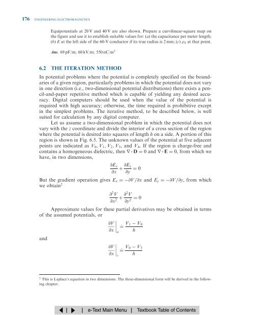
176 ENGINEERING ELECTROMAGNETICS
Equipotentials at 20 V and 40 V are also shown. Prepare a curvilinear-square map on
the figure and use it to establish suitable values for: …a† the capacitance permeterlength;
…b† E at the left side of the 60-V conductor if its true radius is 2 mm; …c† S at that point.
Ans. 69 pF/m; 60 kV/m; 550 nC/m 2
6.2 THE ITERATION METHOD
In potential problems where the potential is completely specified on the boundaries
of a given region, particularly problems in which the potential does not vary
in one direction (i.e., two-dimensional potential distributions) there exists a pencil-and-paper
repetitive method which is capable of yielding any desired accuracy.
Digital computers should be used when the value of the potential is
required with high accuracy; otherwise, the time required is prohibitive except
in the simplest problems. The iterative method, to be described below, is well
suited forcalculation by any digital computer.
Let us assume a two-dimensional problem in which the potential does not
vary with the z coordinate and divide the interior of a cross section of the region
where the potential is desired into squares of length h on a side. A portion of this
region is shown in Fig. 6.5. The unknown values of the potential at five adjacent
points are indicated as V 0 ; V 1 ; V 2 ; V 3 , and V 4 . If the region is charge-free and
contains a homogeneous dielectric, then r D ˆ 0 and r E ˆ 0, from which we
have, in two dimensions,
@E x
@x ‡ @E y
@y ˆ 0
But the gradient operation gives E x ˆ @V=@x and E y ˆ @V=@y, from which
we obtain 2
@ 2 V
@x 2 ‡ @2 V
@y 2 ˆ 0
Approximate values for these partial derivatives may be obtained in terms
of the assumed potentials, or
@V
@x _ˆ V1 V 0
a h
and
@V
@x
_ˆ V0 V 3
c h
2 This is Laplace's equation in two dimensions. The three-dimensional form will be derived in the following
chapter.