Chapter 6 Experimental Mapping Method
Chapter 6 Experimental Mapping Method
Chapter 6 Experimental Mapping Method

You also want an ePaper? Increase the reach of your titles
YUMPU automatically turns print PDFs into web optimized ePapers that Google loves.
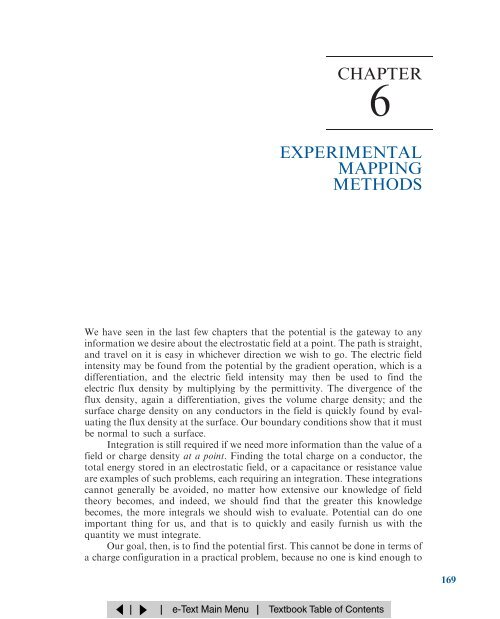
CHAPTER<br />
6<br />
EXPERIMENTAL<br />
MAPPING<br />
METHODS<br />
We have seen in the last few chapters that the potential is the gateway to any<br />
information we desire about the electrostatic field at a point. The path is straight,<br />
and travel on it is easy in whichever direction we wish to go. The electric field<br />
intensity may be found from the potential by the gradient operation, which is a<br />
differentiation, and the electric field intensity may then be used to find the<br />
electric flux density by multiplying by the permittivity. The divergence of the<br />
flux density, again a differentiation, gives the volume charge density; and the<br />
surface charge density on any conductors in the field is quickly found by evaluating<br />
the flux density at the surface. Our boundary conditions show that it must<br />
be normal to such a surface.<br />
Integration is still required if we need more information than the value of a<br />
field orcharge density at a point. Finding the total charge on a conductor, the<br />
total energy stored in an electrostatic field, or a capacitance or resistance value<br />
are examples of such problems, each requiring an integration. These integrations<br />
cannot generally be avoided, no matter how extensive our knowledge of field<br />
theory becomes, and indeed, we should find that the greater this knowledge<br />
becomes, the more integrals we should wish to evaluate. Potential can do one<br />
important thing for us, and that is to quickly and easily furnish us with the<br />
quantity we must integrate.<br />
Our goal, then, is to find the potential first. This cannot be done in terms of<br />
a charge configuration in a practical problem, because no one is kind enough to<br />
169
170 ENGINEERING ELECTROMAGNETICS<br />
tell us exactly how the charges are distributed. Instead, we are usually given<br />
several conducting objects or conducting boundaries and the potential difference<br />
between them. Unless we happen to recognize the boundary surfaces as belonging<br />
to a simple problem we have already disposed of, we can do little now and<br />
must wait until Laplace's equation is discussed in the following chapter.<br />
Although we thus postpone the mathematical solution to this important<br />
type of practical problem, we may acquaint ourselves with several experimental<br />
methods of finding the potential field. Some of these methods involve special<br />
equipment such as an electrolytic trough, a fluid-flow device, resistance paper<br />
and the associated bridge equipment, or rubber sheets; others use only pencil,<br />
paper, and a good supply of erasers. The exact potential can neverbe determined,<br />
but sufficient accuracy for engineering purposes can usually be attained.<br />
One othermethod, called the iteration method, does allow us to achieve any<br />
desired accuracy for the potential, but the number of calculations required<br />
increases very rapidly as the desired accuracy increases.<br />
Several of the experimental methods to be described below are based on an<br />
analogy with the electrostatic field, rather than directly on measurements on this<br />
field itself.<br />
Finally, we cannot introduce this subject of experimental methods of finding<br />
potential fields without emphasizing the fact that many practical problems<br />
possess such a complicated geometry that no exact method of finding that field is<br />
possible or feasible and experimental techniques are the only ones which can be<br />
used.<br />
6.1 CURVILINEAR SQUARES<br />
Our first mapping method is a graphical one, requiring only pencil and paper.<br />
Besides being economical, it is also capable of yielding good accuracy if used<br />
skillfully and patiently. Fair accuracy (5 to 10 percent on a capacitance determination)<br />
may be obtained by a beginnerwho does no more than follow the few<br />
rules and hints of the art.<br />
The method to be described is applicable only to fields in which no variation<br />
exists in the direction normal to the plane of the sketch. The procedure is<br />
based on several facts we have already demonstrated:<br />
1. A conductor boundary is an equipotential surface.<br />
2. The electric field intensity and electric flux density are both perpendicular to<br />
the equipotential surfaces.<br />
3. E and D are therefore perpendicular to the conductor boundaries and possess<br />
zero tangential values.<br />
4. The lines of electric flux, or streamlines, begin and terminate on charge and<br />
hence, in a charge-free, homogeneous dielectric, begin and terminate only on<br />
the conductorboundaries.
EXPERIMENTAL MAPPING METHODS 171<br />
Let us consider the implications of these statements by drawing the streamlines<br />
on a sketch which already shows the equipotential surfaces. In Fig. 6:1a two<br />
conductor boundaries are shown, and equipotentials are drawn with a constant<br />
potential difference between lines. We should remember that these lines are only<br />
the cross sections of the equipotential surfaces, which are cylinders (although not<br />
circular), since no variation in the direction normal to the surface of the paper is<br />
permitted. We arbitrarily choose to begin a streamline, or flux line, at A on the<br />
surface of the more positive conductor. It leaves the surface normally and must<br />
cross at right angles the undrawn but very real equipotential surfaces between the<br />
conductor and the first surface shown. The line is continued to the other conductor,<br />
obeying the single rule that the intersection with each equipotential must<br />
be square. Turning the paper from side to side as the line progresses enables us to<br />
maintain perpendicularity more accurately. The line has been completed in Fig.<br />
6:1b:<br />
In a similar manner, we may start at B and sketch anotherstreamline<br />
ending at B 0 . Before continuing, let us interpret the meaning of this pair of<br />
streamlines. The streamline, by definition, is everywhere tangent to the electric<br />
field intensity or to the electric flux density. Since the streamline is tangent to the<br />
electric flux density, the flux density is tangent to the streamline and no electric<br />
flux may cross any streamline. In other words, if there is a charge of 5 mC on the<br />
surface between A and B (and extending 1 m into the paper), then 5 mC of flux<br />
begins in this region and all must terminate between A 0 and B 0 . Such a pairof<br />
lines is sometimes called a flux tube, because it physically seems to carry flux<br />
from one conductor to another without losing any.<br />
We now wish to construct a third streamline, and both the mathematical<br />
and visual interpretations we may make from the sketch will be greatly simplified<br />
if we draw this line starting from some point C chosen so that the same amount<br />
of flux is carried in the tube BC as is contained in AB. How do we choose the<br />
position of C?<br />
FIGURE 6.1<br />
…a† Sketch of the equipotential surfaces between two conductors. The increment of potential between each<br />
of the two adjacent equipotentials is the same. …b† One flux line has been drawn from A to A 0 , and a second<br />
from B to B 0 :
172 ENGINEERING ELECTROMAGNETICS<br />
The electric field intensity at the midpoint of the line joining A to B may be<br />
found approximately by assuming a value for the flux in the tube AB, say C,<br />
which allows us to express the electric flux density by C=L t , where the depth<br />
of the tube into the paperis 1 m and L t is the length of the line joining A to B.<br />
The magnitude of E is then<br />
E ˆ 1 C<br />
L t<br />
However, we may also find the magnitude of the electric field intensity by<br />
dividing the potential difference between points A and A 1 , lying on two adjacent<br />
equipotential surfaces, by the distance from A to A 1 . If this distance is designated<br />
L N and an increment of potential between equipotentials of V is assumed,<br />
then<br />
E ˆ V<br />
L N<br />
This value applies most accurately to the point at the middle of the line<br />
segment from A to A 1 , while the previous value was most accurate at the midpoint<br />
of the line segment from A to B. If, however, the equipotentials are close<br />
together(V small) and the two streamlines are close together (C small), the<br />
two values found for the electric field intensity must be approximately equal,<br />
1 C<br />
ˆ V<br />
L t L N<br />
Throughout our sketch we have assumed a homogeneous medium ( constant),<br />
a constant increment of potential between equipotentials (V constant),<br />
and a constant amount of flux pertube (C constant). To satisfy all these<br />
conditions, (1) shows that<br />
…1†<br />
L t<br />
ˆ constant ˆ 1 C<br />
L N V<br />
…2†<br />
A similar argument might be made at any point in our sketch, and we are<br />
therefore led to the conclusion that a constant ratio must be maintained between<br />
the distance between streamlines as measured along an equipotential, and the<br />
distance between equipotentials as measured along a streamline. It is this ratio<br />
which must have the same value at every point, not the individual lengths. Each<br />
length must decrease in regions of greater field strength, because V is constant.<br />
The simplest ratio we can use is unity, and the streamline from B to B 0<br />
shown in Fig. 6:1b was started at a point for which L t ˆ L N . Since the ratio<br />
of these distances is kept at unity, the streamlines and equipotentials divide the<br />
field-containing region into curvilinear squares, a term implying a planar geometric<br />
figure which differs from a true square in having slightly curved and<br />
slightly unequal sides but which approaches a square as its dimensions decrease.
EXPERIMENTAL MAPPING METHODS 173<br />
Those incremental surface elements in our three coordinate systems which are<br />
planar may also be drawn as curvilinear squares.<br />
We may now rapidly sketch in the remainder of the streamlines by keeping<br />
each small box as square as possible. The complete sketch is shown in Fig. 6.2.<br />
The only difference between this example and the production of a field map<br />
using the method of curvilinear squares is that the intermediate potential surfaces<br />
are not given. The streamlines and equipotentials must both be drawn on an<br />
original sketch which shows only the conductor boundaries. Only one solution is<br />
possible, as we shall prove later by the uniqueness theorem for Laplace's equation,<br />
and the rules we have outlined above are sufficient. One streamline is<br />
begun, an equipotential line is roughed in, another streamline is added, forming<br />
a curvilinear square, and the map is gradually extended throughout the desired<br />
region. Since none of us can ever expect to be perfect at this, we shall soon find<br />
that we can no longer make squares and also maintain right-angle corners. An<br />
error is accumulating in the drawing, and our present troubles should indicate<br />
the nature of the correction to make on some of the earlier work. It is usually<br />
best to start again on a fresh drawing, with the old one available as a guide.<br />
The construction of a useful field map is an art; the science merely furnishes<br />
the rules. Proficiency in any art requires practice. A good problem for beginners<br />
is the coaxial cable or coaxial capacitor, since all the equipotentials are circles,<br />
while the flux lines are straight lines. The next sketch attempted should be two<br />
parallel circular conductors, where the equipotentials are again circles, but with<br />
different centers. Each of these is given as a problem at the end of the chapter,<br />
and the accuracy of the sketch may be checked by a capacitance calculation as<br />
outlined below.<br />
Fig. 6.3 shows a completed map fora cable containing a square inner<br />
conductor surrounded by a circular conductor. The capacitance is found from<br />
C ˆ Q=V 0 by replacing Q by N Q Q ˆ N Q C, where N Q is the numberof flux<br />
tubes joining the two conductors, and letting V 0 ˆ N V V, where N V is the<br />
number of potential increments between conductors,<br />
C ˆ NQQ<br />
N V V<br />
FIGURE 6.2<br />
The remainder of the streamlines have been added to Fig.<br />
6:1b by beginning each new line normally to the conductor<br />
and maintaining curvilinear squares throughout the sketch.
174 ENGINEERING ELECTROMAGNETICS<br />
FIGURE 6.3<br />
An example of a curvilinear-square field map.<br />
The side of the square is two thirds the radius<br />
of the circle. N V ˆ 4 and N Q ˆ 8 3:25 26,<br />
and therefore C ˆ 0 N Q =N V ˆ 57:6 pF/m.<br />
and then using (2),<br />
C ˆ NQ<br />
N V<br />
L t<br />
L N<br />
ˆ N Q<br />
N V<br />
…3†<br />
since L t =L N ˆ 1. The determination of the capacitance from a flux plot<br />
merely consists of counting squares in two directions, between conductors and<br />
around either conductor. From Fig. 6.3 we obtain<br />
8 3:25<br />
C ˆ 0 ˆ 57:6 pF=m<br />
4<br />
Ramo, Whinnery, and Van Duzer have an excellent discussion with examples<br />
of the construction of field maps by curvilinear squares. They offer the<br />
following suggestions: 1<br />
1. Plan on making a numberof rough sketches, taking only a minute orso<br />
apiece, before starting any plot to be made with care. The use of transparent<br />
paper over the basic boundary will speed up this preliminary sketching.<br />
2. Divide the known potential difference between electrodes into an equal<br />
numberof divisions, say fouroreight to begin with.<br />
1 By permission from S. Ramo, J. R. Whinnery, and T. Van Duzer, pp. 51±52. See Suggested References at<br />
the end of Chap. 5. Curvilinear maps are discussed on pp. 50±52.
EXPERIMENTAL MAPPING METHODS 175<br />
3. Begin the sketch of equipotentials in the region where the field is known best,<br />
as for example in some region where it approaches a uniform field. Extend<br />
the equipotentials according to your best guess throughout the plot. Note<br />
that they should tend to hug acute angles of the conducting boundary and be<br />
spread out in the vicinity of obtuse angles of the boundary.<br />
4. Draw in the orthogonal set of field lines. As these are started, they should<br />
form curvilinear squares, but, as they are extended, the condition of orthogonality<br />
should be kept paramount, even though this will result in some<br />
rectangles with ratios other than unity.<br />
5. Look at the regions with poor side ratios and try to see what was wrong with<br />
the first guess of equipotentials. Correct them and repeat the procedure until<br />
reasonable curvilinear squares exist throughout the plot.<br />
6. In regions of low field intensity, there will be large figures, often of five or six<br />
sides. To judge the correctness of the plot in this region, these large units<br />
should be subdivided. The subdivisions should be started back away from<br />
the region needing subdivision, and each time a flux tube is divided in half,<br />
the potential divisions in this region must be divided by the same factor.<br />
\ D6.1. Figure 6.4 shows the cross section of two circular cylinders at potentials of 0 and<br />
60 V. The axes are parallel and the region between the cylinders is air-filled.<br />
FIGURE 6.4<br />
See Prob. D6.1.
176 ENGINEERING ELECTROMAGNETICS<br />
Equipotentials at 20 V and 40 V are also shown. Prepare a curvilinear-square map on<br />
the figure and use it to establish suitable values for: …a† the capacitance permeterlength;<br />
…b† E at the left side of the 60-V conductor if its true radius is 2 mm; …c† S at that point.<br />
Ans. 69 pF/m; 60 kV/m; 550 nC/m 2<br />
6.2 THE ITERATION METHOD<br />
In potential problems where the potential is completely specified on the boundaries<br />
of a given region, particularly problems in which the potential does not vary<br />
in one direction (i.e., two-dimensional potential distributions) there exists a pencil-and-paper<br />
repetitive method which is capable of yielding any desired accuracy.<br />
Digital computers should be used when the value of the potential is<br />
required with high accuracy; otherwise, the time required is prohibitive except<br />
in the simplest problems. The iterative method, to be described below, is well<br />
suited forcalculation by any digital computer.<br />
Let us assume a two-dimensional problem in which the potential does not<br />
vary with the z coordinate and divide the interior of a cross section of the region<br />
where the potential is desired into squares of length h on a side. A portion of this<br />
region is shown in Fig. 6.5. The unknown values of the potential at five adjacent<br />
points are indicated as V 0 ; V 1 ; V 2 ; V 3 , and V 4 . If the region is charge-free and<br />
contains a homogeneous dielectric, then r D ˆ 0 and r E ˆ 0, from which we<br />
have, in two dimensions,<br />
@E x<br />
@x ‡ @E y<br />
@y ˆ 0<br />
But the gradient operation gives E x ˆ @V=@x and E y ˆ @V=@y, from which<br />
we obtain 2<br />
@ 2 V<br />
@x 2 ‡ @2 V<br />
@y 2 ˆ 0<br />
Approximate values for these partial derivatives may be obtained in terms<br />
of the assumed potentials, or<br />
@V<br />
@x _ˆ V1 V 0<br />
a h<br />
and<br />
@V<br />
@x<br />
_ˆ V0 V 3<br />
c h<br />
2 This is Laplace's equation in two dimensions. The three-dimensional form will be derived in the following<br />
chapter.
EXPERIMENTAL MAPPING METHODS 177<br />
FIGURE 6.5<br />
A portion of a region containing a twodimensional<br />
potential field, divided into<br />
squares of side h. The potential V 0 is<br />
approximately equal to the average of<br />
the potentials at the fourneighboring<br />
points.<br />
from which<br />
and similarly,<br />
Combining, we have<br />
or<br />
@V<br />
@ 2 <br />
V 0 @x<br />
@x 2 _ˆ<br />
<br />
<br />
a<br />
h<br />
@V<br />
@x<br />
<br />
<br />
c<br />
_ˆ V1 V 0 V 0 ‡ V 3<br />
h 2<br />
@ 2 V<br />
@y 2 0<br />
_ˆ V2 V 0 V 0 ‡ V 4<br />
h 2<br />
@ 2 V<br />
@x 2 ‡ @2 V<br />
@y 2 _ˆ V1 ‡ V 2 ‡ V 3 ‡ V 4 4V 0<br />
h 2 ˆ 0<br />
V 0 _ˆ 1<br />
4 …V 1 ‡ V 2 ‡ V 3 ‡ V 4 † …4†<br />
The expression becomes exact as h approaches zero, and we shall write it<br />
without the approximation sign. It is intuitively correct, telling us that the potential<br />
is the average of the potential at the four neighboring points. The iterative<br />
method merely uses (4) to determine the potential at the corner of every square<br />
subdivision in turn, and then the process is repeated over the entire region as<br />
many times as is necessary until the values no longer change. The method is best<br />
shown in detail by an example.<br />
For simplicity, consider a square region with conducting boundaries (Fig.<br />
6.6). The potential of the top is 100 V and that of the sides and bottom is zero.<br />
The problem is two-dimensional, and the sketch is a cross section of the physical<br />
configuration. The region is divided first into 16 squares, and some estimate of
178 ENGINEERING ELECTROMAGNETICS<br />
FIGURE 6.6<br />
Cross section of a square trough with sides and bottom at zero potential and top at 100 V. The cross<br />
section has been divided into 16 squares, with the potential estimated at every corner. More accurate<br />
values may be determined by using the iteration method.<br />
the potential must now be made at every corner before applying the iterative<br />
method. The betterthe estimate, the shorterthe solution, although the final<br />
result is independent of these initial estimates. When the computer is used for<br />
iteration, the initial potentials are usually set equal to zero to simplify the program.<br />
Reasonably accurate values could be obtained from a rough curvilinearsquare<br />
map, or we could apply (4) to the large squares. At the center of the figure<br />
the potential estimate is then 1 4<br />
…100 ‡ 0 ‡ 0 ‡ 0† ˆ25:0<br />
The potential may now be estimated at the centers of the four double-sized<br />
squares by taking the average of the potentials at the four corners or applying (4)<br />
along a diagonal set of axes. Use of this ``diagonal average'' is made only in<br />
preparing initial estimates. For the two upper double squares, we select a potential<br />
of 50 V forthe gap (the average of 0 and 100), and then V ˆ<br />
1<br />
4 …50 ‡ 100 ‡ 25 ‡ 0† ˆ43:8 (to the nearest tenth of a volt3 ), and forthe lower<br />
ones,<br />
V ˆ 1<br />
4<br />
…0 ‡ 25 ‡ 0 ‡ 0† ˆ6:2<br />
The potential at the remaining four points may now be obtained by applying (4)<br />
directly. The complete set of estimated values is shown in Fig. 6.6.<br />
The initial traverse is now made to obtain a corrected set of potentials,<br />
beginning in the upper left corner (with the 43.8 value, not with the boundary<br />
3 When rounding off a decimal ending exactly with a five, the preceding digit should be made even (e.g.,<br />
42.75 becomes 42.8 and 6.25 becomes 6.2). This generally ensures a random process leading to better<br />
accuracy than would be obtained by always increasing the previous digit by 1.
EXPERIMENTAL MAPPING METHODS 179<br />
where the potentials are known and fixed), working across the row to the right,<br />
and then dropping down to the second row and proceeding from left to right<br />
again. Thus the 43.8 value changes to 1 4<br />
…100 ‡ 53:2 ‡ 18:8 ‡ 0† ˆ43:0. The best<br />
or newest potentials are always used when applying (4), so both points marked<br />
43.8 are changed to 43.0, because of the evident symmetry, and the 53.2 value<br />
becomes 1 4<br />
…100 ‡ 43:0 ‡ 25:0 ‡ 43:0† ˆ52:8:<br />
Because of the symmetry, little would be gained by continuing across the<br />
top line. Each point of this line has now been improved once. Dropping down to<br />
the next line, the 18.8 value becomes<br />
V ˆ 1<br />
4<br />
…43:0 ‡ 25:0 ‡ 6:2 ‡ 0† ˆ18:6<br />
and the traverse continues in this manner. The values at the end of this traverse<br />
are shown as the top numbers in each column of Fig. 6.7. Additional traverses<br />
must now be made until the value at each corner shows no change. The values for<br />
the successive traverses are usually entered below each other in column form, as<br />
shown in Fig. 6.7, and the final value is shown at the bottom of each column.<br />
Only four traverses are required in this example.<br />
FIGURE 6.7<br />
The results of each of the four necessary traverses of the problem of Fig. 6.5 are shown in order in the<br />
columns. The final values, unchanged in the last traverse, are at the bottom of each column.
180 ENGINEERING ELECTROMAGNETICS<br />
FIGURE 6.8<br />
The problem of Figs. 6.6 and 6.7 is divided into smaller squares. Values obtained on the nine successive<br />
traverses are listed in order in the columns.
EXPERIMENTAL MAPPING METHODS 181<br />
If each of the nine initial values were set equal to zero, it is interesting to<br />
note that ten traverses would be required. The cost of having a computer do<br />
these additional traverses is probably much less than the cost of the programming<br />
necessary to make decent initial estimates.<br />
Since there is a large difference in potential from square to square, we<br />
should not expect our answers to be accurate to the tenth of a volt shown<br />
(and perhaps not to the nearest volt). Increased accuracy comes from dividing<br />
each square into four smaller squares, not from finding the potential to a larger<br />
number of significant figures at each corner.<br />
In Fig. 6.8, which shows only one of the symmetrical halves plus an additional<br />
column, this subdivision is accomplished, and the potential at the newly<br />
created corners is estimated by applying (4) directly where possible and diagonally<br />
when necessary. The set of estimated values appears at the top of each<br />
column, and the values produced by the successive traverses appear in order<br />
below. Here nine sets of values are required, and it might be noted that no values<br />
change on the last traverse (a necessary condition for the last traverse), and only<br />
one value changes on each of the preceding three traverses. No value in the<br />
bottom four rows changes after the second traverse; this results in a great saving<br />
in time, forif none of the fourpotentials in (4) changes, the answeris of course<br />
unchanged.<br />
For this problem, it is possible to compare our final values with the exact<br />
potentials, obtained by evaluating some infinite series, as discussed at the end of<br />
the following chapter. At the point for which the original estimate was 53.2, the<br />
final value for the coarse grid was 52.6, the final value for the finer grid was 53.6,<br />
and the final value fora 16 16 grid is 53.93 V to two decimals, using data<br />
obtained with the following Fortran program:<br />
1 DIMENSION A {17,17},B{17,17}<br />
2 DO 6 I=2,17<br />
3 DO 5 J=1,17<br />
4 A{I,J}=0.<br />
5 CONTINUE<br />
6 CONTINUE<br />
7 DO 9 J=2,16<br />
8 A{I,J}=100.<br />
9 CONTINUE<br />
10 A{1,1}=50.<br />
11 A{1,17}=50.<br />
12 DO 16 I=2,16<br />
13 DO 15 J=2,16<br />
14 A{I,J}={A{I,J-1}+A{I-1,J}+A{I,J+1}+A{I+1,J}}/4.<br />
15 CONTINUE<br />
16 CONTINUE<br />
17 DO 23 I=2,16<br />
18 DO 22 J=2,16
182 ENGINEERING ELECTROMAGNETICS<br />
19 C={A{I,J-1}+A{I-1,J}+A{I,J+1}+A{I+1,J}}/4.<br />
20 B{I,J}=A{I,J}-C<br />
21 IF{{ABS{B{I,J}}-.00001}.GT.0.} GO TO 12<br />
22 CONTINUE<br />
23 CONTINUE<br />
24 WRITE{6,25}{{A{I,J},J=1,17},I=1,17}<br />
25 FORMAT {1HO,17F7.2}<br />
26 STOP<br />
27 END<br />
Line 21 shows that the iteration is continued until the difference between successive<br />
traverses is less than 10 5 :<br />
The exact potential obtained by a Fourier expansion is 54.05 V to two<br />
decimals. Two other points are also compared in tabular form, as shown in<br />
Table 6.1.<br />
Computer flowcharts and programs for iteration solutions are given in<br />
Chap. 24 of Boast 4 and in Chap. 2 and the appendix of Silvester. 5<br />
Very few electrode configurations have a square or rectangular cross section<br />
that can be neatly subdivided into a square grid. Curved boundaries, acuteor<br />
obtuse-angled corners, reentrant shapes, and other irregularities require slight<br />
modifications of the basic method. An important one of these is described in<br />
Prob. 10 at the end of this chapter, and other irregular examples appear as Probs.<br />
7, 9, and 11.<br />
A refinement of the iteration method is known as the relaxation method. In<br />
general it requires less work but more care in carrying out the arithmetical steps. 6<br />
\ D6.2. In Fig. 6.9, a square grid is shown within an irregular potential trough. Using the<br />
iteration method to find the potential to the nearest volt, determine the final value at: …a†<br />
point a; …b† point b; …c† point c.<br />
Ans. 18V; 46V; 91V<br />
TABLE 6.1<br />
Original estimate 53:2 25.0 9.4<br />
4 4 grid 52.6 25.0 9.8<br />
8 8 grid 53.6 25.0 9.7<br />
16 16 grid 53.93 25.00 9.56<br />
Exact 54.05 25.00 9.54<br />
4 See Suggested References at the end of Chap. 2.<br />
5 See Suggested References at the end of this chapter.<br />
6 A detailed description appears in Scarborough, and the basic procedure and one example are in an earlier<br />
edition of Hayt. See Suggested References at the end of the chapter.
EXPERIMENTAL MAPPING METHODS 183<br />
FIGURE 6.9<br />
See Prob. D6.2.<br />
6.3 CURRENT ANALOGIES<br />
Several experimental methods depend upon an analogy between current density<br />
in conducting media and electric flux density in dielectric media. The analogy is<br />
easily demonstrated, for in a conducting medium Ohm's law and the gradient<br />
relationship are, for direct currents only,<br />
whereas in a homogeneous dielectric<br />
J ˆ E <br />
E ˆ rV <br />
D ˆ E <br />
E ˆ rV <br />
The subscripts serve to identify the analogous problems. It is evident that the<br />
potentials V and V , the electric field intensities E and E , the conductivity and<br />
permittivity and , and the current density and electric flux density J and D are<br />
analogous in pairs. Referring to a curvilinear-square map, we should interpret<br />
flux tubes as current tubes, each tube now carrying an incremental current which<br />
cannot leave the tube.<br />
Finally, we must look at the boundaries. What is analogous to a conducting<br />
boundary which terminates electric flux normally and is an equipotential surface?<br />
The analogy furnishes the answer, and we see that the surface must termi-
184 ENGINEERING ELECTROMAGNETICS<br />
nate current density normally and again be an equipotential surface. This is the<br />
surface of a perfect conductor, although in practice it is necessary only to use one<br />
whose conductivity is many times that of the conducting medium.<br />
Therefore, if we wished to find the field within a coaxial capacitor, which,<br />
as we have seen several times before, is a portion of the field of an infinite line<br />
charge, we might take two copper cylinders and fill the region between them<br />
with, for convenience, an electrolytic solution. Applying a potential difference<br />
betwen the cylinders, we may use a probe to establish the potential at any<br />
intermediate point, or to find all those points having the same potential. This<br />
is the essence of the electrolytic trough or tank. The greatest advantage of this<br />
method lies in the fact that it is not limited to two-dimensional problems.<br />
Practical suggestions for the construction and use of the tank are given in<br />
many places. 7<br />
The determination of capacitance from electrolytic-trough measurements is<br />
particularly easy. The total current leaving the more positive conductor is<br />
‡<br />
‡<br />
I ˆ J dS ˆ E dS<br />
S<br />
where the closed surface integral is taken over the entire conductor surface. The<br />
potential difference is given by the negative line integral from the less to the more<br />
positive plate,<br />
…<br />
V 0 ˆ E dL<br />
and the total resistance is therefore<br />
R ˆ V0<br />
I<br />
ˆ<br />
S<br />
„<br />
E dL<br />
† S E dS<br />
The capacitance is given by the ratio of the total charge to the potential<br />
difference,<br />
C ˆ Q ˆ † S E dS<br />
„<br />
V 0 E dL<br />
We now invoke the analogy by letting V 0 ˆ V 0 and E ˆ E . The result is<br />
RC ˆ <br />
<br />
…5†<br />
Knowing the conductivity of the electrolyte and the permittivity of the dielectric,<br />
we may determine the capacitance by a simple resistance measurement.<br />
A simplertechnique is available fortwo-dimensional problems. Conducting<br />
paper is used as the base on which the conducting boundaries are drawn with<br />
7 Weber is good. See Suggested References at the end of the chapter.
EXPERIMENTAL MAPPING METHODS 185<br />
silver paint. In the case of the coaxial capacitor, we should draw two circles of<br />
radii A and B ; B > A , extending the paint a small distance outward from B<br />
and inward from A to provide sufficient area to make a good contact with wires<br />
to an external potential source. A probe is again used to establish potential<br />
values between the circles.<br />
Conducting paper is described in terms of its sheet resistance R S . The sheet<br />
resistance is the resistance between opposite edges of a square. Since the fields are<br />
uniform in such a square, we may apply Eq. (13) from Chap. 5,<br />
R ˆ L<br />
S<br />
to the case of a square of conducting paper having a width w and a thickness t,<br />
where w ˆ L,<br />
R S ˆ L<br />
tL ˆ l<br />
t<br />
<br />
…6†<br />
Thus, if the conductive coating has a thickness of 0.2 mm and a conductivity of<br />
2 S/m, its surface resistance is 1=…2 0:2 10 3 †ˆ2500 . The units of R S are<br />
often given as ``ohms per square'' (but never as ohms per square meter).<br />
Fig. 6.10 shows the silver-paint boundaries that would be drawn on the<br />
conducting paper to determine the capacitance of a square-in-a-circle transmission<br />
line like that shown in Fig. 6.3. The generator and detector often operate at<br />
1 kHz to permit use of a more sensitive tuned detector or bridge.<br />
FIGURE 6.10<br />
A two-dimensional, two-conductor problem similar to that of Fig. 6.3 is drawn on conducting paper. The<br />
probe may be used to trace out an equipotential surface.
186 ENGINEERING ELECTROMAGNETICS<br />
\ D6.3. If the conducting papershown in Fig. 6.10 has a sheet resistance of 1800 per<br />
square, find the resistance that would be measured between the opposite edges of: …a† a<br />
square 9 cm on a side; …b† a square 4.5 cm on a side; …c† a rectangle 3 cm by 9 cm, across<br />
the longerdimension; …d† a rectangle 3 cm by 9 cm, across the shorter dimension. …e†<br />
What resistance would be measured between an inner circle of 0.8-cm radius and an<br />
outer circle of 2-cm radius?<br />
Ans. 1800 ; 1800 ; 5400 ; 600 ; 397 <br />
6.4 PHYSICAL MODELS<br />
The analogy between the electric field and the gravitational field was mentioned<br />
several times previously and may be used to construct physical models which are<br />
capable of yielding solutions to electrostatic problems of complicated geometry.<br />
The basis of the analogy is simply this: in the electrostatic field the potential<br />
difference between two points is the difference in the potential energy of unit<br />
positive charges at these points, and in a uniform gravitational field the difference<br />
in the potential energy of point masses at two points is proportional to their<br />
difference in height. In other words,<br />
W E ˆ QV<br />
W G ˆ Mgh<br />
…electrostatic†<br />
…gravitational†<br />
where M is the point mass and g is the acceleration due to gravity, essentially<br />
constant at the surface of the earth. For the same energy difference, then,<br />
V ˆ Mg h ˆ kh<br />
Q<br />
where k is the constant of proportionality. This shows the direct analogy between<br />
difference in potential and difference in elevation.<br />
This analogy allows us to construct a physical model of a known twodimensional<br />
potential field by fabricating a surface, perhaps from wood,<br />
whose elevation h above any point …x; y† located in the zero-elevation zeropotential<br />
plane is proportional to the potential at that point. Note that threedimensional<br />
fields cannot be handled.<br />
The field of an infinite line charge,<br />
V ˆ L<br />
2 ln B<br />
<br />
is shown on such a model in Fig. 6.11, which provides an accurate picture of the<br />
variation of potential with radius between A and B . The potential and elevation<br />
at B are conveniently set equal to zero.<br />
Such a model may be constructed for any two-dimensional potential field<br />
and enables us to visualize the field a little better. The construction of the models<br />
themselves is enormously simplified, both physically and theoretically, by the use<br />
of rubber sheets. The sheet is placed under moderate tension and approximates
EXPERIMENTAL MAPPING METHODS 187<br />
FIGURE 6.11<br />
A model of the potential field of an infinite line charge. The difference<br />
in potential is proportional to the difference in elevation.<br />
Contourlines indicate equal potential increments.<br />
closely the elastic membrane of applied mechanics. It can be shown 8 that the<br />
vertical displacement h of the membrane satisfies the second-order partial differential<br />
equation<br />
@ 2 h<br />
@x ‡ @2 h<br />
2 @y ˆ 0 2<br />
if the surface slope is small. We shall see in the next chapter that every potential<br />
field in a charge-free region also satisfies this equation, Laplace's equation in two<br />
dimensions,<br />
@ 2 V<br />
@x ‡ @2 V<br />
2 @y ˆ 0 2<br />
We shall also prove a uniqueness theorem which assures us that if a potential<br />
solution in some specified region satisfies the above equation and also gives<br />
the correct potential on the boundaries of this region, then this solution is the<br />
only solution. Hence we need only force the elevation of the sheet to corresponding<br />
prescribed potential values on the boundaries, and the elevation at all other<br />
points is proportional to the potential.<br />
For instance, the infinite-line-charge field may be displayed by recognizing<br />
the circular symmetry and fastening the rubber sheet at zero elevation around a<br />
circle by the use of a large clamping ring of radius B . Since the potential is<br />
constant at A , we raise that portion of the sheet to a greater elevation by<br />
pushing a cylinderof radius A up against the rubber sheet. The analogy breaks<br />
down for large surface slopes, and only a slight displacement at A is possible.<br />
The surface then represents the potential field, and marbles may be used to<br />
determine particle trajectories, in this case obviously radial lines as viewed<br />
from above.<br />
8 See, for instance, Spangenberg, pp. 75±76, in Suggested References at the end of the chapter.
188 ENGINEERING ELECTROMAGNETICS<br />
There is also an analogy between electrostatics and hydraulics that is particularly<br />
useful in obtaining photographs of the streamlines or flux lines. This<br />
process is described completely by Moore in a number of publications 9 which<br />
include many excellent photographs.<br />
\ D6.4. A potential field, V ˆ 200…x 2 4y ‡ 2† V, is illustrated by a plaster model with a<br />
scale of 1 vertical inch ˆ 400 V; the horizontal dimensions are true. The region shown is<br />
3 x 4m,0 y 1 m. In this region: …a† What is the maximum height of the model?<br />
…b† What is its minimum height? …c† What is the difference in height between points<br />
A…x ˆ 3:2; y ˆ 0:5† and B…3:8; 1†? …d† What angle does the line connecting these two<br />
points make with the horizontal?<br />
SUGGESTED REFERENCES<br />
1. Hayt, W. H., Jr.: ``Engineering Electromagnetics,'' 1st ed., McGraw-Hill<br />
Book Company, New York, 1958, pp. 150±152.<br />
2. Moore, A. D.: Fields from Fluid Flow Mappers, J. Appl. Phys., vol. 20, pp.<br />
790-804, August 1949; Soap Film and Sandbed MapperTechniques, J. Appl.<br />
Mech. (bound with Trans. ASME), vol. 17, pp. 291±298, September1950;<br />
Four Electromagnetic Propositions, with Fluid Mapper Verifications, Elec.<br />
Eng., vol. 69, pp. 607±610, July 1950; The Further Development of Fluid<br />
Mappers, Trans. AIEE, vol. 69, part II, pp. 1615±1624, 1950; <strong>Mapping</strong><br />
Techniques Applied to Fluid MapperPatterns, Trans. AIEE, vol. 71, part<br />
I, pp. 1±5, 1952.<br />
3. Salvadori, M. G., and M. L. Baron: ``Numerical <strong>Method</strong>s in Engineering,''<br />
2d ed., Prentice-Hall, Inc., Englewood Cliffs, N.J., 1961. Iteration and<br />
relaxation methods are discussed in chap. 1.<br />
4. Scarborough, J. B.: ``Numerical Mathematical Analysis,'' 6th ed., The Johns<br />
Hopkins Press, Baltimore, 1966. Describes iteration relaxation methods and<br />
gives several complete examples. Inherent errors are discussed.<br />
5. Silvester, P.: ``Modern Electromagnetic Fields,'' Prentice-Hall, Inc.,<br />
Englewood Cliffs, N.J., 1968.<br />
6. Soroka, W. W.: ``Analog <strong>Method</strong>s in Computation and Simulation,''<br />
McGraw-Hill Book Company, New York, 1954.<br />
7. Spangenberg, K. R.: ``Vacuum Tubes,'' McGraw-Hill Book Company, New<br />
York, 1948. <strong>Experimental</strong> mapping methods are discussed on pp. 75±82.<br />
8. Weber, E.: ``Electromagnetic Fields,'' vol. I, John Wiley & Sons, Inc., New<br />
York, 1950. <strong>Experimental</strong> mapping methods are discussed in chap. 5.<br />
9 See Suggested References at the end of this chapter.
EXPERIMENTAL MAPPING METHODS 189<br />
PROBLEMS<br />
6.1 Construct a curvilinear-square map for a coaxial capacitor of 3-cm inner<br />
radius and 8-cm outer radius. These dimensions are suitable for the<br />
drawing. …a† Use yoursketch to calculate the capacitance permeter<br />
length, assuming R ˆ 1. …b† Calculate an exact value forthe capacitance<br />
perunit length.<br />
6.2 Construct a curvilinear-square map of the potential field about two<br />
parallel circular cylinders, each of 2.5-cm radius, separated a center-tocenterdistance<br />
of 13 cm. These dimensions are suitable forthe actual<br />
sketch if symmetry is considered. As a check, compute the capacitance<br />
per meter both from your sketch and from the exact formula. Assume<br />
R ˆ 1:<br />
6.3 Construct a curvilinear-square map of the potential field between two<br />
parallel circular cylinders, one of 4-cm radius inside one of 8-cm radius.<br />
The two axes are displaced by 2.5 cm. These dimensions are suitable for<br />
the drawing. As a check on the accuracy, compute the capacitance per<br />
meter from the sketch and from the exact expression:<br />
2<br />
cosh 1 a 2 ‡ b 2 D 2<br />
2ab<br />
where a and b are the conductor radii and D is the axis separation.<br />
6.4 A solid conducting cylinder of 4-cm radius is centered within a rectangularconducting<br />
cylinderwith a 12-cm by 20-cm cross section. …a† Make<br />
a full-size sketch of one quadrant of this configuration and construct a<br />
curvilinear-square map for its interior. …b† Assume ˆ 0 and estimate C<br />
permeterlength.<br />
6.5 The innerconductorof the transmission line shown in Fig. 6.12 has a<br />
square cross section 2a 2a, while the outersquare is 5a 5a. The axes<br />
are displaced as shown. …a† Construct a good-sized drawing of this transmission<br />
line, say with a ˆ 2:5 cm, and then prepare a curvilinear-square<br />
plot of the electrostatic field between the conductors. …b† Use yourmap<br />
to calculate the capacitance permeterlength if ˆ 1:6 0 . …c† How would<br />
the answerto part b change if a ˆ 0:6 cm?<br />
6.6 Let the innerconductorof the transmission line shown in Fig. 6.12 be at<br />
a potential of 100 V, while the outer is at zero potential. Construct a grid,<br />
0:5a on a side, and use iteration to find V at a point that is a units above<br />
the upper right corner of the inner conductor. Work to the nearest volt.<br />
6.7 Use the iteration method to estimate the potential at points x and y in<br />
the triangular trough of Fig. 6.13. Work only to the nearest volt.<br />
6.8 Use iteration methods to estimate the potential at point x in the trough<br />
shown in Fig. 6.14. Working to the nearest volt is sufficient.<br />
6.9 Using the grid indicated in Fig. 6.15, work to the nearest volt to estimate<br />
the potential at point A:
190 ENGINEERING ELECTROMAGNETICS<br />
FIGURE 6.12<br />
See Probs. 5, 6, and 14.<br />
6.10 Conductors having boundaries that are curved or skewed usually do not<br />
permit every grid point to coincide with the actual boundary. Figure<br />
6.16a illustrates the situation where the potential at V 0 is to be estimated<br />
in terms of V 1 ; V 2 ; V 3 ; V 4 , and the unequal distances h 1 ; h 2 ; h 3 , and h 4 .<br />
…a† Show that<br />
V 1<br />
V 0 ˆ <br />
1 ‡ h 1<br />
1 ‡ h ‡<br />
1h 3<br />
h 3 h 4 h 2<br />
‡ <br />
1 ‡ h <br />
4<br />
h 2<br />
V 4<br />
<br />
<br />
V 2<br />
1 ‡ h 2<br />
1 ‡ h ‡<br />
2h 4<br />
h 4 h 4 h 3<br />
<br />
1 ‡ h <br />
3<br />
h 1<br />
1 ‡ h ; …b† determine V 0 in Fig. 6.16b:<br />
4h 2<br />
h 3 h 1<br />
V 3<br />
<br />
1 ‡ h <br />
3h 1<br />
h 2 h 4<br />
6.11 Consider the configuration of conductors and potentials shown in Fig.<br />
6.17. Using the method described in Prob. 10, write an expression for V 0
EXPERIMENTAL MAPPING METHODS 191<br />
FIGURE 6.13<br />
See Prob. 7.<br />
FIGURE 6.14<br />
See Prob. 8.
192 ENGINEERING ELECTROMAGNETICS<br />
FIGURE 6.15<br />
See Prob. 9.<br />
in terms of V 1 ; V 2 ; V 3 , and V 4 at point: …a† x; …b† y; …c† z. …d† Use the<br />
iteration method to estimate the potential at point x.<br />
6.12 …a† Afterestimating potentials forthe configuration of Fig. 6.18, use the<br />
iteration method with a square grid 1 cm on a side to find better estimates<br />
at the seven grid points. Work to the nearest volt. …b† Construct<br />
0.5-cm grid, establish new rough estimates, and then use the iteration<br />
method on the 0.5-cm grid. Again work to the nearest volt. …c† Use the<br />
computer to obtain values for a 0.25-cm grid. Work to the nearest 0.1 V.<br />
6.13 Perfectly conducting concentric spheres have radii of 2 and 6 cm. The<br />
region 2 < r < 3 cm is filled with a solid conducting material for which<br />
FIGURE 6.16<br />
See Prob. 10.
EXPERIMENTAL MAPPING METHODS 193<br />
FIGURE 6.17<br />
See Prob. 11.<br />
ˆ 100 S/m, while the portion for which 3 < r < 6 cm has ˆ 25 S/m.<br />
The innersphere is held at 1 V while the outeris at V ˆ 0. …a† Find E and<br />
J everywhere. …b† What resistance would be measured between the two<br />
spheres? …c† What is V at r ˆ 3 cm?<br />
6.14 The cross section of the transmission line shown in Fig. 6.12 is drawn on<br />
a sheet of conducting paperwith metallic paint. The sheet resistance is<br />
2000 persquare and the dimension a is 2 cm. …a† Assuming a result for<br />
Prob. 6b of 110 pF/m, what total resistance would be measured between<br />
the metallic conductors drawn on the conducting paper? …b† What would<br />
the total resistance be if a ˆ 2 cm?<br />
FIGURE 6.18<br />
See Prob. 12.
194 ENGINEERING ELECTROMAGNETICS<br />
FIGURE 6.19<br />
See Prob. 16.<br />
6.15 Two concentric annular rings are painted on a sheet of conducting paper<br />
with a highly conducting metallic paint. The four radii are 1, 1.2, 3.5, and<br />
3.7 cm. Connections made to the two rings show a resistance of 215 <br />
between them. …a† What is R S forthe conducting paper? …b† If the conductivity<br />
of the material used as the surface of the paper is 2 S/m, what is<br />
the thickness of the coating?<br />
6.16 The square washer shown in Fig. 6.19 is 2.4 mm thick and has outer<br />
dimensions of 2:5 2:5 cm and innerdimensions of 1:25 1:25 cm.<br />
The inside and outside surfaces are perfectly conducting. If the material<br />
has a conductivity of 6 S/m, estimate the resistance offered between the<br />
inner and outer surfaces (shown shaded in Fig. 6.19). A few curvilinear<br />
squares are suggested.<br />
6.17 A two-wire transmission line consists of two parallel perfectly conducting<br />
cylinders, each having a radius of 0.2 mm, separated a center-tocenter<br />
distance of 2 mm. The medium surrounding the wires has<br />
R ˆ 3 and ˆ 1:5 mS/m. A 100-V battery is connected between the<br />
wires. Calculate: …a† the magnitude of the charge per meter length on<br />
each wire; …b† the battery current.<br />
6.18 A coaxial transmission line is modelled by the use of a rubber sheet<br />
having horizontal dimensions that are 100 times those of the actual<br />
line. Let the radial coordinate of the model be m . Forthe line itself,<br />
let the radial dimension be designated by as usual; also, let a ˆ 0:6mm<br />
and b ˆ 4:8 mm. The model is 8 cm in height at the innerconductorand<br />
zero at the outer. If the potential of the inner conductor is 100 V: …a† find<br />
the expression for V…†. …b† Write the model height as a function of :