Final documentation of the CGERegEU+ model

Common Agricultural Policy Regional Impact – The Rural Development Dimension
Collaborative project - Small to medium-scale focused research project under the Seventh Framework Programme
Project No.: 226195
WP3.2 Model development and adaptation – Regional CGEs
Deliverable: D3.2.3
Final documentation of the CGERegEU+ model
DRAFT VERSION
Hannu Törmä, Katarzyna Zawalinska
University of Helsinki, Ruralia Institute
August 31 st , 2011
1

Contents
1 Introduction .................................................................................................................................. 3
2 Additions to the base model ......................................................................................................... 3
2.1 Dixon-Parmenter-Sutton-Vincent (DPSV) investment rule .................................................. 3
2.2 Balance of payment equations (EU co-financing of RD measures) ...................................... 6
3 Closures ........................................................................................................................................ 8
3.1 Automatic (technical) closure in Tablo ................................................................................. 8
3.2 Changes to the automatic closure ........................................................................................ 10
3.2.1 Swaps proposed in the closure ..................................................................................... 12
4 Modelling of RD measures ........................................................................................................ 12
4.1 Variables and shocks ........................................................................................................... 13
4.1.1 Modelling investments in human capital ..................................................................... 13
4.1.2 Subsidies for investments in physical capital .............................................................. 14
4.1.3 Direct income transfers ................................................................................................ 15
4.1.4 Land subsidies .............................................................................................................. 15
4.1.5 Subsidies for non-agricultural services in rural areas .................................................. 16
4.2 Parameterization of the shocks ............................................................................................ 16
4.2.1 Shocks for investment in human capital ...................................................................... 16
4.2.2 Shocks for investments in physical capital .................................................................. 16
4.2.3 Shocks for direct income transfers ............................................................................... 17
4.2.4 Shocks for land subsidies ............................................................................................. 17
4.2.5 Shocks for non-agricultural services in rural areas ...................................................... 17
5 Running the base model in GEMPACK .................................................................................... 18
5.1 GEMPACK sub-programs .................................................................................................. 18
5.2 Simulation setup in RunGEM ............................................................................................. 19
6 Conclusions and summary ......................................................................................................... 21
7 List of measures under 2007-2013 RDPs .................................................................................. 22
8 Bibliography............................................................................................................................... 23
2

1 Introduction
This paper documents how to use the CGERegEU model to simulate the Pillar II measures at the
NUTS 2 level for EU27+ countries. It starts with the update on the latest model‟s development after
the deliverable D.3.2.2. The most recent additions concern two aspects: improving the
characteristics of investments (i.e. introducing quasi dynamics in the comparative static model) and
featuring the external co-financing from the EU budget for the Pillar II measures (i.e. adding
balance of payment equations). Further, the paper explains: the possible choices for the model‟s
closures – depending on the policy focus (e.g. short run vs. long run, etc.). It also explains the
simulation design of the RD measures in terms of the variables and shocks implemented. Then it
includes a short manual on how to use the GEMPACK software in order to actually run the model
and produce robust results on the regional impact of Pillar II measures. The paper ends with
summary and conclusions as well as with model coding and electronic version of all essential files
needed to run the model.
2 Additions to the base model
In D3.2.2 we added four new features into the base model. They are: the land factor, different real
wage theories, the Stone-Geary utility function (instead of Cobb-Douglas) and public sector
accounting. Thanks to these additions we have now three primary production factors: labour,
capital, and land. Besides, now we can experiment with different wage theories: sticky wages,
adjusted Phillips curve or Wage curve based real wages. The Cobb-Douglas utility function has
been replaced with the Stone-Geary leading to Linear Expenditure System, which is more
sophisticated. Public sector accounting shows the tax revenues collected, and transfers given.
Comparing to the second deliverable two new features have been added to the model. First, the
investment rule allowing investment demands to be industry specific and endogenous, even if the
model is still comparative static in its nature. Second, balance of payment equations were
introduced to allow taking into account the external EU co-financing of the Pillar II measures from
the EARDF budget.
2.1 Dixon-Parmenter-Sutton-Vincent (DPSV) investment rule
Up till now investments have been exogenous. For our purposes, it is better to use a more advanced
investment rule, which is called DPSV (Dixon, Parmenter, Sutton, and Vincent, 1982, cp. 19).
According to this theory, investments made during a year can affect the capital stock of the same
year. We begin by presenting a conventional investment-capital stock flow mechanism. Small
letters indicate percentage changes.
xcap 1 = xinv 1 + (1 – δ) xcap 0 (all i, r)
xcap 0 and xcap 1 refer to the capital stock at the beginning and end of the same year, xinv 1 is
investment or creation of new capital goods during the year, and δ is the rate of depreciation, wear
3

and tear of the capital stock. The new capital goods xinv 1 are assumed to be produced according to
the Leontief structure from domestic inputs.
The only things that affect the capital stock at the end of one year are the current capital stock,
depreciation and investment. It is thus assumed that the effects of past investment decisions are
fully incorporated in the current capital stock.
The theory do not attempt to explain total investments, only how this investment is allocated across
using industries after a change in economic conditions. It is assumed that there is an existing macro
economic policy that determines their size.
The current gross rate of return on fixed capital in a sector, gret is defined as the ratio of the capital
rent, pcap and the cost of a unit of investment, pinv. Net rate of return is received by subtracting the
rate of depreciation of capital.
gret = pcap - pinv
nret = gret - δ
(all i,r)
The gross rate of return or profitability will increase (decrease) if the capital rent increases
(decreases) more (less) than investment costs. Increasing profitability implies that the firms are
earning more capital income than they pay as investment costs. We further assume that capital in a
sector takes one year to install.
Investors are assumed to be cautious in assessing the effects of expanding the capital stock in a
sector. They behave as if they expect that sector‟s rate of return schedule in one year‟s time have
the following form.
gret 1 = gret 0 - β (xcap 1 - xcap 0 )
(all i,r)
0 and 1 represent the situation at the beginning and end of same year, and β is a positive parameter.
The schedule is in the following figure.
4

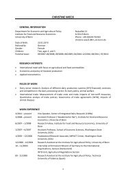
Figure 1 Expected rate of return schedule for a sector (Dixon et al., 1982)
The horizontal axis measures the difference between the future and current capital stocks, measured
as percentage points. The vertical axis shows the expected rate of return. If the capital stock were
maintained at the existing level, then the expected rate of return would be the current rate of return,
gret 0 . However, if investment plans were set so that xcap 1 – xcap 0 would reach the level A, then
businessmen would behave as if they espected the rate of return to fall to B.
Now we assume that total investment expenditure, xinv_ir is allocated across industries so as to
equate the expected rates of return. This means that there exists some rate of return ω such that
-β (xcap 1 - xcap 0 ) gret 0 = ω (all i,r)
The gross growth rate of capital, ggro in a sector increases (decreases) if the gross rate of return of
that sector is larger (smaller) than the economy-wide rate of return ω. This indicates that
investments grom faster that the capital stock within one year.
ggro = xinv – xcap
(all i,r)
After substitutions of the above equations we get an equation for the gross growth rate of capital.
ggro = finv + 0.33 (2.0 gret – invslack)
(all i,r)
finv is a shifter to enforce DSPV investment rule, 0.33 is 1/β, 2.0 is the ratio of gross to net rate of
return and invslack corresponds to ω, the exogenous economy-wide rate of return. It is to be
interpreted as a risk related relationship with relatively fast- (slow-) growing industries requiring
premia (accepting discounts) on their rates of return. According to Horridge (2003) attempts to
improve the theory by updating these parameter values have been found to occasionally lead to
perversely signed coefficients.
5

Considering the conventional investment-capital stock flow mechanism (see above), total
investment expenditure is as follows.
xinv_ir = ∑ i,r pinv xinv
(all i,r)
The DPSV rule relates for most sectors the investment of each sector to profitability in that sector.
The effect is that sectors which become more profitable attract more investment. In some sectors,
like in those where investment is determined by government policy, this rule might be
inappropriate. In these sectors investments are not mainly driven by current profits, like in
education, administration etc. For this kind of sectors, it is better to let investment follow aggregate
investment or national/regional trend (Horridge, 2003).
2.2 Balance of payment equations (EU co-financing of RD measures)
Since Pillar II measures are at least partly financed by EU (usually 75% to 80%) we need to take it
into account in our model because the outcomes of the policy differ depending on the source of its
financing (domestic vs. foreign financing). If the policy is fully financed domestically, the spending
has to be covered through savings/earnings obtained elsewhere in the domestic economy (e.g. from
increased government revenues from higher taxes). It is different if the financing comes from
outside of the economy, from abroad (e.g. EU budget 1 ) then it affects the country‟s position vis-avis
the rest of the world. Hence it affects the Balance of payments (BOP) accounts, which is a
record of all monetary transactions between a country and the rest of the world.
In the long run, all components of the BOP accounts must sum to zero with no overall surplus or
deficits because all debts have to be paid. Thus, the current account on one side and the capital and
financial account on the other should balance each other out. When an economy, however, has
positive capital and financial accounts (a net financial inflow), the country's debits are more than its
credits (due to an increase in liabilities to other economies or a reduction of claims in other
countries). This is usually in parallel with a current account (trade) deficit; an inflow of money
means that the return on an investment is a debit on the current account. Thus, the economy is using
world savings to meet its local investment and consumption demands. It is a net debtor to the rest of
the world. This is the case of co-financing of RD measures, where the contributions from the
European Agricultural Fund for Rural Development (EAFRD) are counted as capital inflows. That
is why we allow in the model the balance of trade (BOT) moving towards the deficit by the value of
the EAFRD contributions to Pillar II measures, in order to counterbalance BOP.
The following variables and equations were added to the model in order to take account of the BOP
balancing:
1 Of course it has not to be forgotten that countries pay contributions to the EU budget anyway, and some are net
creditors while other are net debtors towards the CAP policy in general.
6

Balance of trade is the difference between the value of total exports and imports to/from the rest of
the world (ROW).
BOT = ∑ r VROWEXPtot - ∑ r VROWIMPtot
The ratio of the BOT to the value of the expenditure side GDP is of the following form.
R_BOT_GDP = BOT / ∑ r GDPEXP
The percentage change in the BOT, d_bot is defined as follows.
100 * d_bot = ∑ r VROWEXPtot* (xrowexp_cr + prowexp_cr)
- ∑ r VROWIMPtot* (xrowimp_cr + prowimp_cr)
xrowexp_cr and xrowimp_cr are percentage changes of national exports, and prowexp_cr and
prowimp_cr are the corresponding prices. The variables on the parenthes are endogenous, so d_bot
will change according to their adjustment.
The percentage change in the BOT/GDP ratio depends on:
(100 / R_BOT_GDP) * d_bot_gdp = (100 / BOT) * d_bot – wgdpexp_r
Here wgdpexp_r is national nominal expenditure side GDP.
It is important to mention that in case of inflow of euros to the economies which have other than
euro currencies (e.g. zloty in Poland, koruna in Czech Republic, etc.) the inflow makes a pressure
on appreciation of the domestic currencies (prowimp), since euro have to be exchanged into
national currency which increases the demand for it.
Taking into account external co-financing from EARDF requires establishing the following shock
statement in the command file:
Shock d_bot = - x;
where x equals to amount of co-financing from EARDF in mln of national currency. As explained
before, the shock is negative, because percentage change of the balance of trade (d_bot) has to be
put into deficit in order to counterbalance the financial inflows.
7

3 Closures
One important feature of the base model implemented in the GEMPACK software is its ability to
set up closures specific for each policy simulations which can be changed (adjusted) in order to
reflect the reality in the model well as possible. In other words, the choice of closure in CGE model
determines the choice of macroeconomic theory used in simulation and also decides about the
causalities leading to the particular results (Taylor i von Arnim, 2007]. Technically the closure of
the model for a particular simulation specified which variables are exogenous (that is, their values
are given as shocks are unchanged in levels) and which variables are endogenous (that is, the
variable calculated when the model is solved).
3.1 Automatic (technical) closure in Tablo
Technically, the number of endogenous variables in a CGE model must equal the number of
equations. For complex models with thousands of equations and variables having various
dimensions (multi regions, sectors, factors, etc.) it is a very demanding task to find a sensible
closure, which satisfies this accounting restriction. That is why GEMPACK provides a technical
check up and offers a list of all unmatched (without equations) variables which are most probably
exogenous (the rest is assumed endogenous) 2 . The automatic closure for CGERegEU+ is provided
as follows.
Table 1 Automatic closure for CGERegEU+
! Automatic closure generated by TABmate Tools...Closure command
Variable / Dimension
Exogenous acap ; ! IND*REG Capital-augmenting technical change
Exogenous alab ; ! IND*REG Labor-augmenting technical change
Exogenous aland ; ! IND*REG Land-augmenting technical change
Exogenous aprim ; ! IND*REG Primary-factor-augmenting tech change
Exogenous atot ; ! IND*REG All-input-augmenting technical change
Exogenous
Exogenous
ahou_s ; ! COM*REG Taste change, househ. imp/dom composite
fhou ; ! REG Reg. aver. propen. to cons. from disp income
Exogenous delCAPTAXRATE ; ! IND*REG Change, capital tax rate
Exogenous delHOUTAXRATE ; ! REG Tax rate, Arm and ROF goods to hou
Exogenous delLABTAXRATE ; ! IND*REG Change, labour tax rate
Exogenous delLANDTAXRATE ; ! IND*REG Change, land tax rate
Exogenous delPRDTAXRATE ; ! IND*REG Change, prod tax rate
Exogenous thouloc ; ! REG Local income tax rate
Exogenous thoustate ; ! REG National income tax rate
Exogenous fgov ; ! COM*GVT*REG Gov. demand shift variable
Exogenous fgov_c ; ! GVT*REG Gov. demand shift variable
Exogenous fgov_cgr ; ! 1 Gov. demand shift variable
Exogenous fgov_cr ; ! GVT Gov. demand shift variable
Exogenous fhou_r ; ! 1 Economy-wide shift on regional APCs
Exogenous finv1 ; ! IND*REG Investment shift variable
Exogenous flab ; ! IND*REG Real wage shifter
2 Technically, authomatic closure is available from TABMATE in Tools/Tablo make code/Closure.
8

Exogenous flab_i ; ! REG Real wage shifter
Exogenous flab_ir ; ! 1 Real wage shifter
Exogenous flab_r ; ! IND Real wage shifter
Exogenous fstatehou ; ! REG Shifter-transf. from nat. gov to reg. hou.
Exogenous fstateloc ; ! REG Shifter: transfers from nat. to reg. gov
Exogenous fstateloc_r ; ! 1 Shifter: transfers from nat. to reg. gov
Exogenous fxserr ; ! COM*REG Xserr shift variable
Exogenous invslack ; ! 1 Invest. slack for exogenizing nat. invest
Exogenous nhou ; ! REG Number of households
Exogenous prowexp ; ! COM Price, exports to ROW, National currency
Exogenous prowimp ; ! 1 Price of imports, National currency
Exogenous xcap ; ! IND*REG Quantity of capital demanded
Exogenous xhoutot ; ! REG Real Spending by households
Exogenous xirof ; ! ROF*REG ROF goods used by investment
Exogenous xirow ; ! REG ROW goods for investment
Exogenous xland ; ! IND*REG Quantity of land (resource) demanded
Rest endogenous; ! end of TABmate automatic closure
The first block of the exogenous variables (Table1) covers all technical change variables which are
usually exogenous as in CGERegEU+ (unless the model has built in the endogenous growth theory
in it). There are several input-augmenting technical change variables for individual or grouped
inputs, i.e. labor-augmenting technical change (alab), capital-augmenting technical change (acap),
land-augmenting technical change (aland), and also combined input technical changes, i.e.primaryfactor-augmenting
technical change (aprim) and all-input-augmenting technical change (atot). In
case of all technical change variable, the negative shock means that the technology improved in
terms of the particular input, so less of the input is needed to obtain the same amount of output than
before (the whole isoquant shifts).
Apart from technical variables also the taste variable is included (ahou_s) and the propensity to
consume which both are naturally set up outside of the model, at least in the short run closure. The
next block of exogenous variables consists of the tax rates both indirect (on labour, land, capital,
goods and production) and direct (local and national income tax). Since those variables are policy
tools they naturally come as exogenous in the model.
Another exogenous block of variables covers a broad range of shifters. Shift variables are ones that
are originally exogenous and they are used in order to switch on or off certain equations in order to
choose which variant of the theory we want to follow. For example in the labour market block there
is one real wage equation per wage theory, with labour shifters. Three wage theories offer a choice
between sticky wages in the short run vs fully adjustable nominal wages along wage curve (see the
equations explained in D3.2.2). There are real wage shifters (flab shifters) in all real wage theories
with different sectoral and regional dimensions. Consider the first theory. When the shifters are
exogenous their value will be zero. In this case nominal wage follow inflation, so real wage is
sticky. The assumption is the third theory where the change of the unemployment rate and real
wage are determined jointly. In similar fashion work other shifters - in equations for distribution of
government demand, for transfers from government to households, for exogenising national
investment, etc.
9

Further, the number of households is exogenous as well as reference prices (in national currency) -
prowimp - price of imports (numeraire), and prowexp – price of exports. Their exogeneity comes
from the small open economy assumption. Last but not least, the block of certain quantity variables
is exogenous. They include: quantity of capital and land demanded, real spending by households
(from LES), goods used by investment including imported goods to it.
3.2 Changes to the automatic closure
There is no unique or proper closure, on the other hand closure needs to be justifiable. Basically
there are three reasons for which we alter the automatic closure: 1) to take account of the time
horizon of the simulations (short vs. long run closure), 2) to take account of the macroeconomic
features of analysed economies (e.g. small open economy vs. big open economy), 3) to allow
particular policy simulations.
The typical short run closure in a comparative static model assumes that employment is endogenous
while capital and land are exogenous. Wages in short run are usually assumed to be sticky - little
responsiveness due to wage contracts, labour union negotiations, etc.. Rate of return on capital is
endogenous. Trade balance is endogenous but the remaining composites of GDP expenditure side
(private and public consumption) are exogenous (Figure 1).
Figure 1 Typical causation in short-run closure in a comparative-static model
Source: OraniG course materials by CoPS, Monash University Melbourne Australia
10

On the contrary the long run closure assumes that employment is exogenous (does not depend on
policy but demographic determinants) and determines real wage. Capital stock is endogenous and
depends on rate of return on capital. If DPSV (or other endogenization of investment rule) is
included, then sectoral investment follows capital. Land can be sometimes endogenous in the long
run as well (if there are some reserves in some types of land and if land supply is responsive to
policy measures) or exogenous as usually it is a case. Trade balance is exogenous in long run while
other elements of national absorption are endogenous (public and private consumption and
investments).
Figure 2 Typical causation in the long-run closure in a comparative-static model
Source: OraniG course materials by CoPS, Monash University Melbourne Australia
Typically, macro-environment in the closure refers to macroeconomic determinants (theories) for
particular economies. It includes also relations of the economy vis-a-vis the rest of the world. If the
economy is small it cannot affect the rest of the world prices, so price of exports and also price of
imports are exogenous. In the short run a country can run on deficit on the trade account which
represents national dissaving, so balance of trade can be endogenous. However, no country can run
the trade deficit constantly, so in the long run it is natural to fix the balance of trade so it becomes
exogenous. Besides, if the policy is financed from abroad, the trade balance is affected so it is
exogenised to be shocked by the amount of the external financing. Macro-environment can also
specify which wage theory is used (sticky wages or wage curve, etc.) and other economic theories.
11

Simulations can specifically require some exogenisation of certain variables to shock them or
endogenisation to see the effect on them. For example in case of direct transfers to households (as in
case of early retirement scheme) they are initially endogenous but since we know the amounts
transferred to them we exogenise them so to shock them and then see the policy effects.
3.2.1 Swaps proposed in the closure
All the changes to the automatic closure are done by swapping the initially exogenous variables
with the presently endogenous ones. The following swaps are proposed for our simulations and as
such are the part of the command file (below the automatic closure):
1) Time horizon swaps
! Long-run factor market closure
swap xcap = fgret; ! Capital stock determined endogenously
swap finv1 = ggro; ! Investment follows xcap
swap flab_ir = xlab_ir; ! Total labour is exog. for demographic reasons
2) Macro-environment swaps
swap fgov = xgov; ! Government budget is fixed so the policy affects
only the private sector
swap d_bot = prowimp; !Foreign trade is in balance
3) Policy swaps
swap fhou = whou; !to enable direct income transfer as in the case of
early retirement
4 Modelling of RD measures
There are more than 40 measures to be modelled within RDP 2000-2006 and 2007-2013. In order to
handle them for all EU27+ NUTS2 regions we need to group them. In D.3.2.1 we proposed 5 major
categories of policy instruments subdivided into altogether 10 fairly homogeneous groups of
measures which can be simulated together. Instruments in group 1 are subsidies for investments in
human capital so they increase productivity (not only labor productivity but also indirectly other
factors‟ productivity) in either agricultural or other services sector; instruments in group 2 are
subsidies for investments in physical capital in such sectors as construction, agriculture, forestry,
and food processing; group 3 gathers measures implemented in form of direct income transfers for
individual farmers or groups of farmers (such as early retirement or young farmers‟ support under
2000-2006 scheme); group 4 can be called compensatory aids and is granted in form of land
subsidies either in agricultural or forestry sector; group 5 combines measures aiming at increasing
non-agricultural activities and outputs in rural areas, which are mainly materializing in a services
12

sector (e.g. tourism, trade, transport, etc.). So they are basically subsidies for non-agricultural
services in rural areas.
4.1 Variables and shocks
For each group of policy measures there is a different policy design. Please also refer to Table 3 in
deliverable D.3.2.1.
4.1.1 Modelling investments in human capital
Among investments in human capital we distinguish two subgroups of measures, those which
directly aim to improve human capital of farmers (or of agricultural sector) and those which aim to
increase human capital (outside of agriculture) in rural areas.
In the first group, improving human capital in agricultural sector, we would model the following
measures: 111, 114, 115, 132, 133, 142, 143 and 331 (see list of measures in Annex 7.5). They are
mostly related to improving labour productivity of farmers but also other types of productivity
because farmers get more training and information also on how to use other inputs more effectively
and efficiently.
1) The proposed shocks are to total factor productivity in agricultural sector: atot (IND*REG):
all-input-augmenting technical change, where IND would be “AGR” and REG all regions
which have those measures. The value of the shock would be a percentage change between
the TFP in initial situation and TFP after the value of all inputs together are subsidied by the
amount of the measure. This means that thanks to those measures the TFP increased because
the inputs can be saved by the amount of subsidy. So:
,
where Q(i,r) is the initial value of production in agricultural sector in certain region
and I (i,r) is the initial value of all inputs used in agriculture in the region. Then, after
the RDP measures are implemented to improve productivity of human capital in
agricultural sector the total factor productivity it calculated as:
.
The value of the shock is the percentage change difference between the two, so:
*100
Example: If the value of agricultural production in certain region is 100 million and the value of
total factor inputs to agriculture in this region is 80 million, then TFP1 =100/80= 1.25. Then, if the
value of all measures related to human capital for agriculture in this region is let‟s say 20 million
then TFP2=100/(80-20)= 1.67. Then the shock value = (1.25-1.67)/1.67= -0,25. It means that we
increase TFP in agriculture in certain region by 0,25% due to the RDP measures devoted to
improving human capital productivity. See the next section for appropriate shock notation for the
command file.
13

2) The second group of increasing human capital (outside of agriculture) include: 341, 411-
413, 421, 431, 511. They are measures which aim at increasing the amount of human capital
and non-agricultural economy in rural areas. The difference to the first group is that the
former aimed at increasing productivity of human capital, while those measures aim to
increase the amount of human capital in rural areas by developing non-agricultural
activities. That is why we propose to simulate it as a subsidy to capital 3 in non-agricultural
sectors, and primarily in services. So the variable proposed to be shocked now is:
delCAPTAXRATE (IND,REG) - which is a subsidy rate for capital in certain sectors in
certain regions (or more precisely capital tax rate change 4 ). IND can be any of 10 remaining
sectors outside of agriculture 5 depending on information which sectors are most stressed in
LDSs of particular NUTS2 region. If it is believed to be small shops then IND can be trade
and transport sector (TTR), or if it is tourism one one can set up IND as hotels and
restaurants (HOT) as a proxy. If the value of the measures devoted to the human capital
outside of agriculture (subsidy) in certain region is S (IND, REG) and the value of capital
(depreciation plus operating surplus gross) in the region in this sector is C (IND, REG) then:
, where “-“ means that it is a subsidy.
Example: If the value of all measures related to human capital outside of agriculture in certain
region is 50 million (value of subsidy) and it is directed into a certain sector IND which value of
capital is 500, then the shock value = - 50/500= - 0.1. The same way for all regions in the model.
4.1.2 Subsidies for investments in physical capital
Within the group of subsidies for investments in physical capital we distinguish three subgroups
of measures: 1) those which support physical construction, 2) those which support agriculture and
forestry potential, 3) those which support food processing.
1) Among the measures granted in form of investments in physical capital which support
constructions are: 112, 121, 131, 141, 321-323 (see list of measures in Annex 7.5). The
proposed shock variable is a subsidy for capital in the construction sector, so the shock
variable would be: delCAPTAXRATE (“CNS”, REG). The shock value in that case would
be the value of the RD measures mentioned above related to the value of capital in the
construction sector in each region.
Example: If in a particular region, the value of all measures mentioned above would be 100 million
and the value of capital in the construction sector would be 500 million, then the shock value =
-100/500 = - 0.20. See section 4.2.2.
2) Among the measures which support agricultural potential/capital directly are: 122, 124, 125,
126. So the proposed shock variable is a subsidy for capital in either agricultural sector or
3 Our model has physical and human capital treated together so it is impossible to subsidise only human capital part of
the total capital.
4 In the model‟s code convention subsidies are expressed as taxes with negative signs.
5 As for reminding, the current database for CGERegEU27+ has aggregation to 11 sectors: (Agriculture (AGR),
Forestry (FOR), Other primary production (OPP), Food processing (FOP), Manufacturing (MAN), Energy (ENE),
Construction (CNS), Trade and Transport (TTR), Hotels and Restaurants (HOT), Other services(OSE). Generally the
model can run with any number of sectors.
14

forestry or combination of both, depending on the situation in particular region. So the
proposed shock variable is a subsidy for capital in agriculture and/or forestry, which in
model notation is: delCAPTAXRATE (“AGR”, REG) and delCAPTAXRATE (“FOR”,
REG). The values of the shocks equal to the values of the above RD measures related to
values of Capital in Agriculture and Forestry, respectively.
Example: If for particular region the value of above measures is 80 million and the capital in
agricultural sector is 100 million, then the shock value = -80/100 = -0.8.
3) Last type of measure in this category is subsidising investments in Food processing. Only
one measure falls in the category, i.e. 123. This measure can be parametrisised analogically
to the other two categories, so we can treat is as a subsidy for capital in the food processing
in each region, i.e. delCAPTAXRATE (“FOP”, REG). The value of the shock for each
region will be the value of the measure 123 related to the value of Capital in Food
processing sector, analogically to the previous example.
4.1.3 Direct income transfers
All the measures which are directly paid to the farmers as a sort of income or pension (not as a
reimbursement and not per hectare and without strict obligations on how it can be spent) are treated
as direct transfers. Here we classify two measures 113 (early retirement) and also 112 (support for
young farmers) in the scheme 2000-2006 (in 2007-2013 period the measure was changed into a
simple investment scheme). We would model these measures as an increase in households‟ nominal
income, through variable wfacinc (REG) and the value of the shock will be the value of above
measures related to the value of factor income by regions. One could argue that apart from the
income effect also some productivity effect should be grasped. However, firstly it would require
separate studies to assess whether the productivity effect is present and of which amount. In some
cases the productivity may not occur in short time at all if a farmer transfers his agricultural
activities to his family member (e.g. son) because in fact the land activated stay in the same family
and the management of the farm may also not change in reality.
Example: If for a particular region the households‟ income from labour, land and capital
endowments equals 20 000 millions, and the value of early measures 113 and 112 (2000-2006)
equals 80 million then the shock value = (80/20 000)*100 = 0.4. In order to take account of farmers
households in the region, the shock can be scaled down by taking into account the share of
agricultural household income in total household income in the region.
4.1.4 Land subsidies
There are several measures which are paid per hectare and which are therefore perceived as land
subsidies. We distinguish two groups of such measures, those related primarily to farm land (211-
216, 22-225) and those related to forest land (221, 226). In both cases they will be modelled with
variable related to land subsidies, i.e. delLNDTAXRATE (IND, REG), however in the former case
IND will be AGR while in the latter industry will be FOR, i.e. delLNDTAXRATE (“AGR”, REG)
and delLNDTAXRATE (“FOR”, REG). There seems not to be plans to include forest land into the
NUTS 2 SAMs, but this might change. The value of the shock will be calculated by relating the
value of the measures to the value of land (land rentals) from agricultural and forestry sectors, taken
with negative sign (“-“ indicates subsidy).
15

Example: If the value of measures paid per ha of the farm land in a region is 50 million and the
value of land taxes paid in the region is 400 million then the shock value = -50/400 = -0.125.
4.1.5 Subsidies for non-agricultural services in rural areas
Support for non agricultural economy in rural areas which does not include construction (the latter
are in the category of investment subsidies) include axis 3 measures such as 311, 312, and 313.
They are basically supporting development of certain service sectors (tourism, trade, etc.) and aim
at increasing entrepreneurship in rural areas. Hence, in different regions there can be different types
of services supported, so we would model this as a production subsidy for various sectors:
delPRDTAXRATE (IND, REG). Then if in a certain region those measures support small shop
business then the appropriate parametrization would be via delPRDTAXRATE(“TTR”, REG), if
they support mainly tourism, then the good proxy would be delPRDTAXRATE(“HOT”, REG), etc.
The shock value would be the value of the measures related to the value of production of those
particular sectors in the regional economy taken with negative sign.
Example: if in a certain region the measures 311, 312 went mainly to support opening small shops
and 313 was devoted to support development of tourism, then provided that the value of 311 and
312 was 20 million, value of the trade sector in this region was 400 million, the value of measure
313 was 10 million, and the value of hotels and restaurants sector would be 500 million, then the
first shock value = -20/400 = -0.05 and this would be used to shock variable
delPRDTAXRATE(“TTR”, REG). The second shock value = - 10 /500 = -0.02 would be used to
shock variable delPRDTAXRATE(“HOT”, REG). See more options for parametrisation in the next
session.
4.2 Parameterization of the shocks
4.2.1 Shocks for investment in human capital
Shock atot (“AGR”, REG) = - x ;
where x is calculated for each region as follows: x = (TFP1 – TFP2)/TFP2*100
and the formula for calculating TFPs are as follows: TFP1 = VACT2(AGR,r)/VPRIM1(AGR,r)
and TFP2 = VACT2(“AGR”,REG)/[VPRIM1(“AGR”, REG) – Value of Measures (111, 114, 115,
331, 132, 133 142, 331 in each region)]. VACT and VPRIM are the values of the Armington good
(column sum in SAM) and total factor input to a sector (see D3.2.2, Figure 2).
Shock delCAPTAXrate (“AGR”, REG) = -y;
where values for y are calculated for each region as follows y = Value of Measures (341, 411-413,
421, 431, 511) / VCAPPT(AGR,REG). Note that “-“means subsidy, while the same variable with
“+” would mean tax. VCAPPT is the capital cost to the firm.
4.2.2 Shocks for investments in physical capital
Shock delCAPTAXrate (“CNS”, REG) = - z;
where values for z are calculated for each region as follows z = Value of Measures (112, 121, 131,
141, 321-323) / VCAPPT(CNS,REG).
16

Shock delCAPTAXrate (“AGR”, REG) = - a;
Shock delCAPTAXrate (“FOR”, REG) = - b;
where values for z are calculated for each region as follows a = Value of Measures (122, 124, 125,
126) / VCAPPT(AGR,REG) or b= Value of Measures (122, 124, 125, 126) / VCAPPT (FOR,
REG).
Shock delCAPTAXrate (“FOP”, REG) = - c;
where values for c are calculated for each region as follows c = Value of Measure 123 /
VCAPPT(“FOP”,REG).
4.2.3 Shocks for direct income transfers
swap fhou = wfacinc ! in order to exogenise nominal factor income of households by regions
shock wfacinc (REG) = d;
where values for d are calculated as follows d=Value of measures 113 and 112 6 /VFACINC (REG),
where VFACINC is net factor income by region.
4.2.4 Shocks for land subsidies
shock delLNDTAXRATE(“AGR”, REG) = - e;
where: e = Value of measures (211-216, 22-225) / VLANDPT(“AGR”,REG)
shock delLNDTAXRATE(“FOR”, REG) = - f;
where: f = Value of measures (221, 226) / VLANDPT(“FOR”,REG), where VLANDPT is the land
cost to the firm.
4.2.5 Shocks for non-agricultural services in rural areas
shock delPRDTAXRATE (IND, REG) = -g;
where: IND can be any sector except agriculture and forestry, so IND = OPP, FOP, ENE, MAN ,
CNS, TTR, HOT or OSE; g = value of the measures (311,312, 313) / VCOST (IND, REG), where
VCOST is input cost of a sector excluding production taxes.
6 Measure 112 was granted only in the budgetary period 2000-2006 in form of direct income support, in 2007-2013 it
was rather the subsidy in physical investments.
17

5 Running the base model in GEMPACK
5.1 GEMPACK sub-programs
GEMPACK is a general purpose package for CGE models and is not model specific. It is not a
single program, but consists of a group of sub-programs, among which the most important ones are:
ViewHAR - a Windows program for viewing data files (.HAR files)
ViewSOL - a Windows program for viewing solution files (.sl4 files)
WinGEM - provides an environment for carrying out modelling and associated tasks.
RunGEM - provides an environment for carrying out simulations with a fixed model
TABmate - editor for TABLO Input files used for creating and modifying the theory of a model
and also command files (.TAB and .CMF files)
AnalyseGE – a Windows program used for analysing simulation results
RunDynam – Windows interfaces for running recursive dynamic models
The sub-programs work with different files. The summary of the files and programs are presented in
Table 2.
Table 2 Summary of GEMPACK files
Source: Harrison W. J. and Pearson K. R. (2002). GEMPACK Documentation No. GPD-1
18

5.2 Simulation setup in RunGEM
In order to avoid confusion with use of various GEMPACK sub-programs, we explain how to carry
out simulations with use of only RunGEM. This program leads the user through all the stages of the
simulation process, starting with choice of the model, data, closure, shocks, and then leads to
output, solution and result files as shown in Picture 1.
Picture 1: Simulation process in RunGEM
Source: The RunGEM programme by Monash University
The steps are the following (all required files are included in an email containing also D3.2.3):
1. We choose MODEL which is an .exe file with model (Regfin_for_CAPRI.exe) and the
DATA file (Regfin_for_CAPRI.HAR)
2. Then we choose CLOSURE file (Regfin_for_CAPRI_LR.CLS) which has apart from
automatically generated closure also all amendments to take account of long-run and of our
macro-environment so it has all swaps (described in the previous section) already indicated
but not shocks yet. One can also manually paste the closure in the box offered there by
copying the contents of Table 1 above and swaps from section 3.2.1.
3. The next step is a specification of the SHOCKS. As we described above, for each group of
the policy instruments the shocks are different. The RunGEM programme make the choice
for shock variables easy because in the window “Variable to shock” it offers all variables
which are exogenous at the moment. Besides apart from their short names it offers full
names of selected variables and reminds their dimensions. Then the program prompts you to
select the “Elements to be shocked“, i.e. you can choose sectors (all or particular) or regions
(all or selected ones), etc. Then it asks about the values of shocks. Those have to be
calculated in a separate spreadsheet according to the formulas presented in Section 4.2.
After the specification is ready you click “Add to shock list“. The shock statements can also
19

e copied (as they are presented in section 4.2) and pasted into the box offered there. One
can have prepared shocks for each group of measures as separate files and then only choose
the appropriate file for particular simulation. The programme also reminds the correct
syntax for the shock statement as you proceed.
4. In next step we specify the names of the output (post simulation) files. The following syntax
is an example:
Solution file = “investment subsidies”;
Updated file INFILE = “investment subsidies.upd”;
File SUMMARY= “investment subsidies.ou1”;
5. In next step one makes a choice of the solution method in folder SOLVE. There are
basically four choices offered: Johansen, Euler, Gragg and Midpoint. The differences as
well as pros and cons of the methods are discussed in the GEMPACK manual in details but
we recommend the following: Gragg 3 solutions in 6 steps, Sub-interval 1 (as indicated in
Picture 2). In the same window one needs to specify the Verbal Description of the
simulation which is obligatory. Then we click Solve.
Picture 2: Simulation process in RunGEM
Source: The RunGEM programme by Monash University
After that the window with Accuracy Summary showing up to which decimals most of the
variables and data estimates are calibrated, and 10 is the highest note. The results appear in
the next folder of the RunGEM menu.
20

6. In the RESULTS folder one can see how individual variables reacted to the shocks
imposed. There is also a group of main variables at the national level to look at first, so
called Macros. There one can see all the variables from the „back of the envelop equations‟.
This makes the interpretation easy, so that it can go from the broader picture of what
happened to the economy down to the regional and sectoral analysis. All the variables in the
solution file are presented as a percentage changes compared to the base year, unless they
are written in capital letters – then they indicate changes in levels.
6 Conclusions and summary
In D3.2.2 and here we have added altogether six new features into the base model. They are: the
land factor, different real wage theories, the Stone-Geary utility function (instead of Cobb-
Douglas), public sector accounting, DPSV investment rule and BOT equations. Thanks to these
additions we have now three primary production factors: labour, capital, and land. Besides, now we
can experiment with different wage theories: sticky wages, adjusted Phillips curve or Wage curve
based real wages. The Cobb-Douglas utility function has been replaced with the Stone-Geary
leading to Linear Expenditure System, which is more sophisticated. Public sector accounting shows
the tax revenues collected, and transfers given. The DPSV investment rule quarantees that
investments within the same year are directed to those sectors that improve their relative
profitability. Finally, the BOT equations make it possible to account for the external EU cofinancing
of the Pillar II measures from the EARDF budget.
After introducing the latest two additions to the base model: the DPSV investment rule and the
BOT equations, it also provides a manual type of explanation on how to carry out simulations of the
impact that Rural Development Programs have on the regional economies (NUTS2) in EU27+. In
particular it shows how to use RegCGEEU27+ model in the GEMPACK program in order to model
all rural development measures. The paper suggests the parametrization of the shocks for identified
groups of RD measures, then it explains how to run the simulations.
It is important to mention that there is no one way to model RD measures and there is no widely
agreed consensus on how to do this. Therefore, the proposed simulations have a bit experimental
character. However, they are the best, as to the knowledge of the authors, given the current model
structure of RegGCEEUE27+. At the end of the day, the agricultural economists should decide
about final parameterization, taking note of the structure of the base model.
The obvious challenge is to simulate such complex policy as the CAP (especially Pillar II) at the
regional level. That means that all shocks need to be implemented for c.a. 300 regions. It poses a
challenge not only at the stage of implementation but also for interpretation of the results, where
comparisons of the effect will have to be made with reference to the difference in structure of the
funds obtained by each region within Pillar II.
21

In order to grasp the reality of the simulation we introduced an important feature that allows
specifying to what extent the policy is financed from the national budgets vs. the total EU budget.
This affect the simulation results and bring them more to the reality.
The example how to simulate the policy in RunGEM is not the only option. The simulations can be
run also in WinGEM, but the reason the former was used is that it is precisely designed by CoPS,
Monash University, for running simulations once the model is fixed. The simulation can be built in
a step by step routine which is easy to follow. At the end some general hints are given for
interpretation of the results, however only after true simulations they can be fully explored.
7 List of measures under 2007-2013 RDPs
111 Vocational training and information actions
112 Setting up of young farmers
113 Early retirement
114 Use of advisory services
115 Setting up of management, relief and advisory services
121 Modernisation of agricultural holdings
122 Improvement of the economic value of forests
123 Adding value to agricultural and forestry products
124 Cooperation for development of new products
125 Infrastructure related to agriculture and forestry
126 Restoring agricultural production potential
131 Meeting standards based on Community legislation
132 Participation of farmers in food quality schemes
133 Information and promotion activities for producer groups
141 Semi-subsistence farming
142 Producer groups
143 Direct Payment (Bulgaria + Romania)
211 Natural handicap payments to farmers (mountain areas)
212 Payments to farmers in areas with handicaps (not mountain)
213 Natura 2000 payments and linked to Directive 2000/60/EC
214 Agri-environment payments
215 Animal welfare payments
216 Non-productive investments
221 First afforestation of agricultural land
222 First establishment of agroforestry systems on agri. land
223 First afforestation of non-agricultural land
224 Natura 2000 payments
225 Forest-environment payments
226 Restoring forestry potential and introducing prevention ...
227 Non-productive investments
311 Diversification into non-agricultural activities
312 Business creation and development
22

313 Encouragement of tourism activities
321 Basic services for the economy and rural population
322 Village renewal and development
323 Conservation and upgrading of the rural heritage
331 Training and information
341 Skills acquisition and animation for Local Development Strategies (LDS)
411 Implementing LDS (competitiveness)
412 Implementing LDS (environment/land)
413 Implementing LDS (quality of life/diversification)
421 Implementing cooperation projects
431 Running the local action group, skills acquisition, animation
511 Technical Assistance
8 Bibliography
Böhringer, C., T. F. Rutherford i W. Wiegard (2007). Computable General Equilibrium Analysis
Opening a Black Box. Discussion Paper, Nr 03-56. Mannheim, Centre for European Economic
Research, ZEW.
Borges, A. M. (1986). "Applied General Equilibrium Models: An Assessment of Their Usefulness
for Policy Analysis." OECD Economic Studies 7: 7-43.
Dixon, P. D. and Rimmer M. T. (2002) Dynamic General Equilibrium Modelling for Forecasting
and Policy: A Practical Guide and Documentation of MONASH. North-Holland Amsterdam.
Dixon, P. B., B. R. Parmenter, J. Sutton and D. P. Vincent (1982) ORANI: A Multisectoral Model
of the Australian Economy. Amsterdam: North Holland.
GEMPACK Documentation (2002) by Centre of Policy Studies and Impact Project, Monash
University, Melbourne, Australia
Giesecke, J. A. and Madden J. R. (2003) A large-scale dynamic multi-regional CGE model with an
illustrative application, Review of Urban and Regional Development Studies 15, 2–25.
Harrison W. J. and Pearson K. R. (2002) GEMPACK User Documentation. Centre for Policy
Studies and Impact Project, Monash University, Melbourne Australia.
Honkatukia, J. i R. Vaittinen (2003). POLGEM, A Computable General Equilibrium Model for
Poland. Government Institute for Economic Research, Finland.
Horridge, M. (2003) ORANI-G: A Generic Single-Country Computable General Equilibrium
Model. Centre of Policy Studies, Monash University, http://www.monash.edu.au/
23

policy/oranig.htm.
Horridge, M. and G. Wittwer (2008) Creating and managing an impossibly large CGE database that
is up-to-date. Centre of Policy Studies, Monash University, General Paper No. G-175.
Partridge, M. D. and Rickman D. S. (1998) Regional computable general equilibrium modelling: a
survey and critical appraisal, International Regional Science Review 21, 205–248.
Peter, M. W., Horridge M., Meagher G. A., Naqvi F. and Parmenter B. R. (1996) The Theoretical
Structure of MONASH-MRF . Preliminary Working Paper no. OP-85, IMPACT Project, Monash
University, Clayton, April.
Schwarm W. and Cutler H. (2003) Building small city and town SAMs and CGE models, Review of
Urban and Regional Development Studies 15, 132–147.
Törmä, H. (2008) Do small town development projects matter, and can CGE help? Spatial
Economic Analysis, 3:2, 247–268.
Törmä, H. and Reini K. (2009) Regional Economic Effects of Finnish Mining Sector on Business
Structure and Employment. University of Helsinki, Ruralia Institute. Reports 37.
Törmä, H. and Rutherford T. F. (1993) Integrating Finnish Agriculture into EC‟s Common
Agricultural Policy. Research Report No. 13. Government Institute for Economic Research
Helsinki.
Törmä, H. and Rutherford T. F. (2002) Regional Economic Effects of Building and Using the
Tornio-Kemi Highway, Road Administration of Lappi, printed series (in Finnish, English version
available from www.helsinki.fi/ruralia/research/regfin.htm). (accessed 1 November 2007)
Törmä, H., Rutherford T. F. and Vaittinen R. (1995) What will EU Membership and the Value
Added Tax Reform do to Finnish Food Economy? A Computable General Equilibrium Analysis,
Discussion Paper 88, Helsinki, Government Institute for Economic Research.
Wittwer, G. and Horridge M. (2010) Bringing regional detail to a CGE model using census data,
Spatial Economic Analysis, Volume 5 Issue 2, pp 229-255, Routledge [Jun 3, 2010].
24