Comparison of Colour Difference Methods for Natural Images

Comparison of Colour Difference Methods for Natural Images
Henri Kivinen, Mikko Nuutinen, Pirkko Oittinen; Aalto University School of Science and Technology, Department of Media
Technology; Espoo, Finland
Abstract
Perceptual colour difference in simple colour patches has
been extensively studied in the history of colour science.
However, these methods are not assumed to be applicable for
predicting the perceived colour difference in complex colour
patches such as digital images of complex scene. In this work
existing metrics that predict the perceived colour difference in
digital images of complex scene are studied and compared.
Performance evaluation was based on the correlations between
values of the metrics and results of subjective tests that were
done as a pair comparison, in which fifteen test participants
evaluated the subjective colour differences in digital images.
The test image set consisted of eight images each having
four versions of distortion generated by applying different ICC
profiles. According to results, none of the metrics were able to
predict the perceived colour difference in every test image. The
results of iCAM metric had the highest average correlation for
all images. However, the scatter of the judgements was very
high for two of the images, and if these were excluded from the
comparison the Hue-angle was the best performing metric. It
was also noteworthy that the performance of the CIELAB
colour difference metric was relatively high.
Introduction
The conventional CIE metrics (e.g. CIEDE2000 /1/))
developed to estimate the colour differences of colour fields are
capable to achieve a degree of prediction that is commonly
acknowledged to be sufficient. These metrics require that the
two stimuli being matched are presented using identical
backgrounds and surroundings, and also that the two stimuli are
viewed using identical illuminants and observers defined by the
CIE. The results of the metrics are unreliable when these
requirements are not met. Furthermore, these metrics are being
used in quality control of colour reproduction, in which the
recent cross media demands have made this conventional
colorimetry insufficient.
The CIECAM97 model and the updated CIECAM02
model were developed to provide a viewing condition specific
method for transforming tristimulus values into perceptual
attribute correlates /2/. However, these models can only
interpret simple colour patches due to their nonexistent
capabilities to model the properties of spatial structure in
complex images. These properties have received considerable
attention in different fields of colour science, such as study of
image similarity and retrieval, image segmentation, image
quality and human colour vision. The definition of complex
images rises from their structure, which consists of different
spatial frequencies. For example, photographs of a natural
scene can be defined as a complex image.
One of the earliest models that were developed to predict
the degree of perceptual colour difference in images of
complex scenes is the S-CIELAB /3/. The extension to complex
images was performed by using a contrast sensitivity function
(CSF). Hong and Luo /4/ developed a (Hue-angle) metric for
complex images that assigns higher weight to dominant colours
and to colours having a greater difference. Chou and Liu /5/
proposed a (P-CIELAB) metric for complex images that
incorporates a visibility threshold for colour differences. This
pixel-wise visibility threshold varies as function of chroma,
local luminance gradient, and background uniformity. Fairchild
and Johnson /6/ have presented probably the most advanced
model for colour appearance of complex images. Their iCAM
framework includes different sub modules accounting for
various properties of images and viewing conditions in image
analysis.
The aim of this study was to test and compare the metrics
or models for complex images in order to determine their
capability to predict the degree of visually perceived colour
differences in natural photographs. To the best of our
knowledge, the study of Hardeberg et al. /7/ is the only
published work where different state-of-the-art colour
difference metrics of complex images have been compared to
each other. They analysed the relation of CIELAB dE, S-
CIELAB, iCAM, Structural Similarity Index /8/, Universal
Image Quality /9/ and Hue-angle metric /4/ with data from a
psychophysical experiment in which the perceptual image
difference was evaluated. They used six test images, but only
two of these images were natural photographs. The rest of the
images were more or less studio photographs or graphical
images. Their results indicated that perceptual image
differences cannot be directly related to colour image
differences as calculated using the current metrics.
We evaluate the state-of-the-art metrics narrowing the
problem from that defined by Hardeberg et al. /7/. A known
fact is that image content exerts an influence on image
assessment. For example, portrait and landscape are typical
views in natural photography. We selected only landscape type
images for our study, as they satisfied our needs for the
requirement of colour distributions and spatial contents. We
wanted that colour distribution of the images is wide enough
because colour distortions were made using different ICC
colour profiles. We also wanted that the spatial content of the
images covers a wide range because we wanted to test how the
methods take into account the spatial details of the image. In
addition, our psychophysical experiment tested the perceptual
colour difference, nor the perceptual image difference.
Implementation of the metrics
The metrics that were investigated and compared in this
study are listed in Table 1. Selected metrics can be divided into
different classes based on differences and similarities in their
functional properties. The standardized metrics that are based
on CIELAB dE colour difference were not originally developed
to address differences in complex images, but they were
selected to form a baseline for the comparisons. These metrics
include the CIELAB dE, CIE94 and CIEDE2000 metric /10/.
510 ©2010 Society for Imaging Science and Technology

Table 1. The metrics that were used in the study
Metric Intended use Reference
dE Colour patches /10/
CIE94 Colour patches /10/
CIEDE2000 Colour patches /1/
Hue-angle Complex images /4/
P-CIELAB Complex images /5/
S-CIELAB Complex images /3/
iCAM Complex images /6/
(a)
(b)
In addition, the implemented metrics includes also
CIELAB based metrics that were developed to predict the
appearance of complex images. These are the Hue-angle, P-
CIELAB and S-CIELAB metrics. The first two are both similar
in that they use a weighting scheme to address the structural
properties of images, such that, a pixel-wise weight is applied
to re-adjust a CIELAB dE value of the pixel to contribute to a
more precise estimate of the perceived colour difference. But,
as the Hue-angle metric computes the weight more globally, the
P-CIELAB metric uses local properties of the image. The S-
CIELAB, which is also called a spatial extension to CIELAB
colour space, takes advantage of the filtering characteristics of
the human visual system (HVS) to apply the CIELAB dE
metric to complex images. These characteristics are modelled
with the contrast sensitivity function (CSF) in the frequency
domain.
Similarly, the iCAM framework uses the CSF, but instead
of using the CIELAB colour space, it uses the IPT colour
space. In addition, the iCAM framework consists of multiple
modules that account for the viewing conditions and colour
appearance phenomena. These include modelling of the
chromatic adaptation, Hunt effect, Stevens effect, surround
effect and lightness contrast effect.
Test Images
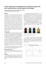
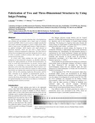
The distorted test images were created by changing their
colours through ICC profiles gamut mapping process. Here, the
absolute colorimetric rendering intent was used with four
standard ICC profiles: Euroscale Uncoated, ISO Uncoated,
PSR Gravure LWC, and Uncoated FOGRA. The gamut of
these ICC profiles and the gamut of sRGB space in ab-plane
are illustrated in Figure 1, where the visualizations have been
obtained from ColorSync Utility included in Mac OS X. As can
be seen from the figure, the ICC profiles can be divided into
two groups based on their dimensions. This was done to ensure
that there would be both larger and smaller differences between
generated distortions.
The selection of images for pilot tests from the candidate
images was done by calculating average CIELAB dE values
and then selecting those image sets that had average colour
difference values on both sides of threshold value. The
threshold value for colour difference discrimination in natural
images is about 2.2 dE ab
/11/. Finally, the selection was further
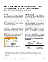
narrowed to eight images. Seven of the images were from the
Photos.com –database /12/ and one was from the CIE TC8-03
test image set /13/. The test images are presented in Figure 2,
where the images are named as Autumn road, Red field,
Mountains, Forest rise, Red brushwood, Park, Table, and
Picnic.
(c)
(d)
(e)
Figure 1. Gamut visualizations of the ICC profiles. (a) Euroscale
Uncoated, (b) Uncoated FOGRA, (c) ISO Uncoated, (d) PSR Gravure
LWC and (e) sRGB.
Autumn road /12/ Red field /12/
Mountains /12/ Forest rise /12/
Red brushwood /12/ Park /12/
Table /12/ Picnic /13/
Figure 2. Selected test images
CGIV 2010 Final Program and Proceedings 511

Test environment
Subjective tests were conducted in a test room with matt
grey painted walls and sealed windows. The viewing conditions
in test room were adjusted to correspond to the sRGB reference
viewing environment, which is presented in Table 1. According
to these parameters the ambient illuminance level of the
viewing conditions was set to approximately 200 lux with
colour temperature of 5000 K. The illumination was done by
using filtered halogen lamps. The illuminance level and the
colour temperature were measured at the beginning of each test
day.
Table 2. sRGB reference viewing environment
Condition
sRGB
Luminance level
80 cd/m2
Illuminant White
x = 0.3127, y = 0.3291 (D65)
Image surround
20% reflectance
Encoding Ambient
Illuminance Level
64 lux
Encoding Ambient White
Point
x = 0.3457, y = 0.3585 (D50)
Encoding Viewing Flare 1.0%
Typical Ambient Illuminance
Level
200 lux
Typical Ambient White Point x = 0.3457, y = 0.3585 (D50)
Typical Viewing Flare 5.0%
Fifteen test participants took part in the test. The age of the
test participants were between 23 to 29 years, and four of them
were female and eleven were men. All test participants had
normal colour vision and all had normal or corrected visual
acuity.
The tests were conducted on a simple image pair
comparison application, which was programmed with Java. The
application includes display for inputting test participant
information, and two displays each presenting one image pair.
The participant information is collected at the beginning of the
test, and after clicking the start button, the two image pair
windows are maximized to fill one display. Before starting the
test, the test participant reads the instructions, including the test
question: which of the two pairs has a bigger difference
compared to other image pair. After these preparations, the test
participant is asked to start the test by clicking the background
of one of the image pair windows. This is expressed by clicking
the pair that has the larger perceived colour difference (see
Figure 3).
Display Two
Figure 3. Example of the pair comparison application: image pairs, one on
each display, are presented to test person, who has been instructed to
select the pair that is perceived to have more colour difference.
The image pairs were presented using Eizo ColorEdge
CG241W displays. The displays were calibrated with Eizo
ColorNavigator Calibration software. The calibration was done
by using a sRGB colour space emulation, which makes it
possible to achieve as close to sRGB colour space full gamut as
possible. The measurements for the calibration were done using
X-Rite EyeOne Pro spectrophotometer. The colour
reproduction performance was worst in bluish hue areas in both
displays, while the average value of CIEDE2000 colour
difference was between 0.4 and 0.6. The displays were also
compared with each other to test their similarity, and even
though the displays were the same model there were clear
differences between them (Table 3).
Table 3. Comparison of the two displays (CIEDE2000)
Average 0.81
Std. Deviation 0.72
Best 90% 0.61
Worst 10% 2.50
Subjective data
The subjective tests, as mentioned, were accomplished
with psychophysical pair comparison tests. Although, the tests
consist of comparison of two image pairs, the factor that is
considered was the difference between two images forming a
pair. Therefore, the law of comparative judgement by
Torgerson /14/ was used in the analysis of the pair comparison
data. The results of the subjective tests are presented in Table 4
and Table 5. Each value in the tables represents the subjective
difference scale value that was calculated from the comparison
judgements. One test participant from total of sixteen
participants, whose judgements differed clearly from other
judgements, was excluded from the data.
Display One
512 ©2010 Society for Imaging Science and Technology

Table 4. Subjective difference scales for image contents
Autumn road, Red fields, Mountains, and Forrest rise, and
ICC profiles: (1) Euroscale Uncoated, (2) ISO Uncoated, (3)
Uncoated FOGRA and (4) PSR Gravure LWC
Mountains
ICC profiles \
images
Autumn
road
Red
Fields
Forrest
rise
(1,2) - (1,3) * 0.201 0.280 0.183 0.580
(1,2) - (1,4) 0.178 0.461 0.318 0.258
(1,2) - (2,3) 0.175 1.223 0.283 0.372
(1,2) - (2,4) 0.059 0.363 0.506 0.087
(1,2) - (3,4) 0.065 0.624 0.383 0.174
(1,3) - (1,4) 0.380 0.181 0.500 0.322
(1,3) - (2,3) 0.377 0.943 0.465 0.208
(1,3) - (2,4) 0.260 0.083 0.688 0.667
(1,3) - (3,4) 0.267 0.344 0.566 0.406
(1,4) - (2,3) 0.003 0.762 0.035 0.113
(1,4) - (2,4) 0.119 0.098 0.188 0.346
(1,4) - (3,4) 0.113 0.163 0.066 0.084
(2,3) - (2,4) 0.117 0.860 0.223 0.459
(2,3) - (3,4) 0.110 0.599 0.100 0.198
(2,4) - (3,4) 0.007 0.261 0.123 0.261
Average 0.162 0.483 0.308 0.302
* Image pair (ICC1,ICC2) compared to Image pair (ICC1,
ICC3)
Table 5. Subjective difference scales for image contents Red
brushwood, Park, Table, and Picnic, and ICC profiles: (1)
Euroscale Uncoated, (2) ISO Uncoated, (3) Uncoated
FOGRA and (4) PSR Gravure LWC
Park Table Picnic
ICC profiles \
images
Red
brushwood
(1,2) - (1,3) * 0.270 0.025 0.680 0.256
(1,2) - (1,4) 0.954 0.444 1.231 0.114
(1,2) - (2,3) 1.095 0.860 1.567 0.062
(1,2) - (2,4) 0.085 0.932 1.478 0.089
(1,2) - (3,4) 0.176 1.027 1.527 0.256
(1,3) - (1,4) 0.684 0.420 0.551 0.142
(1,3) - (2,3) 0.825 0.836 0.887 0.194
(1,3) - (2,4) 0.355 0.908 0.799 0.345
(1,3) - (3,4) 0.094 1.002 0.847 0.000
(1,4) - (2,3) 0.141 0.416 0.336 0.052
(1,4) - (2,4) 1.039 0.488 0.247 0.202
(1,4) - (3,4) 0.778 0.583 0.296 0.142
(2,3) - (2,4) 1.180 0.072 0.088 0.150
(2,3) - (3,4) 0.919 0.167 0.040 0.194
(2,4) - (3,4) 0.261 0.095 0.049 0.344
Average 0.590 0.552 0.708 0.169
* Image pair (ICC1,ICC2) compared to Image pair (ICC1,
ICC3)
The average subjective difference varies significantly between
images. As a high subjective difference means that relatively
many test participants chose that pair as one which has higher
perceived difference, meaning that differences were more
clearly perceived but also that the images have higher colour
differences. The lowest average subjective scale value was for
images “Autumn road” and “Picnic”. The highest average
subjective scale value was for image “Table”. The relationship
between low subjective scale values and high deviation in
judgement of the test participants is evident.
Performance of the metrics
The performance of the computational metrics was
evaluated in relation to the differences of the resulting colour
difference values between two images. Thus, a metric was
capable of predicting perceptual colour difference in complex
images if the difference between two calculated colour
difference values correlated with the subjective difference
(Table 6 and Table 7).
As can be seen from the correlation values in Table 6 and
Table 7, none of the metrics outperform the others in the case
of every image content. The Hue-angle metric had the best
correlation for three of the images with significantly high
performance, while the P-CIELAB metric had also the highest
correlations in three of the image contents, two of them were
with low statistical significance. The iCAM metric was the best
performing metric only for two of the images, but the average
correlation was the highest of the metrics indicating that the
iCAM metric was the best performing metric. The second
highest average correlation was for the Hue-angle metric.
Table 6. Pearson linear correlation coefficients between the
subjective colour differenece and predictions of CIELAB,
CIE94, and CIEDE2000
CIELAB CIE94 CIEDE2000
Autumn road 0.113 -0.279 -0.142
Red field 0.687 -0.070 0.163
Mountains 0.797 0.210 0.647
Forest rise -0.036 -0.061 0.109
Red brushwood 0.361 -0.042 0.077
Park 0.813 -0.045 0.324
Table 0.905 0.688 0.908
Picnic 0.011 -0.249 -0.209
Average 0.457 0.019 0.235
Table 7. Pearson linear correlation coefficients between the
subjective colour differenece and predictions of Hue-Angle,
P-CIELAB, S-CIELAB, and iCAM
Hueangle
P- S- iCAM
CIELAB CIELAB
Autumn road -0.047 0.857 0.273 0.827
Red field 0.742 0.115 0.488 0.798
Mountains 0.878 0.331 0.868 0.563
Forest rise -0.046 0.323 0.195 0.070
Red
brushwood
0.471 -0.301 0.110 0.659
Park 0.832 -0.090 0.637 0.542
Table 0.937 0.839 0.670 0.544
Picnic 0.016 0.132 0.023 0.110
Average 0.473 0.276 0.408 0.514
As it was discussed earlier, the correlation of the metric
varied according to different judgements. If we exclude the two
image contents (Autumn Road, Picnic) that have high variation
in the judgements, the average correlations are rather different.
CGIV 2010 Final Program and Proceedings 513

Now, the iCAM metric has the average correlation of 0.529,
meaning that the metric was only the third best performing
metric, while even the CIELAB metric could outperform it with
average correlation of 0.588. While the best metric in terms of
average correlation is now the Hue-angle metric with average
correlation of 0.636.
The selection between using all eight images and six
images is not straightforward. It might seem proper to use all of
the images in metric performance evaluation; on the other hand,
if test participants could not agree which image pair had greater
difference in excluded images, then it might be proper to
assume that the metrics would not need to predict the degree of
perceptual colour difference that does not exists.
On the other hand, the metrics should be capable of
recognizing image content and related colour difference that is
not perceivable by every observer or is such a colour difference
that has subjective magnitude; for example, distorted image
having colour difference in blue regions compared to an image
having equal difference in red regions. Hence, it would be
needed to study if there are such factors in the image content
that may interfere observer’s conclusion of the colour
difference.
Nevertheless, relatively high performance of the CIELAB
metric with both sets of six and eight images is remarkable.
One reason for the success of the CIELAB metric might be in
the global formation of the colour difference. In such cases, the
effect of structural properties of the image content is minor. For
example, test images “Park” and “Table” have uniformly
located colour differences that were well predicted by the
metric, while the effect of image structure in test images
“Autumn road” and “Red brushwood” may have a greater
effect on the perceived of colour difference which was not
predicted by the CIELAB.
The correlations between metrics evaluated from all
values, are shown in Table 8. As can be seen, the Hue-angle
and CIELAB metrics are significantly correlated with each
other. This is rather remarkable when considering how complex
the process of the Hue-angle metric is, although it is built on
CIELAB. This indicates that the effect of image content is
rather small in the Hue-angle model. The values of CIE94 were
closest to CIEDE2000, while it did not have any correlation
with iCAM metric, and only minor correlation with other
metrics. The CIEDE2000 metric had only minor correlation
with other metrics except CIELAB and CIE94.
Table 8. Correlations between metrics. (1) CIELAB, (2)
CIE94, (3) CIEDE2000, (4) P-CIELAB, (5) Hue-Angle, (6)
iCAM.
2 3 4 5 6 7
1 0,387 0,706 0,004 0,914 0,648 0,786
2 - 0,843 0,330 0,262 0,045 0,272
3 - - 0,301 0,527 0,296 0,536
4 - - - -0,070 -0,103 0,005
5 - - - - 0,603 0,718
6 - - - - - 0,665
Conclusions
Overall, the state of the art metrics that were tested in this
study are not completely capable to predict the degree of
perceived colour difference in images of complex scenes. Two
metrics came up in the comparison: iCAM and Hue-angle. If all
the images are considered, the iCAM is the best performing
metric. While the Hue-angle metric is the best performing
methods if we excluded those image contents that could not be
judged without a high variation in judgements. In this case the
iCAM-metric is only the third best method after CIELABmetric.
Additionally, the iCAM-metric has its strengths in image
appearance modelling, while the Hue-angle metric has its
advantages in modelling the effect of image structure. The
future metric should be a hybrid model that has both image
appearance and image structure modelling capabilities. One
example of a hybrid model could be a metric that uses
segmentation of colour difference map to find spatial areas that
have higher impact on perceived colour difference.
References
[1] Luo. M. R., Cui. G., Rigg. B. The Development of the CIE
2000 Colour- Difference Formula: CIEDE2000. Color Research &
Application. vol. 26. Nro. 5, 340-350 (2001).
[2] Moroney. N., Fairchild. M. D., Hunt. R. W. G., Li. C., Luo.
M. R., Newman T. The CIECAM02 color appearance model.
IS&T/SID 10th Color Imaging Conference, 23-27 (2002).
[3] Zhang. X., Wandell. B. A. A Spatial Extension of CIELAB for
Digital Color Image Reproduction. Proceedings of the SID
Symposiums. 731-734 (1997).
[4] Hong. G., Luo. R. Perceptually based colour difference for
complex images. Proc. SPIE, vol. 4421, 618-621 (2002).
[5] Chou. C-H., Liu. K-C. A Fidelity Metric for Assessing Visual
Quality of Color Images. Proc. 16th International Conference on
Computer Communications and Networks. ICCCN 2007, 1154-
1159 (2007).
[6] Fairchild. M. D., Johnson. G. M. Meet iCAM: A Next-
Generation Color Appearance Model. Proc. IS&T/SID 10th Color
Imaging Conference: Color Science. Systems and Applications, 33-
38 (2002).
[7] Haderberg, J. Y., Bando, E. & Pedersen, M. (2008) Evaluating
colour image difference metrics for gamut-mapped images.
Coloration Technology, vol. 124, Nro 4, 243-253 (2008).
[8] Wang. Z., Bovik. A. C., Sheikh. H. R., Simoncelli. E. P. Image
Quality Assessment: From Error Measurement to Structural
Similarity. IEEE Transactions on Image Processing, vol. 13, Nro 4,
600-612 (2004).
[9] Wang, Z., Bovik, A. C., A universal image quality index,
Signal Processing Letter, Vol. 9, Nro 3, 81-84 (2002).
[10] Witt. K. CIE Color Difference Metrics. In: Schanda. J.
(Edited): Colorimetry: Understanding the CIE System. John Wiley
& Sons. Inc.. Hoboken. New Jersey. 79-100 (2007).
[11] Aldaba, M. A., Linhares, J. M. M., Pinto, P. D., Nascimento,
S. M. C., Amano, K., Foster, D. H. Visual sensitivity to color errors
in images of natural scenes. Visual Neuroscience, vol. 23. 555-559
(2006).
[12] Anon. (n.d) Photos.com (online). Juppiterimages. Updated
13.03.2009 [referred 13.03.2009]. Available in WWW:
[13] CIE (2004). CIE Division 8 – TC8-03: Gamut Mapping.
Guidelines for the Evaluation of Gamut Mapping Algorithms
514 ©2010 Society for Imaging Science and Technology

(online). Updated 02.09.2004 [referred 13.03.2009]. Available in
WWW:
[14] Torgerson. W. S. Multidimensional Scaling: I. Theory and
Method. Pyschometrika. vol 17, Nro 4, 401-419 (1952).
Author Biography
Henri Kivinen received his Master’s degree in Graphic arts
technology from the Aalto University, Finland (2010). This work is his
Master project results at the university. Since then his work at the Aalto
University has included media related research on a broader scope.
CGIV 2010 Final Program and Proceedings 515