Aerodynamic Design of Unmanned and Scaled Supersonic ...

More documents

Recommendations

Info

K. Yoshida and Y. Makino near leading edge. This refinement was performed by removing the load deficit near the leading edge. We used a simple quasi-inverse method for this purpose. This inverse method was formulated by two dimensional supersonic linear theory and applied to wing section every 5% semispan location [3, 11]. The target load distribution was re-calculated to treat the effect of body on warped surface using Middleton and Lundry’s method [12], which was an extension of the Carlson’s method. Furthermore, the chordwise thickness distribution was replaced with the distribution of NACA 66-series airfoil, which was one of laminar airfoils at low speed, because it was found to have also better transition characteristics in supersonic flows [6]. The re-designed configuration was called “2nd Configuration”. (c) Application of natural laminar flow wing design In designing the NLF wing, we originally developed a complete three-dimensional inverse method to achieve the optimum pressure distribution [6]. It consists of both CFD analysis and geometry modification procedure. The governing equation of the modification procedure is based on supersonic lifting surface theory. A panel method was used to solve the equation [9]. Figure 7 shows a flowchart of the inverse design procedure. The target pressure distribution on upper surface was the optimum pressure distribution for the NLF wing. The target pressure distribution on lower surface was estimated by subtracting the optimum load distribution by the Middleton and 1. Target upper Cp C p Transition analysis by e N method 2. Optimum load ΔC p Warp Design by Carlson Method C p 3. Target Cp 4. Inverse Method (NS +Lifting Surface Th.) 5. Designed Geometry final initial Figure 7. NLF Wing Design Procedure Lundry’s method from the target pressure distribution on upper surface. In addition, the “2nd Configuration” was used as an initial configuration. First of all, pressure distribution on the wing surface of the initial configuration was estimated using a JAXA’s CFD solver with turbulent flow condition. Secondly, the pressure difference between the estimated and the optimum pressure distributions was calculated. Thirdly, the increment of geometry was estimated using the pressure difference and the inverse method. Fourthly, the wing section geometries at 14 spanwise stations were modified by adding the increment to the initial configuration. Finally, new wing geometry with fuselage was re-defined by smoothing process using a three-dimensional geometry generation software CATIA. These steps composed one iteration loop. Since we spent most of time for the smoothing process in one iteration loop, it was required about one week for one iteration including CFD analysis. According to the design procedure, we conducted this iteration loop [3, 11]. In each iteration loop, we experienced thicker modification at inboard wing and thinner modification at outboard wing. Such modification was not corresponding to the prescribed spanwise thickness ratio distribution. This meant that our NLF wing design method was not well-posed. Exactly speaking, our target pressure distribution was not satisfied with both warp condition and prescribed spanwise thickness ratio distribution. Although the target pressure distribution should be improved to solve this problem mathematically, it is not easy to find other desirable 8
K. Yoshida and Y. Makino pressure distribution to delay transition satisfying the conditions mentioned above. Therefore, as an approximation, we adjusted the maximum thickness of the modified wing geometry to the prescribed maximum thickness at the smoothing process by CATIA. The “3rd Configuration” was designed after six iterations even though no complete convergence was obtained. However, desirable transition characteristics were not obtained using the SALLY code. The main reason was originated in the resolution of CFD analysis near the leading edge. Therefore, in the re-design phase, the resolution was improved to realize the pressure gradient almost same as that of the target one in accelerated region. Furthermore, we kept the prescribed thickness ratio at outboard wing because of severe structural design requirements. However, we did not adjust the maximum thickness of the modified geometry at inboard wing to approach the convergence. Finally, we selected the modified wing configuration after ten iterations as the “4th Configuration”. Consequently, the “4th Configuration” had the improvement of the pressure gradient near leading edge as we already expected. The transition analysis of the “4th Configuration” by the SALLY code indicated desirable transition characteristics. 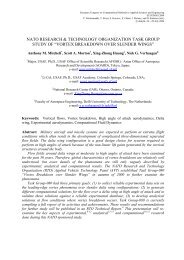The wing section geometry of the “4th Configuration” was shown in Figure 8 and its spanwise thickness ratio distribution was also shown in Figure 5. No adjustment of its maximum thickness to the prescribed one was reflected in thicker distribution at inboard wing region. And this led to a remarkable deviation from the exact supersonic area distribution due to the Sears-Haack body. Naturally, it meant an increase of wave drag due to volume. However, we recognized the validation of the NLF wing concept was more valuable than the validation of high L/D in flight test. The SALLY code is formulated in the framework of incompressible stability theory. Therefore, in the analysis of the supersonic NLF wing, we can not predict transition location quantitatively, including little database for transition criteria on the so-called N value. Furthermore, any codes based on compressible stability theory are not available in Japan. Therefore, at least, to solve the formulation problem, we developed an original compressible e N code, which was called LSTAB code [13]. And we also tried to develop a reliable transition database on the critical N value for onset of transition in supersonic flow. Transition characteristics of the “4th Configuration” were estimated using the LSTAB code as shown in Figures 9. Here we assumed N=14 as the criterion of transition, Y/L 0.0 -0.1 8*z/l 8*(z/L) 0 -0.01 -0.02 -0.03 NEXST-1: NLF Wing 0.3 0.4 0.5 0.6 0.7 x/L x/l Figure 8. Designed NLF Wing Geometry M=2.0, H=15km, N TR. =14 -0.2 α=0.0° α=1.0° α=1.5° -0.3 α=2.0° α=2.5° α=3.0° DP -0.4 Estimated turbulent region HF TC influenced Cp(UPACS: by AS2-grid, the attachmentline LBL(Kaups-Cebeci), contaminationLSTAB(Path B) X/L TBL condition), Preston -0.5 0.0 0.1 0.2 0.3 0.4 0.5 0.6 0.7 0.8 0.9 1.0 Figure 9. Estimated transition locations at H=15km 9
Page 1 and 2: European Congress on Computational
Page 3 and 4: K. Yoshida and Y. Makino completed
Page 5 and 6: K. Yoshida and Y. Makino drag under
Page 7: K. Yoshida and Y. Makino than that
Page 11 and 12: K. Yoshida and Y. Makino generation
Page 13 and 14: K. Yoshida and Y. Makino airplane.
Page 15 and 16: K. Yoshida and Y. Makino configurat
Page 17 and 18: K. Yoshida and Y. Makino minimum pr
Page 19 and 20: K. Yoshida and Y. Makino ACKNOWLEDG

Aerodynamic Design of Unmanned and Scaled Supersonic ...

Create successful ePaper yourself

Delete template?

Save as template?