RESEARCH· ·1970·

. .,
GEOLOGICAL SURVEY
RESEARCH· ·1970·
Chapter.B
GEOLOGICAL SURVEY PROFESSIONAL PAPER 700-B
Scientific notes and summaries of investigations
in geology, hydrology, and related fields
UNITED STATES GOVERNMENT PRINTING OFFICE, WASHINGTON: 1970

UNITED STATES DEPARTMENT OF THE INTERIOR
WALTER J. HICKEL, Secretary
GEOLOGICAL SURVEY
William T. Pecora, Director
For sale by the Superintendent of Documents, U.S. Government Printing Office
·Washington, D.C. 20402 - Price $3.25

CONTENTS
GEOLOGIC STUDIES
Petrology and petrography
Page
Copper in biotite from igneous rocks in southern Arizona as an ore indicator, by T. G. Lovering, J. R. Cooper, Harald
Drewes, and G. C. Cone__________________________________________________________________________________ B 1
Relation of carbon dioxide content of apatite of the Phosphoria Formation to regional facies, by R. A. Gulbrandsen____ 9
Extensive zeolitization associated with hot springs in central Colorado, by W. N. Sharp____________________________ 14
Mafic and ultramafic rocks from a layered pluton at Mount Fairweather, Alaska, by George Plafker and E. M. MacKevett,
Jr-----------------------------------------------------------------------------------------------------
Authigenic kaolinite in sand of the Wilcox Formation, Jackson Purchase region, Kentucky, by J. D. Sims_--- __ --- __ -
21
27
Blueschist and related greenschist facies rocks of the Seward Peninsula, Alaska, by C. L. Sainsbury, R. G. Coleman, and
Reuben Kachadoorian _______________________________________________________.________________ --- _____ -- ___ 33
Structural geology
Allochthonous Paleozoic blocks in the Tertiary San Luis-Upper Arkansas graben, Colorado, by R. E. Van Alstine_____ 43
Geophysics
Calculated in situ bulk densities from subsurface gravity observations and density logs, Nevada Test Site and Hot Creek
Valley, Nyo County, Nev., by D. L. HealeY----------------------------------------------------------------- 52
Geologic and gravity evidence for a buried pluton, Little Belt Mountains, central Montana, by I. J. Witkind, M. D.
Kleinkopf, and W. R. Keefer __________________________________________________ .:. ____________ ---- __ --------- 63
Aeromagnetic and gravity features of the western Franciscan and Salinian basement terranes between Cape San Martin
and San Luis Obispo, Calif., by W. F. Hanna--------------------------------------------------------------- 66
Reconnaissance geophysical studies of the Trinidad quadrangle, south-central Colorado, by M. D. Kleinkopf, D. L.
Peterson, and R. B. Johnson______________________________________________________________________________ 78
Geochronology
Whole-rock Rb-Sr age of the Pikes Peak batholith, Colorado, by C. E. Hedge ______________ - __________ --- __ ------- 86
Distribution of uranium in uranium-series dated fossil shells and bones shown by fission tracks, by B. J. Szabo, J. R.
Dooley, Jr., R. B. Taylor, and J. N. Rosholt---------------------------'------------------------------------- 90
Economic geology
Iron deposits of the Estes Creek area, Lawrence County, S.Dak., by R. W. BayleY-------------------------------- 93
High-calcium limestone deposits in Lanc~ster County, southeastern Pennsylvania, by A. E. Becher and Harold Meisler~- 102
Geology and mineral potential of the Adobe Range, Elko Hills, and adjacent areas, Elko County, Nev., by K. B. Ketner-- 105
Paleontology
Early Permian plants from the Cutler Formation in Monument Valley, Utah, by S. H. Mamay ~nd W. J. Breed_._____ 109
Stratigraphic micropaleontology of the type locality of the White Knob Limestone (Mississippian), Custer County, Idaho,
by Betty Skipp and B. L. Mamet-------------------------------------------------------------------------- 118
Triassic conodonts from Israel, by J. W. Huddle---------------------------------------------------------------
Middle Pleistocene Leporidae from the San Pedro Valley, Ariz., by J. S. Downey ______________________ ------------
124
131
New discoveries of Pleistocene bisons ~nd peccaries in Colorado, by G. E. Lewis _______________________________ ..:___ 137
Stratigraphy
Geology of new occurrences of Pleistocene bisons and peccaries in Colorado, by G. R. Scott and R. M. LindvalL------- 141
Clay mineralogy of selected samples from the middle Miocene formations of southern Maryland, by Karl Stefansson and
J.P. Owens-------------------------------------------~------------------------------------------------- 150
The Gardiners Clay of eastern Long Island, N.Y.-A reexamination, by J. E. Upson_______________________________ 157
III

IV
CONTENTS
Sedimentation
Page
Settling velocity of grains of quartz and other minerals in sea water versus pure water, by C. I. Winegard ____________ B161
Geomorphology
The glaciated shelf off northeastern United States, by R. N. Oldale and Elazar UchupL _ _ _ _ _ _ _ _ _ _ _ _ _ _ _ _ _ _ _ _ _ _ _ _ _ _ _ 167
Analytical methods
Determination of cobalt in geologic materials by solvent extraction and atomic absorption spectrometry, by Wayne
~ountjOY-----------------------------------------------------------------------------------------------
A field method for the determination of cold-extractable nickel in stream sediments and soils, by G. A. Nowlan________
174
177
The fluorimetric method-:-Its use and precision for determination of uranium in the ash of. plants,. by Claude Huffman,
Jr., and L. B. Riley ___________________________ -.__________________________________________________________ 181
Chemical extraction of an organic material from a uranium ore, by~. L. Jacobs, C. G. Warren, and H. C. Granger___ 184
A die for pelletizing samples for X-ray fluorescence analysis, by B. P. FabbL-----------------~-------------------- 187
Ground-water ~echarge
HYDROLOGIC STUDIES
Transmissivity and storage coefficient of aquifers in the Fox Hills Sandst.one and the Hell Creek Formation, ~ercer and
Oliver Counties, N.Dak., by~. G. Croft and E. A. Wesolowski______________________________________________ 190
Preliminary analysis of rate of movement of storm runoff through the zone of aeration beneath a recharge basin on Long ..
Island, N.Y., by G. E. Seaburn ____________________________________________ -----------.,.--- _ _ _ __ _ _ ___ __ _ _ _ _ 196
Ground-water inflow toward Jordan Valley from Utah Valley through valley fill near tl;le Jordan Narrows, Utah, by R. W.
~ower------------------------------------------------------------------------------------------------- 199
Ground-wa.ter contamination
Waterborne styrene in a crystalline bedrock aquifer in the Gales Ferry area, Ledyard, southeastern Connecticut, by
I. G. Grossman----------------------------------------------------~-~------------------------~---------- 203
Surface water
~eandering of the Arkansas River since 1833 near .Bent's Old Fort, Colo., by F. A. Swenson________________________ 210
Trends in runoff, by P. H. Carrigan, Jr., and E. D. Cobb------------------------------------------------------- 214
Relation between. ground water and surface water
Ground water-surface water relation during periods of overland flow, by J. F. Daniel, L. W. Cable, and R. J. WolL- __ 219
The relationship between surface water and ground water. in Ship Creek near Anchorage, Alaska, by J. B. Weeks______ 224
Prairie potholes and the water table, by C. E. Sloan _____________________________!.----------------------------- 227
Erosion and sedimentation
Hydrologic and biotic effects of grazing versus Iiongrazing near Grand Junction, Colo., by G. C. Lusby _______ ------- 232
Sandbar development and movement in an alluvial channel, Rio Grande near Bernardo; N. ~ex., by·J. K. Culbertson
and C. H. Scott--------------~----~-~~----------~----------------~------------------------------------- 237
Geoche·mistry of water
SpectrochemicaJ determination of microgram quantities of germanium in natural water containing high concentrations
of heavy metals, by A. E. Dong ______ _._. ________ .:. _____ . ________________ .:. ____________________ ·-----------'--- 242
Hydrologic techniques
Evaluation of a method for estimating sediment yield, by L~ ~. Shown __ ..,_- ______________________ -_-------------- 245
Dosage requirements for slug injections of Rhodamine BA and WT dyes, by F. A. Kilpatrick ______________ --------- 250
Comparison of a propeller flowmeter with a hot-film anemometer in measuring turbulence in movable-boundary openchannel
flows, by J.P. Bennett and R. S. ~cQuiveY--------------------------------------------------------·· 254
INDEXES
Subject ________._____________________________.__________________._.____________________..,;______ 263
Author------------------------------------------------------------------------------------ 267

GEOLOGICAL SURVEY RESEARCH 1970
Geological Survey Research
1960 __________________________________________________ _
1961---------------------------------------------------
1962 __________________________________________________ _
1963--------------------------------------~------------
1964 __________________________________________________ _
1965---------------------------------------------------
1966 __________________________________________________ _
This collection of 46 short papers is the first published chapter of "Geological Survey
Research 1970." The papers report on scientific and economic results of current· work by members
of the Geologic and Water Resources Divisions of the U.S. Geological Survey.
Chapter A, to be published later in the year, will present a summary of significant results
of work done in fiscal year 1970, together with lists of investigations in prqgress, reports published,
cooperating agencies, and Geological Survey offices.
"Geological Survey Research 1970'~ is the eleventh volume of the annual series Geological
Survey Research. The ten volumes already published are listed below, with their series designations.
1961--------------------------------------------------·-
1968 __________________________________________________ _
1969---------------------------------------------------
Prof. Paper
400
424
450
475
501
525
550
575
600
650
v

GeOLOGICAL SURVEY RESEARCH 1970
COPPER IN BIOTITE FROM IGNEOUS ROCKS IN SOUTHERN ARIZONA
AS AN ORE INDICATOR
By T. G. LOVERING, j. R. COOPER, HARALD DREWES,
and G. C. CONE, Denver, Colo.
;.lb8t?·act.-ln the Sierrita and Santa Rita Mountains of
southern Arizona, rocks from igneous intrusive bodies that are
genetically associated with copper deposits contain as much as
0.03 percent copper; however, biotite separated from these
rocl{S contains as much as 1 percent copper. Rocl{S from igneous
intrusives in the same area that are not associated with copper
deposits contain from a few parts to a few tens of parts per
million of copper, and the biotites separated from them contain
at most 200 ppm copper. The large composite stock on the east
side of the Sierrita Mountains shows a well-defined increase in
the copper content of biotite, from a few parts per million in
the northern part to as much as 1 percent near the copper
deposits at its southern end. Copper anomalies in biotite in the
rocks in this area provide a more sensitive and extensive indication
of associated copper mineralization than do those in the
whole-rock samples.
Biotite has been separated from samples of four
kinds of intrusive rocks, of Precambrian to Paleocene
age, in the Santa Rita and Sierrita Mountains of
southern Arizona. These separates were analyzed spectrographically
to investigate compositional variation
among biotite samples from (1) different intrusives
of similar ages, (2) similar intrusives of different ages,
and ( 3) a single large ore-related stock.
The greatest variation in trace-element content was
found in the copper of these biotites. Copper content
ranges from a few parts per million to 1 percent, and
the highest copper values are in biotite from rocks
that are genetically and spatially related to copper ore
deposits. The ore-related biotites consistently contain
from one. thousand to several thousand parts per million
of copper, in contrast to biotites from "barren" intrusives,
whose coppe1· content is gener.ally only a few
tens of parts per million.
All the biotite samples in which molybdenum was
detected ( ~ 10 ppm) also contain > 500 ppm (parts
per million) copper; however, many of the samples
that contain high copper concentrations show no detectable
molybdenum. None of the other minor elements
in the biotite show any consistent relationship to the
copper content.
The ability of copper to substitute for iron and magnesium
in the biotite lattice and the relatively high
concentration of copper in biotites from quartz monzonite
stocks in Utah and Nevada that are genetically
related to copper ore deposits have been discussed by
Parry and Nackowski (1963, p. 1127, 1137, 1140-1141).
Putman and Burnham ( 1963) also reported sporadic,
but locally high, concentrations of copper in ferromagnesian
mineral concentrates, which consist largely of
primary biotite, from their Boriana Granodiorite in
the Hualapai l\1ountains south at l{ingman, Ariz.
These biotites with high copper content are associated
with minor primary chalcopyrite and come from an
area that shows copper and molybdenum mineralization
(Putman and Burnham, 1963, p. 60, 72, 78-79, 82,
92). However, Bradshaw (1967, p. 143-144) found that
the copper content of biotite from ore-related granitic
rocks in Cornwall and Wales is consistently less than
50 ppm and that it does not differ significantly fr9m
that of biotite from barren granitic intrusives elsewhere
in Great Britain.
The biotite in many of the older intrusives of the
Santa Rita l\1ountains shows strong chloritic alteration.
Copper analyses are reported here only on those
mineral separates that were optically determined to
consist of more than 80 percent biotite ..
Spectrographic copper analyses had previously .been·
made on some whole-rock samples of the same rocks
from which biotite ·separates had been made. The copper
content of ore-associated infrusi ve rocks is higher
than that of barren rocks, but it is more than an order
of magnitude lower than the copper content of the
biotite.
Samples of the freshest rock obtainable were taken
U.S. GEOL. SURVEY PROF. PAPER 700-B, PAGES BI-BS
Bl

B2
PETROLOGY AND PETROGRAPHY
for biotite separates; the biotite is a primary mineral
in all but one of them (a Precambrian granodiorite
from the Santa Rita 1\1ountains which contains secondary
biotite of Paleocene age). Many of the pre-Tertiary
stocks in the Santa Rita Mountains are not represen~ed
in this study because of the intense chloritic
alteration o£ their biotite.
Thirteen biotites were analyzed from the Santa Rita
1\{ountains, and twenty-two from the Sierrita Mountains.
Samples from the Santa Rita 1\1ountains comprise
three. from a large Precambrian stock, two from
an Upper Cretaceous stock, four from small barren
Paleocene stocks, and four from ore-related Paleocene
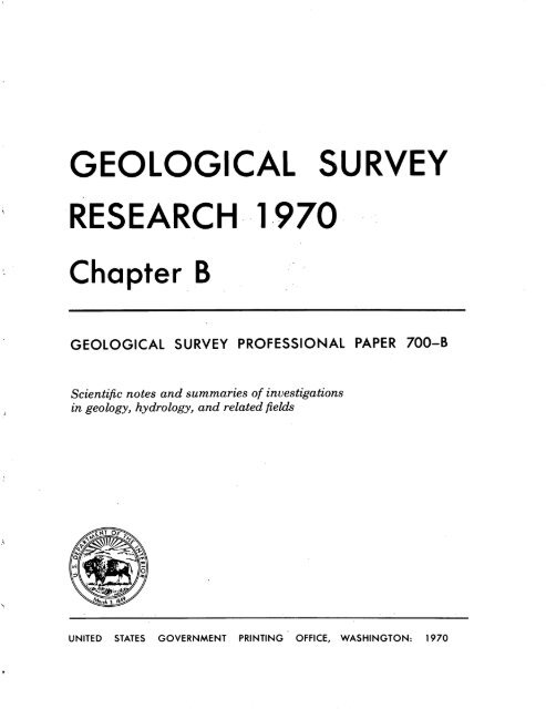
plugs (fig. 1). All the samples from the Sierrita Mountains
were taken from a large composite Paleocene
stock that is related to the Esperanza and Sierrita copper
deposits of the Pima mining district (fig. 2).
GEOLOGIC SE'TTING
The Santa Rita and Sierrita Mountains contain plutonic
and closely related hypabyssal rocks. In the
Santa Rita· 1\1ountains these rocks are of Precambrian,
Triassic, Jurassic, Late Cretaceous, Paleocene, and late
Oligocene ages. In the Sierrita Mountains they are of
Precambrian, Triassic, Jurassic, and Paleocene ages.
The larger stocks in both areas are composite bodies
whose main phases commonly range in composition
from granodiorite to quartz monzonite. The Santa Rita
1\1ountains also are intruded. by numerous small homogeneous
stocks of granodiorite and quartz monzonite
and plugs of quartz latite porphyry. Only the intrusive
bodies from which biotite samples were taken for
this study are shown on figure 1.
The copper deposits of the Helvetia, Rosemont, and
Gr~aterville mining districts i;n the Santa Rita Mountains
are associated with Paleocene quartz latite porphyry
plugs. Those of the Pima mining district in the
Sierrita Mountains are related to Paleocene quartz
monzonite porphyry which occurs as plugs and as a
facies of Paleocene granodiorite stocks.
METHOD. OF MINERAL SE'PARATION AND ANALYSIS
Rock samples were crushed, ground, and sieved. The
60- to 150-mesh fraction· was used for separation and
analysis. The ground s~mple was then placed in bromoform
to float quartz, feldspar, and other light minerals.
The heavy-mineral concentrate from the bromoform,
including the biotite, was washed, dried, and placed
in a n1ethylene iodide solution to float the biotite and
sink all heavy minerals of specific gravity greater than
3.3. The biotite concentrate was again washed and
dried and was then run through a Frantz magnetic
separator at different settings to obtain as pure a biotite
fraction as possible. 1\1ineral impurities other than
chlorite were estimated to constitute less than 5 percent
of this fraction. Chlorite, which cannot be removed
mechanically by this method of mineral separation,
ranged fron1 1 percent to at least 50 percent. All biotite
concentrates were examined optically, and only the
analyses of those in which chlorite was·:less than 20
percent are reported in this paper.
Both whole-rock samples and biotite concentrates
were analyzed by a six-step semiquantitative spectrographic
method which is similar to the three-step
method of l\1yers, Havens, and Dunton ( 1961) . Result~
from the six-step method identify geometric intervals
that have the boundaries 1.2, 0.83, 0.56, 0.38, 0.26, 0.18,
0.12, 0.083, and so forth, and are reported as midpoints
of these intervals by the numbers i, 0.7, 0.5, 0.3, 0.2,
0.15, 0.1, and so forth. The interval identified by the
reported n1idpoint contains the analyst's best estimate
of the concentration present. The precision of a reported
value is approximately plus or minus one interval
at 68-percent confidenc~, or two intervals at 95-
percent confidence.
Petrography
SANTA RITA MOUNTAINS
Rocks sampled in the Santa Rita Mountains include
the Precambrian Continental Granodiorite; the Upper
Cretaceous 1\1adera Canyon Granodiorite; the "barren"
Paleocene stocks of the Helvetia mining district ; and
the ore-associated Paleocene plugs of the Greaterville,
Rosemont, and Helvetia mining districts (fig. 1) .
These rocks, rna pped by Drewes ( 1970a, b), are briefly
described here; more complete descriptions are
planned for future publication.
The Continental Granodiorite forms a large composite
stock in the northern part of the Santa Rita
Mountains. It is exposed in an eastward-tilted structural
block of Precambrian rock that is unconformably
overlain by Paleozoic and Mesozoic sedimentary rocks
and that is intruded by .Paleocene stocks and plugs.
The main phase of the stock is a medium-gray to darkgray
very coarse grained porphyritic biotite granodiorite
that grades to a quartz monzonite. Mafic minerals,
chiefly biotite and chlorite, form a meshwork
pattern around the felsic minerals. Phenocrysts of
light-pinkish-gray microcline or orthoclase as much as
4 em long constitute 5-10 percent of the rock. A mode
of typical Continental Granodiorite contains, to the
nearest percent, quartz, 28 ; plagioclase, 42; orthoclase,
18; biotite, 9; and accessory ilmenitic magnetite, apatite,
sphene, and zircon, 3. This rock is isotopically
dated as Precambrian (Drewes, 1968).

LOVERING, COOPER, DREWES, AND CONE
B3
>-
.....
() I.J.J
...J
...J
Corona de Tucson
EXPLANATION
j !Qun•t' laUte J,.h: (Lre po'Phyry")) ~
~ ~ ~
Granodiorite to quartz monzonite ~
Granodiorite
x2oo
0
H
0::
u
} ~
Granodiorite to quartz monzonite .....
:::E

B4
PETROLOGY AND PETROGRAPHY
has been dated as about 68 m.y. (million years) (P. E.
Damon, written commun., 1964; Drewes, 1968, p. C13).
Six small elliptical stocks of Paleocene age, which
consist largely of light-gray granodiorite, intrude the
structurally complex rocks near Helvetia (Drewes,
1970b). Four of them were sampled for this study (fig.
1). The composition of these stocks is variable, rang- '
ing from granodiorite to quartz monzonite. Their inhomogeneity
is exemplified by a stock in which the biotite
content ranges from 1 to 10 percent. The rocks of
these stocks are distinguishable from the Continental
Granodiorite by their fresher appearance, the absence
of phenocrysts, and the habit of their biotite, which
forms discrete books. J\1odes of these rocks vary
widely; that of the s·ample from the northernniost
stock shown on figure 1, which is fairly representative
of the granodiorite, is, to the nearest percent, quartz,
30; plagioclase, 45; microcline, 13; biotite, 10; and
accessory ilmenitic magnetite, apatite, zircon, and
sphene, 1. The stocks of Helvetia are not associated
with the mineralization of the district. They have been
isotopically dated as about .53 m.y. (Drewes and Finnell,
1968, p. 323; R. F. Marvin, written commun., 1968),
but geologic field relations indicate that they may be
slightly older.
Quartz 1atite porphyry, locally referred to as the
"ore porphyry," forms six small irregular plugs and
many dikes in the Greaterville, Rosemont, and Helvetia
mining districts. The four plugs sampled are
shown on figure 1. The plugs are surrounded by aureoles
of low-grade metamorphosed and mineralized rock.
Copper, lead, zinc, and silver are the principal metals
produced in these districts, but other metals are also
present (Schrader 1915; Creasey and Quick, 1955;
Drewes, 1970c). The porphyry is typically a grayishorange-pink,
closely fracturedrock with a saccharoidal
groundmass. It contains abundant bipyramidal quartz
phenocrysts, sparse small biotite phenocrysts, and
traces of disseminated sulfides. Modes of the porphyry
are very uniform; the ·average of the modes of seven
specimens, to the nearest percent, is quartz, 26 ; plagioclase,
45.; potassium feldspar (largely sanidine), 25;
biotite, 3; and accessory sphene, apatite, magnetite,
zircon, and sulfides, 1. Biotite from three of these plugs
has been isotopically dated as about 56 m.y. (R. F. Marvin,
written commun., 1967).
The quartz latite porphyry appears to have been
emplaced at a higher temperature than that at which
the barren intrusives were emplaced, as indicated by
its bypyramidal quartz and sanidine. The extremely
·irregular shapes of these plugs also suggest that the
parent magma of the plugs was highly fluid, a condition
that would be favored both by high temperature
and by high volatile content. A high metal content of
this magma 'is also indicated by the genetically related
ore deposits.
Biotite concentrates and their copper content
Biotite from the Precambrian Continental Granodiorite
is olive green and contains less than 5 percent
mineral impurities, which .are chiefly chlorite.
Biotite from the Cretaceous Madera Canyon Granodiorite
is 1nodetate brown and contains about 10 percent
ilmenite and sphene as poikilitic inclusions. Approximately
10 percent each of hornblende and chlorite
is present in the mineral concentrates as discrete grains.
Biotite from the Paleocene granodiorite and quartz
monzonite porphyry stocks that have no known copper
deposits associated with them is dark yellowish brown
and contains about · 5 percent hematite, apatite, and
zircon as inclusions. About 5-10 percent chlorite and
minor amounts of sphene and plagioclase are present
as accessory minerals in the concentrates.
Four samples were collected from the quartz latite
porphyry plugs, which are closely related to ·copper
deposits. These plugs are nearly the same age as the
barren monzonite porphyry._ Biotite froin this "ore
porphyry" ranges from light brown to moderate
brown, and contains about 5 percent apatite, rutile, and
ilmenite as inclusions and 5-10 percent chlorite and
sphene as accessory minerals in the concentrate.
Copper concentrations in the biotites of the four
rock types in the Santa Rita Mountains that were
sampled are summarized in table 1. This table illustrates
the marked increase in copper content of biotite
samples from the "ore porphyry" relative to such
samples from both the unmineralized older granodiorite
and the quartz monzonite stocks of approximately
the same age as the mineralized quartz latite porphyry
plugs.
Copper also increases slightly in whole-rock samples
of the ore porphyry, but the copper in biotite separates
TABLE 1.-Copper content of biotite samples from selected igneous
rocks of the Santa Rita Mountains
Rock type
[J. L. Finley, analyst)
Precambrian granodiorite and
quartz monzonite.
Cretaceous granodiorite _________ _
Barren Paleocene quartz
monzonite.
Productive Paleocene quartz
latite porphyry.
Number of
samples
3
2
4
4
Copper content
(ppm)
Range
Mean
30-70 . 50
10Q-200 150
70-150 90
700-7,000 3,400

LOVERING, COOPER, DREWES, AND CONE
B5
TABLI~ 2.-:-Comparison of copper content of whole rock and biotite
m selected samples from the Santa Rita Mountains ·
Rock typo
Precambrian granodiorite _________________ _
Cretaceous granodiorite ___________________ _
Paleocene quartz monzonite _______________ _
Paleocene quartz latito porphyry __________ _
1 J. L. Hurris, nnulyst.
J J. L. ~'inloy, unulyst.
Copper content
(ppm)
Whole Biotite 2
rock'
10
20
10
50
70
200
70
5,000
fr01n these samples shows a far greater increase (table
2). . .
PIMA MINrNG DIS.TRICT, SIER~I.TA
Petrography
MOUNTAINS
All biotite samples from the Pima mining district
can:e f.r01n a ~u.rge composite stock of Paleocene age,
wInch IS genetlcnJly related to the Esperanza and Sierritn,
porphyry copper deposits (fig. 2). This ·stock and
several smaller ones, which are described and shown on
a preliminary ge·oiogic 1nap by Cooper (1960, pl. 1), 1
~re mainly granodiorite. The large granodiorite body
In the western part of the Pima mining district was
named Ruby Sttu Granodiorite for the Ruby Star
Ranch by Livingston, l\1auger, and Damon (1968)
~ 1~111ne which is here formally adopted. The type are~
IS In parts of Tps. 17 and 18 S., Rs. 12 and 13 E. The
granodiorite intrudes intensely deformed rocks of Precambrian
to Late Cretaceous age and is overlain unconforinably
by Quaternary alluvium. The Es~eranza
and Sierrita ore deposits are near the south end of the
large stock, where part of the roof of the stock is exposed.
The c01nposite stock consists of two granodiorite
facies and, near the ore deposits, of several quartz monzonite
facies not distinguished from one another on
figure 2. l\1odal analyses of four specimens from which
the.analyzed biotites were obtained are shown in table
3.
The equigranular, border-phase granodiorite (ta;ble
3, analysis 1) is a light-gray medium-grained rock
which is characterized in hand specimen by recogniz~
able quartz, twinned plagioclase, untwinned potassium
feldspar, equidimensional books of biotite, hornblende,
and small honey -colored crystals of sphene. This rock
1 The "atypical granodiorite" of Cooper (1960, p. 70) shown in the
southwest corner of this prellmlnnry map is now known to be part of
a ~'rllllssic 01· possibly .Turasslc intrusiYe. The granitic rock west of the
San Xavier thrust shown near the north edge of the map, which was
provisionally assigned to the Precambrian by Cooper (1960, p. 68), ls
now believed to be slightly younger than the adjacent stock from whlch
the biotite samples were obtained.
TABLE 3.-M~da~ analyses of roc~s .in and near the Pima mining
d2stnct from wh'tch bwt'ttes were obtained
[Leaders (_ .) indicate not present]
Granodiorite
2 3.
Quartz monzonite
Quartz_ _________________ 25. 1 33. 2 27.4 26. 4
Potassium feldspar and
perthite_______________ 20. 6 19.2 35.4 30.1
Plagioclase______________ 45. 0 42. 8 33. 2 38. 3
Myrmekite_ _____________
Trace
. 3 ----------------
Biotite and chlorite_______ 5. 9 3. 4 2. 8 3. 7
Hornblende______________ 2. 0
~paque minerals_________ . 8 -----.-8------.-8------i.-o
phene__________________ . 4 . 2 -------- . 1
Apatite and zircon________ . 2 . 1 . 2 Trace
Leucoxene, epidote, and
red iron oxide _________________________ _ .2 .4
TotaL______________ 100. 0 100. 0 100. 0 100. 0
1. Equigranular granodiorite, average of three specimens from
eastern border zone of stock. .
2. Porphyritic grano~iorite, average of two specimens from core
of pluton 2.3 mtles northwest of Esperanza mine.
?· Quartz. monzonite porphyry, "ore porphyry," average of three
sp.emmens from two masses 0.5-0. 7 mile north of Esperanza
mme.
4. Aplitic quartz monzonite 0.5 mile north of Esperanza mine.
has gradational contacts with the porphyritic corephase
granodiorite.
The porphyritic core phase (table 3, analysis 2) is
much hke the border phase, but lacks hornblende and
contains from 2 to 10 percent phenocrysts of potassium
fe~dspar wh~c~ are 1(2-3 inches long. It generally contains
less biotite, more quartz, and plagioclase , of a
less calcic composition than the border phase. Two
potassium-argon age dates on the granodiorite facies
are 60 m.y. (Creasey ·and Kistler, 1962) and 59 m.y.
( Dwmon and Mauger, 1966).
The quartz monzonitic part of the stock near the
ore deposits (fig. 2) includes rocks distinguishable
f~om the granodiorite only by their mineral proportiOns,
and als? . finer grained quartz monzo~ite porphyry
a;n.d apht~c quartz monzonite phases. The quartz
monzonite porphyry has sharp intrusive contacts with
the granodiorite at a few places, but gradational contacts
at others. The aplitic quartz monzonite phase was
called biotite-bearing aplite by Anderson and Kupfer
( 1945, p. 5) and is shown as dacite porphyry on a map
by Lynch (1966). It is an intrusive body approximately
1,0?0 feet wide and 1,800 feet long which is
ei?p~aced In quartz monzonite porphyry and granodiOrite.
It crops out half a mile north of the Esperanza
mine, and also forms very small bodies closer to the
mine. The quartz monzonite phases are not separately
distinguished on figure 2.
The quartz monzonite porphyry (table 3, analysis 3)
is light gray to pinkish gray on fresh exposures. Pheno-

B6
PETROLOGY AND PETROGRAPHY.
32 • 00,r.7~~~~~7777~~~~~~~~~~1rll~·~lc.o~·~~~~~-------.------------------------------------------------1_1_11•_o_5_',
EXPLANATION
Paleocene Ruby Star
Granodiorite
grd, gran()(liorite
qm, geneh:c(tlly relnted qu.nrtz '111.011-
zom:te,q
Henvy sUpple, porphyrit1:c rocks
Contact
IXtshed where approX?:m.a.tely loca.ted
1000
X30 X 15000
Sample localities
Showing copper content of b1:otite in
pa.rts per mill1:on
Open-pit mine
Ruby Star
Ranch
£SPERANZA MINE
\:::::::
\:~':::
0 2
3 MILES
FIGURE 2.--Generalized map of composite stock and associated ore deposits in the southwestern part of the Pima mining
district, e·ast orf the Sierrita Mountains, showing sample localities and copper content of biotite.

crysts of white plagioclase, gray quartz, pink potassilPU
feldspar, and biotite make up about half the rock. The
remainder is a fine-grained granular ground-mass of
quartz, potassium feldspar, and a little plagioclase.
Primary accessory minerals include magnetite, apatite,
u.nd zircon.
The aplitic quartz monzonite (table 3, analysis 4) is
u. light-gray nplitic rock whose groundmass consists
ln.rgely of quartz, orthoclase, oligoclase, and biotite in
grains less thnn half a millimeter in diameter. Zoned
oligodase phenocrysts as muc;h •aJS 5 1nn1 long ·rund biotite
books 1-3 mm in diameter are fairly common, and
quartz "eyes" as much as 3 mm in diameter have been
observed but are 1nuch less abundant than in the adjacent
qunrtz monzonite porphyry. The accessory minerals
include magnetite, apatite, zircon, and sphene.
The quartz monzonite porphyry has been dated by
Creasey and· IGstler ( 1962) by the potassium-argon
method n.s 56 m.y. This age 1nay be too young, as the
rock is mineralized in tJhe Esperanza mine, and muscovite
from a muscovite-quartz-sulfide veinlet in this
mine has n potassium-argon age of 61 m.y. (Damon
and l\1auger, 1966)-very nearly the same age as the
granodiorite.
Bi•otite concen,trates and their cop.per conte•nt
The sample localities of the rocks from which the
22 biotite separates were made and the copper contents
of these separates are shown in figure 2. Two copper
values shown for n. single locality represent separate
samples collected tens of feet apart to test the possibility
of sporadic local variation in trace-element
content. ·
The biotite concentrates contain some mineral impurities,
both as discrete grains of foreign minerals
and as poikilitic inclusions of other minerals within the
biotite fiakes. The total content of such impurities in
the various mineral concentrates ranges from less than
5 percent to nearly 20 percent; however, none of the
concentrates contain any ·visible copper minerals.
The five samples from the equigranular border facies
of the granodiorite stock show no consistent features
that di,stinguish them from the 12 samples of porphyritic
granodiorite from the central part of the stock.
I-Iornblende is present as an accessory .mineral in two
of.the five concentrates frmn the border facies· but does
~10t appear in any of those from the porphyritic facies.
Zircon forms inclusions in biotite in 5 of the 12 concentrates
from the porphyritic facies but not in any
of the biotite from the· equigranular facies.
There is a suggestion of a color change in the biotite
of both rock types from north to south in this stock.
Most samples near the southern end of the pluton are'
LOVERING, COOPER, DREWES, AND CONE
B7
1noderate brown to dark brown; those from about a
mile to n.bout 3 miles north of the southern end tend
to be so mew hat lighter brown, and those from localities
more than 3 1niles to the north are olive brown or
1nixed olive brown and shades of light brown.
Biotite from the porphyritic granodiorite contains a
maxin1um of about 5 percent apatite, rutile, ihnenite,
hematite, sphene, and zircon as inclusions. Chlorite,
the most common accessory mineral in the concentrates,
ranges from 0 to about 10 percent of the sample. Minor
amounts of feldspar, hornblende, and sphene are also
present as accessory minerals in a few of the concentrates.
Biotite from the quartz monzonite porphyry and
aplitic quartz monzonite is moderate brown to dark
brown and contains as much as 10 percent of inclusions
of apatite, ilmenite, hematite, rutile, and zircon: Chlorite
constitutes as much as 10 percent of the mineral
concentrate, and minor amounts· of sphene occur in
two of the sam pies. ·
As shown in figure 2, the copper content of the biotites
displays a zonal patterri around the copper deposits.
The highest ·copper concentrations are· in the
biotite nearest the deposits, and anomalous concentrations
extend outward for as much a~ 2112 miles. These
very cupriferous biotites are mostly from quartz monzonite
porphyry and aplitic quartz monzonite, but they
include biotites from both the porphyritic itnd the
equigranular granodiorite. The lithologic diversity of
the samples high in copper content suggests that part
or all of this copper may have been introduced by
hydrothermal solutions at the time of mineralization,
or conceivably could have been introduced by later
circulating ground water. However, coarse hydrothermal
biotite from veinlets in diorite above the Sierrita
ore body' contains only 30 ppm copper. This biotite has
a potassium-argon age of 60 m.y. (S. S. Goldich, written
commun., 1964), the same age as that of the hydrothermal
mica from the ·Esperanza mine.
. · ·Th,e zonal pattern of copper concentration in the
biotite is also shown· by the copper concentration in
whole-rock samples, but it is less impressive (table 4).
The copper content of whole-rock samples from which
biotite was sep~rated for ~his s~udy is given in table 4.
CONCL·US1IONS
The copper content 9f primary bi~tit~ in several rock
types from southe~n Arizona ranges from a f~w parts
.per m!llion t~ 1 percei1t. The concentration of copper
in biotite ·from two differen.t bodies of the same. kind
of rock differs by more than an order of magnitude,
and it varies by three orders of magnitude within a
single large ore-related stock of granodiorite in the

B8
PETROLOGY AND PETROGRAPHY
TABLE 4.-Comparison of copper content of whole rock and
biotite in selected samples from the Pima mining district
Rock type and sample locality
Equigranular granodiorite, 2. 7
miles northeast of Esperanza
mine.
Porphyritic granodiorite, 2.9
miles northwest of Esperanza
mine.
Quartz monzonite porphyry, 0.5
mile northwest of Esperanza
mine.
1 N.M. Conklin, analyst.
2 R. H. Heidel, analyst.
Percentage of
Copper (ppm) copper in whole
rock that is
Wholerock' Biotite 2 concentrated in
biotite
7 5

GE·OLOGICAL SURVEY RESEA·RCH 1970
RELATION OF CARBON DIOXIDE CONTENT OF APATITE OF
THE PHOSPHORIA FORMATION TO REGIONAL FACIES
By R. A. GULBRANDSEN, Menlo Park, Calif.
Abstt·act.-Mnny recent dntn provide n well-defined empirical
relntion between the cnrbonate content and the a-cell dimension
of carbonate fluorapatite, the marine variety of apatite. This
relationship is used ns the basis of an X-ray peak-pair method
for estimating the COn content of apatite. An estimate of the
nverage COn content of npatite in the Permian Phosphoria Formation,
as determined on a representative group of samples by
the peak-pair method, is 1.8 weight percent. Averages for a
series of sections located across major rock facies from southcentral
Idaho to central Wyoming indicate an eastward increase
in the COn content of npatite that possibly was due to an
increase of water temperature.
Carbonate fluorapatite has been recognized as the
compositional variety of apatite in 1narine phosphorites
since Altschuler, Cisney, and Barlow (1952) and
Sil vel'lnan, Fuyat, and Weiser ( 1952) showed that
carbonate was an integral component of the mineral
and that the a-cell dimension, in particular, distinguishes
carbonate fluorapatite from other apatites. The
recent outstanding work of Smith and Lehr ( 1966'),
Lehr, l\1cClellan, Smith, and Frazier (1968), and Mc­
Clellan and Lehr (1969) has now shownthe approxinlate
range of carbonate substitution likely to occur
in apatite and has·established an empirical relation of
this substitution with the mineral's cell dimensions.
These studies of the apatite in a large number of
phosphorites from deposits around the world constitute
a 1nilestone in the mineralogy of 1narine apatite. They
present many compositional, physical, and structural
data, but it is the data on carbonate in apatite that is
of interest· here. It is now possible to determine semiquantitatively
by X-ray measurement the amount of
carbonate in marine apatite. Rather than utilize cell
dimensions, however, a peak-pair method is described
n.nd applied to the apatite in rocks of the Phosphoria
Formation in the '¥'estern United States.
Acknowledg1nent.-The development by Ming Ko,
U.S. Geological Survey, of a computer program to
handle the many and varied· calculations utilized ·here
is greatly appreciated.
CORRELATION OF C0 2 CONTENT WITH THE a-CELL
DIMENSION
It is to be expected that the cell dimensions of a
mineral vary with changes of the mineral's composi~
tion, and McClellan and Lehr ( 1969) show the effect
of compositional changes of apatite upon its cell dimensions.
Although they found that the changes in
the a dimension were correlated best in an expression
treating both carbonate and fluorine, the largest effect
is due to carbonate. A direct correlation· exists therefore
between the carbonate content and the a dimension
of apatite, as shown in figure 1 using the C0 2
content and a-cell unit data of McClellan and Lehr
(1969, p. 1379) for 74 marin~ apatites from deposits in
Africa, Florida, North and South Carolina, and the
Western United States. A least-squares line for the
expression y = a + bx is shown for these data, where
y is C02 percent by weight and x is the a-cell dimen-.
sion in angstroms. Even though the scatter of .. points
is fairly large, the trend is well defined, and the leastsquares
line represents an empirically derived relationship
that is useful for semiquantitative determinations
of the C0 2 content of marine apatites.- A method of
this kind is desirable because the determination is unaffected
by the presence of other carbonate-bearing
minerals as well as other impurities so long as the
X-ray peaks are defined well enough for accurate
merusurement. It doe~s require,' however, rtJhe use of 3Jl
internal standard for an accurate measurement of the
ahsdlute d values, as well as a calcu1ation of tJhe a­
cell dimension. A simpler method for making the C02
determinations is utilized here. It requires only the
measurement of the angular difference between two
X-ray diffraction peaks-the peak-pair method.
U.S. GEOL. SURVEY PROF. PAPER 70G-B, PAGES B9-Bl3
B9

BlO
· PETROLOGY AND PETROGRAPHY
EXPLANATION
1-
z
LoJ
u
a::
LoJ
Cl..
5
1- 4
:I:
e,
i;j
::=
~
..,.:
z
~ 3
z
8
N
8
2
Florida
0
North Carolina and
South Carolina
)(
Africa
0
Western United States
1-
z
LoJ
u
a::
LoJ
Cl..
6
5
1- 4
:I:
e,
i;j
::=
~
..,.:
z
~ 3
z
0
u
N
0
u
2
\
\
\
\
\
\ \
\ \
\ \
\ \
\ \
\ \
\ \
\ \
\ \
\ ~\
\\ \
\ '.
\ ,. .\,
', . . \.
\ \
' .. \
\' :· .\
·~.
'\ ,.
0
\'
\
a , IN ANGSTeOMS ·
FIGURE 1.-Plot of ·co2 weight percent and a-cell dimension of
:niarine apatites. Data from McClellan and Lehr (1969).
Equation of line is v=1014.66-108.25&:, where y=C02
in weight percent, and m=a-cel:l dimension in angstroms.
Standard error of estimate of y=0.5569 (shown by dashed
:lines).
Because the o dimension is much less affected by
carbonate substitution than· the a dimension, peaks
whose indices are of the ( 001) type change less than
other types-(hkl), (hkO); (hOO), or (OkO)-a:ll of
,vhich include a component of the a dimension. A pair
of peaks, one of whiCJh i:s ,an ( 001) type, tJherefore shows
a difference that is proportional to the amount of
carbonate substitution, expressed here as the C0 2 content
in weight percent. The peak· pair method was used
by ·Silverman, Fuyat, and Weiser (1952) to show that
carbonate fluorapatite was different from other apatites.
· The pair of peaks selected here are the ( 410) and the
(004)' which occur around 51.6° and 53.1° 28, respec~
tively, for Cu radiation. They are close together, of
m~dium intensity, and at angles large enough to provide
a useful range of spacing differences, t:..28: A t:..28coo4)-(41'J)
value for each of the 74 samples utilized in figure 1 was
calculated by computer from the cell dimensio11s given
4 2e (o04)-(4 lo)• IN DEGREES
FIGURE 2.-Plot of C02 content and .129- data of apatite
in Phosphoria phosphorites, showing good agreement
with least-squares line calculated with the data of
McClellan and Lehr (1969) (fig. 1). Equation of line is
y=23.6341-14.7361m, where 11=C02 weight percent, and
m=-129-. _Standard error of estimate of y=0.5580
(shown by dashed lines).
by McClellan and Lehr ( 1969) and was used in place of
the a dimension to calculate a new least-squares line.
This line, which now shows the relation of t:..28coo4)-(410)
to C0 2 content, is plotted in figure 2; the standard error
of ·estimate for y ( C0 2 ) in this. new relationship js
0.5580.
The points plot.Jted on figure 2 are d3Jta of apatites in
phosphorites of the Phosphoria FormaJtion that are
independently determined and not. part of those of
McClellan and Lehr (1969) plotted in figure 1. These
new data agree well with those of McClellan and Lehr,
which ·are represented in figure 2 by the least-squares
line and standard-error-of-estimate lines, and add additional
support ro·· the empirical relation. The new data
are from 35 of the 60 phosphorites whose chemical composition
was earlier reported by· Gulbrandsen (1966),
and which do not contain other carbonate-bearing min-

GULBRANDSEN
Bll
erals. The reported C0 2 content of these smnples is
adju,sted here on the basis of their OaO content to
equivalent pure apatite containing a theoretical 55.56
percent CaO. The adjustment is inexact owing to substitu;tions
for calcium but does satisfy the major cor.:.
rection needed for !the variable amounts of impurities
present in the rock sa1nples. The ~28 measure ..
ments were made. on chart recordings of % 0
rpm
traverses througfu ~the angular range required to record
the pealr pair using a Norelco X-ray diffractometer
with Cu radiation.
Another pair of peaks ·that can be used for the measurement
as just described is made up of lthe two major
peaks whose indices are ( 002) and ( 300) and that occur
with Cu radiation around 25.9° and 33.1° 28, respectively.
Because resolution decreases with decreasing 28,
owing to the nature of the sine function, this p~ir of
peaks is not as good as the (004) and ( 410) pa1r for
the measurement of C02 content. The ( 002) ·and ( 300)
pair is of value, however, because both peaks ~e o:f
strong intensity and can be used for C02 estimates
where rbhe (004) and (410) pair of peaks is too weak or
too poorly defined to be measured. The least-squares
line for this peak-pair relationship is not plotted here,
but the equation for the line is
where
y= 185.0+ 25.5740w
y=C02 weight percent and
ro=~28° -·
The standard error of estimate is 0.5295. The data used
for this calculation are again those of McClellan and
Lehr (1969).
Because the 60 phosphorites of Gulbrandsen ( 1966)
make up the best available representation of phosphorites
of the Phosphoria Formation, the ~28-
measurements for these samples are listed in table 1
along with the C02 determinations made from the relationship
represented by the least-squares lines of figure
2. The C0 2 values shown in parentheseJS in the taJble
rure tJhose adjusted fron1 che:mioal·runalyses ·and used in
figure 2. The average C0 2 content of the 60 S'amples,
1.8 weight pel'Cent, provides an estimate of the 'average
C0 2 content of apatite in the Phosphoria Formation,
It is m·M·kedly low in comparison with the m·ain mass of
values shown in figure 1·for apU~titein some of the major
phosphate deposits of the world. This indicates a difference
in oplthnum conditions for apatite deposition
between those in the Phosphoria and those in other deposits.
A possible explanation for this difference is revealed
by run ex·amination of the relation of the C02
content of Phosphoria apatite to regional facies.
RELATION OF C0 2 CONTENT OF APATITE
TO REGIONAL FACIES
The Permian rocks of southern Idaho and Wyoming
exl~ibit west-to-east facies changes that McKelvey, Williams,
Sheldon, Cressman, Cheney, and Swanson (1959,
p. 2-5) consider to represent environmental changes
due to an eastward shallowing and warming of sea
water. From south-central Idaho to central Wyoming,
the dominant li·thologies change from chert, mudstone,
and phosphorite to carbonate rock. The region of
greatest phosphrute deposition is in southeastern Idaho
near the Wyoming border.
The C02 content of apatite in 368 samples of phos.:.
phorites and phosphatic rocks (generally containing
more than 10 percent P 20 5 ) from nine sections locwted
along the west-east facies change has been measured by
the X-ray method thrut utilizes the ~28 relation
shown in figure 2. These data are summarized in table 2.
Figure 3 shows the locR!tion and the average C02 content
of apatite in each seotion. ·
In the region where the greatest amount of phosphate
was deposited, represented by sections 2, 3, and
4 (Trail Canyon, Mabie Canyon, and Montpelier Canyon),
the average amount of C02 in the apatite is 1.7
to 1.8 weight percent, an amount practically the same
as the 1.8 weight percent estimated above for the
Phosphoria Formation as a whole. Marked changes are
evident, however, to both the west and east of this
region; the C02 content is lower to the west and about
twice as great to the east in central Wyoming. The
greatest contrast is between the westernmost and easternmost
sections, and it is emphasized by the range of
values in the sections presented in table. 2. The Mud
Spring section, locality 1, and the Conant Cre~k section,
locality 9, do not overlap in their ranges of C02
content, but both overlap with most in-between sections.
The extremes are especially interesting, because the
dominant lithologies or facies of the two regions are
also distinctly different. At Mud Spring, locality 1, the
principal lithologies are chert, mudstone, and phosphorite.
There are no carbonate rocks present, and no
carbonate minerals have been detected by X-ray analysis.
In contrast, the Conant Creek section, locality
9, is composed predominantly of carbonate rock, but
also contains chert, mudstone, siltstone, sandstone, and
phosphorite. Some of the rocks at Conant Creek are
glauconitic and some contain appreciable gypsum. se.ctions
7 and 8 are similar to Conant· Creek in th~ir ma1n
.features. The western sections, intermediate in C02
content, are also intermediate in the lithologies represented.
372-490 0 - 70 - 2

B12
PETROLOGY AND PETROGRAPHY
TABLE l.-C02 determinations by X-ray diffraction measurements, ~20coo4)-C4to>, of apatite in phosphorites of the Phosphoria Formation
[Samples are those chemically analyzed (Gulbrandsen, 1966, table 1)]
Measurement No.I
..1.29(004)-(410)
(degrees)
C02 (weight percent)
X-ray
Cbemical2
Meastirement No.I
A29

GULBRANDSEN
B13
cance of the variable composition of marine apatite
and the differences among environments in which the
phosphate deposits of different ages and in different
pnrts of the world were formed.
REFE.RENCES
Altschuler, z. S., Cisney, E. A., and Barlow, I. S., 1952, X-ray
evidence of the nature of carbonate-apatite [nbs.] : Geol.
Soc. America Bull., v. 63, no. 12, pt. 2, p. 1230-1231.
GuliJrnudsen, R. A., 1960, Petrology of the Meade Peak phosphatic
shale member of the Phosphoria Formation at Coal
Cauyou, 'Vyoming: U.S. Geol. Survey Bull. 1111-C, p. 71-
146.
--- 1966, Chemical composition of phosphorites of the Phosphoria
ll"ormution: Geochim. et Cosmochim. Acta, v. 30,
p, 769-778.
J.Jehr, ;r. R., McClellan, G. H., Smith, J. P., and Frazier, A. W.,
1!)68, Characterization of apatites in commercial phosphate
rocks, in Phosphates naturals-Phosphates dans !'agriculture:
Colloque internntionul sur les phosphates mineraux
solides, 'l'oulouse 16-20 Mui 1967, v. 2, p. 29-44.
McClellnn, G. H., nnd Lehr, J. R., 1969, Crystal-chemicnl investigution
of natural apatites: Am. Mineralogist, v. 54, nos.
9-10, p. 1374-1391.
McKelvey, V. E., Armstrong, F. C., Gulbrandsen, R. A., and
Campbell, R. 1\:L, 1953, Stratigraphic sections of the Phosphoria
formation in Idaho, 1947-48: U.S. Geol. Survey Circ.
301, pt. 2, 58 p.
McKelvey, V. E., Davidson, D. F., O'Malley, F. W., and Smith,
L. E., 1953, Stratigraphic sections of the Phosphoria formation
in Idaho, 1947-48: U.S. Geol. Survey Circ. 208, pt. 1,
49 p.
McKelvey, V. E., 'Villiams, J. S., Sheldon, R. P., Cressman, E. R.,
Cheney, T. M., and Swanson, R. W., 1959, The Phosphoria,
Park City, and Shedhorn formations in the western phosphate
fleld: U.S. Geol. Survey Prof. Paper 313-A, p. 1-47.
Sheldon, R. P., 1963, Physical stratigraphy and mineral resources
of Permian rocks in western Wyoming: U.S. Geol.
Survey Prof. Paper 313-B, p. 49-273.
Silverman, S. R., Fuyat, R. K., and 'Yeiser, J. D., 1952, Quantitative
determination of calcite associated with carbonatebearing
apatites: Am. Mineralogist, v. 37, nos. 3-4, p. 211-
222.
Smart, R. A., 'Varing, R. G., Cheney, T. M., and Sheldon, R. P.,
1954, Stratigraphic sections o_f the Phosphorif!. formation in.
Idaho, 1950-51: U.S. Geol. Survey Circ. 327, 22 p.
Smith, J. P., and Lehr, J. R., 1966, An X-ray investigation of
carbonate apatites: Jour. Agr. and Food Chemistry, v. 14,
no. 4, p. 342-349.

GE,OLOGICAL SURVEY RESEA·RCH 1970
EXTENSIVE ZEOLITIZATION ASSOCIATED WITH HOT SPRINGS
IN CENTRAL COLORADO
By WILLIAM N. SHARP, Denver, Colo.
Abstract.-Extensive zeolitization that accompanied formation
Qf laumontite-leonhardite in shattered quartz monzonite at the
base of Mount Princeton in central Colorado is attributed to
hot silica- and calcium-bearing alkaline waters reacting with
the country rock at depth. The shattered and altered rocks and
active thermal springs are related to faults that are part of the
upper Arkansas Valley structure system. Apparent zoning of
mineral assemblages around the thermal centers seems similar
to that in other thermal areas, and is significant in terms of
depth of formation, temperature, and pressure.
Two masses of shattered quartz monzonite are exposed
as conspicuous white, chalky bluffs along Chalk
and Cottonwood Creeks at the base of Mount Princeton
in Chaffee County, Colo. These bluffs are outstanding
mostly because of their color, which is largely a
result of abundant leonhardite, a calcium zeolite. Hot
springs issue from the base of the cliffs in both creek
valleys; the Mount Princeton Hot Springs occur at
Chalk Cliffs on Chalk Creek, and the smaller Cottonwood
Hot Spring occurs along Cottonwood Creek.
The purpose of this paper is to briefly describe these
occurrences of zeolitized rocks, and to give some suggestions
as to their possible geologic significance.
Chalk Cliffs at Mount Princeton Hot Springs has
been a landmark in central Colorado for many years.
The white, rubbly, steep bluffs rise several hundred
feet above the hot springs along Chalk Creek, and
form the north wall at the entrance of Chalk Creek
canyon, which is along the west side of the Arkansas
Valley (fig. 1). ~1ount Princeton, with an altitude of
14,197 feet, towers over these cliffs, which have been
well lmown from the time of legendary Indian visits
before white settlement, through the mining and railroad
operations in 1880's, the grand hotel-spas in
1920's, to the present era of modern swimming pools
and commercial greenhouses. Indians allegedly used
caves formed in the cliffs as steam baths and healing
sites. This bit of folklore does not seem to be borne out
by the nature of the caves, which are not spring sites;
nevertheless, the place has been an attraction for many
years. Hortense Hot Spring, one of the l\1ount Princeton
Hot Springs group, is the hottest spring (83°C) in
the State. Its output is used largely as a heat sour('P
in greenhouses and mountain homes.
Cottonwood Hot Spring, on Cottonwood Creek, a.
few miles to the northwest of Chalk Cliffs near thE'
mouth of the narrow creek valley, marks a smaller
thermal area than that of the Mount Princeton Hot
Springs, but is similarly situated at the edge of a large ·
zeolitized mass exposed for several miles along Cottonwood
Creek. The cliff walls of the valley are considerably
less spectacular than Chalk Cliffs, and are generally
less zeolitized.
GEOLOGIC SETTING
The regional geology is generalized in figure 1. The
structural framework of the upper Arkansas Valley is
only partly understood. The elements shown were compiled
from field studies and photographic interpretation
by the author,- from recent mapping by Van Alstine
( 1966) and Brock and Barker ( 1966), and from
unpublished gravity work of J. E. Case, all of the U.S.
Geological Survey.
The upper Arkansas Valley north of Salida is a narrow,
north-trending, downdropped trough bounded by
a complex of mostly normal, steeply dipping faults.
This structural valley is accentuated by a rugged
mountain system on the west and rugged but less conspicuous
highlands on the east. The east side of the
trough is marked generally by a single, narrow fault
zone. The boundary faults on the west side appear to
be more complex, and the total downward displacement
is accumulated along several faults both paralleling
and transecting the valley.
The sedin1ents in the Arkansas Valley are river deposits
of the Dry lT nion Formation of Miocene and
B14
U.S. GEOL. SURVEY PROF. PAPER 70G-B, PAGES Bl4-B20

SHARP
B15
106"15'
EXPLANATION
Valley fill materials
Holocene terrace gravels and Pleistocene
glacial outwash overlying
Pliocene and Miocene Dry Union
Formation. Generally marks
extent of Ar·kansas Valley
Tertiary Mount Princeton
Quartz Monzonite
Generalized outline shown
D
Other rocks
Tertiary quartz rnonzonite and
granite, Paleozoic sedimentary
r·ocks, and Precambrian gneisses
Contact, approximately located
Faults
Das hed w here not clearly evident;
dotted w here covered. Accentuated
along boundary of "wedge"
.:§.:;
GtJ}irNISON
ii
Zone of zeolitized shattered
quartz monzonite
Queried where extent not known
•
Spring
X'
Mine
0
5 10 MILES
Strike and dip of shear plane
FIGURE 1.- Part of tble upper Arkansas Valley, showing st:Tuctural featuTes, hot springs, and zeolitized zones.
Pliocene age that are overlain by glacial outwash and
moraines of Quaternary age (Tweto, 1961). The
trough, therefore, probably formed largely in mid­
Tertiary time.
The mountains east of the Arkansas Valley are composed
predominantly of Precambrian granitic gneisses,
overlain in places by upper Tertiary flows and pyroclastic
rocks of rhyolitic to andesitic composition. The
Sawatch Range west of the Arkansas Valley consists
chiefly of Precambrian batholiths of quartz diorite
and granodiorite, and the lower Tertiary batholith of
Mount Princeton Quartz Monzonite.
A structural element of special significance to this
study is the northwest-trending fault zone that crosses
the valley diagonally from near Salida to the Mount
Princeton area, where it merges with faults that form
the west boundary of the valley northward to the
Mount Harvard area (fig. 1). The southern part of
this fault zone contains the commercial fluorite deposits
at Browns Canyon and also gives rise to warm
springs containing more than normal amounts of
fluorine (Russell, 1945). Farther to the northwest, in
the same fault zone on the west side of the valley,
water of the Mount Princeton and Cottonwood Hot

B16
PETROLOGY AND PETROGRAPHY
Springs also contains anomalously large amounts of
fluorine. The fault zone, marked by these two hot
spring areas, appears to be the east edge of a northpointing
wedge of greatly sheared and shattered rocks,
mostly Mount Princeton Quartz ~fonzonite. The wedge
is bounded on the west by a less clearly defined shear
zone extending from Mount Shavano on the south to
Mount Yale and possibly ~fount Harvard on the north
at a point of the wedge. The shattered rocks of this
faulted wedge have been zeolitized in the vicinity of
Mount Princeton.
ZE,OLITIZED ZONES ~NO STRUCTUR-AL CONTROL
The large bodies of zeolitized quartz monzonite are
exposed best in the canyons of Chalk and Cottonwood
Creeks that transect the faultbound wedge (fig. 1).
Chalk Cliffs is the most conspicuous outcrop of
zeolitized rocks, and leonhardite is abundant in these
rocks for a distance of more than a mile along the
cliffs. Chalky white leonhardite fills cracks and coats
rock fragments in the highly shattered and sheared
quartz monzonite to such degree that it imparts a
bright white hue to the normally gray host rock. Besides
being noticeably white, the zeolitized cliffs are
extremely rugged and contain many steep blind canyons.
Several shallow, wide-mouth caverns dot the
walls of the cliffs and terminate some of the short steep
canyons. These caverns characteristically have flat
backs and steeply inclined floors and appear to have
formed mostly by spalling of fragmental material
from beneath flat faults. There is no evidence that
these features are solution cavities or sites of recent hot
springs.
Chalk Cliffs seems to represent in part a locus of
intense alteration and metasomatism. Hortense Hot
Spring of the Mount Princeton Hot Springs group
near the east end of the cliffs is surrounded by several
hundred feet of greenish-gray propylitized fault gouge
and brecciated quartz m.onzonite-a zone that grades
outward abruptly into the zeolitized rocks of the cliffs.
This zonation probably is significant in accounting for
the zeolite bodies. The propylitiz~d material, which is
marbled with greenish-gray and white veins, consists
largely of a mixture of chlorite, quartz, illite, and
epidote with minor amounts of calcite and fluorite.
White vein material is mostly calcite with subordinate
amounts of quartz and fluorite.
Much of the char:acter of Chalk Cliffs just described
and the extent of the cliffs seem due to the intersection
here of at least three faults or fault zones. The principal
fault, which passes through the east end of the
cliffs, extends northwest beyond the Mount Princeton
Hot Springs and through the Cottonwood Hot Spring
site, and feathers out near Mount Harvard. Joining
this fault at Chalk Cliffs is a rather wide zone of faults
that extends south to southwest from Mount Princeton
Hot Springs along the. west edge of the Arkansas
Valley. North-striking, west-dipping shear planes in
this fault zone are conspicuous in the cliffs west of the
springs.
An additional shear zone, oriented N. 60° to 70° W.,
transects the major fault associated with the hot
springs at Mount Princeton. This zone is the least
extensive and is not traceable outside the area of
known zeolitized rocks and hot springs ; however, this
group of shear planes appears to control the distribution
of hot springs for about three-fourths of a mile
along the creek at the southeast base of Mount Princeton.
Zeolitized rocks similar to Chalk Cliffs extend along
Cottonwood Creek, west of Buena Vista, from the easternmost
exposures of crystalline rocks at the mountain
front near the hot spring, almost continuously for
about 4 miles westward in the valley of South Cottonwood
Creek. The zone is near the north end of the
structural wedge and extends almost the entire width
of the wedge. The zone also is marked by very rugged
cliffs particularly along the northwest side of the
valley; but, except for the strongly zeolitized fault
zone directly above Cottonwood Hot Spring, these
cliffs are not as conspicuously mineralized as Chalk
Cliffs.. , ·
In the zeolitized crystalline rocks along Cottonwood
Creek, faults· and zones of shearing trend predominantly
north to northwest. The prevailing direction of
the numerous shear planes near the hot springs is N.
30° W. toN. 10° W. Farther west along the valley, the
south-facing slopes of the mountain mass between the
South Cottonwood and Middle Cottonwood Creeks are
extremely broken and eroded to a rugged topography.
~fuch of this ruggedness is due to several north-trending
faults transected by fractures oriented N. 40° W.
to N. 80° E. White fracture fillings of leonhardite and
calcite are obvious in the cliffs for a distance of several
hundred feet above the valley. Probably some of these
structural "features extend southward across South
Cottonwood Creek and through the Mount Princeton
mass to connect with structures in the Chalk Creek
drainage.
Good exposures of fault zones and zeolitized rock
also can be seen along a steep vehicle track on the east
face of ~fount Princeton, about a mile north of Chalk
Cliffs. North-trending fault planes and zones in shattered
quartz monzonite are filled with leonhardite to
such a degree that it seems reasonable to suspect that
sparsely zeolitized rocks extend much farther north-

~b _______________
ward frmn Chalk Cliffs along the mountain front than
indicated on figure 1, ttnd could be virtually· continuous
with the zeolitized cliffs in the eastern part of the
Cotton wood Creek canyon.
The zones of zeolitization along both Cottonwood
Creek and Chalk Creek appear to extend 1,000-2,000
feet above the valley floor, but the exact nature of the
rocks high on the valley walls and on l\1ount Princeton
has not been determined.
The l\1ount Princeton Quartz l\1onzonite involved in
this extensive crushing, thermal alteration, and zeolitization
is gray, medium-grained, biotitic quartz monzonite.
Locally the rock is porphyritic; phenocrysts of
pink !(-feldspar are conspicuous in an even-textured,
medium-gntined groundmass containing much lightgray
plagioclase. The quartz monzonite, in all size
frngments down to sand -sized material in most of the
faults 11nd shattered rocks, is only slightly altered.
Biotite is generally converted to chlorite, but feldspars
ttre ttppttrently little changed. Both plagioclase and K­
feldspni.· nre ttt most only clouded; albitization which
commonly aocompatnies formation of Ca-zeolites is not
evident.
ZEOLITE
Leonhardite :is virtunlly the only zeolite found in tlie
area, and it ranges in appearance from white and yellowish-white
pulverulent coatings on weathered surfaces to
white tuld pink, sparkling, mrutted crystals in newly
broken rocks. The material that fills fractures encloses
rock 'chips n.nd sand-sized grains of n1ost minerals of
the host .rock. The individualleonhardite crystals rarely
are more than 1 mm long and 0.2-0.3 1run across. The
indices of refraction are about 1.50a and 1.51y, and
Ineasurements of extinction angles in the prism zone
rnnge from about 40° to 65° with a noticeable change
in chnracter from length fast to length slow at about
44°. This chnnge is characteristic of leonhardite and denotes
orientation from 010 to 110 position in the prism
fragments ( Coom.bs, 1952, p. 812).
X-rny diffraction patterns of air-dried material from
throughout the zeolitized zones match closely the data
for leonhardite published hy Coombs (1952) and Laphatn
(1963). Some minor shifts in reflections are general
from sample to sample and a conspicuous reflection is
found at 9.5-9.4 A. This reflection was not reported by
Coombs, but it was noted by Lapham ( 1963).
Leonhardite forms by a slight dehydration of laumontite
( Cao.nAl Si20o · 21-120), and the dehydration process
is rendily reversible (Coombs, 1952). It seems reasonable
to presume that leonhardite in the exposures in this
area grades to dominantly laumontite below the surface.
In leonhardite frmn Chalk Cliffs the potassimn
content is anomalously high (table 1).
.SHARP
B17
TABLE !.-Semiquantitative spectrographic analysis of leonhardite
from Chalk Cliffs
[Analyst, Barbara Tobin. M, major constituent, >10 percent]
Si ______·__________ _
Al ________________ Fe _______________ _
~g _______________ _
Ca ~-----------~
~a _______________ _
]{________________ _
Ti ________________ _
~n _______________ _
Ba _______________ _
Be _______________ _
Ce--------------~-
~
~
0. 7
.5
~.
.7
1.'5
. 07
. 03
. 02
. 0005

B18
PETROLOGY AND PETROGRAPHY
TABLE 2.-Chemical analyses of water from Chalk Creek and hot
springs at Mount Princeton, Cottonwood Creek, Poncha Hot
Springs, and Browns Canyon, Chaffee County, Colo., and
spectrographic analyses of residues
fChemical analyses 1-3, by M. J. Fishman and C. G. Angelo; 4, by H. C. Whitehead;
and 5, by C. R. Howard. Spectrographic analyses, by P. R. Barnett. Leaders( __ )
indicate not determined]
1 2 3 4 5
Hortense Cottonwood Chalk Poncha Spring at
Hot Spring, Hot Spring, Creek, Hot u.s.
Mount Cottonwood Mount Springs, Fluorspar
Princeton Creek Princeton main mine,
springs Browns
Canyon
Temperature, °F
(~C). _________ 183 (83.8) 126 (52.2) 52 (11) 158 (70) 67 (19.4)
pH _______________
8.9 8.9 7. 5 7. 6 ------------
Chemical analyses (parts per million)
. Si02--------- 72 52 7. 8. 84 38
AL-~------- Fe __________
. 40 . 08 . 05 . 53 --------
.11 0
Mn _________
0 . 46 . 04
0 0 . 02
Ca __________
. 10 --------
3.4 6. 3 14 17 7. 9
Mg- - - - - - - - - 0 .3 1 .2 1.8
Na __________
K ___________ 94 98 2 190 151
2. 9 2. 5 .8 6. 6 4. 8
HCOa------- 44 55 33 210 127
CO a- ________ 19 9 0 0 4. 9
804-------.;.- 101 98 19 200 142
CL ___ ._ _____ 9. 5 26 .4 54 53
F ____ . _______ 13 13 .4 11 13
NOa---- __ -.- _ 2 .4 .4 0 0
P04-------·-- 0 0 0 . 02 --------
Dissolved
solids:
Calculated
1 _____
339 332 62 667 474
ROE 2 _____
334 344 70 ----------------
AL ________ _
Ba _________ _
Be _____ . ____ _
B __________ _
Or_ _ _ _ _ _ _ _ _ _ ·
Co _________ _
Cu _________ _
Fe _________ _
Pb _________ _
LL ________ _
Mn ________ _
Mo ________ _
NL ________ _
Ru _________ _
Ag_---------
Sr _________ _
Sn _________ _
TL ________ -
v __________ _
Zn _________ _
Zr _________ _
Ga _________ _
Spectrographic analyses (values in llg/1)3
-87.
10

teration probably depends greatly on the relative
chemical activities of the I-120 and C02 in the system.
At high activities of If 2 0 relative to C0 2 , and other
factors being favorable, the zeolite facies forms. These
conditions generally prevail in thermal areas where hot
water has a. pH of 8 to 9, a feature pointed out by
'¥hite and Sigvaldason ( 1963) ; C0 2 is maintained as
bicarbonate, and its activity relative to H 2 0 is kept
low. Reversing the relative values of the chemical
potentials fn.vors formation of calcite and the claybearing
(kaolinite-pyrophy llite) assemblage.
'¥hite and Sigvaldason ( 1963) emphasized also the
significance of epidote in mineral assemblages in hotspring
systems as an indication of conditions of formation.
In relating the depth and corresponding temperature
to formation of epidote in hot-spring systems,
they concluded that if epidote occurs as a hydrothermal
product in exposed rocks, erosion of at least
1,300 feet ( 390 m) of cover is indicated.
In this framework, it seems likely, therefore, that
the less-hydrated zeolite near 1\fount Princeton was
formed, while still deeply buried, by the metasomatic
action of hot mineral water on fine-grained debris in
t.he large masses of shattered quartz monzonite. The
rock grains and flour, between fragments and in shear
zones, may have supplied some of the materials for
laumontite, but the generally unaltered condition of
the rock fragments strongly suggests that most materials
were supplied by ascending hot water. The
abundant calcium in the zeolitized zones, in both leonhardite
and calcite, seems to be the principal material
added to the system, either from a magmatic source or
from deeper and more extensively altered and leached
quartz monzonite. The lack of albite (or adularia) associated
with the zeolite zones argues against a simple
in-place lenching process for the supply of components.
I-In.y ( 1966, p. 105) stnted more strongly, after Turner
(in Fyfe n.nd others, 1958), thnt interdependent ren.ctions
like this n.re sensible in zones of zeolite faciescomponents
released in tt renction at one place supply
mn.teriu.ls for minerttls like lnumontite at another.
At 1\fount Princeton the temperature during zeolitization
wns without doubt in excess of the present temperature
of issuing wn.ter (mttximum 83°C). Maximum
tempern.ture would depend in part on ·'the depth of
zeolitizntion, which cttn only be estimnted. If late
middle Tertiary time was the time of zeolitization, the
depth might be roughly the distnnce between the creek
level nnd the top of 1\fount Princeton, approximntely
1,800 m (5,900 ft), which is the amount of erosion that
hn.s occurred since uplift in lnte middle Tertiary time.
If liberal latitude is permitted in the estimate, the
,SHARP
BI9
depth of formation probably was nt least several hundred
n1eters. These environmental conditions easily fit
within the rnnges of temperatures (145°C to 220°C)
and depth (150 m to 2,000 m) for formation of laumontite
existJing rut W airakei, New Zealand, ·and in Iceland.
At ·l\fount Princeton a "laumontite (leonhardite)
stage" and a highly propylitized aureole (chloriteepidote-clay
assemblage) around Hortense Hot Spring
are known. Perhaps other zeolite mineral assemblages
are not present, but the known association, viewed in
the framework of the facies concept, invites speculation
that tt more complex sequence of mineralogical
changes extends to deeper levels. Additional study of
these zeolitized zones could provide more details concerning
the geologic development of the Chalk Cliffs
and Cottonwood Creek zeolitized zones themselves and
their possible downward change into other mineral
assemblages, and also expand the understanding of the
geologic evolution of the Arkansas Valley.
Drock, M. R., and Barker, Fred, 1966, Geologic map of the
Mount Harvard quadrangle, Gunnison and Chaffee Counties,
Colorado: U.S. Geol. Survey open-file report.
Coombs, D. S., 1952, Cell size, optical properties and chemical
composition of laumontite and leonhardite, with a note on
regional occurrences in New Zealand: Am. Mineralogist,
v. 37, nos. 9-10, p. 812-830.
-- 1960, Lower grade mineral facies in New Zealand: Internat.
Geol. Cong., 21st, Copenhagen 1960, Rept., pt. 13, p.
339-351.
Coombs, D. S., Ellis, A. J., Fyfe, W. S., and Taylor, A. M., 1959,
The zeolite facie~ with comments on the interpretation of
hydrothermal syntheses: Geochim. et Cosmochim. Acta, v.
17, nos. 1-2, p. 53-107.
Fyfe, W. S., Turner, F. J., and Verhoogen, John, 1958, Metamorphic
reactions and metamorphic. facies : Geol. Soc.
America Mem. 73, 259 p.
George, R. D., Curtis, H. A., Lester, 0. C., Cook, J. K., Yeo, J. B.,
and others, 1920, Mineral waters of Colorado : Colorado
Geol. Survey Bull. 11, 474 p.
Hay, R. L., 1966, Zeolites and zeolitic reactions in sedimentary
rocl.:s : Geol. Soc. America Spec. Paper 85, 130 p.
Hoare, .T. M., Condon, ,V. H., and Patton, W. W., Jr., 1964, Occurrence
and origin of laumontite in Cretaceous sedimentary
rocl.:s in western Alaska, in Geological Survey Research
1964: U.S. Geol. Survey Prof. Paper 501-C, p. C74-
C78.
Lapham, D. M., 1963, Leonhardite and laumontite in diabase
from Dillsburg, Pennsylvania: Am. Mineralogist, v. 48,
nos. 5-6, p. 683-689.
Rainwater, I!'. H., and Thatcher, L. L., 1960, Methods for collection
and analysis of water samples: U.S. Geol. Survey
Water-Supply Paper 1454, 301 p.
Russell, R. T., 1945, The Poncha fluorspar deposits, Chaffee
County, Colorado: U.S. Geol. Survey Strategic Mineral Inv.
Prelim. Rept. 3-210, 12 p.

B20
PETROLOGY AND PETROGRAPHY
Sigvaldason, G. E., 1963, Epidote and related minerals in two
deep geothermal drill holes, Reykjavik and Hveragerdi,
Iceland: Art. 200 in U.S. Geol. Survey Prof. Paper 450-E,
p. E77-E79.
Tweto, Ogden, 1961, J.Jate Cenozoic events of the Leadville district
and upper Arkansas valley, Colorado: Art. 56 in U.S.
Geol. Survey Prof. Paper 424--B, p. B133-B135.
Van Alstine, R. E., 1966, Geologic map of the Poncha Springs
NE quadrangle, Chaffee County, Colorado: U.S. Geol. Survey
open-file report.
White, D. E., and Sigvaldason, G. E., 1963, Epidote in hotsprings
systems, and depth of formation of propylitic epidote
in epithermal ore deposits: Art. ·201 in U.S. Geol. Survey
Prof. Paper 450-E, p, E80-E84.
Zen, E-an, 1961, The zeolite facie&-An interpretation: Am.
Jour. Sci., v. 259, no. 6, p. 401-409.

GE,OLOGICAL SURVEY RESEARCH 1970
MAFIC AND ULTRAMAFIC ROCKS FROM A LAYERED PLUTON
AT MOUNT FAIRWEATHER, ALASKA
By GEORGE PLAFKER and E. M. MacKEVETI, JR.,
Menlo Park, Calif.
A.bstraot.-Reconnaissance mapping in the Fairw:eather Range
of southeastern Alaslm has revealed that a layered mafic and
ultrnmnfic pluton, the }.,nirweather pluton, underlies much of
the Mount Fnirwenther area. The mafic rocks, which constitute
most of the pluton, are magnetite- and ilmenite-bearing twopyroxene
gabbros and clinopyroxene-olivine gabbros. The ultramafic
rocl{S consist mainly of sulfide- and chromite-bearing
webrlite, pyroxenite, and dunite, and locally contain significant
concentrations of chromium, cobalt, copper, nickel, and platinum-grou_p
elements. The pluton is proba'bly a source for ilmenite,
magnetite, platinum, and other heavy minerals that have
been found as placer bench deposits along the adjacent Gulf
of Alnska coast.
During a geochemical sampling program in the
Yakutat quadrangle and adjacent areas in 1968, the
authors traced float of mafic and ultramafic rocks in
glacial moraines to a previously undescribed small
layered pluton at ~fount Fairweather (fig. 1). The
discovery is noteworthy because it extends the known
area of a belt of layered mafic plutons in the Fairweather
Range some 20 miles northwestward, and because
the pluton contains ultramafic rocks with concentrations
of chromite, nickel, copper, and platinumgroup
metals. Ultramafic rocks have possible economic
i~portance at the one other locality in the Fairweather
Range where they have been found. The purpose of
this paper is to outline the general setting of the Fairweather
pluton, as determined from a brief aerial reconnaissance,
and to present the results of petrologic
and chemical analyses of some samples of float rock
that were derived from the pluton.
The Fairweather pluton is the most northerly of
three layered mafic intrusives that lie roughly along
the axis of the northwest-trending Fairweather Range
(fig. 1). Its existence in the general vicinity of Mount
Fairweather was correctly inferred by Rossman ( 1963,
p. F11) from floa.t of gabbroic rocks found in the
moraines of Fairweather Glacier. However, the location
of the source pluton was not known, and no ultramafic
rocks were reported in the float. The belt of
layered intrusives extends southeastward through
Yakobi Island and western Chichagof Island where
several smaller bodies of gabbroic rock similar in composition
to those of the Fairweather Range are exposed
(Rossman, 1963, p. F11). Other than at the Fair~
weather pluton, ultramafic rocks in the range have been
found only in small isolated nunataks at the Brady
Glacier nickel-copper prospect (fig. 1), which is believed
to lie near the margin of the Crill on-La Perouse
pluton (Cornwall, 1967).
SETT·ING
The Fairweather pluton probably underlies an area
of more than 15 square miles along the southwest flank
of Mount Fairweather between the trunk stream of
Fairweather Glacier and Sea Otter Glacier (fig. 1).
Its general configuration and its relation to the adjacent
metamorphic and granitic rocks were dedlJced by
close observation from a helicopter. Our knowledge of
the lithology of rocks in the pluton and inferences regarding
the distribution of ultramafic rocks within it
are based entirely on examination of moraines of the
glaciers that drain toward .the west and southwest from
the ~fount Fairweather area. The combination of
rugged terrain and high ·altitude precluded landings
within the pluton (fig. 2). Technical mountaineering
capabilities would be required for a ground study.
Virtually all of the phtton, except for the extreme
northwestern end, is within the Glacier Bay National
~fonument.
The Fairweather pluton appears to be at least 6
miles long and 31j 2 miles wide, the long axis trending
approximately northwestward. It is elongated parallel
. to the structural grain of the adjacent foliated country
rocks, which are mainly steeply dipping amphibolite
U.S. GEOL. SURVEY PROF. PAPER 70G-B, PAGES B21-B26
B21

B22
PETROLOGY AND PETROGRAPHY
EXPLANATION
~~
Mafic and ultramafic rocks
e 68 APr 100 C2
Sample locality and field number
[for float mafic and ultramafic
rocks from the Fairweather
Pluton]
Brady Glacier
nickel-copper deposit
Approximate contact,
dotted where inferred
'i9''45' -
0
CONTOUR INTERVAL 1000 FEET
DATUM IS MEAN SEA LEVEL
I
'37-' 3(;'
5
10 MILES
Hmdy
G!ncit I'
/~1
0
pttJtt

PLAFKER AND MACKEVETT
B23
FraunE 2.-Aerial view of the western part of the Fairweather pluton (location shown on fig. 1). Dashed line indicates the
inferred southwest contact. The canspicuousiy banded rocks in the foreground are probably intertonguing metavolcanic
and metasedimentary country rocks. Photograph by Austin Post.
and mica schist cut by granitic stocks and sills. Dark,
layered mafic and ultramafic rocks are exposed in sheer
cirque walls and knife-edged aretes along the southwest
margin of the pluton from an altitude between
7,000 and 10,000 feet, to the general vicinity of the
summit, which rises 15,300 feet above sea level (fig. 2).
The layered igneous rocks on the southwest flank of
Mount Fairweather appear to dip northeast at a moderate
angle. The northeastern contact of the pluton is
largely concealed beneath the extensive snow and ice
cover on the highest part of the mountain ; the contact
shown on figure 1 is inferred from the distribution of

B24 PE~ROLOGY AND PETROGRAPHY
schistose country rock at lower elevations. Massive,
blocky, light-colored rocks in part border the layered
rocks on the southwest in a zone as much as 2 miles
wide, and locally seem to crosscut the darker layered
rocks. It was not possible to tell from the air whether
the light-gray unit represented a felsic granitic intrusive
or a relatively nonlayered leucocratic gabbro.
However, the general scarcity of felsic rocks in the
moraines of glaciers draining this part of the mountain
favor the latter alternative, and the light-gray zone
was tentatively mapped as part of the pluton.
No data are available on the age of the pluton or of
the adjacent foliated rocks. Rossman (1963, p. FlO)
correlated the schistose rocks of the Fairweather
Range with units of'Mesozoic age on Chichagof Island.
Samples of gabbro from the compositionally and structurally
similar Crillon-La Perouse pluton, which have
been submitted for radiometric dating (D. A. Brew,
oral commun., April 1969), may provide infprmation
on the time of intrusion of the layered rocks.
DESCRIPTION' OF THE ROCKS
The compositional layering, textures, and mineralogy
of the Fairweather pluton are broadly comparable
to those of the layered igneous rocks elsewhere in the
Fairweather Range (Rossman, 1957) and in many
well-known localities throughout the world such as the
Skaergaard, Stillwater, and Bushveld Complexes
(Wager and Brown, 1968). Such rocks are generally
considered to result from fractional crystallization and
crystal settling in a magma originally of basaltic composition.
Ultramafic rocks of the Fairweather pluton are restricted
to moraines on the south side of Sea Otter
Glacier and on the unnamed glacier between Sea Otter
and Fairweather Glaciers; gabbroic rocks are abundant
in these moraines and in the lateral moraine along the
north side of Fairweather Glacier (fig. 1). The
distribution of ultramafic float suggests that its source
is in the northern part of the pluton in the general area
due west of Mount Fairweather.
Samples of float from the Fairweather pluton are
composed primarily of virtually unaltered plagioclase,
clinopyroxene, olivine, and orthopyroxene. Accessory
constituents include sulfides, spinel-group minerals,
ilmenite, hornblende, and traces of rutile and apatite.
Detailed compositional studies have not been made, but
the optical properties suggest that the plagioclase is
mostly labradorite ( An 60 _ 70 ), the clinopyroxene is
probably augite, the olivine has a forsterite content of
a.bout 80 percent, and the orthopyroxene is magnesian
hypersthene ( En 85 ). Augite characteristically is twinned
and exhibits schiller structure; the hypersthene
contains rare exsolution lamellae and blebs of clinopyroxene.
The rock compositions vary from anorthosite
or leucocratic gabbro to pyroxenite, wehrlite, and
dunite. Chemical analyses of samples of the various
rock types are presented in table 1.
Gabbroic rocks are by far the most abundant in the
moraines, and probably constitute the great bulk of the
pluton. They are leucocratic to melanocratic rocks in
which the layering results from variations in the proportions
of plagioclase and ferromagnesian minerals.
Individual layers in float on the moraines range from
a fraction of an inch to several feet in thickness. The
rocks that were collected are fine- to medium-grained
TABLE !.-Chemical analyses, in. weight percent, of six rock samples from the Fairweather pluton
[Samples analyzed by methods similar to those described in U.S. Oeol. Survey Bull. 1144-A, supplemented by atomic absorption. Analysts, Lowell Artis, 0. W. Chloe, P. L.
Elmore, John Glenn, James Kelsey, and H. Smith]
Rock type _______________________________________________________________________ _
Lab No---------------------------------------------------------------------------
Field No _____________________________ ---------------------------------------------
Dunite Wehrlite Two-pyroxene gabbro Clinopyroxene Dunite
olivine gabbro (sheared)
M106 M106 M106 M106 M106 M106
872W 873W 874W 875W 876W 877W
68APr 68APr 68 APr 68 APr 68APr 68 APr
101 A1 100 C2 101 A2 101 A3 101 A4 101 A5
Si02---------------------------------------------------­
Al20a--------------------------------------------------­
Fe0 Fe20a---------------------------------------------------
___________________________________________________ _
~gO __________________________________________________ _
CaO __________________________________________________ _
~a20--------------------------------------------------­
J(20---------------------------------------------------­
II20---------------------------------------------------­
II20-t--------------------------------------------------­
Ti02--------------------------------------------------­
P20s---------------------------------------------------
~no __________________________________________________ _
002----------------------------------------------------
Sum_ .. ____ .. ____________________ ,..-- _________________ _
40. 5 44. 2 44. 4 49. 5 46. 1 38. 8
1.3 3. 7 13. 0 23.0 8. 0 . 81
1. 2 1. 7 5. 0 1. 0 2. 2 3. 2
9. 4 7. 6 11.0 2. 8 10. 6 7. 6
44.4 29.3 11.3 7. 2 18. 5 43. 8
1. 4 10. 6 9. 9 13. 6 12.4 . 70
. 07 . 32 1. 2 1.5 . 63 . 04
. 05 . 08 . 10 . 10 . 08 . 10
. 07 . 08 . 10 . 07 . 05 . 24
. 80 1. 2 . 72 . 56 . 65 4. 9
. 04 . 21 3. 2 . 13 . 73 . 03
. 05 . 04 . 06 . 02 . 05 . 04
. 16 . 15 . 21 . 20 . 21 . 16
. 08

PLAFKER AND MACKEVETT
B25
two-pyroxene gabbro and clinopyroxene-olivine gabbro
with xenomorphic to hypidiomorphic granular textures.
Plagioclase in crystals up to 3.5 mm in length
constitutes 10-60 percent of the gabbros analyzed. Rutilruted
plagioclase m·akes up a:n estimwted 85 percent of
a variant that had a decidedly purplish cast in the
hand specimen, and the composition borders on anorthosite.
The ferromagnesian minerals are as much as
2.5 min in size.
The ratio of clinopyroxene to orthopyroxene in the
two-pyroxene gabbro is variable, and either mineral
may predominate in a given rock. Irregular masses of
magnetite and ilmenite ( ~) in grains 1.5 mm or smaller
constitute as much as 10 percent of one sample ( 68 APr
101 A2). The iron ores occur both interstitially and
enclosed within the pyroxenes. The clinopyroxeneolivine
gabbro ( 68 APr 101 A4) is composed mainly of
clinopyroxene and olivine in grains as much as 2.5 mm
across; the grains contain about 10 percent plagioclase
and a few percent interstitial hypersthene. Opaque
minerals make up as much as 5 percent of the rock.
The predominant ore mineral is interstitial chalcopyrite
in grains of less than 0.5 mm. Other accessory
minerals in the gabbros are generally less than 0.5 mm
in size and include brown hornblende, green spinel,
nnd rnre cubanite, pyrrhotite, magnetite, chromite ( ~),
and pentlandite ( ~).
The float of the ultramafic rock consists of black,
greenish-black, and olivine-green crystal cumulates
with a faintly lnyered structure. One sample of dunite
( 68 APr 101 A1) consists of more than 90 percent
fresh euhedral to anhedral olivine in grains ranging
from 0.2 to 4.5 mm in size. Some of the grains exhibit
twinning and protoclastic textures. The remainder of
the rock is composed of euhedral to subhedral chromite
crystals 0.1 to 0.5 mm across, a few crystals of pentlandite
less than 0.05 mm in size, and minor amounts
of interstitial clinopyroxene and hornblende. One
sheared dunite specimen (68 APr 101 A5) was cut by
cross-fiber serpentine in closely spaced veinlets less
than 0.02 mm wide that make up as much as 20 percent
of the rock. The essential mineral of a pyroxenite
sample (68 APr 100 01) is anhedral clinopyroxene in
grains 0.5 to 3.0 mm across with about 25 percent anhedral
to subhedral hypersthene that is less than 1.0 mm
in size. A s~mple of wehrlite (68 APr 100 02) consists
of about equal amounts of subhedral and anhedral
olivine in grains as much as 2.5 mm across and anhedral,
partially poikilitic clinopyroxene as much as
5.0 mm. The clinopyroxene is commonly altered along
grain boundaries and. cracks to a mixture of fibrous
green actinolite and antigorite. The pyroxenite and
wehrlite contain as much as 15 percent interstitial sulfides
and 1ninor scattered crystals of chromite and
spinel from a few microns to 1 mm in size. The sulfide
minerals, which occur i~ irregular scat:ftered masses
and microveinlets, are cubrunite intergrown with chalcopyrite
and pyrrhotite. Some pentlandite is intergrown
with chalcopyrite or cubanite, or, more rarely, it occurs
in isolated masses.
SPECTROGRAPHIC ANALYSES
Seven isolated float samples were analyzed for total
metals by semiquantitative spectrographic methods,
and of these, five ultramafic rocks and one gabbro were
analyzed for platinum-group elements by quantitative
spectrographic methods (table 2). The rocks analyzed
include all the lithologic types described in the preceding
section, and some of them had the highest content
of disseminated opaque minerals found in the
float. 'Vith the exception of the pyroxenite ( 68 APr
100 01), chemical analyses are given for these same
rocks in table 2.
The analyses indicate concentrations of titanium (2
percent) and vanadium (2,000 ppm) in the magnetiteand
ilmenite-bearing two-pyroxene gabbro that are not
unusual for rocks of this type. As much as 5,000 ppm
chromium, 5,000 ppm copper, and 5,000 ppm nickel are
present in the richest samples of sulfide- and chromitebearing
pyroxenite and wehrlite, as much as 5,000 ppm
chromium, and 3,000 ppm nickel, in the chromite-bearing
dunite. Noteworthy amounts of cobalt and platinumgroup
elements were also found in the ultramafic rocks
. and, to a lesser extent, in the gabbros. The largest
amounts of these elements, which were in the sheared
dunite ( 68 APr 101 A5), totaled 200 ppm cobalt and
0.184 ppm palladium, 0.171 ppm platinum, and detectable
rhodium ( 0.004 ppm).
Disseminated opaque minerals occur in all the float
collected from the Fairweather pluton. These minerals
are mainly magnetite, ilmenite, sulfides, and chromite,
which undoubtedly account for the anomalous metal
content of these rocks. Combined magnetite and ilmenite
constit~te as much as 10 percent by volume of
some· gabbros. The wehrlite and pyroxenite contain
up to 15 percent sulfides with minor chromite, and
some dunites contain a few percent of chromite with
minor sulfides. The sulfides identified in polished section
include cubariite, chalcopyrite, pyrrhotite, and
pentlandite. No chromitites or massive sulfides were
found. The nickel and copper content of the highest
grade rocks san1pled is about 0.5 percent each. This
may be compared with a content of 1.5 ·percent nickel
and 2 percent copper in selected samples of ultramafic
rocks from the Brady Glacier prospect which is cur-

B26
PETROLOGY AND PETROGRAPHY
TABLE 2.-Spectrographio analyses of selected float 1tltramafic and mafic rocks from the Fairweather pl1tton
[Asterisk indicates quantitative analysis, A. F. Dorrzapf and Marian Schnepfe, analysts; all other analyses are semiquantitative, Chris Heropoulos, analyst. G, major constituents
greater than 10 percent; N, not detected. Other elements looked for but not found: As, Au, B, Be, Bi, Cd, La, Mo, Nb, Pb, Sb, Sn, Te, U, W, Zn, Zr, Ce, Ge, Hf,
In, Ll, Re, Ta, Th, Tl, Eu)
Rock type .. _______ - _ -_ --- --- -- --. --- -- -- ---- - Dunite Dunite Wehrlite Clinopyroxene Two-pyroxene Two-pyroxene Pyroxenite
(sheared) olivine gabbro gabbro gabbro
Field No .. ------------------------------------ 68 APr 101 A1 68 APr 101 A5 68 APr 100 C2 68 APr 101 A4 68 APr 101 A3 68 APr 101 A2 68 APr 100 C1
Laboratory No._----------------------------- M4949 M4949 M4949 M4949
M106892W M106877W M106873W M106876W M106875W M106874W
Weight percent
Fe _____________________________
10 10 10 G 3 G 7
~g ____________________________
Ca _____________________________ G G G 10 5 7 10
Ti _____________________________ 0. 7 0. 5 7 7 7 5 7
Si _____________________________
0. 05 0. 02 0. 2 0. 5 0. 1 2 0. 2
Al _____________________________ G G G G G G G
1. 0 0. 7 2. 0 5. 0 G 7. 0 2
~a----------------------------
~ 0. 02 0. 2 0. 7 1. 0 1. 0 0. 15
Parts per million
~n ___________________________ _
Ag ____________________________ _
Ba ____________________________ _
Co ____________________________ _
Cr ____________________________ _
Cu---------~-----------------­
~i----------------------------
Sc ____________________________ _
V Sr-------~---------------------
_____________________________ _
y _____________ , ______________ _
Yb Ga------------~---------------
___________________________ _
*Pd __________________________ _
*Pt--------------------------~-
*Eth __________________________ _
1, 500
~
20
150
5, 000
50
3, 000
15
~
50
~
3
1
2
0. 006
2
0. 010
0. 002
1, 500
~
15
200
3, 000
30
2, 000
7
~
30
~
~
~
0. 184
0. 171
0. 004
1, 000
1
30
150
5, 000
3, 000
5, 000
70
15
150
10
3
1. 5
1
0. 056
1
0. 048
1
0. 002
3, 000
~
30
100
700
700
500
150
100
500
10
7
1
0. 002
0. 003
~
700
~
50
30
300
100
150
30
500
150
~
15
~
3, 000
~
50
70
150
200
100
70
200
2, 000
10
15
~
1
0. 006
1
0. 009

GE,OLOGICAL SURVEY RESEA·RCH '1970
AUTHIGENIC KAOLINITE IN SAND OF THE WILCOX FORMATION,
JACKSON PURCHASE REGION, KENTUCKY
By JOHN D. SIMS, Paducah, Ky.
Work done in cooperation 'l.vith the Kent1tcky Geological Survey
A.bstmct.-Authigenic lmolinite occurs as spindle-shaped rods
n nd subhedrnl vermicular masses in the Wilcox Formation of
~Jocene nge in Kentucl{y. The vermicular kaolinite occurs in
sand and silt having "snwdust sand" lithology. Lack of disruption
or nbrnsion of the delicate spindle-shaped rods and vermiculnr
musses indicntes thnt the knolinlte is of diagenetic
rather than detrital origin. The sediments of the Wilcox Formation
are dominuntly of fluvial origin derived by erosion and
ulterution of local detritus from underlying rocks. Thermodynnmic
considerutions suggest postdepositional flushing with
fresh wnter during which preexisting phyllosilicate minerals
were nltered to lmolinite and un i~lite-like mineral.
The 'Vilcox Formation has been mapped in the eastern
n.nd northern parts of the Jackson Purchase region,
l(entucky. Olive and Finch ( 1969) and Olive and
Davis ( 1968) called attention to the 'Vilcox as a possible
source of high-quality kaolinite. Finch (1964)
described subsurface rocks of the 'Vilcox Formation
in the Symsonia quadrangle, l(entucky (fig. 1).
Authigenic kaolinite and illite( n occur in the Wilcox
Formation at the localities shown in figure 1 as
well ns numerous other locnJities in the outcrop belt of
the 'Vilcox of the l\1ississippi embay1nent region of
fnr western l(entucky. l(aolinite, the most abundant
n.uthigenic mineral, occurs as spindle-shaped rods and
subhedral vermicular masses, resulting in the "sawdust
snnd" lithology described by Whitlatch (1940, p. 243).
The "sawdust sand" is the most distinctive ·and dominn.nt
lithology in the 'Vilcox Formation of the Jackson
Purchase region.
The authigenic kaolinite in the '~Tilcox Formation
of the Jackson Purchase region was first identified by
Charles.l\1ilton (written commun., 1963) from samples
collected and described by Finch ( 1964), represented
here by sample SYl\1 (fig. 1). Olive and Davis ( 1968)
described rocks of similar lithology in the Oak 'Level
quadrangle, 1\:entucky, represented here by samples
OL and PCR-4C (fig. 1). Similar occurences of authigenic
kaolinite have been described in detail by Ross
and I\:err (1931), Carozzi (1960, p. 179-185), and
Jonas (1964).
PETROLOGY
The mineral composition of these three samples of
the "sawdust sand" was determined by modal analyses
of thin sections (table 1). The count interval, based on
grain-size estimate, was 200 microns for sample SYM
aJld 300 microns for samples OL and PCR-40. Quartz
uniformly has a first-order white interference color indicating
that the thin sections are ~0.03 mm throughout.
Quantitative X-ray mineralogical analyses agree
closely with the modal analyses, but result in less detailed
identification of components.
The basis for identifying clay minerals in these thin
sections is taken from :M:illot ( 1963, p. 280-285). Millot
shows tha:t kaolinite occurs as low-birefringence (birefring:ence=0.006)
interstitial masses of vermicular rna-
TABLE 1.-Modal analyses of "sawdust sand," in percentage of
total components
[200 grains counted per thin section; Tr., trace]
OL SYM PCR-4C
Quartz__________________________ 46 31
Polycrystalline quartz_____________ 12 9
Vermicular kaolinite_______________ 18 16
Illite(?) __________________________ . 4 4
Detrital muscovite________________ Tr. Tr.
Lithic fragments _____________ .:_____ 3 17
Feldspar ________ .;.________________ 2 2
Glauconite~ ______ .:_ ______________________________ _
Opaque grains____________________ 2 1
Matrix__________________________ 13 20
100 100
33
7
12
5
1
8
2
2
1
28
99
U.S. GEOL. SURVEY PROF. PAPER 7M-B, P.A:GES B27-B32
B27
372-490 0 - 70 - 3

B28
PETROLOGY AND PETROGRAPHY
sg•
Jackson
Purchase
KE NTUC KY
37"
EXPLANATION
u
.
.
Wilcox Formation
X
Sample locality
0
5 10
FIGURE I.-Outcrop area of the Wilcox Formation in the Jackson Purchase region, Kentucky, and sample localities.
terial, whereas illite is generally highly birefringent
(birefringence=0.03) . Deer, Howie, and Zussman
(1962, p. 206-207) state that "The kaolinite minerals
may occur in compact massive blocks, in vermiform or
granular aggregates, as radiating platelets, or as piles of
platelets (or "books"), the lUJtter form being particularly
common for dickite." Kaolinite may be distingu~shed
from serici•te, montmorillonite, and illite.
Sericite and montmorillonite have greater birefringence
than kaolinite; and montmorillonite has a lower refractive
index. Reliable identification can only be
achieved by X-ray diffraotion.
Illite shows a wide range in index of refraction owing
to the various substitutions, the degree of hydration,
and interlayering with other minerals, commonly montmorillonite.
Indices of refraction of illite are generally
slightly below those of muscovite and biotite. Accurate
measurement of optical parameters generally cannot be
made because of the extremely small size of illite particles.
Illite and muscovite are distinguished in X-ray
diffractograms only on the basis of basal reflection peak
shape because their basal reflections occur at approximate!
y .tJhe same 28 positions.
Interstitial vermicular kaolinite masses are shown in
figure 2. The individual crystal'lites of kaolinite books,
FIGURE 2.-Photomicrograph 'of interstitial masses of kaolinite
books. Crossed polarizers. Sample SYM.

such as those shown in figure 2, have a size range of
20-80ft perpendicular to the basal (001) cleavage. The
(001) cleavage is distinct, and grain boundaries between
kaolinite books, detrital grains, and matrix are generally
sharp. Some wispy kaolinite crystallites appear to be
growing on the surface of a few quartz grains, but do
not penetrate the surface of the grains.
Larger crystals of vermicular kaolinite ranging in
length trom 250JA to 980ft occur as distinct individual
grains and commonly appear to have striae parallel to
the length of the grain, which are probably bow1daries
between crystallites in compound vermicular crystals
(Jonas, 1964, p. 203) . These larger grains also appear
to have grown in place and to have laterally displaced
surronnding detrital grains (-fig. 3). Distinct differences
in birefringence are commonly noted between adjacent
crystals of authigenic vermicular minerals (fig. 4).
Some of the crystals have a first-order white or gray
interference color (birefringence=0.006), while others
exhibit first-order yellow to orange (birefringence=
0.012 to 0.014). These crystals with differing birefringence
resemble those descr'i'bed by Ross and Kerr ( 1931)
and ·are identified as authigenic kaolinite (low birefringence)
and authigenic illite( n (higher birefringence)
(fig. 4). The identification of illite is queried
because substantiating mineralogical data are not
available.
The term "authigenic illite ( ? ) ", as used here refP-rs
to ,a phyllosilicate of moderate birefringence and little
or no pleochroism occmring as vermicular crystals,
FIGURE 3.-Photomicrograph of a single crystal of authigenic
kaolinite ( K) which appears to have laterally clispl.aced surrounding
detl·ital grains. l, lithic fragments; Q, quartz grains.
Crossed polarizers, Sample SYM.
SIMS
B29
FIGURE 4.-Photomicrograph showing high- and low•birefringence
veru:nicular minerals. High-birefringence (HI) mineral
is probably illite or a highly birefringent kaolinite similar to
that described by Ro s and Kerr (1931), and the lowbirefringence
( LO) vermicular mineral is kaolinite. Note
authigenic polycrystalline quartz ( CH). Q, detrital quartz.
Crossed polarizers. Sample OL.
wispy fragments, and acicular masses. It may include
some authigenic muscovite which in thin sections and
X-ray diffractograms is difficult to distinguish from
illite. Several occurrences of a wispy acicular moderately
birefringent mineral closely associated with and
penetrating some detrital quartz grains were noted.
These minerals are presumably authigenic illite(~).
One interstice, formed by bounding quartz grains, is
zoned with kaolinite in the outer position and highly
birefringent, fine-grained, mica and (or) illite in the
inner position of the void. Identification of this material
is uncertain because detailed X-ray and chemical
data are nnavailable. ·
Quartz is the most abnndant mineral in the Wilcox
Formation and is angular to su:bangular. Rarely, grains
with overgrowths are noted, and in one grain corrosion
of a quartz overgrowth was noted. Some quartz grains
have rims of highly birefringent green material, but
the rim is not thick enough for optical identification.
Polycrystalline quartz includes both authigenic and
detrital types. Grain size ranges from microcrystalline
( ?: lOft) to cryptocrystalline (~2ft) . Much of the polycrystalline
quartz is identifiable as detrital because of
the easily distingu'ished irregular boundary a.nd relations
with other detrital grains. Where grain bonndary
relationship with other grains, especially with the
matrix, are obscure the polycrystalline mass is assumed
to be diagenetic but is not separa.tely tabulated (table 1).

B30
PETROLOGY AND PETROGRAPHY
Detrital muscovite and biotite (fig. 5) are rare. Muscovite
doos not appear in the modal analyses for SYM
and OL (ta.ble 1), but these grains were noted in the
thin sections. All muscovite fragments are frayed, and
the grains are bent •and broken. Detrital pleochroic
brawn biotite was seen in thin section but does not appear
in the modal analyses.
Lithic fragments containing highly birefringent tabula.r
minerals are generally rO'Ul1ded to subrounded and
show only vague internal structure. Orientation of particles
within mudstones and lithic fragments is generally
not well developed. Shale fragments are compressed between
some quartz grains.
Feldspar fragments are generally rounded to subrounded
and •are generally extensively altered, particularly
along cleavages. One perthite grain with only
minor alteration along the edges and cleavages was observed.
Other similar grains lack grid twinning but
have dustlike inclusions and a cloudy appearance. Some
highly altered detrital grains are present in sample
SYM ("""2 percent) and are tentatively identified as
K-feldspar.
Opaque grains are rare, and no attempt was made
to distinguish organic from inorganic opaque grains.
Matrix, as used in this report, is fine-grained material
in which the individual grains are not distinguishable
using X 625 magnification. The matrix probably includes
substantial quantities of authigenic kaolinite,
illite ( ~), and silica.
Green polycrystalline fragments are rounded, contain
rodlike opaque inclusions, and occur sparsely in
all thin sections. These grains are apparently glauconite
as identified by Finch ( 1964).
Commonly, lithic fragments and quartz grains have
a rind of highly birefringent material which appears
to coat them. Few mineralogic data are obtained from
these coatings because of their thinness.
Chert (polycrystalline quartz), siltstone and mudstone
fragments, and kaolinite books commonly have
an opaque coating, which is either organic material or
manganese oxide. In sample OL an opaque mineral
coating was deposited pr

SIMS
B31
_e
of the more soluble cations from muscovite. The mineral
with a muscovite-like birefringence and a kaolinitelike
che1nical composition 1nay represent the penultimate
stage in the transformation of muscovite to kaolinite.
These data may also be interpreted to suggest
that illite and (or) 1nuscovite are intermediate phases
in the authigenesis of kaolinite from smne other silicate
minernJ-such as !(-feldspar.
Jonas (1964) presents data suggesting that wellcrystallized
vermicular kaolinite is derived by recrystallization.
Jonas further indicates that authigenic
kaolinite derived from !(-feldspar occurs as wellcrystallized
pseudomorphs, and kaolinite derived from
muscovite is b-axis disordered. The kaolinite in the·
'~Tilcox Formation, except for kaolinite in the 1natrix,
is dominantly of the vermicular well-ordered type. X­
ray diffractograms show some b-axis disorder, but it is
not definitely attributable to the vermicular kaolinite.
l\1ullineaux, Nichols, and Speirer (1964) present a
paragenesis of authigenic clay minerals in a Pleistocene
paleosol near Seattle, 'Vash. The clay mineral suites in
this paleosol illustrate the destruction of illite and
chlorite in the weathering profile of soils to form
kaolinite and -montmorillonitic mixed-l'ayer minerals.·
Grbn ( 1968, p. 520-523) presents a further concise
trentment of the nature of the alteration of primary
minerals to clay minerals. These data support the
theoretical considerations of IGttrick ( 1968), Garrels
and Christ ( 1965), and l\1ackenzie and Garrels ( 1966).
J(ittrick ( 1968) presents diagrams that enable
visualization of the relative stability of minerals in
the system A1 2 0a - SiOz- RzO. Solubility studies on
soils indicate that the ll1Si0,1 activity is controlled, not
by equilibrium thermodynamics, but by kinetics of the
dissolution of silica. The silica activity in turn seems
to determine which secondary minerals will form.
Amorphous silica probably limits high silica levels,
with montmorillonite forming at slightly lower levels,
kaolinite at intermediate levels, and gibbsite at low
silica levels.
Rex ( 1966), I:Iess ( 1966), and l\1ackenzie and
Garrels (1966), illustrate the nature of the kaolinite­
I\:-mica-1(-feldspar equilibria (fig. 6). The geochemical
environment of the 'Vilcox Formation was
estimated by using world averages for the composition
of fresh-water rivers and lakes (Livingstone, 1963)
nnd assumed pfl = 7 .5, and is in agreement with Garrels
and Christ ( 1965) ttnd Rex ( 1966). The data suggest
that kaolinite can precipitate frmn solution when the
ion activity product of kaolinite in solution is increased
to equrul or exceed the equilibrium constant of kaolinite.
J(aolinite precipitates only where alkali and alkalineearth
metal cations are not present in sufficient quantity
+ ~~~ +
~~
tl.O
E
7
6
5
4
0
0
0
0 o 0
00 ~
og o 00
0 00
0
0 6
0
0
0 0
oo
Kaolinite 0
0
o
oo
Oo
3~------~~----~----o~g~~
6
D
0
5 4
EXPLANATION
Mean ocean water
(Mackenzie and Garrels,
1966)
Mean world river water
(Livingstone. 1963)
Water from arkosic sediments
(Garrels and Christ, 1965)
3
I
c:
0
:;;
~
E
ctl
1/)
ctl
~
'iii
1/)
::J
0
.J::.
0.
0
E
ct:
FIGURE 6.-Stability relations of some phases in
the system K20-AbOa-Si02-H20 at 25°0 and
1 atmosphere as functions of log [K+t]f[H+l)
and-log [H 4 Si0 4 ] and log [Na+l)f[H+ 1 ] =2.0.
The assumed pore-water composition for the
Wilcox Formation has the following cation/
hydrogen ion ratios:
[K+i]
[Na+t]
log [H+ 1 ]=4.73, log [H+t] =2.06,
and -log H 4 Si0 4 =4.36, derived from data of
Livingstone (1963, p. 41) and with an assumed
pH=7.5.
to produce cation alumino-silicates. Stated conversely
in the terms of IGttrick (1968), very low cation concentration
at relatively moderate silica values favors
crystallization of kaolinite. In order to meet these conditions
large quantities of cation-free water are needed
to either flush away or greatly dilute the solution products
derived from the hydrolysis of t~nstable 1ninerals.
Such a flushing mechanism has been proposed by Hay
(1963) to account for the diagenetic mineral assemblages
in the middle-Tertiary volcanogenic continental
sediments in Oregon.
The data presented indicate that the kaolinite occurring
interstitially in the "sawdust sand" crystallized in

B32
PETROLOGY AND PETROGRAPHY
place. Geochemical considerations further indicate that
the process occurred in a fresh-water environment
(Asquith, 1968)-.
The original materials from which the kaolinite
formed are difficult to identify, but they were probably
precursor clay minerals and (or) feldspar. After these
minerals were deposited as detritus, the alkali-metal
ions were selectively removed by hydrolysis in f.resh
\Yater that moved through the sediment. The action of
the water, however, was .not sufficient to lower the concentrations
of aluminum and silica in solution below
the activity product for kaolinite and illite ( ~) as is
shown by the presence of authigenic polycrystalline
quartz. Thus, silica and aluminum concentrations
·favorable to the subsequent formation of kaolinite
were maintained. The dissolution and reorganization
process~s probably occurred concomitantly with cation
removal. l{aolinite was probably derived from clay
minerals rather than from feldspar, ·because the preexisting
phyllosilicate structure of clay minerals could
be more readily utilized for nucleation.
CONCLUSIONS
1\.:aolinite in the thin sections studied represents precursor
feldspar and (or) cation-bearing clay minerals
that underwent diagenesis in a fresh-w.ater environment.
The evidence for nondetrital origin of the kaolinite
is large grain size and subhedral to euhedral vermicular
form. The vermicular masses of kaolinite
would probably not withstand much abrasion or disruption
·without destroying their structure. The dominant
minerals in the thin sections· are kaolinite and
quartz, indicating a high degree of selective removal of
the easily soluble cations of Ca, N a, and IC The postdepositional
environment was probably characterized
by large volumes of fresh water flushing through
porous sandstones.
R,E.FERENCES
Asquith, G. B., 1968, Origin of large kaolinite crystals in the
lower Almond Formation in southwest 'Vyoming: .Jour. Sed;
Petrology, v. 38, p. 948-949.
Carozzi, A. V., 1960, Microscopic sedimentary petrography: New
Yorl{, John Wiley and Sons, 485 p.
Deer, W. A., Howie, R. A., and Zussman, J., 1962, Rock-forming
minerals; v. 3, Sheet silicates: New York, John Wiley and
Sons, 270 p.
Finch, W. 1., 1964, Geology of the Symsonia quadrangle, Kentucky:
U.S. Geol. Survey Geol. Quad. Map GQ-326.
Garrels, R. M., and Christ, C. L., 1965, Solutions, minerals, and
equilibria: New York, Harper and Row, 450 p.
Grim, R. E., 1968,.Cla-y mineralogy, 2d ed.: New York, McGraw­
Hill, 596 p.
Hay, R. L., 1963, Stratigraphy and zeolitic diagenesis of the
John Day Formation of Oregon: California Univ. Pubs.
Geol. Sci., v. 42, p. 199-262.
Hess, P. C., 1966, Phase equilibria of some minerals in the
K20-Na20-AbO:r-SiO:r-H20 system at 25°C and 1 atmosphere:
Am .. Tour. Sci., v. 264, p. 289-309.
Jonas, E. C., 1964, Petrology of the Dry Branch, Georgia, kaolin
deposits, in Clays and clay minerals, 12th Natl. Conf., Atllmta,
GiL, 1963, Proc. : New York, Pergamon Press, p. 199-
205.
Kittrick, J. A., 1969, Soil minerals in the AbO:r-SiO:rH20 system
and .a theory of their formation: Clays and Clay Minerals,
v.17, no. 3, p. 157-168.
Livingstone, D. A., 1963, Data of geochemistry, 6th ed.; chap.
G, Chemical composition of rivers and lakes: U.S. Geol.
Survey Prof. Paper 440-G, 64 p.
Mackenzie, F. T., and Garrels, R. M., 1966, Silica-bicarbonate
balance in the ocean and early diagensis: Jour. Sed. Petrology,
v. 36, p. 1075-1084.
Millot, Georges, 1963, Geologie des Argiles ; Paris, Masson et
Cie, 499 p.
Mullineaux, D. R., Nichols, T. C., and Speirer, R. A., 1964, A
zone of montmorillonitic weathered clay in Pleistocene deposits
at Seattle, 'Vashington, in Geological Survey Research,
1964: U.S. Geol. Survey Prof. Paper 501-D, P: D99-
D103.
Olive, \V. W., and Davis, R. D., 1968, Geologic map of the Oak
Level quadrangle, western Kentucky: U.S. Geol. Survey
Geol. Quad. Map GQ-744.
Olive, \V. W., and Finch, "r· 1., 1969, Stratigraphic and mineralogic
relations and ceramic properties of clay deposits of
Eocene age in the Jackson Purchase region, Kentucky, and
adjacent parts of Tennessee: U.S. Geol. Survey Bull. 1282,
35 p.
Rex, R. \V., 1966, Authigenic kaolinite and mica as evidence for
phase equilibria at low temperatures, in Clays and Clay
minerals, 13th Natl. Conf., Madison, Wis., 1966; Proc.: New
York, Pergamon Press, p. 95-104.
Ross, C. S., and· Kerr, P. F., 1931, The kaolin minerals: U.S.
Geol. Survey Prof. Paper 165, p. 151-176.
\Vhitlatch, G. I., 1940, The clays of west Tennessee: Tennessee
Div. Geology Bull. 49, 368 p.

GE,OLOGICAL SURVEY RESEARCH 1970
BLUESCHIST AND RELATED GREENSCHIST FACIES ROCKS
OF THE SEWARD PENINSULA, ALASKA
By C. L. SAINSBURY; R. G. COLEMAN, and REUBEN KACHADOORIAN,
Denver, Colo.; Menlo Park, Calif.
A.bstra.ct.-Blueschist facies rocks of Precambrian age are
exposed in thrust slices over nn urea of more than 10,000 square
miles of the Senwnrd Peninsuln, Alaslm. Rocl{S with mineral
nssemblnges chnr·ucteristic of high-grade blueschist facies and
retrogrudc IJlueschist fncies occur juxtnposed against low-rank
metumorphic pelitic nnd curiJonate rocl{S, possibly because of
thrust fnults. }"'rom west to enst over the Seward Peninsula,
progressive reglonul metamorphism of Cretaceous ( ?) age and
extensive overthrust faulting of pre-mid-Cretaceous age have
complicnted the metnmorphic nssemblages. ]j"'ield evidence proves
thnt the blueschist rocks represent meta volcanic rocks and
metumorphosed mnflc rocl\:S of lute PrecamiJrian age. Mineral
usser:nhluges are strongly influenced by the original chemical
composition of the rocl\:S.
G.la,ucophane-bearing rocks have long been known in
the south-central Sewa,rd Peninsula (Smith, 1910;
l\1offi.t, 191.3) ; mn.pping by the senior author from 1960
to 1968 has shown that similar rocks are exposed over
much of the central and eastern Seward Peninsula. In
view of the intense current interest in such.. rocks and
problems of interpretation of their origin (Essene and
others, 1965; Ernst, 1963; Coleman, 1967; l\1iyashiro,
1.961), this preliminary report describes the general
field relations of the Seward Peninsula rocks, summarizes
the tectonic setting, and briefly describes the
minern.logy and metamorphic classification of some of
the rocks collected at widely scattered localities. Because
of the importance of assigning the blueschist
rocks to the Precambrian- blueschist rocks are uncommon
in Precambrian rocks-the discussion of the
strn.tigr·apl~y and age relations of rocks of the Seward
Peninsula is rather complete. The Precambrian rocks
are similar to those of the Soviet Arctic (Rabkin and
Ravich, 1961).
REGIONAL GEOLOGY
Except for small areas near Nome, which were
mapped in detail by Smith ( 1910) and l\1offit ( 1913),
the geology of Seward Peninsula has been imperfectly
known. Since 1960, mapping by the senior author,
assisted in 1967-68 by J(achadoorian~ has clarified the
stratigraphy and structural setting. The stratigraphy
is mm:ely summa.rized here and is depicted in broad
outline on figure 1..
Older Pre~cambrian. rocks
Rocks of Precambrian age form the cores of the
IGgluaik and Bendeleben l\1ountains and crop out over
wide areas elsewhere on the Seward Peninsula. The
oldest rocks, exposed in the IGgluaik arch which trends
east along the axis of the range, consist of plagioclaseorthoclase-quartz-biotite-hornblende
paragneisses with
local beds of·· calc-silicate rock. These paragn.~isses
grade upward into marble gneisses with forsterite,
monticellite, and muscovite, which are form,ed by
chemical reconstitution of the impurities. Because of
intense flowage and deformation, the 1narble gneiss
varies greatly in thickness; where best exposed in the
IGgluaik arch, it locally exceeds 700 feet, but it thins
rapidly by tectonic squeezing. The marble gneiss is
transitional with the overlying biotite-orthoclaseplagioclase-quartz
paragneiss; this paragneiss is several
hundred feet thick and is interbedded with thin
layers of calc-silicate rocks. These upper gneisses,
which have been dated by Carl Hedge (oral commun.,
1.969) by the whole-rock rubidium-strontium method
as 750 m.y. (million years), the probable age of the
metamorphism, grade upward into andalusite-garnet
schists, locally gneissic, and thence into biotite-garnet
schists and intercalated marble and calc-silicate rocks.
Rocks equivalent to these upper schists extend continuously
from the east end of the IGgluaik l\1ountains
(fig. 1) and form the bedrock of the western and
central Bendeleben l\1ountains. These rocks were in-
U.S. GEOL. SURVEY PROF. PAPER 700-B, PAGES B33-B42
B33

B34
PETROLOGY AND PETROGRAPHY
66 '
Area of
report
64
"'·o_~_.;.,,,~ei·tlll 'O
0 50 100 MILES
E X PLANATIO N
~
c3
Unconsolidated deposits
EJ
Volcanic rocks
Granitic intrusives
Graywacke, conglomerate, and andesite
•
Volcanic rocks
Limestone, dolomite, and marble
Includes local areas of older rocks
}
}
~
~>t--0::

eluded :in the J(igluaik Group by l\1offit (1913), and
this nn.me is retained in this report.
All the metamorphic rocks described above are intruded
by biotite-orthoclase-quartz orthogneiss, which
forms extensive masses in the IGgluaik l\1ountains, and
by gneissic biotite granite, which is cataclastic in
texture and which is associated with numerous coarsegrn.ined
pegmatites. All these intrusive rocks are believed
to ibe of PrecambriaJ1 age, princ:ipally because
they are not known to have intruded younger Precambrian
rocks.
Younger Precambrian rocks
SAINSBURY, OOLEMAN, AND KACHADOORIAN
Younger rocks which represent metamorphosed
volcanic rocks, including tuffaceous sediments and
mafic intrusives probably related to the volcanics, and
a thick sequence of graphitic pelitic rocks crop out
widely over the Seward Peninsula both in thrust slices
and as wide expanses of bedrock that exceed hundreds
of square miles in n.rea. The older metavolcanic rocks
are o:f principal interest to this report, for they include
the blueschist facies rocks; they have been called the
Nome Group by Brooks, Richardson, and Collier
(1901), by Collier (1902), by l\1offit (1913), and by
Smith ( 1910). AltJhoug,h tJhe N orne Group was generally
considered to be of Paleozoic age, certain puzzling
features of it (pdncipally the wide disparity in metamorphic
rank in rocks close to each other) have led
some workers (for example, l\1offit, 1913, p. 23) to
believe that rock of Precambrian age may be included
therein.
The younger graphitic rocks have been called the
slate of the York region on the western Seward Pen-:
insula by Collier ( 1902) and by J(nopf ( 1908), and the
J(uzitrin Series in the 1\:igluaik l\1ountains area by
Brooks, Richardson, and Collier ( 1901) ; they are
probably correlative with the IIurrah Slate and Puckmummie
Schist (Smith, 1910) in the Solomon and
Casadepaga areas east of Nome. Although several variants
n.re well established, these graphitic or slaty rocks
wherever seen exhibit the common characteristic of
being composed principally of silt-size quartz grains in
a graphitic matrix. The percentages of quartz,
graphite, carbonn.te, and less common albite, chlorite,
and muscovi'te vary from place to place, but in general
n.ppenrance the rocks are remarkably similar. In contrast
to the older Nome Group rocks, which everywhere
are intensely deformed into recumbent isoclinal folds,
sheared, and completely recrystallized, the graphitic
slates not deformed by .thru~t faulting commonly exhibit
u. clearly definable clastic texture with angular
quartz grains of silt size. Tectonism, thermal metamorphism,
and hydrothermal alteration quickly obliterate
the sedimentary texture. Nevertheless, the siliceous
B35
composition of the slates of the York region is always
apparent. Although the normal contact with the Nome
Group rocks has not been observed, the disparity in
degree of deformation between N orne Group rocks and
the slates of the York region suggests that the slates
are unconformable above the N orne Group rocks. An
unconformable relation is suggested, too, by the fact
that Nome Group rocks are intruded by intensely deformed
mafic dikes, as well as by the gabbros which
alone intrude the slates. ·
Latest Precambrian rocks
In the York l\1ountains of the western Seward Peninsula,
detailed mapping by Sainsbury ( 1965, 1969b)
has demonstrated that the slates of the York region are
overlain by more than 2,300 feet of thin-bedded argillacem1s
and dolomitic limestone, which is completely
unmetamorphosed and utterly devoid of fossils. The
contact between slate and limestone in at least one
locality appears to be gradational and conformable;
elsewhere over wide areas it is definitely a thrust-fault
contact; ·These limestones are not delineated separately
on the geologic map (fig. 1). At other places on the
Seward Peninsula, a thick sequence of thin- to mediumbedded
limestones, argillaceous limestone, and dolomitic
limestone devoid of fossils overlies the thinbedded
dolomitic limestone. All these carbonate. rocks
are clearly of pre-Ordovician age (Sainsbury, 1965).
Because they are not intruded by any of the numerous
gabbros that intrude the slate of the ·york region, they
are unquestionably younger than the slates and are,
therefore, probably of latest Precambrian age.
Paleozoic rocks
Detailed and reconnaissance geologic mapping in the
Teller, Bendeleben, and Solomon 1:250,000 quadrangles
has shown that carbonate rocks of tremendous
thickness were deposited on the Seward Peninsula
without a major lithologic change from Early Ordovicirun
at least through MitssiS'sippian time. The paleostratigraphy
has been deciphered from disconnected
exposures in thrust plates at widely scattered localities
and hence is incomplete. Nevertheless, abundant fossil
collections have firmly established that the Ordovician,
Silurian, Devonian, and Mississippian Systems are represented
by carbonate rocks throughout the Seward
Peninsula. It can be stated emphatically that no fossiliferous
noncarbonate rocks of early or middle Paleozoic
age are known on the Seward Peninsula and,
moreover, that the known stratigraphy allows no appreciable
time for deposition of noncarbonate ·rocks
from Ordovician through l\1ississippian time. No rocks
of late Paleozoic age are known on the Seward
. Peninsula.

B36
PETROLOGY AND PETROGRAPHY
Post-Paleozoic rocks
Throughout most of the Seward Peninsula, rocks of
post-Paleozoic age consist mainly of intrusive rocks,
which comprise biotite granites of middle to Late
Cretaceous age and granitic and mafic dikes (including
lamprophyres) of Late Cretaceous to early Tertiary
age. The geologic rna p of Alaska (Dutro and
Payne, 1957) shows rocks of Triassic age on the Seward
Peninsula ; this age assignment is erroneous, . for
these rocks are the slates of the York region, which
are of pre-Ordovician age. During the Tertiary, small
local basins were filled, giving rise to coal-bearing
beds; and during the Quaternary, extensive lava fields
were formed in the Imuruk Basin and low lands. East
of the Seward Peninsula, volcanic rocks and eu o-eosync
1 Inal . graywackes of Jurassic and Cretaceous b
age
filled the subsiding Yukon-l(oyukuk basin (~1iller and
others, 1959). The ~1esozoic rocks extended west only
to the Darby ~1ountains, east of the main Seward
Peninsula areas where blueschist facies rocks were
studied by the senior author. Some ~1esozoic volcanic
rocks occur west of the Tubutulik River, where blueschist
rocks occur.
Summary o.f age relations
The above discussion shows clearly that the rocks
of tl:e Nome Group, which contain the glaucophanebearing
rocks to be discussed, are intensely deformed
and underlie unmetamorphosed pre-Ordovician limestones.
The field relations and stratigraphy allow but
one conclusion: the N orne Group rocks are considerably
older than the slates of the York region, which themselves
are older than the pre-Ordovician limestones.
Hence, it is concluded that the blueschist facies rocks
are of Precambrian age.
STRUCTURE
Throughout the Seward Peninsula, the geologic
structure is dominated by thrust sheets. Thrusting was
first inferred by Collier ( 1902, p. 18) , and proved in
the N orne area by ~1offit ( 1913) and Smith ( 1910). Detailed
mapping by Sainsbury ( 1965, 1969a, b) in the
York ~fountains showed the great extent of the thrusting
and demonstrated the existence of imbricate thrust
faults as the dominant structure of the western Seward
Peninsula. Reconnaissance mappillg to the east for
150 miles and low-level aerial reconnaissance and spot
ground checks as far east as Norton Bay have demon·
strated that rocks of the entire Seward Peninsula ·are
involved in thrust sheets of tremendous extent and
complexity. This thrust belt has been named the Collier
thrust belt (Sainsbury, 1969b), to honor A. J. Collier,
who first recogni;led that the limestones of the York
~fountains were not in normal stratigraphic position
above the older rocks (Collier, 1902, p. 18).
In the York ~1ountains of the western Seward
Peninsula, the thrusts mainly are horizontal or dip
gently south, and the Paleozoic rocks are completely
unmetamorphosed. Eastward from the York Mountains,
the thrusting becomes more complex, thrusts are
folded, and a weak regional metamorphism begins
near the American River (fig. 1) and becomes progressively
stronger eastward and southward. East of
the J(ougarok River, imbricate thrust sheets are intricately
folded, and the Paleozoic carbonate rocks are
recrystallized to sugary-textured marble in which bedding
is largely obliterated. In this area, thrust sheets
involve the Precambrian rocks as well as the Paleozoic,
fold axes generally trend northward, and thrusting
was eastward. ~fapping in 1969 by Sainsbury has
shown that the York ~1ountains thrust sheets, where
thrusting was northward, are succeeded to the west by
thrust sheets with intensely folded limestones of Mississippian
age. The ~1ississippian rocks are thrust
northeastward. Seemingly, then, two distinct cycles of
thrusting are represented ; the earlier was characterized
by intense folding and eastward transport, the younger
was characterized by imbricate thrusting without
major folding and by northward transport.
Because the thrust sheets have been intruded by
granite stocks of middle to Late Cretaceous age, the
thrusting is earlier than middle Cretaceous. As the
thrust belt is probably buried by the Cretaceous rocks
of the Yukon-l(oyukuk basin, the thrusting is apparently
of pre-mid-Cretaceous age, for the Jurassic
and Lower Cretaceous rocks are intimately folded. No
upper Paleozoic or lower ~1esozoic rocks being known
in the thrust belt, the thrusting cannot be dated more
precisely than post-~1ississippian and pre-Late Cretaceous,
although it most likely is of Early Cretaceous
age. The regional thermal metamorphism impressed
upon the thrust sheets in the eastern Seward Peninsula
is probably related to the intrusion of large batholiths
and stocks of granite and related syenites, which have
been dated as of mid-Cretaceous age (~1iller and
others, 1966). Biotite separated from Precambrian
schists in the J(ougarok River area, where Paleozoic
limestones of thrust sheets are metamorphosed to
marble, gave a "re-set" age date of 100 m.y., on the
basis of the potassium-argon method (J. D. Obradovich,
oral commun., 1969). Apparently, regional metamorphism
and intrusion of granitic batholiths were
related and occurred generally in the Cretaceous. This
regional thermal metamorphism probably caused the
marked retrograde metamorphism of the blueschist
facies rocks.

SAINSBURY, OOLEMAN, AND KACHADOORIAN
B37
BLUESCH IST ROCKS
The blueschist and related rocks to be described were
sampled at widely scattered localities on the Seward
Peninsula-all samples, however, came from rocks belonging
to the N orne Group ( p. B35). ViTherever seen,
the orne Group rocks consist of greenish schists
and intercalated beds of schistose marble. Locally,
dark-green rocks intrude both the limestones and the
schists and are themselves locally converted to blueschist
rocks. \Vhere exposures are good, color banding
and lithologic variations in the Jome Group rocks
suggest that the Nome Group represents old volcanic
rocks, tuffs, and tuffaceous limestones. Locally, as in
the Nome River valley, where samples 68-ASn-566 to
566H (p. B41) were collected, irregular masses of
rock related to the blueschist facies are isolated within
schistose marble (fig. 2), thus showing unquestionable
contemporaneity of calcareous muds and material
most logically interpreted as tuff or volcanic bombs.
Similar relations have been observed in southeastern
Alaska (Sainsbury, 1961, p. 315), where pyritized
volcanic bombs are encased in unaltered limestone. For
comparison with the blueschist rocks, altered mafic
intrusive rocks from west of the main blueschist belt are
described. All sample localities are shown on figure 1.
Petrography
For this preliminary report, Coleman has cla,ssified
rocks collected by Sainsbury in 1967, and determined
to be glaucophane-hearing, into four groups that are
correlative with types originally defined by Coleman
and Lee (1963) in the Cazadero area, California. Rocks
collected by F . H. Moffit from the Solomon area and by
W. C. Mendenhall from the Darby Motmtains on the
FIGURE 2.-Pods ( P) of rock related to the blueschist facies in
schistose marble of the Nome Group.
eastern Seward Peninsula -are described hri.efly, and
reference is made to probable blueschist rocks discussed
by Smith (1910) . The suite of related rocks (group 6)
from a small area in the Salmon Lake area (fig. 1) was
classified by Sainsbury.
Five groups of rocks are recognized: (1) glaucophane
schists, (2) retrograde glaucophane schists, (3) metasedimentary
rocks, ( 4) metagabbros not converted to
blueschist rocks, and ( 5) metagabbros or metavolcanic
rocks intrusive into Precambrian limestones and belonging
to the blueschist facies. The detailed collection localities
of all the samples to be described are given in
table 1.
Group 1 rocks represent the following mineral
assemblages :
Field No.
Description
67-ASN-264 _______ Glaucophane--actinolite--chlorite-epidote--
garnet-sphene--white mica-quartz.
67-ASn-264A _______ Glaucophane--epidote--garnet-sphene--
rutile--chlorite.
67-ASn-503 ____ ____ Glaucophane--epidote--garnet-chlorite--
sphene--white mica-quartz-rutile.
67-ASn-595 -------- Glaucophane--garnet-sphene--wlhite
mica.
These l'OCks are foliated because of orientation of the
platy minerals; garnets are euhedral to subhedral porphyroblasts
(nonhelical), which contain abundant inclusions
of the other minerals that make up the rest of
the rock The blue amphibole was identified as glaucophane
on the basis of the following optical constants :
2V=30-40°(-), Z(\0 less than 7°, :v = colorless, y=
purple, and z=blue. In sample 67-ASn-264, the actinolite
coexists with the glaucophane and is not retrograde.
The epidote forms anhedral masses, and individual
grains have iron-rich cores as deduced by birefringence
and color. Sphene is common, generally forming anhedral
masses-euhedra are very rare. The rutile occurs
within the sphene masses and may be retrograding to
sphene. Some of the minor chlorite may be retrograde,
but much of it is intergrown with glaucophane and
probably is in equilibrium with it. The sparse white
mica may be phengitic. The small amount of quartz
commonly occurs in the pressure shadows behind
garnets. Apatite is a minor accessory; small opaque
grains associated with rutile may be ilmenite.
The textures (fig. 3) and mineral assemblages are
nearly identical with those of the "high-grade" type IV
blueschists from California and New Caledonia (Coleman,
1967). However, these Seward Peninsula glaucophane
schists lack omphacite, which is common in type
IV blueschists of California (Coleman and Lee, 1963).

B38
PETROLOGY AND PETROGRAPHY
TABLE 1.-Localities and descriptions of samples referred to in this report
Group
Map
No ..
Field No.
Locality Latitude (N .) Longitude (W .)
General description of sampled rock body
L _ _ _ __ __ 1 67-ASn-264
2 67-ASn-264A
3 67-ASn-503
4 67-ASn-595
2 ________ 5 67-ASn-373
6 67-ASn-438
7 67-ASn-439
3________ 8 67-ASn-137
9 67-ASn-326
10 67-ASn-369
11 67-ASn-434
12 62-ASn-652D
4 ________ 13 61-ASn-477
14 67-ASn-65
15 67-ASn-135E
16 67-ASn-242
17 68-ASn-136
5 ________ 18 67-ASn-41
19 68-ASn-567
20 68-ASn-444
6 ____ ---- 21 68-ASn-566
68-ASn-566B
68-ASn-566C
68-ASn-566D
68-ASn-566E
68-ASn-566F
68-ASn-566 G
68-ASn-566H
(None) ___ 22 Moffit's (1913)
area.
fNone) ___ 23 Smith's (1910)
area.
(None)___ 24 Mendenhall's
(1901)area.
West of Kougarok River_ 65°26'20"
_____ do _________________ 65°26'20"
_____ do _________________ 65°24'20"
164°55'30"
164°55'30"
164°54'30"
West headwaters of 65°42'20" 164°59'50"
Kougarok River.
West of Kougarok River_ 65°30'35" 164°55'50"
Bed of Kougarok River__ 65°28'
_____ do _________________ 65°29'
164°42'30"
164°43'
North of Grantley 65°19' 166°06'30"
Harbor.
East of Kougarok River, 65°37'30" 164°33' 40"
top of Harris Dome.
West headwaters of 65°44' 164°58'
Kougarok River, north
bank of Washington
Creek.
West fork of Kougarok 65°44'20" 164°52'
River, north bank of
Washington Creek.
Northeast shoulder, 65°33' 167°04'
Brooks Mountain.
West bank, Kanauguk 65°32',· 167°31'30"
River.
North shore, Imuruk 65°11'40" 165°46'30"
Basin.
South of Grantley 65°12' 166°12'
Harbor.· .
Southeast of Gantley 65°08'30" 166°22'
Harbor.
East bank, Goodhope 65°53' 164°03'
River.
Headwaters of Nome 64°50'12" 165°12'20"
River.
Southeast of Salmon 64°52' 165°10'
Lake.
Northeast of Salmon 64°57'30" 164°50'20"
Lake.
Southeast of Salmon 64°52'04" 165°10'
Lake.
_____ do ______________________ do __________ do ____ _
_____ do ______________________ do __________ do ____ _
_____ do ______________________ do __________ do ____ _
_____ do ______________________ do __________ do ____ _
_____ do ______________________ do __________ do ____ _
_____ do ______________________ do __________ do ____ _
_____ do ______________________ do __________ do ____ _
Between N orne and _______________________ _
Solomon.
Northeast of Solomon _____________________ ~ _____ _
Tubutulik River, eastern
Seward Peninsula.
Frost-riven massive boulders on surface of
tundra-covered ridge.
Schistose frost-riven boulders surrounding
67-ASn-264.
Frost-riven massive boulders on surfaces
of tundra-covered ridge.
Float boulders in creek bed, surrounded by
tundra-covered hills.
Frost-riven boulders on tundra-covered
ridgeline.
Small outcrop on east bank of river, massive-appearing
blueschist.
Outcrop on west bank of River, relatively
sheared, pyrrhotite noticeable.
Graphitic slate band in chloritic schist,
float on ridgeline.
Thrust "xenolith" in marble.
Outcrop of calcareous, lineated slate.
Outcrop of sheared calcareous slate.
Outcrop, siliceous graphitic bed with
numerous quartz pods.
Outcrop in creek bed, graphitic siltite.
Outcrop at beach level, gray-green mafic
dike, sheared.
Frost-riven rubble of mafic intrusive.
Altered gabbro body intrusive into limestone
and slate.
Altered gabbro dike intrusive into chloritic
schist.
Sheared gabbro intruding limestone schist.
Lenticular body (tuff?) in limestone schist.
Mafic inclusion in limestone schist.
Well-exposed outcrop of chloritic schist,
faint color banding.
Do.
Do.
Do.
Do.
Do.
Do.
Do.
Chloritic schist of the N orne Group, especially
intrusives in marble.
"Greenstones" and chloritic schists of the
Nome Group.
Chloritic schist within or beneath thrust
slices of marble.
The absence of lawsonite and aragonite in the Alaskan
rocks indicates that these rocks are not similar to the
lower grade type III rocks of the Cazadero area, where
the mineral assemblage is glaucophane-lawsonite-chlorite±phengite±aragonite±jadetic
pyroxene-sphene.
Group 2 rocks clearly are retrograde blueschists.
Specimens and mineral assemblages are listed below,
with the unusu'al minerals in italic:
FieZa No.
67-ASn-373 --------
67-ASn-438 ________
67-ASn-439 --------
Description
Chlorite-actinolite-white mica-albitegarnet-epidote-sphene-(aragonite?).
Albite-chlorite-act·inolite-garnetepidote-sphene.
Albite-chlorite-actinolite-epidotegarnet-sphene-glaucophane-calcite.
These rocks clearly show a strong retrogression to
greenschist facies under static conditions; some original
foliation remains but is not inherited by the retrograde
.;

0 2 mm
FIGURE 3.-Photomicrograph of typical coarse-grained garnetglaucophane
rock from the Kougarok River drainage; gl,
glaucophane; gn, garnet; S, sphene ; xgn, garnet with glaucophane
in fractures. Plain light. Photomicrograph by Ernest
Krier, U.S. Geological Survey.
minerals. The apparent original blueschist minerals
are glaucophane-epidote-garnet-sphene; of these, glaucophane
and garnet have been most altered, glaucophane
being virtually absent. The glaucophane relicts
are being replaced and surrounded by a pale-green
amphibole, which is set in a matrix of chlorite and
albite. The new amphibole looks like actinolite but
with detailed study may prove to be common hornblende.
A possible reaction for this retrogression is as
follows:
25(H2Na2MgaAhSis024) +6(HCa2AlaSiaO,a) +7(Si02) + 14H20->
glaucophane + epidote + quartz+water
50(N aAISiaOs) + 9(HsMgsA12SiaO,s) + 6(H2Ca2MgsSis02t).
albite + chlorite + actinolite
SAINSBURY, COLEMAN, AND KACHADOORIAN
B39
Although chlorite and actinolite occur in rocks of
the first group, they are intergrown with glaucophane
and are not clearly retrograde as in the second group.
Retrograde rocks have been identified at other localities
on the Seward Peninsula, and apparently an
initial period of blueschist metamorphism was followed
by at least one period of static heating or loss of
high pressure with concomitant change to greenschist
or epidote-amphibolite facies. As will be shown in the
final part of this report, the dynamic metamorphism
that produced the blueschist rocks was probably of
Precambrian age; hence, the blueschists have gone
through a major thrust cycle, which produced no
regional metamorphism, as well as a younger regional
metamorphism in Cretaceous time that made marble
of limestone. In addition, local hydrothermal alteration
has further modified some of the blueschist rocks.
The retrograde metamorphism recorded by the rocks
of group 2 ca1mot as yet be definitely correlated with
the Cretaceous thermal event, principally because blueschist
rocks have not been found outside the zone of
regional thermal metamorphism. However, massive
garnet-glaucophane rocks of group 1 and retrograde
rocks of group 2 occur within a few miles of one another,
showing that retrogression was not regional in
scope.
Group 3 rocks consist of metapelitic rocks equivalent
to the slate of the York region; these rocks wre
younger than the N orne Group rocks of groups 1 and 2.
They were examined principally to see if they contained
aragonite, for some contain appreciable carbonate.
All are from rocks believed to be younger than the
Nome Group, which contain the blueschists here described;
and all represent mildly metamorphosed pelitic
rocks, which were originally composed principally of
silt-size quartz grains, minor clay minerals, carbonaceous
matter, and carbonate. The samples studied are
glistening black phyllites with veinlets of white quartz.
Two distinct S-planes are visible, an S-1 plane which
represents the main foliation, and an S-2 plane which
consists of a strong crinkling of the S-1 planes. Individual
samples and their mineral assemblages are as
follows:
Field No.
Description
67 -.A

B40
PETROLOGY AND PETROGRAPHY
did not react with calcite to form calc-silicate rocks.
There is no hint of blueschist-facies metamorphism in
any of the rocks examined.
Group 4 rocks represent selected specimens of metagabbros
and related mafic dikes that intruded rocks
as young as the slate of the York region at many places
throughout the Seward Peninsula. These mafic dikes
are compositionally close to volcanic rocks and might
have been expected to become blueschists, if they had
gone through the blueschist metamorphic event. All
have gone through the thrust cycles. Selected specimens
were collected progressively from \Yest to east
across the Seward Peninsula (fig. 1, table 1), from
outside the zone of blueschist facies into the Kougarok
River area "·here blueschist rocks are common. The
following is a list of these rocks and their mineral
assemblages:
Field No.
61-ASn-477 ---------
67-ASn-65----------
Description
Augite-titaniferous magnetiteleucoxene-labradori
te-serpen tinesideritic
carbonate.
Actinolite-epidote-chlorite-albiteaugite(
?)-white mica.
67-ASn-242_________
68-ASn-136_________
67-ASn-135E _____ __ , Ti taniferous a ugi te-ilmen i te-leucoxenewhite
mica-chlorite-actinoliteepidote.
Augite-actinolite-epidote-albiteleucoxene-titaniferous
magnetite ( ?)-
chlorite.
Augite-actinolite-leucoxene-epidotechlorite-plagioclase.
These rocks, though containing minerals such as
epidote, chlorite, and actinolite, v--hich are often found
in the retrograde blueschists, differ markedly from the
blueschist rocks in several respects : ( 1) primary augite
remains, ( 2) zoned high -calcic plagioclase remains, ( 3)
opaque iron ores remain and are altering to leucoxene,
( 4) the relict igneous texture is clearly visible, and ( 5)
none contain garnets. The textures, shearing, and metamorphic
minerals are possibly related to the thrust
cycles a,nd to the younger regional static thermal metamorphism;
clearly, however, none of these rocks have
been completely reconstituted and made schistose as has
happened to chemically similar blueschist rocks. Nevertheless,
the most altered of these rocks resemble the
retrograde blueschists somewhat, although they are
readily distinguished in thin section. The rocks of this
group intruded the upper Precambrian slates, but not
the younger carbonate rocks, and are probably of late
or latest Precambrian age_
Group 5 rocks represent mafic dikes that cut limestone
schists in the Nome Group of Precambrian age,
and altered mafic material occurring as lenticular beds
(fig. 2) and isolated clots in limestone schists intercalated
in the blueschists of the N orne Group. These
rocks and their mineral assemblages are listed below :
Field No.
Description
67-ASn-4L_________ Garnet-quartz-epidote-apatite-sphenealbite-chlorite-calcite-blue-green
'amphibole.
68-ASn-567 ________ _ Garnet-white mica-epidote-quartzcalcite-sphene-apatite-magnetitehematite.
68-ASn-444_________ Garnet-albite-epidote-chlorite-sphenequartz-calcite.
These rocks are unusual in that they contain garnet,
arc obviously schistose, and lack glaucophane. The
mafic material which occurs in the limestone lacks
amphibole entirely, whereas it commonly contains
white mica. Garnets are subhedral to anhedral, and
most contain numerous inclusions. There is no clear
evidence that these rocks ever contained glaucophane.
The limestone shown in figure 3, which surrounds the
material represented by 68-ASn-567, is schistose and
contains rounded quartz grains and white mica. The
quartz grains have not reacted with the carbonate. The
schistosity, complete mineralogical reconstitution, and
lack of relict igneous textures and minerals show that
this group of rocks, though in part definitely intrusive,
has passed through a regional metamorphism in a
high-stress environment which did not affect the metagabbros
of group 4. Hence, it is concluded that the
blueschist metamorphism occurred between the intrusion
of the two different mafic-dike suites that are
represented by rocks of groups 4 and 5, and must, therefore,
be of late Precambrian age.
Petrography of related variants
A suite of samples (group 6) from a well-exposed
outcrop of Nome G roup blueschist rocks (fig. 4) was
FIGURE 4.-Photograph of outcrop of retrograde bluechist rocks,
showing location of closely spaced samples. All sample numbers
are preceded by 68-ASn:

....
studied to determine the mineralogical variations within
a restricted area. Individual samples and mineral
assemblages as determined by Sainsbury are listed
below:
Field. No.
SAINSBURY, OOLEMAN, AND KACHADOORIAN
Description
68-A'Sn-566_________ Garnet-white mica-chlorite-sphenecalcite-quartz-blue-green
amphiboleepidote-pyrite.
68-ASn-566B-------· Qua·rtz-white mica-garnet-epidotesphene-minor
blue-green amphiboleapatite.
68-ASn-5660-------· Quartz-albite-white mica-garnetcalcite-sphene-epidote-apatite.
68-ASn-5660_______ Quartz-albite-white mica-chloritegarnet.
68-ASn-566E-------· Calcite-white mien-quartz-epidotesphene-garnet
in calcite-rich layer;
and quartz-calcite-white micasphene-chlorite-apatite-pynhotite
in
quartz-rich part.
68-A·Sn-5661!"-------· Quartz-albite-white mica-chloritegar.net-mngnetite-biO'tite-npatitebi

B42
PETROLOGY AND PETROGRAPHY
Cretaceous, roc~s of the entire Seward Peninsula were
involved in intensive thrust faulting, which juxtaposed
Precambrian schists and clastic rocks against Paleozoic
carbonate rocks. This juxtaposition le4 to the puzzling
age relations that baffled early workers and led them to
conclude that the Nome Group rocks were of Precambrian
and Paleozoic age. After the thrusting,
granitic rocks were emplaced and formed isolated
stocks. on the western Seward Peninsula and large
batholiths on the eastern Seward Peninsula. The heating
associated with the intrusion of granitic rocks
probably accounts for the great increase in the metamorphosis
of the Paleozoic carbonate of the thrust
sheets from west to east. The west-to-east increase in
the size of the intrusives-and, concomitantly, in the
amount of heat introduced-probably caused the corresponding
great increase in the metamorphism of the
Paleozoic caJ:'Ibonates of the rthrust sheets.
The blueschist rocks are confined ·to units older than
gabbros of latest Precambrian age. Glaucophane-bearing
rocks occur near retrograde blueschist rocks because
of tectonic transport by tJhru1sting ~and iby local
factors, such as hydrothermal alteration, nearness to
younger granites, and proximity to thrust faults. The
metamorphic. fabric of the blueschist rocks clearly
shows two periods of deformation, the second of which
probably corresponds to the thrust cycle. Blueschist
facies rocks often occur in polymetamorphic terranes
(Zwart, 1967) or are juxtaposed against lower grade
rocks (Coleman, 1967) in a way that leads to enigmatic
geologic situations, and the blueschists of the
Seward Peninsula conform to that general pattern.
However, it should be emphasized that the Seward
Peninsula is not part of the circum-Pacific tectonic
belt which contains the well-studied blueschist rocks
of late Mesozoic age, but rather represents a well-preserved
area of Precambrian blueschist rocks.
This preliminary report. records the results of studies
made as a very minor part of a regional rna pping program,
.amd important rel~ions may be glossed over.
The blueschist-facies terrane here discussed offers geologic
conditions, such as intense thrusting and later
progressive meJtamorpihism, which are not everywhere
found. It i1s hoped that this repqrt will lead to detailed
studies ·by . geologists and mineralogists interested in
the formation and destruction of blueschist-facies
rocks.
REFERENCES
Brooks, A. H., assisted by Richardson, 0: B., and Collier, A. J.;
1901, A reconnaissance of the Cape Nome and adjacent 'gold
fields of Seward Peninsula, Alaska, in 1900, p. 1-18!) in
Reconnaissances in the Cape Nome and Norton Bay regions,
Alaska, in 1900: U.S. Geol. Survey Spec. Pub., 222 p.
Coleman, R. G., 1967, Glaucophane schists from California and
New Caledonia, in Age and nature of the circum-Pacific:
Tectonophysics, v. 4, no. 4-6, spec. issue, p. 479-498.
Coleman, R. G., and Lee, D. E., 1963, Glaucophane-bearing meta.
morphic rock types oi; the Cazadero area, California : Jour.
Petrology, v. 4, no. 2, p. 260-301.
Collier, A. J., 1902, A reconnaissance of the northwestern portion
of Seward Peninsula, Alaska: U.S. Geol. Survey Prof.
Paper 2, 70 p.
Dutro, J. T., Jr., and Payne, T. G., 1957, Geologic map of
Alaslm :·u.s. Geol. Survey.
Ernst, W. G., 1963; Petrogenesis of glaucophane schists: Jour.
Petrology, v. 4, no. 1, p. 1-30.
Essene, E. J., l!...,yfe, W. S., and Turner, F. J., 1965, Petrogenesis
of Franciscan glaucophane schists and associated metamorphic
rocks, California : Beitr. Mineralogie u. Petrographie,
v. 11, no. 7, p. 695-704.
Knopf, Adolph, 1908, Geology of the Seward Peninsula tin deposits,
Alaska: U.S. Geol. Survey Bull. 358, 71 p.
Mendenhall, W. C., 1901, A reconnaissance in the Norton Bay
region, Alaska, in 1900, p. 187-218 in Reconnaissances in the
Cape Nome and Norton Bay regions, Alaska, in 1900: U.S.
Geol. Survey Spec. Pub., 222 p.
Miller, D. J., Payne, T. G., and Gryc, George, 1959, Geology of
possible petroleum provinces in Alaska, with an Annotated
bibliography, by E. H. Cobb: U.S. Geol. Survey Bull. 1904,
~31 p.
Miller, T. P., Patton, W. W., Jr., and Lanphere, M. A., 1966,
Preliminary report on a plutonic belt in west-central
Alaska, in Geological Survey Research 1966: U.S. Geol.
Survey Prof. Paper 550-D, p. D158-D162.
~1iyashiro, A., 1961, Evolution of metamorphic belts: Jour. Petrology,
c. 2, no. 3, p. 277-311.
Moffit, F, H., 1913, Geology ·of the Nome and Grand Central
quadrangles, Alaska: U.S. ·Geol. Survey Bull. 53S, 140 p.
Rabkin, M. I., and Ravich, M. G., 1961, The Precambrian of the
Soviet Arctic, p. 18-30 in Raasch, G. 0., ed., Geology of the
Arctic, v. 1: Toronto Univ. Press, 732 p.
Sainsbury, C. L., 1961, Geology of part of the Craig C-2 quadrangle
and adjoining areas, Prince of Wales Island, southeastern
Alaska: U.S. Geol. Survey Bull. 1058-H, p. 299-362.
--- 1965, Geology and ore deposits of the central Yorlt
Mountains, western Seward Peninsula, Alaska: U.S. Geol.
Survey open-file report, 150 p., and Stanford Univ. Ph.D.
thesis.
--- 1969a, Geologic map of the Teller _:13-4 and southern part
of the Teller C-4 quadrangles, western Seward Peninsula,
Alaska: U.S. Geol. Survey Misc. Geol. Inv. Map 1-572.
--- 1969b, Geology ml.d ore deposits of the central York
Mountains, western Seward Peninsula, Alaska: U.S. Geol.
Survey Bull. 1287, 101 p. [1970]
Smith, P. S., 1910, Geology and mineral resources of the Solomon
and Casadepage quadrangles, Seward Peninsula, Alaska :
U.S. Geol. Survey Bull. 433, 234 p.
Zwart, H .. J., 1967, The duality of orogenic. belts.:' Geologie en
Mijnbouw, v. 46, no. 8, p. 283-309.

GE,OLOGICAL SURVEY RESEARCH 1970
ALLOCHTHONOUS PALEOZOIC BLOCKS IN THE TERTIARY
SAN LUIS-UPPER ARKANSAS GRABEN, COLORADO
By RALPH E. VAN ALSTINE, Washington, D.C.
Work done in cooperation with the Colorado State 1lfining Industrial
Development Board
A.bstra.ot.-Allochthonous breccia blocks of Paleozoic rocks,
localized within or near a late Tertiary trough between the
Sawatch and Sangre de Cristo Ranges of south-central Colorado,
evidently were the result of gravitational sliding several miles
enstward from the Sawntch Range. Seventeen detached Paleozoic
blocl{S within the Dry Union Formation of Miocene and
Pliocene nge nrc exposed in areas of as much as 400 by 800
feet nnd for heights of nbout 150 feet. To the west, six remnants
of Paleozoic carbonate rocl{s, some in areas underlain by Precambrian
gneiss and others in areas underlain by unconsolidnted
fill, also mny be detached blocl\:s. Similar detached blocks
bn ve been reported along the margins of other basins in the
Western United States.
39"
Aspen
0
Geologic investigations, made in cooperation with
the Colorado State l\1ining Industrial Development
Board,: sou!th west of Salida in the Southern Rocky
1\{ountains of south-central Colorado (fig. 1), revealed
1nore than 20 detached Paleozoic blocks within and
adjacent to a late Tertiary trough (Van Alstine, 1968).
This 11arrow tl'ough between the Sawatch and Sangre
de Cr.isto Ranges is part of the San Luis-Upper
Arkansas graben (Tweto, 1968, p. 566, 582) and is the
northward continmttioi1 of the Rio Grande depression
(Bryan and l\1cCann, · 1938, p. 2-3 ; I\:elley, 1956), a
fault structure typical of the Basin and ;Range province.
The detached blocks (fig. 2), composed mainly
of brecciated ca_rbonate rocks, are too large to have
been transported by water. They were emplaced at
several stratigraphic le-\re]s in the Dry Union Formation
of l\1ioce.ne ,'ai1rd Plio~ene age that fills the trough,
evidently by gravitational sliding eastward frmn a
structural high, the Sa watch Range (fig. 3). The
trough deposits were 'derived largely from the same
source area that shed the detached blocks. The Paleo-
38"
oCreede
SAN JUAN
VOLCANIC
FIELD
0 10 20 30 MILES
FIGURE 1.-Index map of south-central Colorado.
zoic blocks are now being exposed as the· adjacent
basin fill is removed by erosion.
Other interpretations have been given to several of
the Paleozoic remnants. For example, from the presence
of some of the brecciated Paleozoic masses, Russell
( 1950, pl. 1 and p. 17-18) inferred two steep fault
zones and concluded that Paleozoic sedimentary rocks
underlie the trough. fill here.
DRY UNION FORMATION
The Dry Union Formation, named and defined by
Tweto ( 1961) in the Lead ville area about 45 miles
U.S. GEOL. SURVEY PROF. RAPER 700-8, PAGES 843-851
B43
372-490 0 - 70 - 4

td
:t
106'20'
r---
10'
106'00'
38'35'
"'
~
L:__:_j
Quaternary alluvium
t :r&;i~¥1
Miocene and Pliocene Dry
Union Formation
Locallv capped by Pleistocene deposits.
ps, lllide blocks of Paleozoic
rocks, queried where slide
oriQin is undetermined
EXPLANATION
-
Oligocene volcanic rocks
Paleozoic sedimentary rocks
Chiefl11 Ordovician thr ough Missi8-
aippia:n carbonate rocks
EJ ..
Precambrian metamorphic
and igneous rocks
Contact, approximately located
u
D
Major fault, approximately
located
Dotted where concealed. U , upthrown
ride; D, downth.rown side
25\
Strike and dip of beds
0750.,
U.S. Geological Survey vertebrate
fossil locality
1 0 1 2 3 MILES
CONTOUR INTERVAL BOO FEET
DATUM IS MEAN SEA LEVEL
• • • • • • • • • 38'25'
Geology by R. E. Van Alstine , 1965-68. Paleozoic (Ordov1cian
through Mississippian) rocks m Sawatch Range from Dings and
Robinson (1957, pl. l).and s1x Paleozoic remnants near Maysville
modified from Crawford (1913, pl. 1)
~
~
q
8
~
~
0
t;:j
0
t:"'
0
~
FIGURE 2.-Generalized geologic map of area between the Sa watch and Sangre de Oristo Ranges, Chaffee County, Colo.

VAN ALSTINE
B45
FIGURE 3.-View west across late Tertiary trough to source area of slide blocks in the Sawatch Range, showing Dry
Union sediments (Td) faulted against Precambrian gneisses ( p£).
north of Poncha Springs, records various geologic
events that occurred in this area in late Tertiary time.
The formation is chiefly composed of unconsolidated
gravel, sand, silt, clay, volcanic ash, and limestone deposited
in alluvial-fan, mudflow, and pond environments,
and it contains the detached Paleozoic blocks
(fig. 4). The basal part is largely mud flow material
consisting of unstratified gravel containing abundant
clasts of vesicular basalt, andesite, and latite derived
from lower Oligocene lava flows at the eastern and
southwestern edges of the trough. Especially conspicuous
at many weathered outcrops are agates and bluegray
angular jasperoid fragments of intensely silicified
volcanic rocks transported from the Bonanza volcanic
center to the southwest (Burbank, 1932, p. 71-77; Cook,
1961, p. 289).
Within the Tertiary sediments above the basal volcanic
gravel, clasts of Paleozoic rocks are common
among the debris. They have lithologies and ages
similar to those of the adjacent detached Paleozoic
blocks found at several stratigraphic horizons. On the
ridge crest east of Little Cochetopa Creek, blocks of
limestone (some fetid and containing black chert) and
dolomite (witJhout chert) probably rure from tJhe Leadville
Limestone of Mississippian age; fossils in similar
limestone clasts in the adjacent debris were identified
as ( 1) fragments of Ovatia cf. 0. laevicosta (White),
known to occur in the Leadville Limestone, (2) echinoderm
debris, and ( 3) fragments of a syringoporoid
coral ( J. T. Dutro, Jr., written commun., Feb. 7, 1969).
Precambrian debris containing gneiss, granite, and
pegmatite boulders as much as 12 feet in diameter is
predominant in the upper part of the trough fill. Thus,
the stratigraphy of the Dry Union Formation locally
reflects, in reveroo, the sequence of rocks in the adjoining
source areas ; debris, first from Tertiary volcanic
rocks and then from progressively older Paleozoic and
Precambrian formations, was stripped, carried into the
trough, and deposited.
Mesozoic rock fragments from the Morrison Formation,
Dakota Sandstone, and Mancos Shale were not
observed among the clasts in the Dry Union Formation
and evidently were not shed eastward into this trough.
These three formations are exposed on the west edge of
the Sawatch Range. Dings and Robinson (1957, p. 9,
18-19) suggested that possibly several thousand feet
of Mesozoic sedimentary rock was removed from. the
range by erosion. The apparent Jack of Mesozoic debris
in the Tertiary trough deposits indicates that the three
Mesozoic units may not have covered the base- and
precious-metal district near Monarch and Garfield in
Tertiary time when the mineralization occurred.
In the area near Little Cochetopa Creek, the Dry
Union Formation may be more than 10,000 feet thick,
if the moderate westward dip persists to the fault at
the werst edge of the trough. The "'estwrurd tiltJing possibly
is related to late Pliocene uplift of the Sangre de
Cristo Range to the east.

B46
STRUCTURAL GEOLOGY
FIGURE 4.-View south along Little Oochetopa Creek, showing faulted Miocene and Pliocene sediments (Dry Union
Formation, Td) containing blocks of Paleozoic rocks (ps); 'underlying Oligocene volcanic rocks (Tv) rest on Precambrian
gneiss (p£) of Sangre de Cristo Range.
The Pliocene age of some of the trough deposits now
assigned to the Dry Union Formation was determined
from fossil horse teeth and camel bones found to the
east and north in the Arkansas Valley (Powel'S, 1935,
p. 189 ; Van Alstine and Lewis, 1960) . The age, however,
is now extended to late Miocene, for at vertebrate
fossil locality D750 (fig. 2) several identifiable horse
teeth were collected from locally gypsiferous greenish
clays and silts. G. E. Lewis (written commun., Dec. 17,
1968) reported tJhe fossils .to be cheek teeth of A! erychippu8
cf. A!. calamariU.

laceous part of the Chaffee Formation. Criteria for the
recognition of the various Paleozoic formations, as
found at higher altitudes in the Sa watch Range to the
west, were given by Johnson (1944) and by Dings and
Robinson (1957, p. 11-18). Litsey (1958, p. 1150-1161)
has also described these units at a locality a few miles
to the east at lower altitudes on the northeast flank of
the Sangre de Cristo Range.
Although most detached blocks are composed of one
or two of the Paleozoic formations, some contain as
many as four. Near the west edge of Little Cochetopa
Creek valley just below an altitude of 8,000 feet, the
largest and most accessible allochthonous block here
is exposed in an area of about 400 by 800 feet and for
a height of about 150 feet (fig. 5) . Remnants of the
Manitou, Harding, and Fremont Formations appear
along the cliffed east face, and the crest and west slope
are occupied by the Chaffee Formation. These brecciated
Paleozoic units make up about 300 feet of strata
in the exposure; the four units total approximately
540-700 feet in thickness where they are completely
exposed in the Sawatch Range about 8 miles to the
west (Dings and Robinson, 1957, p. 11-15) and in the
Sangre de Cristo Range at a locality about 91j 2 miles
to the east (Litsey, 1958, p. 1149). The bedding, still
recognizable locally in this detached block, dips 25°-
500 W., approximately parallel to the dip of the enclosing
Tertiary beds; the steeper dips are near late
Tertiary faults.
The Paleozoic blocks are made up predominantly of
crackled and brecciated dolomite and limestone. Much
of the material, especially that near the base, consists
of breccia fragments less than 2 inches in diameter.
Sharply angular fragments and others rounded by
abrasion are set in a highly indurated matrix of
VAN ALSTINE
B47
crushed carbonate rock cemented by calcite, generally
fine grained but locally coarsely crystalline. Bedding
is no longer evident in this type of breccia but is discernible
in less brecciated parts of blocks. Irregularities
of adjacent breccia fragments generally do not correspond
in shape, which further suggests relative movement
following brecciation. Brecciation occurred before
the Paleozoic blocks came to rest within the Tertiary
sediments, for fragments of brecciated Paleozoic
rocks commonly occur in the immediately overlying
and surrounding beds. Miocene ostracoda! limestone
beds of the Dry Union Formation above the largest
Paleozoic block immediately west of Little Cochetopa
Creek valley contain small angular and rounded clasts
of brecciated Paleozoic rocks (fig. 6).
Three and one-half to 5 miles west of Little Cochetopa
Creek (fig. 2), Crawford (1913, pl. 2) mapped
six patches of Paleozoic carbonate rocks, ranging in
age from Ordovician to Mississippian. Some of these
remnants of Paleozoic rock were shown in areas underlain
by Precambrian gneiss ; others were in areas
underlain by unconsolidated fill. The remnants are at
altitudes of 8,200 to 9,600 feet, about 31f2 miles east of
a large faulted synclinal mass composed of the same
formations (fig. 2), which is exposed 2-4 miles east of
the Continental Divide and at altitudes of 10,500 to
12,000 feet (Dings and Robinson, 1957, pl. 1). Recent
examination of the four Paleozoic remnants along the
west edge of the Tertiary trough suggests that they
are detached blocks; they are composed of thoroughly
brecciated and calcite-cemented material typical of
the other slide blocks farther east. Crawford (1913, p.
88, 101, and pl. 3, sec. E-E') regarded two of the six
Paleozoic remnants as synclines. Gabelman ( 1952, p.
1594) similarly inter1preted the patches of east-dipping
to nearly horizontal Paleozoic rocks as evidence for a
synclinal area between the uplifted Sawatch and Sangre
de Cristo Ranges. Evidence for the east limb of
this proposed syncline, however, is even less convincinO'
ol because on the west flank of the San.Q:re de Cristo
~
Range, at its north end, the rocks that underlie the fill
in the trough and overlie the Precambrian basement
are not Paleozoic sedimentary rocks but volcanic rocks
of Oligocene age (fig. 2) .
FIGURE 5.-Allochthonous Paleozoic block in the Dry Union
Formation near the west edge of Little Cochetopa Creek
valley. View north.
TERTIARY FAULTING RELATED TO DETACHED BLOCKS
In this region near the junction of the San Luis and
Arkansas Valleys, Tertiary faulting probably occurred
before, during, and after emplacement of the detached
Paleozoic blocks in the Tertiary sediments. The continuity
of the faults in many places is evident on aerial
photographs but is not obvious in tJhe field; this is

B48
STRUCTURAL GEOLOGY
FIGURE 6.-Angul.ar and rounded clasts of brecciated Paleozoic limestone, dolomite, and chert in Miocene ostracoda!
limestone of the Dry Union Formation.
especially true of the faults in the unconsolidated Dry
Union Formation. The dip of the fault and the amount
and direction of displacement commonly are not determinable.
Laramide faults
Possibly early Tertiary faulting and associated folding
initiated the conditions favorable for detachment
and transport of the allochthonous Paleozoic blocks in
later Tertiary time. In the adjoining quadrangle west
of the area of detached breccia blocks, Dings and
Robinson (1957, p. 36-40) described various types of
Laramide faults, some mineralized with base metals.
Their Tincup-;-Morning Glim fault ( 1957, p. 36), the
mineralized Chester fault of the Marshall Pass uranium
district about 10 miles south of Garfield (Wright
and Everhart, 1960, p. 357- 359), and the Eocene faults
in the Bonanza mining district (Burbank, 1932, p.
38-41) about 15 miles south-southwest of Poncha
Springs are all reported as thrust faults that displaced
P recambrian rocks chiefly northward or westward
over Paleozoic rocks. To the north near Aspen, Colo.,
the E lk Range thrust sheet may have formed in early
Tertiary time by gravity sliding of a thick section of
upper Paleozoic and Mesozoic sedimentary rocks off
the steep western flank of the Sawatch Range uplift
(Bryant, 1966) .
Miocene north-trending border faults
The north end of the San Luis Valley, structurally
part of the Rio Grande depression, is bordered on the
east by a steep fault that formed chiefly from late
Oligocene to the end of Tertiary time, according to
Burbank and Goddard (1937, p. 965) . More recently,
others have reported that downfaulting of this depression
began in Miocene time ( Gabelman, 1952, p. 1606 ;
Kelley, 1956; Lipman and Mehnert, 1968; Steven and
Epis, 1968, p. 248-249). Recent fieldwork in the Poncha
Springs and Bonanza quadrangles similarly shows that
faults bordering the trough formed at some time between
the eruption of Oligocene volcanic rocks and the
deposition of sediments of late Miocene age. As sugrrested
below recurrent movement of the fault at the
b
'
west border of the trough (fig. 2) may have helped the
eastward transfer of the detached Paleozoic blocks

.:
n.long their underlying slide surfaces and over the
Tertiary sediments.
Post-Pliocene faults
VAN ALSTINE
Steep north-trending and east-trending faults cut
some of the detached Paleozoic blocks and the adjacent
Dry Union sediments of l\1iocene ttge near Little
Cochetopa Creek (fig. 2), as well as the fossiliferous
Pliocene part o:f the Dry Union Formation farther
north and east. 'Vest of the creek, a north-trending
fault; zone dips about 70° '~r.; argillaceous beds near
the base of the Chaffee Formation of Late Devonian
age that :tre normally pink are locally green and
sheared along this fault zone. The east-trending fault
cutting the Dry Union Formation south of the South
Arka,nstts R.i ver (fig. 2) dips steeply north and offsets
the linear belts of detached Paleozoic blocks near Little
Cochetoptt Creek. Along the fault, the north side has
been displaced downward and to the east. The
Arlmnsas Valley is about 1,000 feet lower than the San
Lui's VnJJey as a result of downfaulting 'rulong t·he easttrendi·ng
and noo~th-tre:nding lrute Tetiiary structures
n,nd al'So because of more active ~rosion in the Arkrunsas
drai'1Ht.ge during Pleistocene and I-:Iolocene time (Van
Allstine, 1970). About 3 miles east of Salida, Rold
(1961, p. 116 and fig. 4) rul'SO repo1ied right-latet~al
1novem.ent on a probably re],ated eruSit-trending f,au'lt
zone on the northeast fiank of the Sangre de Cristo
Ra.nge.
EMPLACErMENT OF THE DE'TACHED BLOCKS
Detachment of the Paleozoic iblocl~s eVlidently resulted
from t-ecurrent gravitational sliding off the flrunk
of the Sawrutch 'a.tnJticline 'and off the upthrown side of
tjhe £ault at 'bhe miargin of the late Tertiary trough.
Emplacement of 'tlhe blocks within the D·ry Union 'Form{ttion
nerur Little Coohetopa Creek is dalted fairly
closely, for it occurred 'after Oligocene vol'CaJl~sm, during
Dry Union sedimentnJtion, and before deposition
of the beds containi1ng the vertebt,ate fossils of late
Miocene a:;,re. At this time ·tJhe Paleozoic rocks to the
west were being very actively eroded, as shown by the
abundant clasts from lower, middle, and upper Paleozoic
carbonate rocks, lower Paleozoic quartzite, and
upper Paleozoic arkosic sandstones found within the
Tertinry sediments immediately above and below the
blocks. l\1udflows ~tssocinted with the blocks in the Dry
Union Formation further indicate that landslides were
very ncti ve at this time.
The blocks are not overturned, suggesting that the
sliding was not nccompanied by toppling that occurs
dnring rockfall or flow; the normal stratigraphic section
of Paleozoic rocks can be recognized in less brecciated
parts of some blocks, as previously described.
B49
The brittle carbonate rocks and quartzite were broken
into many detached blocks that moved independently
and were emplaced without markedly disturbing the
underlying Tertiary sediments. Near the northeast
crest of the ridge enst of Little Cochetopa Creek, the
lower surfruces of 1two :bloc~s st:rike ·rubout N. 20° E. aa1d
dip about 20° '"·; this attitude is approximately
parallel to that of the enclosing Tertiary sediments, as
shown locnlly by stratification and by the orientation
of boulders and cobbles in the underlying mudflow.
The material immediately beneath these Pnleozoic
blocks is made up of unbrecciated clasts consisting
largely of Tertiary volcanic and Paleozoic carbonate
rocks in a clayey gouge. The contacts between the
underlying sediments and the bases of the breccia
blocks obviously were the surfaces along which the
blocks slid.
Intrusion of a batholith and stocks northwest of the
nrea and local differential movement 1nay have incrensed
the grnvitntional potential for sliding. Doming
probnbly accompanied emplacement of the l\1ount
Princeton batholith and other intrusive bodies (Dings
and Robinson, 1957, p. 25-27, 31-32); these Tertiary
intrusives have not yet been precisely dated. Differential
movement caused by uplift of the Sawatch
Rnnge or lowering of the Rio Grande trough in Miocene
time probably triggered the eastward transfer of
Pnleozoic blocks over the Precmnbrian terrane and
down the flank of the Sawatch anticline, the major
Laramide structure. Some detached blocks came to
rest on Precambrian gneiss and on trough fill near the
fault at the west edge of the Tertiary depression. Other
blocks slid farther east over the well-lubricated mudflows
and other unconsolidated sediments of late Tertiary
age.
Although a highland source area for the detached
blocks is available to the west in the Sa watch Range,
the actual bedrock structure or structures that furnished
the slide blocks are. not definitely known. The
downfolded and downfaulted masses of lower and
middle Paleozoic bedrock near l\1onarch and Garfield
(fig. 2) are the most probable sources now remaining
in this extensively eroded, largely Precambrian terrnne.
These masses in the l\1onarch district were locally
mineralized with base-metal sulfide minerals in early
Tertiary time (Crnwford, 1913, p .. 195-283; Dings and
Robinson, 1957, p. 81-95), but sulfide minerals were
not seen in the. detached breccia blocks in the trough.
The magnitude of slope of the surface of transport
is not definitely known. If the blocks now at an
altitude of about 8,800 feet near the fault along the
west border of the Tertiary trough slid eastward nbout
31;2 miles from the nearest large synclinal mass, which
is at an altitude of about 10,500 feet (fig. 2), the in-

B50
STRUCTURAL GEOLOGY
clined slide surface would slope east at about 5o ; such
a slope is well within the range in which mudflows
respond to gravity and twice the slope angle of the
Wyoming Heart ~fountain detachment fault along
which Paleozoic masses slid (Pierce, 1963, p. 1234).
One cannot estimate the slope angle of the similar inclined
surface of transport from the possible source
area in the Sa watch Range eastward for 91h miles to
the Paleozoic blocks beyond Little Cochetopa Creek;
this surface would cross the border fault of the Tertiary
trough, which probably was active during and
has been active since the time of gravitational sliding.
A further complication is the fact that the Paleozoic
blocks and enclosing Tertiary beds have been tilted
westward since emplacement.
Furthermore, no estimate can be made of the attenuation
that occurred in individual blocks during gravity
sliding, because examination of the detached blocks
fails to show precisely when brecciation and thinning
of the stratigraphic section took place; an unknown
amount perhaps occurred before the masses were freed
from the bedrock to slide as isolated blocks. In the
probable source area to the west, all Paleozoic formations
are separated by erosional unconformities, and
reduced thicknesses of the lower Paleozoic rocks also
resulted from Laramide faulting and squeezing of the
beds (Dings and Robinson, 1957, p. 9, 11).
OTHER EXAMPLES OF GRAVITATIONAL SLID·ES IN THE'
WESTERN UNfTED S;TATES
Other areas of the "r estern United States contain
excellent, well-documented examples of localities where
gravitational sliding is the suggested mechanism for
the formation of detached and brecciated blocks. About
50 miles east of the area under investigation, in the
~filsap Creek area of Fremont County, Colo., blocks
of lower Paleozoic carbonate and Precambrian rocks
slid westward, probably in late Cenozoic time, down
the flank of the Cripple Creek arch and onto upper
Paleozoic rocks in a graben (Gerhard and 'V ahlstedt,
1965). Along the Front Range west of Fort Collins,
Colo., blocks of sandstone of the Dakota Group slid
down the dip slopes of hogbacks in Pleistocene time
and overrode younger Cretaceous strata (Braddock
and Eicher, 1962). South of the Owl Creek Range,
Wyo., brecciated Paleozoic blocks moved during early
Tertiary time by gravity sliding across a frontal fault
zone and onto Triassic redbeds in the vVind River
Basin (Wise, 1963).
Even more analogous to the detached blocks southwest
of Salida, Colo., are various structures formed
when gravity sliding occurred during deposition within
Tertiary basins rund when the blocks beca1ne incorporated
within the sediments. Pierce ( 1957, 1960, 1963)
has given detailed accounts of detJaohmem.lt faults on the
west side of the Bighorn Basin, 'Vyo., along which
allochthonous blocks of brecciated Paleozoic rocks
moved 5 to 30 miles basin ward; some finally came to
rest within Eocene sediments (Pierce and Nelson,
1968).
The Basin and Range province of the southwest
similarly contains many gravity slide blocks formed
in Cenozoic time. In the Shadow ~fountains area, San
Bernardino County, Calif., beds or large lenses of brecciated
carbonate rocks of early Paleozoic age occur ·at
several horizons in sediments of middle Tertiary age;
detached blocks moved laterally and evidently were
emplaced under the influence of gravity (Hewett,
1956, p. 88-90, 96, 99). About 100 miles southwest of
there, large blocks of brecciated Paleozoic limestone
slid northward, possibly on a cushion of trapped air
(Shreve, 1968), for several miles beyond the San
Bernardino ~fountains and onto upper Tertiary sediments
of the ~fojave Desert ('iVoodford and Harriss,
1928, p. 279-283, 287-290). Gravity sliding attenuated
the stratigraphic section to one-fourth the normal
thickness in allochthonous Paleozoic masses in Miocene­
Pliocene sediments in ·the Horse Range of east-central
Nevada (~foores, 1968, p. 94-96; ~1oores and others,
1968, p. 1716, 1719). In the San ~fanuel area, Pinal
County, Ariz., a large lens about 500 feet thick and
4,500 feet long, cmnposed chiefly of blocks of Paleozoic
limestone and Precambrian diabase, slid laterally about
8 miles from the probable source area to the resting
place within upper Tertiary sediments of the basin
(Creasey, 1965, p. 20-22). Sheets of Upper Cretaceous
sandstone in the Jicarilla ~fountains of central New
J\fexico moved under the influence of gravity from an
area domed by intrusion; the blocks rest on the eroded
s·urface of Triassic and Permian rocks and are partly
covered by the Ogallala Formation of Pliocene age
(Budding, 1963).
Gravity slide blocks may also occur near the east
edge of the Rio Grande trml.gh in the Santa Fe area,
N. Mexico. Large detached blocks of Pennsylvanian(~)
quartzite are arranged in a linear belt parallel to the
strike of adjacent strata in the Tesuque Formation
(~1iocene and Pliocene) of the Santa Fe Group
(Spiegel and others, 1963, p. 63, 76-78). The authors
suggested that the blocks may represent ancient talus
from basement rocks raised to the surface along a
fault not yet recognized; the possible origin of the
blocks by gravity sliding from reported exposures at
greater altitudes several miles to the east seems worthy
of further consideration.

VAN ALSTINE
B51
REFERENCES
Braddock, ,V. A., and lDicher, D. L., 1962, Block-glide landslides
in the Dakota Group of the Front Range foothills,
Colorudo: Geol. Soc. America Bull., v. 73, no. 3, p. 317-323.
Brynn, Kirlc, nnd 1\IcCann, F. '1\, 1937-38, The Ceja del Rio
Puerco, a uorder fenture of the Basin and Range province
in New Mexico: .Jour. Geology, v. 45, no. 8, p. 801-828; v.
46, no. 1, p. 1-16.
Brynnt, Bruce, 1966, Possible window in the Elk Range thrust
sheet nenr Aspen, Colorado, in Geological Survey Research
1966; U.S. Geol. Survey Prof. Pnper 550-D, p. Dl-D8.
Hudding, A . .J., 1963, Origin and age of superficial structures,
,Jicnrilla Mountains, central New Mexico: Geol. Soc. Americn
Bull., v. 74, no. 2, p. 203-208.
Burl.Jnnk, w. S., 1932, Geology and ore deposits of the Bonanza
mining district, Colorado: U.S. Geol. Survey Prof. Paper
169, 166 p.
Burl.Jnnk, "'· S., and Goddard, E. N., 1937, Thrusting in Huerfnno
Pnrl\:, Colorado, nnd relnted problems of orogeny in the
Snngre de Cristo Mountains: Geol. Soc. America Bull., v.
48, no. 7, p. 931-976.
Cook, D. R., 1961, Bonnnza project, Bear Creek Mining Compuny
: Am. Just. Mining, Metall. and Petroleum Engineers
Trans. 1960, v. 217, p. 285-295.
Crawford, R. D., 1913, Geology and ore deposits of the Monarch
and 'l'omichi districts, Colorado : Colorado Geol. Survey
Bull. 4, 317 p.
Creasey, S. C., 1965, Geology of the San Manuel area, Pinal
County, Arizona: U.S. Geol. Survey Prof. Paper 471, 64 p.
Dings, M. G., nnd Robinson, C. S., 1957, Geology and ore deposits
of the Garfield quadrangle, Colorado: U.S. Geol. Survey
Prof. Paper 289, 110 p.
Gal.Jelman, .J. ,V., 1952, Structure and origin of northern Sangre
de Cristo Range, Colorado : Am. Assoc. Petroleum Geologists
Bull., v. 36, no. 8, p. 1574-1612.
Gerhnrd, L. C., nnd Wahlstedt, ,V. J., 1965, Milsap Creek fault
ulocl\:, n grnvitntional structure: Mtn. Geologist, v. 2, no. 4,
p. 203-208.
Hewett, D. ll'., 1956, Geology and mineral resources of the Ivanpub
quadrangle, California and Nevada: U.S. Geol. Survey
Prof. Paper 275, 172 p .
.Johnson, .T. H., 1944, Paleozoic stratigraphy of the Sawatch
Runge, Colorndo : Geol. Soc. America Bull., v. 55, no. 3,
p. 303-378.
Kelley, V. C., 1956, The Rio Grande depression from Taos to
Santa lJ'e, in New Mexico Geol. Soc., Guidebook of southenstern
Sangre de Cristo Mountains, New Mexico, 7th field
conference, October 19-21, 1956: p. 109-114.
Hpmnn, P. "'·• nnd Mehnert, H. H., 1968, Structural history of
the enstern Snn .Juan Mountains and the San Luis Valley,
Colornclo [11bs.] : Geol. Soc. America, Cordilleran Sec., 64th
Arm. Mtg., 'l'ucson, Ariz., 1968, Program, p. 76-77.
T .... itsey, L. R., 1958, 'Stratigrat)hy and structure of the northern
Sangre do Cristo Mountains, Colorado: Geol. Soc. America
Bull., v. 69, no. 9, p.1143...J1178.
Moores, 1D. M., 1968, Mio-Pliocene sediments, gravity slides, and
'f:!leir t(..-ctonic significance, east-centi~al Nevada: Jour. Geol­
.. ogy, v. 76, no. 1, p. 88-98.
Moores, lD. M., Scott, R. B., and Lumsden, ,V. ,V., 1968, Tertiary
tectonics of the White Pine-Grant Range region, eastcentrnl
Nevnda, nnd some regionnl implications: Geol. Soc.
America Bull., v. 79, no. 12, p. 1703-1726.
Pierce, W. G., 1957, Heart Mountain and South Fork detachment
thrusts of Wyoming: Am. Assoc. Petroleum Geologists
Bull., v. 41, no. 4, p. 591-626.
--- 1960, The "break-away" point of the Heart Mountain
detachment fault in northwestern Wyoming: Art. 106 in
U.S. Geol. Survey Prof. Paper 400-B, p. B236-B237.
--- 1963, Reef Creek detachment fault, northwestern Wyoming:
Geol. Soc. America Bull., v. 74, no. 10, p. 1225-1236.
Pierce, ,V. G., and Nelson, ,V. H., 1968, Geologic map of the Pat
O'Hnra Mountain quadrangle, Park County, 'Vyoming: U.S.
Geol. Survey Geol. Quad. Map GQ-755, scale 1:62,500.
Powers, W. E., 1935, Physiographic history of the upper Arkansas
River valley and the Royal Gorge, Colorado: Jour.
Geology, v. 43, no. 2, p. 184-199.
Rold, J. ,V., 1961, The structure and lower and middle Paleozoic
stratigraphy of the Wellsville area, Colorado, in Symposium
on lower and middle Paleozoic rocks of Colorado, 12th field
conference: Denver, Colo., Rocky Mountain Assoc. Geologists,
p. 107-117.
Russell, R. T., 1950, 'l'he geology of the Poncha fluorspar district,
Chaffee County, Colorado: Cincinnati, Ohio, Univ.
Cincinnati, unpub. Ph.D. thesis, 70 p.
Shreve, R. L., 1968, The Blackhawk landslide: Geol. Soc. America
Spec. Paper 108, 47 p.
Spiegel, Zane, Baldwin, Brewster, Kottlowski, F. E., Barrows,
E. L., and 'Vinkler, H. A., 1963, Geology and water resources
of the Santa l!'e area, New Mexico: U.S. Geol. Survey
'Vater-Supply Paper 1525, 258 p.
Steven, T. A., and Epis, R. C.·, 1968, Oligocene volcanism in
south-central Colorado, in Cenozoic volcanism in the Southern
Rocky Mountains: Colorado School Mines Quart., v. 63,
no. 3, p. 241-258.
Tweto, Ogden, 1961, Late Cenozoic events of the Leadville district
and upper Arkansas Valley, Colorado: Art. 56 in U.S.
Geol. Survey Prof. Paper 424-B, p. B133-B135.
--- 1968, Geologic setting and interrelationships of mineral
deposits in the mountain province of Colorado and southcentral
'Vyoming, in Ridge, J. D., ed., Ore deposits of the
United States, 1933-1967 (Graton-Sales volume) : New
York, Am. Inst. Mining, Metall., and Petroleum Engineers,
v. 1, p. 551-588.
Van Alstine, R. E., 1968, Tertiary trough between the Arkansas
and San Luis Valleys, Colorado, in Geological Survey Research
1968: U.S. Geol. Survey Prof. Paper 600-C, p. C158-
0160.
--- 1970, Geology and mineral deposits of the Poncha Springs
NE quadrangle, Chaffee County, Colorado: U.S. Geol. Survey
Prof. Paper 626, 52 p. [1970]
Van Alstine, R. E., and Lewis, G. E., 1960, Pliocene sediments
near Salida, Chaffee County, Colorado: Art. 111 in U.S.
Geol. Survey Prof. Paper 400-B, p. B245.
Wise, D. U., 1963, Keystone faulting and gravity sliding driven
by basement uplift of Owl Creek Mountains, Wyoming:
Am. Assoc. Petroleum Geologists Bull., v. 47, no. 4, p. 586-
598.
'Voodford, A. 0., and Harriss, T. F., 1928, Geology of Blackhawk
Canyon, San Bernardino Mountains, California :
California Univ., Dept. Geol. Sci. Bull., v. 17, no. 8, p. 265-
304.
"rright, R. J., and Everhart, D. L., 1960, Uranium, chap. 5 in
Del Rio, S. M., comp., and others, Mineral resources of
Colorado, 1st sequel : Denver, Colorado Mineral Resources
Board, p. 327-365.

GE,OLOGICAL SURVEY RESEARCH 1970
CALCULATED IN SITU BULK DENSITIES FROM SUBSURFACE GRAVITY
OBSERVATIONS AND DE:NSITY LOGS, NEVADA TEST SITE AND
HOT CREEK VALLEY, NYE COUNTY, NEVADA
By D. L. HEALEY, Denver, Colo.
Work do:ue in cooperation with the U.S . .Atomic Energy. Oommi'ssion
.Abstract:-At the Nevada Test Site and Hot Creek Valley a
borehole gravity meter was used to log four holes, and standard
gravity meters were used to log five 48-inch-diameter holes and
a vertical shaft. Three holes (Ue2y, test well B, and UCe-18)
and the U5i shaft penetrated alluvium, and six holes penetrated
Tertiary volcanic rocks on Pahute Mesa. The weighted average
densit~es determined in the holes and shaft in alluvium are
1.94, 1.69, 2.22, and 2.05 g/cc, respectively; the density determined
in five of the six holes in Tertiary volcanic rocks ranged
from 1.98 to 2.06 g/cc. One hole (UE19n) penetrated a thick ashflow
tuff that averaged 1.51 g/cc. Density logs were taken in
10 additional holes. In Yucca Flat the mean density of more
than 7,000 feet of alluvium is 2.01 g/cc, and in Hot Creek Valley
the mean of more than 18,000 feet is 2.18 g/cc.
38°
117"
NEVADA
AREA OF MAP
a Tonopah
Warm Springs
Accurate in situ bu~k densities are very important
to exploration geophysics and more specifically to
gravity surveys. Gravity surveys, in conjunction with
aeromagnetic and seismic surveys and geologic mapping,
have been made at the Nevada Test Site and at
Hot Creek Valley, northern Nye County, Nev. (fig. 1).
The purpose of this work was to assist the underground
testing program of the U.S. Atomic Energy
Commission by delineating those areas suitable for
specifically designed experiments. In this role the
gravity data are interpreted to delineate the thickness
of the Tertiary ( ~) and Quaternary alluvium and (or)
the Tertiary volcanic rocks. The upper configuration
of the underlying pre-Cenozoic surfac·e can be defined
if these thicknesses are known, but to interpret thicknesses
as accurately as possible, one must know the
bulk densities of the adjacent rocks.
In an effort to determine bulk densities, many core,
cuttings, and outcrop samples have been analyzed.
a Goldfield
0"-Lathrop ,
Wells
• v-'
d.Mercury
FIGURE 1.-Index map of the Nevada Test Site and Hot Creek
Valley, Nev., showing locations where subsurface density data
were obtained.
B52
U.S. GEOL. SURVEY PROF. PAPER 7oo-B, PAGES B52-B62

~towever, many of the available samples are not representative
o:f: the total stratigraphy of an area, and in
such areas the real bulk density 1nn.y still be unknown.
Also, re.liable alluvium bulk densities are difficult to
obtain because laboratory ann.lysis of alluvium often
is not feasible.
The search for a fast n.nd reliable method of measuring,
in situ, the bulk density of rocks and alluvium has
been long ~tnd frequently frustrating (Grant and 'Vest,
1965, p. 196-200). The present paper describes a
method of computing the in situ bulk density of a
1 arge volume of rocks n.nd (or) allu vi mn from subsud:ace
gravity data by use of the IB1\1 System/360,
1\1odel ()5 computer. Ten sets of subsurface gravity
datn. were obtained: four with the U.S. Geologioo.l
Survey-La Coste and Romberg, Inc., borehole gravity
meter and six with stn.ndard '~r orden and La Coste­
Rom berg gravity meters. Of the six data sets, five
were obtn.ined in cased 48-inch-diameter drill holes
and one was obtained in a vertical shaft.
The borehole gravity meter was used to log four
small-diameter drill holes at the Nevada Test Site and
in I:Iot Creek Valley. These observations were made
by lowering the steel-housed instrument into drill
holes no smaller than 634, inches in diameter by means
of a rnulticonductor armored cable. The observations
were made n.t predetermined intervn.ls to coincide, as
nearly ns possible, w.itJh known lit;hologic changes. The
readings were recorded graphically at the surface. The
logged holes ranged in depth from 1,236 to 6,488 feet.
Each of the five 48-inch-dia:rt:J.eter holes had a small
chamber excn.vated n.t the detonation point near the
bottom. These chambers were located between 2,247
and 4,748 feet below the ground surface. The size of
these holes plus the size of the chamber at the bottom
mn.de it possible for a man to physically transport the
gravity meter to the bottom and obtain the gravity
ren.dings. Usually, three round trips from the surface
to the chamber were made to insure accurate observations.
Nine gravity observations were also made at approximately
100-foot intervals down a 11- by 15-foot
vertical slutft whose total depth was 825 feet.
Alluvium densities were determined from gammagamma
density logs taken in 10 drill holes in Yucca
Flat and I:Iot Creek Valley. These data, which sampled
18,748 feet of ttl.luvium, supplemented the gravitylneter
data and provided a better understanding of the
n.lluvium density.
The sensor o:f the U.S. Geological Survey-La Coste
and Romberg borehole gravity meter consists of a La
Coste and Romberg geodetic gravity meter (G-95)
HEALEY
B53
that has been modified and fitted into a waterproofed,
high-pressure steel housing. Details of construction,
electronics~ remote reading procedures, precision, and
support equipment requirements have been described
by l\1cCulloh ( 1967) , McCulloh, LaCoste, Schoellhamer,
and Pampeyan (1967), and McCulloh, SchoellhaJner,
Pampeyan, and Parks ( 1967).
This instrument evolved from the combined efforts
of many people to make precise subsurface gravity
observations a reality. Airy (1856) made the first underground
measurements of gravity by 1neans of pendulum
apparatus. Since then many papers that describe
the theory, practice, instrumentation, or results
of 1neasurements in vertical shafts, mines, tunnels, or
boreholes have been published. Some of the significant
papers are those regn.rding theory and principles of
subsurface gravimetry, by Lorenz (1938), Smith
( 1950), and Domzalski ( 1955) ; those regarding instrumentation
problems and considerations, by Smith
(1950), Gilbert (1952), Dolbear (1959), Lukavchenko
( 1962), and Goodell and Fay ( 1964) ; and those regarding
subsurface methods and observational data,
by I-Iammer ( 1950), Domzalski ( 1954), and 1\1cCulloh
( 1965). For a more complete bibliography the reader
is referred to 1\1cCulloh ( 1965, 1966). As a result of all
these efforts several workable borehole gravity meters
have been developed (Goodell and Fay, 1964; Howell
and others, 1965; l\1cCulloh, 1965).
Acknmoledgments.-J. E. Schoellhamer, L.A. Beyers,
E. A. Barker; and E. H. Pampeyan, of the U.S.
Geological Survey, operated the borehole gravity meter
and its supporting equipment while the four holes
were being logged; F. E. Currey made, or assisted
with, all other subsurface gravity observations and· the
free-air gradient measurements; and C. H. 1\1iller assisted
with the gravity observations in U19c. J. R.
I-Iearst, of the Lawrence Radiation Laboratory, Livermore,
Calif., provided his computer program, Code
1\1oria. R. R. Wahl, of the U.S. Geological Survey and
1\1etropolitan State College, Denver, Colo., converted
Code 1\1oria to the IBM System 360, 1\1odel 65 computer,
and added several subroutines to make the program
more adaptable to our requirements.
DATA REDUCTION
Subsurfa·ce gravity observations are influenced by the
in situ bulk densities of the adjacent rocks, the free-air
gradient, the borehole or shaft void, the excavated
chamber or other underground workings, and the adjacent
topography (terrain correction). The general form
of these relationships has been given by Hammer

B54
GEOPHYSICS
(1950), Domzalski (1954), and McCulloh (1965) as
follows:
tJ.gu= (F-4rya) tJ.Z+tJ.T+tJ.gc.+tJ.b, (1)
where tJ.gu is the difference in gravity between two vertically
separated points underground; F is the measured
or calcul 1 ated free-air grwieut of gravity ; 47Tyu is twice
. the normal Bouguer ·correction, which is necessary to
account for the upward and downward attraction of the
material above and below the subsurface observation
point; y is the gravitational constant; u is the mean
density of the rocks separating the two points; tJ.Z is the
vertical distance between these two points; 6.T is the
difference in the terrain effect between these points; tJ.gc
is the geologic correction due to unlevel or discontinuous
strata; and tJ.b is the correction for the drHl-hole, shaft,
or chamber voids.
The free-air gradient of gravity either was calculated
between one or more observation points downhole or w·as
measured between the ground surface and the platform
of the headframe over several drill holes. The measured
free-air gradients, corrected for the effect of adjacent
terrain (l(umagi and others, 1960), range from 0.090253
to 0.095045 milligal per foot and vary from the assumed
normal by -4.0 and + 1.0 percent. Based on the work
of Hearst ( 1968) the geologic correction is assumed
negligible. The correction for the driH-hole void is
negligible in the small-diameter holes logged with the
borehole gravity meter. I-Iowever, corrections for voids
were applied to the observations made down the shaft
and the 48-inch-diameter drill holes. If one assumes
that tJ.gc is negligible and that tJ.b is negligible or can
be readily calculated and substituted, equation 1 may be
solved directly for density (u) giving
a=Fj4ry- (6.g-6.T)j4ry6.Z. (2)
The substitution of measured and normal values into
equation 2 permits its reduction to the more useful form
u=3.6818-39.1425 (tJ.g-tJ.T)/tJ.Z. (3)
If the measured or computed free-air gradient differs
from the normal value of 0.09406 mgal/foot, the first
term of equation 3 will be changed accordingly.
A computer program, based on the above relationships,
that will make all the necessary calculations to
determine the interval in situ bulk density was reported
by Hearst ( 1968). The data reported herein
were calculated from a computer program extensively
modified by R. R. 'Vahl (U.S. Geol. Survey) from the
one described by Hearst. The modified program accepts
as basic data the gravity observations in milligals
(previously corrected for instrument drift, earth
tides, and the effect of shaft and drift voids) and the
depth of the gravity observation. If a free-air measurement
was previously made, its value in milligals and
the measurement height are also input data. Finally,
the average elevation of each terrain correction compartment
was determined and entered as input data.
The program will accept either Hammer ( 1939), Hayford-Bowie
(Hayford and Bowie, 1912), or arbitrary
terrain correction zones.
From these input data the computer determines (1)
the terrain correction for each observation point, ineluding
the free-air gradient; (2) the interval gravity
value; ( 3) the interval footage between observations;
.( 4) the interval terrain correction; ( 5) the vertical
gradient; and ( 6) the interval in situ bulk density.
These data are printed out in tabular form. One option,
if called, will print graphically the interval bulk density
yalues versus depth using the line printer on the
computer. This printout graph permits a rapid visual
inspection of any density changes downhole.
B·OREHOLE GRAVITY METER DATA
The borehole gravity meter was used to log drill
holes U e2y and test well B in northern and southcentral
Yucca Flat, UCe-18 in northern Hot Creek
Valley, and UE19n on Pahute l\1esa (fig. 1). The data
obtained are thought to be accurate to within ± 0.02
mgal, which is the repeatability of the· instrument.
Ue2y
In drill hole Ue2y, which was logged to a depth of
1,236 feet on l\1ay 22, 1967, 16 gravity observations
were made at depths previously measured and marked
on the logging cable, and 15 interval bulk densities
were calculated. These densities, which range from 1.82
to 2.06 g/cc, together with lithologic and stratigraphic
data, are plotted on figure 2.
The weighted average bulk density (weighted relative
to thickness) of the alluvium between the surface
and 1,090 feet is 1.94 g/cc. The weighted average density
of all rocks logged, including the tuff of the Rainier
l\1esa l\1ember, is 1.93 g/cc. The densest interval
occurs between 100 and 460 feet, which is apparently
attributable to the high percentage of Paleozoic rock
fragments in this zone. l\1icroscopic examination of
the U e2y drill cuttings by l\1. A. Pistrang (oral
commun., 1969) indicates that the rock fragments in
this interval are composed largely of lin1estone and
dolomite. These Paleozoic rock fragments are very
angular, suggesting that they were. broken from large
cobbles by the drill bit. Above and below this higher
density zone the fragments contain welded tuff and are
more rounded.
'Vhile drill hole U e2y was being drilled, three sets
of density logs were taken-one when the hole was
dry, one when it was filled with Davis l\1ix, and one

STRATIGRAPHY
AND
LITHOLOGY
til
Q;
'0
100
200
"S 300
..8
'0
c
10
ui
Ql
:g
8
>-:::
]1.:
10
""'0
Ql Ql
'O"C
o-
:::E Ql
lit
400
500
600
700
800
900
1000
1100
1200
l!.,IOUnE 2.-In situ interval bulk densities
calculated from bon•.hole gravity meter
data, drill hole Ue2y.
HEALEY
B55
when it was filled with drilling mud. In 1963, R. D.
Carroll ( unpub. U.S. Geol. Survey data) suggested
that the invasion of drilling fluid in alluvimn would
increase the measured density significantly above true
density. To check this hypothesis these three sets of
density logs were analyzed in detail by Hearst,
"Vheeler, nnd Rambo (1968). They reported that densities
measured in the hole when it was filled with
Davis ~1ix or ddlling mud were 10-15 percent higher
than those measured in the hole when it was dry.
~1y study of these density logs indicated a somewhat
simihtr result. Generally, the logs in the Davis ~1ixfilled
hole have values intermediate to those of the
dry-hole logs (low) and those of the logs taken when
the hole was filled with drilling mud (high). However,
the interval values of the borehole gravity meter
generally plot between the dry-hole values and the
Davis Mix values. This suggests that the values from
holes filled with Davis Mix and drilling mud are
probably too high and that the dry-hole values are
probably several percentage points too low. These
values may be undercompensated; the erratic and
widely fluctuating nature of the dry-hole logs makes
it very difficult to correct fully for the proximity
effect on the tool because of drill-hole rugosity. The
borehole interval values are probably most reliable in
drill hole U e2y.
UCe-lS
Drill hole UCe-18, in northern Hot Creek Valley,
was logged to a depth of 6,488 feet on ~1ay 27, 1967.
Gravity observntions were made at 35 stations down
the hole, and 34 interval densities were calculated. The
in situ rock densities determined from the borehole
gravity meter data are compared, on figure 3, with
those from a continuous gamma-gamma density log
and with the results of laboratory analysis of core.
The hole penetrated alluvimn of Quaternary and
Tertiary ( ~ ) age from the surface to 4,205 feet, Tertiary
( ~) lake beds from 4,205 to 4,378 feet, Tertiary
rhyolitic lava flows from 4,378 to 6,450 feet, and Tertiary
bedded tuff from 6,450 to 6,514 feet (fig. 3). An
increase in density with depth is apparent for both
the alluvium and volcanic rocks. The increase in density
with depth, as determined by the method of least
squares, is 0.1045 g/cc and 0.1227 g/cc for each 1,000
feet of alluviurr1 and rhyolite, respectively. The intervening
lake deposits form a distinctive low-density
zone hnving n density of about 2.21 g/cc, whereas the
density of the bnsal nlluvimn is 2.35 g/cc. The weighted
average value for the alluvium is 2.22 g/cc.
The upper part of the rhyolite has a density of 2.26
g/ cc. In the lower part of the hole the density of the
rhyolite increases to more than 2.46 g/cc and the
weighted average density is 2.35 g/cc. The density of
the bedded tuff is not determined inasmuch as only
one observation near the upper contact was made.
The density dntn from the gamma-gamma density
log exhibit a very irregular pattern when compared
to the gravity data, but the overall ~greement between
the two methods is very good. The weighted average
dell'sity for the a.lluvimn (80-4,202 feet), fron1. tJhe
~ensity log, is 2.26 g/cc. This value differs from the
a:verage density determined from the gravity data by
+ 0.04 g/ cc, which is less than 2 percent. The density
log is subject to all local density variations within the

B56
GEOPHYSICS
STRATIGRAPHY
AND
LITHOLOGY
STRATIGRAPHY
AND
LITHOLOGY
400
600
800
1000
1200
1600
1800
2600
3300
1
I
Density from 1
density log
I
I
I
I
......
I
._ 1
I
I
01
I
I
L
Density from borehole
gravity meter data
1
L...,
I
I
I
I
I
I
I
-,
I
I
I
I
I
I
I
0
J
oo 1
...:
0 c.J
E
:::1
"> 'ii
=
~
'ii ~
>. .:
"' c:
~
I
~
:::1
8
0 ...,
"C
rtf
~ 0
..... 8
>. N'
iV a:
:e Cl)
Q)
.....
(I)
e
;
c.J £
·c:
~
~ ~
~
c.J
>. ~
iV 0
>.
'€ .r:
Q) a::
.....
"C
~~
"C::I
Gl-
CQ
3400
3600
3800
0 0
0
L...,
r.....J
Saturated bulk density
4000
determined from core L .,
b rJ
4200 0
4400
4600
4800
5000
I
I
I
5200 10
I
I
5400 I
I
, .......
5600
--,
r'O""'
,J 0
L--,
5800
Lo_,
I
.... J
6000 op
._,
01
6200
0 .I
r--J
-....,o
6400 I
r-_,
Total depth of hole: 6,514 feet
l!l:GURE 3.-0alculated illlterval in s•itu bulk densities from borehole gravity meter and density log data, with laboratocy
analysis of·co•re, drill hole UOe--18, Hot Greek Valley, Nev. Lithology modified from R. P. Snyder (unpub, data).
6600
-,'
penetrated rocks and is also considerably influenced
by 'hole rugosity which affects the positioning of the
tool against the side of the hole and, consequently, its
precision. None of these factors, however, influence the
borehole gravity meter. The density determined from
the gravity data is the average value for all the rocks
in this interval, out to a radius approximately equivalent
to five times the interval thickness (l\1cCulloh,
1966, p. 4). This factor tends to average the borehole
gravity n1eter data.
The saturated bulk density data determined by
laboratory analysis of core versus depth are plotted on
figure 3. These data also exhibit considerable scatter,
which is not unexpected because the densities are determined
on individual cores from rocks that are not
homogeneous.

Test well B
Drill hole test well B ( T'V-B) , in southern Yucca
Flat, was logged to a depth of 1,510 feet on July 8,
1967. The well is cased to its total depth of 1,675 feet
with 10%,-inch steel casing, and therefore no supplementary
gamma-gamma density logs were taken. In
the hole, nt intervals chosen to coincide with the lithologic
breaks reported by ~1oore and Garber ( 1962), 16
gravity observations were mnde, from which 15 interval
densities were calculated (fig. 4).
The correlation between the calculated interval densities
and the different lithologies is striking. The
alluvium density ranges from 1.47 to 1.70 g/cc, and
the weighted average is 1.69 g/cc. The weighted average
for the lake beds is 1.87 g/cc. The density of the
R.ainier ~1esa ~1ember ranges from 1.61 g/cc for the
nonwelded tu.fl' to 1.87 g/cc for the pumiceous tuff and
the underlying incipiently welded tuff. The weighted
average value is 1.77 g/cc. The density of the Tiva
Canyon ~1ember of the Paintbrush Tuff ranges from
1.55. to 1.88. g/cc, and the weighted average value is
1.68 g/cc. The upper 110 feet of t.he Topopah Spring
~1ember of the Pn.intbrush Tuff has a density of 2.25
g/cc. The weighted average of all the rocks sampled
in test weH B is 1.70 g/cc.
UE19n
Drill hole UE19n, on Pahute ~1esa, was logged to a
depth of 1,398 feet on July 9 and 10, 1967. It was
drilled with a 9'%-inch bit, but in many places has
caved to 20 inches or n1ore.
Fifteen gravity observations were made, at places
selected to correspond with lithologic changes, and 14
interval densities were calculated and plotted against
depth· (fig. 5). UE19n penetrated four separate lithologies,
each of which has characteristic density values:
R.ainier ~1esa ~1ember, 2.01-2.19 g/cc, average 2.10
g/cc; the tuff of Blacktop Buttes of the Paintbrush
Tuff, 1.46-1.54 g/cc, average ·1.51 g/cc, and the tuffs
and rhyolites of Area 20, 1.63-1.77 g/cc, average 1.70
g/cc. The density of the rhyolite of Quartet Dome is
not defined inasmuch as the density calculations are
based on multiple measurements within each unit. The
last density shown is accurate for that interval; however,
it represents an average value proportionate to
the two rock units sampled.
Drill hole UE19n was selected as the site for a specific
,experiment' having very stringent density requirements;
therefore, the physical properties of the penetrated
rocks, specifically ,the Paintbrush Tuff, were
examined in detail by Stearns and :Hearst ( 1967),
.Sterrett ( 1968) , and I-Iearst and Carlson ( 1968). The
HEALEY
t.
STRATIGRAPHY
AND
DEPTH,.I
IN
DENSITY, IN G/CC
LITHOLOGY FEET 1.40 1.60 ·1.80 2.00 2.20
0
I I I I I I I
~ §
Poorly sorted
., sand, gravel,
c: '>
and silt
~ ., =
<
::I
C1
.,
"C
c:
.0
Ci>
'---
600' f- -
Silt and clay
....:
_, .,
700 - -
Pumiceous
Incipiently
welded
::I
:»
.....
.0
E
c: Ci>
:§ 2:
c: ., Nonwelded
::I II) ';
800 ~ -
900 - -
0 Ci> ;
.....
2: 2:
:» :»
1000 1-- -
.0 ·;:
E 'IV Partly
~ a: welded
0
Devitrified, 0
., ~ pumiceous 1100 -
:;:;
:»
Partly
.....
welded
:»
.0
E
Ci>
1200 ~
2: Vitric,
c:
'; 0 '; pumiceous
..... >- .....
.c ~
1/) (.)
::I
~ ~
c: ~ Zeolitized,
'IV
pumiceous
Q..
.c Devi~rified.j
:::E pum1ceous
Q()
::I
if Bulk density
determined
from core
1300 - -
1400 ~
c: ..... Partly to
·~ densely
Cl)
1500
welded
I= Hole logged to 1,510 feet
.c .,
Static water table: 1,511 feet
c.
0
c.
Tltal 1epthl of 11e: ,.675l feet]
0
1600
l!"'IGURE 4.-Calculated in situ interval bulk densities from borehole
gravity meter data in drill hole test well B. ( TW -B).
Stratigraphy from Orkild ( 1965) ; lithology modtfied from
Moore ·and Garber ( 1962) .
summary results of their work are also plotted. on
figure 5.
In the most critical zone-the nonwelded. ash-flow
tuff between "500 and 970 feet-usable results came
only from the borehole gravity meter and the R.\,gosity
Insensitive Density System (RIDS), recently developed
by the Lawrence Radiation Laboratory (Hearst
and Carlson, 1969), which was forn1erly named R.ugos-
0
J
c
-
-
-
1-

B58
GEOPHYSICS
STRATIGRAPHY
AND
LITHOLOGY
Moderately
welded
Density from borehole
100 gravity meter data
~-.•
iii ::1
I- J:J
c E
IV
200
:§ ::IE .;!
c
3:
::1
Densely
0 "'
IV
~
::::E ::IE welded
iii ~
iii. < 300
J:J
E
·c:
i= 'iii
a:
Nonwelded
to partly
welded
400
500
I
0 I
600 0 I
"'
e ol
~
::1
6 ~I
::1 Ill
I- c. 6 I
.;!
700 c.
~ ~ 3:
I 0
2 '-'· Nonwelded
b6
:S "' ~
c ii5
~
0~
'iii 0 <
0..
800 g ~6
::1 0 ~
I-
6
~ 6
0 6
900 I
6
6
6p
or 6
l
Gamma-gamma
o/ compensated
1000 ~60~1
i
density log
66 o:l (Schlumberger)
Gamma-gamma __;~ I 0
density log : 1 ° I
.~ "'
1100
0
(Birdwell) 0 1 f
00
~N ~
Partly !I
~"' 3:
~~
welded
yo I c{Point density
c< 1200
... _
Rugosity Insensitive
~
~0 Density System (RIDS) 6
<
(lawrence Radiation
I-
Laboratory)
1300
Rhyolite of Quartet Dome 1400
Hole logged to 1,398 feet
Total depth of hole: 1.417 feet
6
Laboratory analysisT'
of core and cuttings
I:>
·~·~~-
-t~
\
·-tty
:.::·
J;;,;
1500
FIGURE 5.-Graph comparing in situ density data determined by borehole
gravity meter, density log, and laboratO!ry analySJis of cuttings of 1.'ertiary
rocl{S, drill hole UE19n, Pahute Mesa. Point density (LRL) from Stearns and
Hearst (1967, p. 25) ; laboratory analysis of core and cuttings (Core Laboratories,
Inc.) from Sterrett ( 1968, p. 20).
\
l
ity Insensitive Density Log (RIDL). These values,
based on the average differences in the calculated densities,
agree within 5.3 percent of each other. However,
the RIDS values may be low by as much as 3 percent
(Hearst and Carlson, 1968, p. 16) because of uncompensated
background radiation. Both the Bird well a1id
Schlumberger gamma-gamma density logs were unusable
because of hole rugosity and caving in this zone.
The point readjngs, taken about 20 feet apart with the
RibS tool in UE 19n and plotted as circles on figure
5, and the average densities for each interval, determined
from these point readings and shown as long
dashes, are from Stearns and Hearst ( 1967, p .. 25, table
6, p. 11).
Core Laboratories, Inc. determined the bulk (natural-state)
density values of cuttings from several
depths; these are plotted as triangles on figure 5. Inasmuch
as adequate core smnples could not be obtaiiied
from these very incompetent rocks, the density determinations
were 1nade on powdered cuttings. 'The density

HEALEY
B59
...
values determined in the laboratory exhibit considerable
scatter and, because they are determined from
powdered samples, are not given nnlCh credence.
As a result of this detailed study the physical properties
of the rocks penetrated by UE19n are probably
better known than those at any other place at the
Nevada Test Site. The absolute in situ bulk density
of these rocks may not be known; however, the densities
determined from the gravity data should certainly
be within 5 percent and probably within 3 percent of
the true value.
OTHER SUBSURFACE GRAVITY DATA
Standard gravity 1neters were used to log the U5i
shaft in Frenchman Flat and five 48-inch-diameter
drill holes on Pahute J\1esa.
USi shaft
The U5i shaft was sunk in northern Frenchman
Flat, ttnd its dimensions were 11 X 15 X 825 feet. The
shaft penetrated alluvium to total depth.
On August 4, 1966, a total of nine gravity observations
were made : one on the surface, one on the bottom,
and one in each of seven small alcoves spaced about
100 feet apart down the shaft. The alcoves were places
where alluvium samples had been removed from one
side of the shaft, which provided vibration-free places
to set the gravity meter. This set of observations was
made with tt '~Torden J\1aster gravity meter having a
scale constant of 0.0756±0.0001 mgal per scale division.
T'he corrections for the open vertical shaft, as
well as those for the 545-foot horizontal drift at the
base of the shaft, were determined and included with
the observed gravity values before submitting the data
to the computer.
The calculated 1n situ interval densities from the
U5i shaft, together with values from a continuous
gammtt-gamma density log taken in an adjacent drill
hole ttre plotted on figure 6. The density values from
the gravity dttta range from 1.97 to 2.17 g/cc, and the
weighted ttverage density is 2.05 g/cc.
A continuous gamma-gamma density log was taken
in drill hole Ue5i, which was· drilled 648 feet north and
131 feet west of the U5i shaft. Similar lithologies
were fonnd in both holes. Above 332 feet the density
log was m1nsable because of caving; however, in the
interval between 332 and 844 feet a weighted average
bulk density of 2.04 g/cc was determined. This value
is O.O~b g/cc lower and differs by less than 2 percent
from the 2.08 g/cc determined from the gravity data
for the interval 291 to 825 feet.
STRATIGRAPHY
AND
LITHOLOGY
·u; 100
300
400
500
600
700
800
Average density-.....;
from Ue5i 11
density log II I
Bottom of --------{LL -----­
shaft: 825 feet
FIGURE 6.-Interval in situ bulk density values calculated
from gravity data and density logs, U5i
shaft and Ue5i drill hole, Frenchman Flat, Nev.
Pahute Mesa 48-inch holes
A total of five 48-inch cased holes were logged with
standard gravity meters between December 1966 and
December 1967. These holes were drilled on Pahute
J\1esa and were equipped with hoists and cages which
permitted the physical transportation of a gravity
meter to the bottom. Three round trips to the bottom
of each hole were made to i1isure the accriracy of the
observations made on the ground surface and on the
chamber floor.
The surface observations were set back several feet
from the open holes to minimize the void corrections.
The chamber observations were corrected for the
chamber voids but no correction for the hole voids were
necessary inasmuch as each hole was overdrilled below
the chamber. The correction for the open hole below
the observation is positive, whereas the correction for
the hole above is negative. These corrections cancel
when Z>10R (Domzalski, 1954, p. 436),. where Z is
depth of hole and R is the radius of the hole.
Free-air gradient measurements were made between
the surface and the headframe over three of the five
holes. These values, corrected for the effect of adjacent
terrain, ranged from 0.090253 to 0.095045 mgal/foot,
and -4 and + 1 percent below and above the normal
372-490 0 - 70 - 5

B60
GEOPHYSICS
value. A normal free-air gradient of 0.094061 mgal/
foot was assumed for the other two holes which did
not have either headframes or adjacent high structures
upon which to measure the free-air gradients.
The generalized geology of each of these five holes
is presented graphically on figure 7.
The depths at which the gravity observations were
made range from 2,247 feet in drill hole U19c to 4,-
7 48 feet in U19e. The resulting data from these five
holes are summarized in table 1. The calculated in situ
bulk density varies by only 0.08 g/ cc even though the
wells are widely distributed over Pahute Mesa. All
five holes are in the Silent Canyon caldera (Healey,
1968, fig. 3, p. 152). For a detailed description of the
subsurface geology of the Silent Canyon caldera see
Orkild, Byers, Hoover, and Sargent ( 1968). Drill holes
U20f and U19c are near the edge of the caldera on
the west and east, respectively. Each hole is drilled on
a gravity gradient that outlines the caldera boundary.
An increase in density toward this boundary, based on
the gravity anomaly, is to be expected.
Calculations in table 1 were substantiated by analyzing
laboratory-determined bulk density values for core
samples from each hole and also by assigning bulk
density values to the varying lithologies penetrated by
the hole where no core was taken. The bulk density
values assigned are determined in several ways. The
very detailed, but unpublished, graphic lithologic log
of each hole was consulted to determine the rock type.
Then, known values from similar lithologies within
the hole, or from adjacent holes, or elsewhere on
Pahute l\1esa were assigned to these intervals.
In drill hole U20f, the mean value of the dry and
saturated bulk density values for 22 core samples is
1.98 g/ cc. When density values are assigned to those
lithologic units not cored, the weighted value becomes
2.02 g/ cc. These weighted values agree to within - 3.9
....
EXPLANATION
1000
Densely welded tuff
[Zj
Moderately welded tuff
1-
L.l.l
L.l.l
.....
~
::r:"
1-
a..
L.l.l
0
1500
2000
3000
Paintbrush
Tuff
Nonwelded to slightly
welded
•
tuff
Lava flow
D
Bedded tuff
~
~
Silty or sandy rock
42,247 feet
Depth of gravity
observation
" I
Tuffs and
rhyolites
of Area 20
4,053 feet
Total depth
4,153 feet
Tuffs and
rhyolites of
Dead Horse Flat
(.
'
FIGURE 7.-Generalized graphic lithologic logs of Tertiary rocks in five 48-inch-diameter drill holes in which
gravity observatiOillS were made, Nevada Test Site. (Geology from unpub. report by P. P. Orkild, U.S. Geol.
S:urvey.)

HEALEY
B61
T ADLID I.-Summation of data resulting from gravity observations in .five 1,.8-inch-diameter drill holes in Pahute Mesa,
Nevada Test Site
Free-air Interval Interval Vertical Calculated
Drill hole Total hole Observation gradient, F gravity terrain gradient density
depth (feet) depth (feet) (mgal/ft) (mgal) correction (mgal/ft) (g/cc)
(mgal)
1J20f _____________________________________
1120c _____________________________________
1119c _____________________________________
~~~~:~===================================
4, 153 4, 053 0. 094061 167. 62 -0. 3278 0. 0414 2. 060
(assumed)
4, 749 4,612 . 093139 195. 75 2. 4112 . 0419 2. 005
3, 210 3, 049 . 095045 137. 55 1. 7337 . 0445 1. 977
5, 010 4, 748 . 090253 191. 85 3. 9968 . 0396 1. 984
2, 343 2, 247 . 094061 97. 57 3. 1401 . 0420 2. 037
(assumed)
and -1.9 percent of the calc{llated values. An analysis
of density logs in the interval 735-4,053 feet by R. D.
Carroll (unpub. data, 1966) gives a value of 2.02 g/cc,
which also agrees to within 1.9 percent of the calculated
value. In drill hole U20c, the mean of 25 unweighted
samples yields a density of 2.01 g/cc, but 2.02
g/cc is determined when densities are assigned to those
lithologies not cored. These values agree to within
+ 0.0 and + 0.5 percent of the calculated value of 2.01
g/cc. In drill hole U19g, the mean of eight unweighted
samples yields a vaJue of 1.95 g/cc. To obtain a value
weighted by lithology, bulk densities had to be assigned
to 1,841 feet of rock, or 60 percent of the
1neasured interval. The weighted value thus determined
was 2.03 g/cc. These values agree to within -1.5
and + 2.5 percent of the calculated value. In drill hole
U19e, the mean of 15 unweighted samples yields a
value of 2.04 g/cc. To obtain a value 'veighted for the
uncored rock types, values were assigned to 1,232 feet
of rock, or 26 percent of the measured interval. The
value thus determined was 2.11 g/cc. The agreement
between these values and the calculated value of 1.98
g/ cc is + 3.0 and + 6.6 percent. Finally, the mean of
six unweighted core values in drill hole U19c yields a
value of 1.98 g/ cc. A value of 2.05 g/ cc was determined
by assigning bulk densities to 461 feet of rock or 20.5
percent of the measured interval. These values agree
to within - 2.9 and + 0.5 percent of the calculated
value of 2.04 g/ cc.
GAMMA-GAMMA DEN:SITY LOGS
The accurate bulk density data determined from the
gravity observations provide an opportunity to evaluate
the accuracy and ap1>licability of the gamma-gamma
density logs taken in the many drill holes at the Nevada
Test Site and in fiot Creek Valley.
The accuracy of the density logs in or adjacent to
those holes logged by gravity meter has been discussed
earlier in the text. From the level of accuracy so far
obtained, it was concluded that density logs in other
holes could be profitably used to extend knowledge of
the bulk density of the alluvium in other parts of Yucca
Flat and Hot Creek Valley. Such values should be
accurate to within +5.0 percent in the dry and rugose
holes, and probably within +2.5 percent in the wet and
(or) more smooth holes after corrections for hole size
and proximity. With this accuracy in mind, I studied
gamma-gamma density logs from five holes in Yucca
Flat (fig. 1) which penetrated a total of almost 6,000
feet of aHuvium. The data thus obtained were combined
with the gravity meter data for statistical analysis. In
all, more than 7,300 feet of alluvium was studied, and
the mean density is 2.012±0.007 g/cc, the variance
(u 2 ) is 0.037 g/cc, the st.andard deviation (u) is 0.192
gjcc, and t?-e standard error (um) is 0.007 g/cc.
In Hot Creek Valley,

B62
GEOPHYSICS
Hammer, Sigmund, 1939, Terrain corrections for gravimeter
stations: Geophysics, v; 4, no. 3, p. 184-194.
--- 1950, Density determinations by underground gravity
measurements: Geophysics, v. 15, no. 4, p. 637-652.
Hayford, J. F., and Bowie, William, 1912, The effect of topography
and isostatic compensation upon the. intensity of
gravity: U.S. Coast and Geod. Survey Spec. Pub. 10, 132 p.
Healey, D. L., 1968, Application of gravity data to geologic
problems at Nevada Test Site : Geol. Soc. America Mem.
110, p. 147-156.
Hearst, J. R., 1968, Terrain corrections for borehole gravimetry:
Geophysics, v. 33, no. 2, p. 361-362.
Hearst, .J. R., and Carlson, R. C., 1968, The rugosity insensitive
density log: California Univ., Lawrence Radiation Lab.
Rept. UCRL-70962.
--- 1969, The RIDS-A density logger for rough holes: Geophysics,
v. 34, no. 2, p. 222-234.
Hearst, J. R., 'Vheeler, V. E., and Rambo, J. T., 1968, On the
effect of drilling fluid on measured density in alluvium:
California Univ., Lawrence Radiation Lab. Rept. UCID-
15313.
Howell, L. G., Heintz, K. 0., and Barry, A., 1965, The development
and use of a high-precision downhole gravity meter:
Geophysics, v. 31, no. 4, p. 764-772.
Kumagi, Naoiti, Abe, E., and Yoshimura, Y., 1960, Measurements
of the vertical gradient of gravity and its significance:
Boll. G.eofisica Teor. ed Appl., v. 2, no. 8, p. 607-630.
Lorenz, H., 1938, :Beitrage zur Theorie des Erdaufbaus: Zeitschr.
Geophysik, v. 14, p. 142-152.
Lulmvchenko, P. I., 1962, Observations with gravity meters in
wells and mine shafts [in Russian] : Razved. i Promyslovaya
Geofizika, no. 43, p. 52-64.
:McCulloh, T. H., 1965, A confirmation by gravity measurements
of an underground density profile based on core densities:
Geophysics, v. 30, no. 6, p. 1108-1132.
--- 1966, The promise of precise borehole gravimetry in
petroleum exploration and exploitation: U.S. Geol. Survey
Circ. 531, 12 p.
--- 1967, Borehole gravimetry-New developments and applications,
in Origin of oil, geology and geophysics: World
Petroleum Cong., 7th, Mexico, 1967, P.roc., v. 2, London,
Elsevier Publishing Co., p. 735-744.
McCulloh, T. H., LaCoste, L. J; B., Schoellhamer, J. E., and
Pampeyan, E. H., 1967, The U.S. Geological Survey-LaCoste
and Romberg precise borehole gravimeter system-Instrumentation
and support equipment, in Geological Survey
Research 1967: U.S. Geol. Survey Prof. Paper 575-D, p.
D92-D100.
McCulloh, T. H., Schoellhamer, J. E., Pampeyan, E. H., and
Parks, H. B., 1967, The U.S. Geological Survey-LaCoste and
Romberg precise borehole gravimeter system-Test results,
in Geological Survey Research 1967: U.S. Geol. Survey
Paper 575-D,' p. D101-Dl12.
Moore, .J. E., and Garber, M. S., 1962, Ground-water test well B,
Nevada Test Site, Nye County, Nevada: U.S. Geol. Survey
TEI-808, issued by the U.S. Atomic Energy Comm. Tech.
Inf. Service, Oak Ridge, Tenn., 39 p.
Orkild, P. P., 1965, Paintbrush Tuff and Timber Mountain Tuff
of Nye County, Nevada, in Cohee, G. V., and West, W. S.,
Changes in stratigraphic nomenclature by the U.S. Geo­
Io·gical Survey, 1964: U.S. Geol. Survey Bull. 1224-A, p.
A44-A51.
Orkild, P. P., Byers, F. l\I., .Jr., Hoover, D. L., and Sargent,
K. A., 1968, Subsurface geology of Silent Canyon caldera,
Nevada Test Site, Nevada: Geol. Soc. American Mem. 110,
p. 77-86.
Smith, N .. J., 1950, The case for gravity data from boreholes:
Geol)hysics, v. 15, no. 4, p. 605-635.
Stearns, R. T., and Hearst, .J. R., 1967, Geophysical measurements
in a low-density medium at the Scroll site: California
Univ., J_jawrence Radiation Lab. Rept. UCID-15233, 38 p.
Sterrett, T. S., 1968, Summary of the UE19n Scroll exploratory
drill hole: California Univ., Lawrence Radiation Lab. Rept.
UCID-15245, 44 p.

\.
GE·OLOGICAL SURVEY RESEARCH 1970
GEOLOGIC AND GRAVITY EVIDENCE FOR A BURIED PLUTON,
LITTLE BELT MOUNTAINS, CENTRAL MONTANA
By I. j. WITKIND, M·. D. KLEINKOPF, and W. R. KEEFER,
Denver, Colo.
. .J,
...
Abstra.ot.-Grnvity contours delineate a buried pluton that
has domed Precambrian metamorphic crystalline rocks exposed
in the core of the J .. ittle Belt Mountains, central Montana. 'l;he
pluton, probnbly of Tertiary age, appears to be a northeastwardtrendi.ng
ovoid body 3 miles wide and possibly as much as 7
miles long.
The Little Belt l\1ountains are one of several laccolithic
mountain groups that rise above the plains of
central l\1ontana (fig. 1). The core of the range is composed
of Precambrian crystalline metamorphic rocks
that have been intruded and uplifted by a compound
rhyolitic pluton of Tertiary age. Part of the pluton is
exposed, but most of it is still concealed beneath the
Precambrian rocks. Deposits of silver, lead, and zinc
.have been mined from the exposed part, and similar
deposits may be within the buried part.
The gross shape and size of the pluton have been
suggested by detailed geologic mapping and gravity
r----
1 -----------------------,
I
. I
~ Bearpaw Mts , .. Little Ro~
\ HlghwoodM~!:Mt/- ~
\ Area of r*J'ort·.,. 1 .. r;p='·· Judith Mts I
l!"'IOUIU·~
' Little Belt Mts ' )~~"'
-~ HELENAO ,m. Big Snowy Mts N Castle Mts@ t ,' G>'crazy Mts I
'-"' \ M 0 N T.A N A. :
\,. ...----------------___J
\ I
~ ...... _/\.J
0 100 200 MILES
APPROXIMATE
1.-Index mnp of Montana, showing the major Iaccolithic
and volcanic mountain groups (stippled areas) in
central Montana.
studies. l\1aps resulting f:rom the geologic investigations
have been placed on open file by the U.S. Geological
Survey ('Vitkind, 1969 ; l(eefer, 1969).
The Precambrian complex crops out in about 50
square miles in the southern third of the Barker 71j2-
minute quadrangle and the no~thern third ·of the Neihart
71h-minute quadrangle, Cascade and Judith Basin
Com1ties, cen1Jra:l Monttana (fig. 2). It consists of both
paragneisses and orthogneisses which have undergone
two episodes of metamorphism (Catanzaro and l(ulp,
1964). The complex is overlain by Paleozoic rocks
along its northern margin and by rocks of the Precambrian
Belt Supergroup to the south.
The pluton, composed of several quartz rhyolite porphyries
grouped as the Snow Creek Porphyry, was
intruded into the Precambrian basement during the
early Tertiary as indicated by preliminary l(-Ar data
(R. F. l\1arvin, written commun., 1969). Although the
pluton is exposed only in an area of about 11j2 square
miles (fig. 2), several lines of geologic ev1dence suggest
that it underlies a much larger part of the Precambrian
crystalline terrane : ( 1) sharp doming of the
Precambrian basement as reflected by moderate to
steep dips in the flanking sedimentary rocks ; ( 2) geographic
distribution, in the Precambrian complex, of
small quartz rhyolite porphyry dikes that are mineralogically
and chemically similar to the Snow Creek
Porphyry ; ( 3) prograde contact metamorphism in
some Precambrian metamorphic rocks ( microcline incompletely
converted to orthoclase, actinolite grains
with hornblende rimts, fig. 3)., and ( 4) local ·rureas where
the pluton can be seen to intrude and pass beneath the
metamorphic rocks.
Gravity data were collected at 146 stations across
the buried pluton (fig. 2). The data were referenced
to tlie absolute value determined by 'Voollard and Rose
( 1963) for station 'VA 124, Great Falls, l\1ont., air-
U.S. GEOL. SURVEY PROF. PAPER 70G-B, PAGES B63-B65
B63

B64
110°45'
GEOPHYSICS
L
I
I
\ "'\ •
\
• lyo • •
• o~.- •
~~-
/
• •
I~
/
•
~sc&J
•
I
•
I
47°
00'
•
•
•
NEIHART QUADRANGLE
/ I
:~~)J
Is
'. 8125
\~I~
~~~ /
not
.~
mapped \
/ \
jl§ // .
~ / B1g Baldy
/ Mountain
I I EXPLANATION
•
. t •
•
0
/./Contact, approximately located
·. ~: I ----~----
X
Fault, approximately located
/ - U, upthrown side
_ / 1 D, downthrown side
/'----.........--
Gravity • station
2 MILES
I!'IGURE 2.--:0mlplete Bouguer gravity rund geologic sketch map. Gravity contoured by M. D. Kleinkopf; gravity contour interval
is 5 mil1iga1s. Geology nortlh of lat 47°00' N. by I. J. Witkiud in Ul67; south of it by W. R. Keefer ·im 1965. Base from U.S.
_.
Geological Survey 1961. Tsc, Snow Oreek Porphyry of Tertiary age. All mines slhown are abandoned. ,...-

..
A
B
FIGURE 3.-Pinto Diorite, a typical orthogneiss from the Precambrian
complex, Little Belt Mountains. A, hand specimen
showing characteristic mottled appearance. Dark areas are
clusters of hornblende grains; light areas are clusters of
andesine grains. B, actinolite grains rimmed by hornblende.
Photographs by Richard B. Taylor and Sandra Brennan, U.S.
Geological Survey.
port. Corrections were made for drift, latitude, elevation,
and terrain effects. Terrain corrections were computed
out to a distance of 167 kilometers. An elevation
factor of 0.06 mgal per ft ( milligal per foot), based
on an assumed density of 2.67 g/cm 3 , was used in the
WITKIND, KLEINKOPF, AND KEEFER
B65
calculations of elevation and terrain corrections. V ertical
and horizontal positions for the stations were determined
from bench-mark data and topographic controls
shown on the 7ljz-minute quadrangle maps of the
U.S. Geological Survey. The accuracy of the Bouguer
gravity data is estimated to be 1 mgal.
Complete Bouguer gravity data across the buried
pluton show a striking gmvity-minimum anomaly of
about 15 mgal. The anomaly 'appeal'S to define the later'al
extent of the pluton, but little can be said wbout the
depth configumtion without detailed model studies of
the gravity data.
The gravity-minimum anoma,ly suggests that the
pluton may be about 3 miles wide and extend 4 to 6
miles northeastward from the outcrop along Carpenter
Creek. It also may extend at least 1 mile southwest of
the outcrop. The minimum anomaly is distorted at the
northeastern end probably by high densities of the intensely
deformed and altered metamorphic rocks in the
San Miguel area.
Two additional lines of evidence substantiate the
definition of the buried pluton by gravity data. First,
the axis of the gravity-minimum anomaly coTrel.aJtes
with a zone of quartz porphyry dikes and plugs which
are probably apophyses of the concealed pluton (fig.
2) . Second, the association of a gravity-minimum
anomaly with the Snow Creek Porphyry is predictable
from rock density studies. Results from three determinations
of Snow Creek Porphyry and 10 determinations
of Precambrian metamorphic rocks showed a
lower density for the porphyry of about 0.2 g/cm 3 • The
lowest gravity values in the area are defined by the
-165-mgal contour closure whch is over the north part
of the porphyry outcrop along Carpenter Creek.
REFERENCES
Catanzaro, E. J., and Kulp, J. L., 1964, Discordant zircons from
the Little Belt (Montana), Beartooth (Montana), and
Santa Catalina (Arizona) Mountains: Geochim. et Cos·
mochim. Acta, v. 28, no. 4, p. 87-124.
Keefer, W. R., 1969, Preliminary geologic map of the Neihart
(7%') quadrangle, Cascade and Judith Basin Counties,
Montana: U.S. Geol. Survey open-file map.
Witkind, I. J., 1969, Preliminary geologic map of the Barker
(7 1/ 2') quadrangle, Judith Basin and Cascade Counties,
Montana: U.S. Geol. Survey open-file map.
Woollard, G. P., and Rose, J. C., 1963, International gravity
measurements: Wisconsin Univ. Geophys. and Polar Research
Center, 518 p.

GE·OLOGICAL SURVEY RESEA·RCH 1970
AEROMAGNETIC AND GRAVITY FEATURES OF THE WESTERN FRANCISCAN
AND SALINIAN BASEMENT TERRANES BETWEEN CAPE SAN MARTIN
AND SAN LUIS OBISPO, CALIFORNIA
By W. F. HANNA, Menlo Park, Calif.
A.bstract.-Aeromagnetic and gravity data covering a 30- by
65-mile area along the southwest coast of California help delineate
the occurrence of subsurface serpentinites, plutonic and
metamorphic rocks, and sedimentary basin fill within the eugeosynclinal
Franciscan and the plutonic and metamorphic Salinian
basement complexes. The magnetic data suggest that the
buried contact between basement tracts forms a broad arc, convex
toward .,.the northeast, between the exposed basement contacts
in the northern and southern parts of the area. Gravity
data conspicuously reflect thick sedimentary rock accumulations
within each of the basement terranes. ·
42•,-------===-=-=-=o==-===-=-=~--E-X-PLA-N-AT-10-N--------,
3s·
1:?:3.:;:::~:=1
Saliriian basement
l'fKtoftic and mdamorplic comple:t
~
Franciscan
&.,.-pcli..,.l

HANNA
B67
four major fault systems: (1) the San Andreas fault
on the northeast, (2) the Sur-Nacimiento fault system
on the southwest (lawwn as the Nacimiento fault in
the area studied), ( 3) the 1\tfendocino fracture zone on
the northwest, and ( 4) the Big Pine fault on the southeast
(Chesterman, 1952; I-Ianna, 1952; I-Iill and Dibb­
]ee, 1953 ; 1\tfenard, 1955 ; Bailey and others, 1964; Page,
1966; Compton, 1966; Vedder and Brown, 1968). Upper
1\tfesozoic and Cenozoic sedimentary rocks cover
extensive areas of both basement terranes.
The Salinian basement complex in the ar.ea studied
consists of outcropping metamorphic rocks of the Sur
Series of Trask (1926) northeast of Cape San 1\tfartin,
a wedge of exposed plutonic rocks northwest of Paso
Robles, and a broad area of exposed plutonic rocks
northeast of Santa 1\tfargarita (fig. 2). Except for these
rock exposures and for a limited number of basement
drill-hole data, the exact location and extent of S'alinian
basement is not well known, especially in areas of
sedimentary rock cover between Cape San 1\tfartin and
Santa 1\1argarita.
Salinian basement rocks northeast of Cape San 1\tfartin
generally consist of high-grade metamorphic rocks
including quartzites, granofelses, and gneisses, interlayered
with amphibolites, schists, and marbles and
cut by granitic veins and dikes. Diorite veins and dikes
intrude a number of mafic and ultramafic bodies that
occur in the otherwise predominantly granitic igneous
complex (Compton, 1966). Potassium-argon ages of
basement rocks in this area, determined by John Obradovich,
are 69.6 and 75 m.y. (million years). Salinian
basement outcrops northeast of Santa Margarita consist
primarily of adamellite with inclusions of diorite,
gabbro, marble, schist, and quartzite (Compton, 1966).
A potassium-argon age of granitic rocks in this area,
determined by Curtis, Evernden, and Lipson (1958) is
80.2 m.y. The oldest date yet obtained for Salinian
rocks is 106 m.y., determined by C. 0. Hutton (1959)
for granitic rocks north of the study area by use of
(U +Th) :Pb rat•ios i·n detrital monazite. Densities determined
for a limited number of schists within the
Salinian block range from about 2.8 to 3.1 g/cm 3
(Compton, 1966).
Franciscan rocks in the area investigated consist
largely of clastic sedimentary rocks including graywackes,
siltstones, shales, and conglomerates, intermixed
with patches of somewhat altered mafic volcanic
rocks (Bailey and others, 1964). Although intrusive
feeders for the volcanic rocks have not generally
been found, Taliaferro ( 1943) reported an occurrence
of vent agglomerates east of Cape San 1\tfartin. Ultramafic
rocks, chiefly serpentinites, are an integral part
of the eugeosynclinal assemblage, having intruded
Franciscan sedimentary and volcanic rocks as dikes,
sills, and plugs (Bailey and others, 1964). Fossiliferous
parts of Franciscan rocks range in age frmn Late
Jurassic to Late Cretaceous. Densities of all Franciscan
rocks in the study area average about 2.6 g/cm, 3 densities
of the graywackes .alone about 2.7 g/cm 3 (Bailey
and others, 1964) .
Of considerable interest is the fact that rocks of the
Salinian block have not been observed to intrude or
metamorphose Franciscan rocks. Further, no Salinian
detritus has been found in Franciscan rocks. Also noteworthy
is the conspicuous Jack of serpentinites within
Salinian rock exposures in the study area. These geologic
relations clearly indicate that one of the outstanding
geologic problems in the area is the tectonic relationship
between the tracts of Franciscan rockR and
Salinian basement rocks.
Perhaps the most important structural feature is tho
contact between Franciscan rocks and rocks of tbA
Salinian block, generally believed to be the Nacimiento
fault on the basis of geologic 1napping. This basement
discontinuity may be a distantly displaced part of tb~
contact between metamorphic and plutonic rocks of thfl
Sierra Nevada and oceanic Franciscan rocks of the Sll.n
Joaquin Valley (Hill and Dibblee, 1953; IGng, 19!)!l·
Page, 1966). In contrast to the neady stl,aight, steepl~
dipping, considerably active strike-slip character oi
the San Andreas fault to the nortJheast, the Nacimiento
fault is, in general, discontinuous, curved, cross faulted
and relatively inactive; the nature of apparent movement
is not well understood (Vedder and Brown,
1968).
~ AEROMAGNETIC DATA
An aeromagnetic map (fig. 2) was prepared from
data of the U.S. Geological Survey obtained at a barometric
elevation of 6,500 feet along northeast-southwest
flight lines spaced 1 mile apart. The magnetic
data are digitally recorded output from an ASQ-10
fluxgate magnetometer. Flight paths were controlled
using an APN -14 7 Doppler system. and were checked
with a gyrostabilized strip-film camera. A regional
magnetic field gradient of 9 gammas per mile in the
direction N. 16° E. was removed from the original
data.
Aeromagnetic features over exposed Franciscan
rocks contrast sharply in shape and extent with features
over exposed Salinian basement rocks. The area
of Franciscan rocks is characterized by a discontinuous,
somewhat sinuous train of narrow northwest-
. trending anomalies associated mainly with steeply dipping
serpentinite sheets. The northwest segment of
this train of anomalies extends from Cape San 1\1artin
to just south of San Simeon Point. Most of the anoma-

B68
GEOPHYSICS
A'
San
0
p A c I
F
I
c
EXPLANATION
15'
D }~
"ts z
Sedimen.tary r~h
k
sareas
and
of
deposi
intru-
'
includmg sm
sive rocks
w
u
Miogeosynclina~s
sedimentary roc
Ultrama
ficrocks,
tinites
chiefly serpen
dimen t a ry and vol-
Franciscan se . part metamo r-
canic rocks, m
phosed
Contact
here app.,·ox-
Dashed tma t~ly located ~
Fault
d where approx­
Dashe tma tely located
0
Major well

HANNA
B69
B '
Este-ro Bay
.
0
c E A
N
San Luis Obispo
Bay
2.-Generarlized geologic and aeromagnetic map of the Cape San Martin-San Luis Obispo aTea. Geology from San
l!~IGURE
Luis Obispo and Santa Cruz sheets of ·the geologic map of California (Jer.nings, 1958; Jennings and Strand, 1959).
Well data from Smith (1964). Magnetic contours show total-intensity magnetic field of the earth relative to arbitrary
datum. Contour interval, 40 gammas. Flight elevation, 6,500 foot barometric. A regional field o1' 9 gammas in the
direction N. 16° El. has been removed.

B70
GEOPHYSICS
lies occur over relatively small outcrops of serpentinite,
tnany of which extend several miles deep in the
earth~s ernst. Larger ultramafic bodies, such as Burro
l\1ountain (Burch, 1968), 11 miles east-southeast of
Cape San Martin, have little or no magnetic expression.
The southeast segment of the anomaly train extends
from Estero Bay to just south of San Luis
Obispo. Here the most conspicuous single anomaly is
associated with a majpr serpentinite body at Cuesta, 5
miles north .of San Luis Obispo. The inferred subsurface
extent of the Cuesta body exceeds that of all other
serpentinite bodies in. the map area.
The occurrence of positive anomalies over the terrane
of Franciscan rocks suggests that most ultramafic
rocks are expressed largely by their intensity of induced
magnetization; these positive features serve as
indicators of the degree of serpentinization of ultramafic
rocks as well as the amount of these rocks in the
subsurface. Absence of magnetic expression over outcrops
of ultramafic rocks indicates either that the rocks
are relatively fresh and unserpentinized or, if serpentinized,
that they lack significant volume at depth. As
an illustration, comparison of the strong anomaly associated
with the Cuesta body with the weak magnetic
expression of the Burro Mountain body indicates that
the Burro Mountain mass contains much less serpentinite
than the Cuesta mass.
Positive magnetic features over Salinian terrane are
associated with metamorphic rocks 12 and 18 miles
northeast of Cape San Martin, plutonic rocks 3 miles
northwest of Paso Robles, and plutonic rocks 2 to 16
miles east of Santa Margarita. In contrast to anomalies
over Franciscan rocks, these magnetic features have
lower gradients and are greater in areal extent. The
two isolated anomalies northeast of Cape San Martin
may reflect the presence of mafic intrusive rocks within
the metamorphic rock complex or perhaps a more
highly mafic part of the metamorphic rock assemblage.
The areally restricted, elliptical anomaly northwest of
Paso Robles is almost totally confined to the plutonic
rock exposure; however, weak extensions of this anomaly
8 miles to the northeast and 20 miles to the northwest
define areas of near-surface plutonic rocks buried
by less· than half a mile of sedimentary cover. The
broad magnetic high east of Santa Margarita is maximum
over the northwest part of the igneous rock massif,
indicating tbat the greatest subsurface distribution
of mafic plutonic rocks is concentrated in this part of
the massif. A single magnetic high, incompletely defined
by the magnetic data, occurs over Cenozoic sedimentary
rocks 11 miles southeast of San Ardo, suggesting
a major topographic rise of mafic Salinian
basement, generally supported by basement well data.·
The location and configuration of the unexposed
boundary between Salinian and Franciscan rocks south
of the exposed contact near Cape San Martin and
north of the well-defined contact near Santa l\1argarita
is reflected to some extent in the magnetic data. A
distinct northwest-trending magnetic trough extends
for nearly the entire length of the map area near the
northeast edge of the anomaly train within Franciscan
rocks. Just northeast of the magnetic trough, the
magnetic field increases with varying slope toward
exposures of Salinian basement, except where the field
is depressed by thick Cenozoic rock cover between Cape
San l\1artin and San Ardo. Although there is much
ambiguity in determining the exact location of the
magnetic basement. barrier on the basis of the weak
magnetic gradient, an approximate estimate of the
shallow subsurface contact is between the heavy "2200"
contour line defining the northeast edge of the elongate
negative trough and the adjacent light "2240" contour
line to the northeast. The contact between magnetically
contrasting basement rocks is deeply buried between
Nacimiento Lake and Santa l\1argarita, as evidenced
by a flattening of the magnetic gradient.
A more definite contact between magnetically contrasting
rocks is the Rinconada-San 1\1arcos fault system,
which outlines the southwestern extents of
plutonic rock exposures east of Santa l\1argarita and
northwest of Paso Robles. This contact, marked by
high magnetic gradients, appears to be steeply dipping
at the margins of exposed plutonic rocks, although the
subsurface extension of the feature is probably
shallower than the major crustal contact between
Salinian basement and Franciscan rocks. The g;radients
suggest a continuation of the Rinconada-San Marcos
fault contact along the Espinosa fault to a point 8
·miles west-southwest of San Ardo where the 1nagnetic
pattern becomes diffuse.
BOUGUER GRAVITY DATA
Complete Bouguer gravity data in the rectangular
study area (fig. 3) have been cmnpiled from surveys
by the U.S. Geological Survey, California Division of
Mines and Geology, University of California at Riverside,
and Stanford University. Gravity coverage north
of lat 36° N., representing about 10 percent of the area,
consists of a compilation made by Bishop and Chapman
( 1967). Coverage south of lat 36° N., representing
.the remaining 90 percent of the area, was compiled
from surveys of Burch, Grannell, and Hanna ( 1970)
together with lo.cal gravity control of Thompson
( 1963) in the Burro Mountain area. Most of the
·gravity stations were established with LaCoste-Romberg
geodetic gravity meters at a spacing ~f 1 to 2

~A B71
miles, and all observed gravity values are referenced
to the datum of the California Division of l\1ines and
Geology gravity base station network (Chapn1an,
19()6). All stations have been terrain corrected to a
standard radius of 166.7 km (outer radius of I-Iayford­
Bowie zone 0), using a standa:rd density of 2.()7 gjcm 3 •
The regional gravity expression within the study
area is a northwest-trending gradient of about 2 InillignJs
per mile negative toward tlie northeast. The
orientation of this gradient is 20° to 30° northeast of
the alinement of the regional magnetic gradient. This
gravity gradient may be attributed to a combination
o:t: a northeastward. thickening and a northeastward
decrease in density of the contii)..ental crust. The
gradient is apparently controlled by relatively deep
crustal features, as suggested by Thompson and Talwani
( 1964) for an area to the north, rather than by
the configuration of the contact between the two basement
terranes. The oblique trend of the gravity
gradient relative to the Nacimiento fault trace indicates
that there is no systematic average density difference
between Franciscan and Salinian basement rocks
.in this area. The gradient conspicuously steepens where
low-density crustal features such as 1najor sedimentary
basins occur within either type of basement terrane.
The gradient broadens between Nacimiento Lake and
Sn,nta l\1argarita, where the location of the contact
between basement tracts becomes obscure.
The main gravity features of the Franciscan terrane
are a weak elongate high about 8 n1iles north-northeast
of Cape San l\1artin, a weak elliptical high about 4
miles southeast of l\1orro Bay, and a strong elliptical
low about 12 miles southeast of San Luis Obispo. The
positive anomalies are associated with outcrops of
Franciscan rocks, mainly graywackes; the negative
anomaly is associated with low-density Cenozoic sedimentary
rocks.
The high north-northeast of Cape San l\1artin,
which extends northwestward out of the map area, includes
exposed Salinian rocks and may be caused by a
moderately dense part of the Saliniarr 1netamorphic
rocks in contact with less dense Franciscan sedimentary
rocks. Burch ( 1970) has suggested that the weak
positive anomnJly is due entirely to the topographic
mass of this part of the Santa Lucia Range rather than
to a buried anomaly source. A gravity low indicated
by 1t notch in the southeastern extremity of the anomaly
may express the contact between basement types; if
so, this may be the only gravity expression of the basement
contact in the study area.
The weak high southeast of l\1orro Bay is probably
associated with normal-density Franciscan rocks in
lateral contact with low-density Cenozoic rocks and
deposits to the east and south. The northeastern flank
of this anomaly, which is partly developed over outcropping
Franciscan rocks, is probably an expression
of low-density serpentinites (interpreted from !nagnetic
data) and Cenozoic sedimentary cover rather
than post-Franciscan Cretaceous sedimentary rocks
cropping out to the northeast.
The major gravity low east of San Luis Obispo Bay,
which extends southeastward out of the map area, is
associated with a great thickness of Cenozoic sedimentary
rocks within a 1najor syncline described by Hall
and Corbat6 ( 1967). If an average density contrast
between basement and Cenozoic rocks of 0.5 to 0.8 g/
cn1 3 is assumed, which is consistent with density determinations
for similar rocks to the north (Byerly, 1966),
the Cenozoic rock cover is over 2 miles thick (Burch
and others, 1970).
Local gravity features over Salinian basement are
restricted to negative anomalies associated with Cenozoic
sedimentary rocks and positive anmnalies associated
with outcropping or near-surface plutonic rocks.
The most conspicuous negative anomalies occur about
10 miles northeast of Nacimiento Lake and 18 miles
northwest; smaller negative anomalies occur 7 miles
south of IGng City and at Santa l\'largarita. Positive
anomalies occur 8 1niles northwest of San Ardo, 10
miles and 21 miles north of Nacimiento Lake, 3 miles
northwest of Paso Robles, and 5 miles northeast of
Santa l\1argarita.
The major gravity lows northeast and northwest of
Nacimiento Lake represent accumulations of lowdensity
Cenozoic sedimei1tary rocks and deposits as
much as 2 miles and 1 1nile thick, respectively. The
minor gravity low south of IGng City is associated
with a greater than 1,000-foot thickening of basin fill.
The weak gravity trough between the Rinconada and
Nacimiento fault traces at Santa l\1argarita is probably
attributable to a wedge-shaped accumulation of
low-density Cenozoic sedimentary rocks.
Gravity highs north of Nacin1iento Lake and northwest
of San Ardo are probably produced by plutonic
. or metamorphic rocl{s buried beneath a relatively thin
sedimentary cover ranging in thickness frmn about 300
to 1,000 feet. The conspicuous high northwest of Paso
Robles is associated with outcrops of plutonic rocks
which are estimated to rise at least 1 mile above nearby
C!'
mean basement topography. The broad gravity high
northeast of Santa Margarita is associated with an extensive
plutonic rock massif .which is overlain by thin
sedimentary cover along its northern border ·and deeper
sedimentary cover along its northeast margin. The
gravity data support the interpretation n1ade from
magnetic ~ata that the predominant mass of the

B72
GEOPHYSICS
36° 00'
A'
40___./
"'--so-
0
121 ° 30'
A
p A c I F I
c
121 ° 30'
EXPLANATION
15'
D }~ 0
Sedimentary rocks and de~sits, ~
including small areas of mtru- u
sive rocks
Miogeosynclinal
sedimentary rocks
EJ
,
,
Plutonic rocks and associated
metamorphic rocks (Salinian
basement)
~
0
N
0
(/)
w
::;:
Ultramafic rocks,
chiefly serpentinites
Franciscan sedimentary and volcanic
rocks, in part metamorphosed
u
0
N
0
(/)
w
::;:
Contact
Dashed w here a pproximately
lo cated
Fault
Dashed where a pproximately
located
0
Major well
...

HANNA
35° 45' 35° 30'
B'
... , .....__
',,, ~ ............ ~
'
' ......____''\:...',~
' ...
B73
0
0
35° 15'
0 c
Estero Bay
E ·A N
(
;
I
Bay -.;,
San Luis Obispo
35°00'
121 °00' 120° 45'
.
FIGURE 3.-Complete Bouguer gravity map of the Cape San Martin-San Luis Obispo area (after Bm·ch and ochers, 1970 ;
Bishop and Chapman, 1967). Contour interval, 5 milligals. Geology same as in figure 2 .

B74
GEOPHYSICS
igneous massif is concentrated in the northwest part of
the outcrop area. Uniform gravity values to the south
indicate that post-Franciscan Cretaceous sedimentary
rocks at the southeast margin of the outcrop area have
an average density similar to that of nearby Salinian
basement and Franciscan rocks.
IM·PLICATrON.S OF GEOPHYSICAL DATA
·Although the aeromagnetic and gravity surveys have
limited value as precise indicators of both the subsurface
distribution of the basement complexes and
the contact between complexes, many important inferences
rna y be drawn from the data.
The train of narrow magnetic anomalies within the
Franciscan terrane suggests that serpentinites have
intruded a roughly linear, somewhat discontinuous
zone of weakness in former oceanic crust. The locus
of these extensive serpentinite dikes or sheets may be
an ancient fault surface that at the present time is
nearly vertical or steeply dipping toward the northeast.
The presence of major serpentinite intrusions
suggests that at least part of the tract of Franciscan
rocks may rest directly on a serpentine-rich substratum.
Seismic-refraction profiles of Healy (1963), Eaton
( 1963), and Stewart ( 1968) perpendicular and pa-rallel
to the coast of California indicate that the Salinian
basement complex is about 13 to 16 miles thick, depending
upon assumptions about the geometry and the
velocity distribution of the crustal model. The. possibilities
that Salinian basement rests directly on buried
Franciscan rocks, a serpentine-rich substratum, or a
ba:saltic substratum cannot he deduced by the magnetic
method, as unpublished heat-flow data suggest that the
Curie isotherm may be less than 13 miles deep. This
isotherm sets the lower limit of detectable ferromagnetism
within crustal rocks. The seismic data thus
indicate that the Salinian basement complex has no
deep root similar to that of the Sierra Nevada (Byerly,
1938; Eaton, 1963, 1966; Bateman and Eaton, 1967.)
to the northeast.
The location and configuration of the contact between
basement terranes are expressed to some extent
by the magnetic data but are nearly everywhe~"'1ambiguous
in the grav(~ data. Average ·magnetiz,ation
contrasts between basement terranes appear to be small
but detectable; average density contrasts appear to be
generally undetectable. Geophysical data show no expression
of buried Franciscan rocks northeast of presently
mapped contacts. It should be noted, however,
that serpentinite-deficient Franciscan rocks would not
produce appreciable magnetic or gravity anomalies if
they were present in the subsurface. Geophysical features
and well-hole data indicate an extension of buried
Salinian rocks northwest of mapped c,ontacts. Gravity,
magnetic, and well-hole data between Nacimiento Lake
and the northwest extremity of the Espinosa fault
define a northwest-trending ridge about 20 miles long
covered by sedimentary rocks probably less than half
a mile thick.
The geophysical data indicate that the trace of the
concealed fault between basement complexes lies within
a continuous zone about 5 miles wide along the
margin of the northeasternmost exposed Franciscan
rocks. The magnetic data suggest that the buried basement
contact approximately follows the "2240" contour
line (fig. 3) from the exposed basmnent contact
in the northwestern corner of the study area, through
exposed l\1esozoic and Cenozoic sedimentary rocks, to
the intersection of the Nacimiento and Rinconada
faults near Santa l\1argarita. Thus the basement contact
trace, if interpreted to be a continuous curve,
forms a broad arc, convex toward the northeast, in
the central part of the map area. The magnetic gradient
in the central part of the area is consistent with
that produced by weakly contrasting magnetic basement
rocks separated by a steeply dipping contact. The
magnetic and gravity data suggest that the contact
may dip from 75° to 45° toward the northeast near the
northwest corner and southern edge of the map area
and that it may be nearly vertical to steeply northeast
dipping in the center of the area.
The most pronounced physical discontinuities within
the basement tracts are major density contacts of
Cenozoic sedimentary rock basins with Franciscan,
Salinian, or post-Franciscan Cretaceous sedimentary
rocks. The steepest gravity gradients in the map area
form the southwest flanks of two major gravity lows
between Nacimiento·Lake and J{ing City. It is believed
that these gradients reflect nearly vertical density
boundaries which may also be significant fault surfaces
in the upper crust. The southwest gradient flanking
the gravity low 20 miles northwest of Paso Robles
coincides with the San l\1arcos-Espinosa fault system.
The southwest gradient flanking the gravity low
about 6 miles northwest of Burro l\1ountain does not
coincide with a major surface fault. This gradient is
interpreted to reflect a major crustal contact, perhaps
a subsurface fault, about half a mile northeast of the
northeasternmost exposures of post-Franciscan Cretaceous
sedimentary rocks.
Regarding the proposed klippe origin of an allochthonous
Franciscan "melange" derived from considerable
distance to the northeast (Hsu, 1966, 1967, 1968),
the magnetic data indicate that, with few exceptions,
major serpentinite bodies within Franciscan rocks
exhibit a definite alinement and extend to considerable
depths within the crust. It is believed that these ser-

HANNA
B75
·~
pentinites were emplaced within zones of weakness
produced by stress patterns related to broad areas of
folding and faulting throughout much of the present
California, Coast H.anges. The geophysical data do not
directly bear on other questions of the proposed klippe
Ol'lglll.
In summary, generalized interpretations of shallow
stubsurfa.ce rocks ·n,re shown in figure 4 (p. B76-B77) ws
profiles ..tl-..tl' tHld 13-B' -across the nor1thern and souther11
parts of the :t-ren,, •respectively. Crust~l features shown in
tJhe ·cross sections satisfy the 'ree~.dual gra.vity anmm11ly
n;nd n.erom·ttgne•tic •anoma;]y profi·les to -a. good approximation,
n.lthough only a small part of some geologic features
occur in the sections. For example, the ultramafic
serpentinite bodies producing major 1nagnetic anomnJies
may, on the basis of modeling results, extend to
depths of more than 10 miles, although physicochmnicnJ
conditions not considered here may impose restrictions
on these depths.
Construction of the idealized geologic sections was
controlled by known surface geology, a limited number
of ·well data, and assumed values for density and
magnetizn.tion contrasts of subsurface rocks. The average
density contrast between Cenozoic rocks and l\1esozoic
miogeosynclinal rocks, Franciscan rocks, or Salinian
basement was assumed to be 0.5 g/cm 3 , whereas
that between serpentinites and l\1esozoic rocks was
taken to be about 0.1 g/cm 3 • The total 1nagnetization
of serpentinites relative to nonmagnetic rocks was
assumed to be 0.0025 emu/cm 3 , whereas that of Salinian
basement rocks was taken to be half that of the
serpentinites, or 0.00125 emu/cm 3 • Total magnetization
was everywhere assumed to be parallel to the earth's
present field dh·ection. Subsurface interpretations using
these assumed values of density and magnetization
contrast are intended to provide a basis for refinement
using more detailed geophysical and geologic information
as it becomes available.
REFERENCES
Bailey, E. H., Irwin, ,V. P., and .Jones, D. r..~., 1964, Franciscan
and related rocl~s, and their significance in the geology of
western California: California Div. Mines and Geology
Bull. 183, 177 p.
Bateman, P. C., and Eaton, .J. P., 1967, Sierra Nevada batholith:
Science, v. 158, no. 3807, p. 1407-1417.
Bishop, C. C., and Chapman, R. H., 1967, Bouguer gravity map
of California, Santa Cruz sheet: California Div. Mines and
Geology, scale 1 :250,000.
Burch, S. H., 1968, Tectonic emplacement of the Burro Mountain
ultramafic body, Santa Lucia Range, California: Geol.
Soc. America Bull., v. 79, no. 5, p. 527-544.
--- 1970, Complete Bouguer gravity and general geology of
the Cape San Martin, Bryson, Piedras Blancas, and San
Simeon quadrangles, California: U.S. Geol. Survey Prof.
Paper 64~A [In Press].
Burch, S. H., Grannell, R. B., and Hanna, W. F., 1970, Bouguer
gravity map of California, San Luis Obispo·sheet: California
Div. Mines and Geology, scale 1:250,000 [In Press].
Byerly, Perry, 1938, Comment on "The Sierra Nevada in the
light of isostasy, by Andrew C. Lawson": Geol. Soc. America
Bull., v. 48, no. 12, p. 2025-2031.
Byerly, P. E., 1966, Interpretations of gravity data from the
central Coast Ranges and San Joaquin Valley, California:
Geol. Soc. America Bull., v. 77, no. 11, p. 83-94.
Chapman, R. H., 1966, The California Division of Mines and
Geology gravity base station network: California Div. Mines
and Geology Spec. Rept. 90, 49 p.
Chesterman, C. \V., 1952, Descriptive petrography of rocks
dredged off the coast of central California : California Acad.
Sci. Proc., 4th ser., v. 27, p. 359-374.
Compton, R. R., 1966, Granitic and metamorphic rocl{S of the
Salinian block, California Coast Ranges 'in Bailey, E. H.,
ed., Geology of northern California: California Dlv. Mines
and Geology Bull. 190, p. 277-287.
Curtis, G. H., Evernden, J. 1!,., and Lipson, J., 1958, Age determination
of some grantic rocks in California by the potassium-argon
method: California Div. Mines Spec. Rept. 54,
16 p.
Eaton, .J. P., 1963, Crustal structure from San Francisco, California,
to Eureka, Nevada, from seismic-refraction measurements:
.Jour. Geophys. Research, v. 68, no. 20, p. 5789-5806.
--- 1966, Crustal structure in northern and central California
from seismic evidence, in Bailey, E. H., ed., Geology
of northern California: California Div. Mines and Geology
Bull. 190, p. 419-426.
Hall, C. A., and Corbat6, C. E., 1967, Stratigraphy and structure
of :Mesozoic and Cenozoic rocl{s, Nipomo quadrangle, southern
Coast Ranges, California: Geol. Soc. America Bull.,
v. 78, no. 5, p. 559-582. ·
Hanna, G. D., 1952, Geology of the continental slope off central
California: California Acad. Sci. Proc., 4th ser., v. 27, no. 9,
p. 325-358.
Healy, J. H., 1963, Crustal ·structure along the coast of California
from seismic-refraction measurements: Jour. Geophys.
Research, v. 68, no. 20, p. 5777-5787.
Hill, M. I.-., and Dibblee, T. \V., Jr., 1953, San Andreas, Garlock,
and Big Pine faults, California-A .Study of the character,
history, and tectonic significance of their displacements:
Geol. Soc. America Bull., v. 64, no. 4, p. 443-458.
Hsu, K. J., 1966, On the klippe origin of the Franciscan rocks
of Santa Lucia Range, California-A working hypothesis:
Geol. Soc. America Spec. Paper 87, p. 82-83.
--- 1967, Mesozoic geology of the California Coast Ranges­
A new working hypothesis, in I~tages tectoniques. Colloque
de Neuchatel, Neuchatel Univ. Inst. Geol., 1966: Neuchatel,
Switzerland, La Baconniere, p. 279-296.
--- 1968, Principles of melanges and their bearing on the
Franciscan-Knoxville paradox: Geol. Soc. America Bull.,
v. 79, no. 8, p. 1063-1074.
Hutton, C. 0., 1959, Mineralogy of beach sands between Halfmoon
and Monterey Bays, California: California Div. Mines
Spec. Rept. 59, 32 p.
.Jennings, C. "'·• 19~8, Geologic map of California, Olaf P.
Jenkins edition, San Luis Obispo sheet: California Div.
Mines, scale 1 :250,000.
.Jennings, C. "'·• and Strand, R. G., 1959, Geologic map of California,
Olaf P. Jenkins edition, Santa Cruz sheet: California
Div. Mines, scale 1 :250,000.
372-490 0 - 70 - 6

B76
GEOPHYSICS
A
50
Bouguer gravity anomaly
A'
50
25
---
25
(f)
...J

B
HANNA
50 Bouguer gravity anomaly 50
B'
B77
~
25 25
0 0
-25 -25
Assumed regional~---------
gradient ----
-50 -50
25
Residual gravity anomaly 25
0 0
·~
-25 -25
2700 Aeromagnetic anomaly 2700
2600 2600
""
2500 2500
2400 2400
Limit
2300 of 2300
coverage
2200 2200
MILES
2 Idealized geologic section
0 5 10 MILES
0 5 10 15 KILOMETERS
J!'IOUltm 4.-Bouguer gravi:ty anomruly, residual gravity anomaly, aeroo:nagnetic anomaly, and idealized geologic cross sections
A.-t.l', not'tltern part of area, and B-B', sout11e1'11 part of area. Profile traces are shown 001 fiigures 2 and 3. Geologic
symuolSI snme ns in figure 2.
'l'nllaferro, N. r ... , 1043, Geologic history and structure of the
centrnl Const Ranges of California: California Div. Mines
Bull. 118, p. 110-163.
'l'hompson, G. A., 1063, Geophysical investigation of the dunite
nt 'l'win Sisters, 'Vnshingtou [nbs.] : Geol. Soc. America
Spec. Pnper 76, p. 227-228.
Thompson, G. A., and Tnlwani, Manik, 1964, Crustal structure
f•·om Pacific uasin to centrul Nevada: .Jour. Geophys. Research,
v. 60, no. 22, p. 4813-4837.
Trask, P. D., 1926, Geology of the Point Sur quadrangle, California:
California Univ. Pubs., Dept. Geology Bull., v. 16,
no. 6, p. 119-186.
Vedder, .J. G., and Brown, R. D., 1968, Structural and stratigraphic
relations along the Nacimiento fault in the southern
Santa Lucia Range and San Rafael Mountains, California,
in Dicldnson, ,V. R., and Grantz, Arthur, eds., Proceedings
of conference on geologic problems of the San Andreas fault
system: Stanford Univ. Pubs. Geol. Sci., v. 11, p. 242-259.

GE·OLOGICAL SURVEY RESEARCH 1970
RECONNAISSANCE GEOPHYSICAL STUDIES OF THE
TRINIDAD QUADRANGLE, SOUTH-CENTRAL COLORADO
By M. DEAN KLEINKOPF, DONALD L. PETERSON,
and ROSS B. JOHNSON, Denver, Colo.
Abstract.-In the Trinidad quadrangle, Colorado, major gravity
and magnetic anomalies correlate with the large geological
features. The most conspiouous gravity anomaly in the quadrangle
is a 30-milligal minimum along the east edge of the
San Luis Valley. The anomaly may be caused by 20,000-30,000
feet of Tertiary and Quaternary sediments. Regional northeasterly
trends in the geophysical data are interpreted as fault
trends or shear zones in the crystalline basement. A large
positive magnetic anomaly .of about 700 gammas amplitude and
correlative gravity maximum in the northeast part of the quadrangle
may indicate a buried intrabasement crystalline mass of
intermediate to basic composition. This proposed intrabasement
body lies along the axis of the Apishapa arch.
As part of the U.S. Geological Survey's contribution
to the Upper l\1antle Project a gravity map (Peterson
and others, 1968) and a geologic rna p (Johnson, 1968b)
of the Trinidad quadrangle were prepared. The quadrangle
was also shown on the magnetic rna p of a transcontinental
geophysical survey (Zietz and Kirby,
1968). This report presents an interpretation of the
geophysical data as they relate to the regional geology.
The gravity data in the western third of the quadrangle
have been studied by Gaca and l{arig (1966),
and the regional gravity data of the State of Colorado
have been studied by Holmer (1954) and Qureshy
( 1960). To the south in the Sangre de Cristo Mountains
of New l\1exico, isostatic compensation. has been
studied by Andreasen and l{ane (1961).
The dominant g~ologic features of the area are the
Apishapa arch, Raton basin, Spanish· Peaks, Raton
1\1esas, Wet l\1ountains, Huerfano Park, Sangre de
Cristo Mountains, l'~nd San Luis Valley. Hills ( 1900)
described granites and gneisses, hornblende-, mica-,
and chlorite-schist rocks of the vV et l\1ountains. Burbank
and Goddard ( 1937) described Precambrian
hornblende .gneiss highly injected by granite and pegmatite
in the Sangre de Cristo l\1ountains near Huerfano
Park. l\1any types of metamorphic and igneous
rocks of Precambrian age in previously unexplored
areas of the Sangre de Cristo l\1ountains have been
mapped recently by l\1. R. Brock (in Johnson, 1968b),
and are believed to be representative of Precambrian
rocks underlying the quadrangle.
A Bouguer gravity-anomaly and generalized geologic
map of the Trinidad quadrangle (fig. 1) was prepared
from published sources (Peterson and others,
1968; Gaca and J{arig, 1966; Johnson, 1968b). Most
of the gravity stations are located at bench marks and
other points of known elevation. About 20 percent of
the station elevations were determined by altimeter
surveys. The gravity stations are corrected for terrain
out to a distance of 167 km. The accuracy of the
gravity data is e~timated to be about 2 milligals. Some
of the mountain stations with altimeter elevations may
have an accuracy of only 5 mgal. The geology is generalized
from a recent map of the Trinidad quadrangle.
The total intensity aeromagnetic map. (fig. 2) is
adapted from the transcontinental geophysical survey
(Zietz and J{irby, 1968). An additional magnetic
traverse, A-A', was flown across the Sangre de Cristo
and 'Vet :Mountains, an area of poor control on the
magnetic map (fig. 2).
Two-dimensional models were computed for two
profiles. Residual anomalies were obtained by removing
an assumed smoothed regional magnetic and
gravity anomaly. l\1ost of the larger gravity anomalies
were assumed to be produced by density contrasts between
the Precambrian basement rock and· overlying
sedimentary rock. Locally, volcanic rock with an intermediate
density is also reflected in the gravity data.
l\1agnetic anomalies are attributed to relief on the basement
rock, the presence of volcanic rock, and the presence
of lithologic units in the basement rock.
j,..
.;..
'"'r'
B78
U.S. GEOL. SURVEY PROF. PAPER 700-B, PAGES B78-B85

KLEINKOPF, PETERSON, AND JOHNSON
B79
The east side of the San Luis Valley shows a large
gravity minimum of some 30 mgal which centers about
10 miles northwest of the Great Sand Dunes National
1\ionument (fig. 1). Gaca and ICarig ( 1966) concluded
that this anomaly was produced by a graben containing
a maximum of 30,000 feet of sediment based on a
density contrast of -0.33 g/cm 3 • A sedimentary rock
density of 2.37 g/cm 3 is assumed contrasted to the Precambrian
gneiss, schist, and igneous basement of 2.70
g/cn1 3 • To the south, smaller horsts and grabens of
San Luis Valley, which form the north end of the Rio
Grande depression (ICelley, 1956), are expressed in
the gravity data as a series of closed maxima and
minima (fig. 1). The magnetic reconnaissance data
show a large north-trending magnetic negative anomaly
over the eastern San Luis Valley (fig. 2). The
most negative values at the north end correspond to
the closure of the - 285 mgal contour in the center of
the gravity minimum.
From an analysis of tl1e gravity gradients near the
western end of section A-A', the sedimentary rocks
were computed to be approximately 8,000 fem. thick
at a location about 10 miles south of the center of the
major minimum. A density contrast of 0.4 g/cm 3 was
assumed in the calculations. To the south the 5- to 10-
mgal minimum over the San Luis Valley along B-B'
indicates a:bout 6,000 feet of buried sedi1nentrury a.nd
volcanic rocks. A density contrast of 0.2 g/cm 3 was
assumed here because of the greater amount of volcanic
material in the sedimentary debris filling the depression.
On profile A-A', the magnetic data suggest that
the large San Luis Valley graben indicated by the
gravity minimum is flanked on the west by a buried
volcanic mass or Precambrian high. At the west end
of both profiles A-A' and B-B', high susceptibility
masses were required to approximate the observed
magnetic ttnomalies (figs. 3 and 4).
No major magnetic anomalies were observed over
the Sangre de Cristo 1\iountains (figs. 2, 3, 4). In general,
the gravity field over the range is high. Gaca and
I(n,rig (1966) reported a positive free-air anomaly of
about 80 mga.l. Andreasen and ICane (1961) found a
positive free-air anomaly of about the same 1nagnitude
over the Sa,ngre de Qt,isto 1\{ountains of New 1\iexico.
The additional gravity data shown here tend to confirm
the conclusions of Gaca and ICarig (1966) that
the Sangre de Cristo 1\ionntains are locally uncompensated
and hence the mountains are an excess mass
supported by the crust. The small graben filled with
l'ertiary and Qu.aternary gravels and sands and lava
flows north of Sierra Blanca shows a 10-mgal gravity
mininuun which may indicate a thickness of at least
10~000 feet of less dense section.
At IIuerfano Park the 10-mgal gravity minimum
probably is caused by 10,000-15,000 feet of highly contorted
Paleozoic, l\1esozoic, and Cenozoic sedimentary
rocks. A density contrast of 0.2 g/cm 3 is assumed:
2.50 g/cm 8 for the sedimentary rocks and 2.70 g/cm 3 ·
for the Precambrian gneiss and schist .
.The complex in the 'Vet l\1ountains, which is composed
of vertically uplifted blocks of Precambrian
metamorphic and igneous rocks, is flanked on both
sides hy -large positive nTUJgnetic anmnalies (fig. 3).
The anomaly sources may be related to the outcropping
crystalline rocks of intermediate composition in the
'Vet l\1ountains. The gravity data show a 1naximum of
· about 10 mgal (fig. 1) over the Wet Mountains.
Along the east side of the Sangre de Cristo l\1ountains,
a series of gravity minima denotes the structural
deep of the La Veta syncline which extends from
Huerfano Park south into the Raton structural basin.
The La Veta synclinal axis 1nay be the control of
several intermediate intrusives such as the stocks and
associated dikes at 'i\T est Span ish Peak and Dike 1\{ountains
(Johnson, 1968a, p. G37). On profile B-B', the
100-gamma anomaly over the axis of the Raton basin
may represent a buried crystalline mass of intermediate
com position (fig. 3). The Raton structural basin
appears to have an axis bending to the north and east
as shown by the gravity minimum axis which trends
northeast through . Hoehne.
The large magnetic positive anomaly of about 700
gammas an1plitude in the northeast part of the quadrangle
may represent a buried intrabasmnent crystalline
mass of intermediate or basic composition (fig. 2).
11he magnetic profHe A-A' crosses the north edge of
the anomaly. A magnetic susceptibility value of 0.003
electromagnetic unl.t was used in the 1nodeling to approximate
the observed anomaly. The correlative residual
gravity maximum on the west side of the 1najor
gravity high which is defined by the -175-mgal
closure also suggests the presence of a discrete mass in
the crystalline basement. The 700-gamma 1nagnetic
anomaly 1nay denote a general characteristic of the
Rocky l\1ountain Front. At about the same relative location
in western l\1ontana, isolated 1nagnetic positive
anomalies suggest that intermediate to basic intrabasement
crystalline masses occur along the east edge
of the disturbed belt (anomaly 14, 1\iudge and others,
1968).
The prop

B80
GEOPHYSICS
FIGURE 1.-Bouguell' gravity and generalized geologic map of the Trinidad quadrangle. Hachured contours indicate closed
gravity low; interval 5 milligals. Dots indicate gravi:ty 1 stations. A-A' (near top of map) and B-B' (at oottom of
_map), ,locations of models shown on figures 3 and 4. Gravity data from Peterson, Popenoe, Gaca, and Karig (1968);
geology genera:lized from J ohnsou ( 1968b).

KLEINKOPF, PETERSON, AND JOHNSON
B81
104°
~~~~~r------------.r--.r-----.----------r-----r~~--------~~~------,-----~------------~-------------.38°
D
Holocene to Paleozoic
sedimentary rocks
Quaternary and Tertiary
volcanic rocks
I

B82
GEOPHYSICS
J
I
37·~~------~~----L-~J-----~--------------L-~--------J_----~~-i-----L-------L--~--~--~
B 0 10 20 30 40 Ml LES B '
EXPLANATION
~ --,soo---
Magnetic contours
Hachures indicate closed area of lower magnetic
intenBit11; dashed where incomplete. Interval
JOOgammas
Flight lines
FIGURE 2.-Reconnaissanee aeromagnetic map of the Trinidad quadrangle (Zietz and Kirby, 1968). Values are .total
magnetic intensity relative to an ar:bitrary datum. Main magnetic field of the ~earth, supplied by the U.S. Coast and
Geodetic Survey and based on E'poch 1955, has been removed. Aeromagnetic survey flown between 7,000- and 16,000-
foot barometric elevation. A-A' (near top of map) and B-B' (at botJtom of map), location of models shown on
figures 3 and 4.
ment mass of high density and magnetic susceptibility
along the arch. ·
Near the east end of B-B', the magnetic profile
shows a 350-gamma positive anomaly over the volcanic
flows of the Raton l\1esas (fig. 4). However, the model
studies and configuration of the observed Inagnetic
anomaly suggest that the source is an intrabasement
body of intermediate composition and perhaps is a
source of the basaltic flow rocks. The plug shown on
the geologic map near l\1orley may be an apophysis of
the body thought to cause the anomaly (fig. 1). The
20-gamma positive anomaly superimposed on the 350-
gamma anomaly correlates with the surface volcanic
exposures. Inasmuch as the volcanic. flow rocks are
olivine basalts, which generally are highly Inagnetic,
we examined the possibility that the 350-gamma magnetic
anomaly was caused by the surface volcanics of
finite thickness. The calculated anomaly, which was a
typical plate configuration, did not fit the observed
anomaly. In addition, the flow thickness of about 2,000
feet that is required to produce the a1nplitude of the
observed profile is considerably greater than known
thicknesses of flows in the area.
Regional northeasterly trends in the gravity and
magnetic data may represent faults or shear zones in
the crystalline basement. One trend extends from La

KLEINKOP:E', PETERSON, AND JOHNSON
B83
A
1600
A
1500
1400
1300
1200
1100
l
'l
""
1000
900
1/)
c(
:E
:E
c(
(.!)
800
700
600
500
400
300
-170
-180
-190
-200-
-210
1/)
...J
c(
(.!) -220
:J
...J -230
i -240
1/)
...J
c(
(.!)
-250
-260
-270
-280
20
10
0
-10
:J
= -20
:E
-30
-40
15,000'
10,000'
5000'
0
5000'
10.000'
Bouguer gravity
profile
"
Precambrian crystalline rocks
SANGRE DE CRISTO
MOUNTAINS
0 10 20 30
~~-\
I \
I \
I \
I \
I \
I \
/ \
/
A_
Residual
.
magnetiC
. \
\ / profile \.
\ ........,/ ' '"",.-
APISHAPA
ARCH
PLAINS
40 Ml LES
I
Precambrian crystalline rocks
3.-Gravity nnd magnetic pro·files and computed geologic model along section A-A'. Model locution shown on
figures 1 und 2. 'l'he flight level for the aeromagnetic profile was 11,000 feet barometric elevation. The aeromagnetic
profile is iir•om unpublishecl U.S. Geological Survey datu.
]!"mum~

B84
GEOPHYSICS
B
600
B'
500
400
(/)
300
c(
~
200
~
c(
'-' 100
0
~ . .
.........., / Res•dual magnetic
--- profile
-100
-200
-170
-180
-190
-200
(/)
~ -210
3 -220
..J
~ -230
-240
-250
-260
-270
(,
en 10
..J
c(
0
·'-'
::::i
..J
~
-10
-20
15,000'
10,000'
5000'
0
5000'
10,000'
0 10 20 30 40 MILES
FIGURE 4.-Gravity and mag111etic profi.'les and computed geologic model along section B-B'. Model location shown on figures 1
and 2. The flighit level of the aeromagnetic profile was '14,500 feet 'barometric elevation.
,J ara to the northeast corner of the quadrangle. The
trend goes along the north edge of the San Luis Hills
volcanic fields and near the south termination of the
major gravity minimum over the northeast part of
the valley and the large reentrant of the Sangre de
Cristo ~fountains southwest of Sierra Blanca. It passes
near the smith end of the Huerfano Park gravity Ininimum.
It includes the stock and dike swarm of Dike
~fountain (Silver ~fountain) (Johnson, 1961, p. 586-
588) and the laccolith of the Black Hills (Johnson,
1968a, p. G 16-G35). The large gravity and magnetic
positive anomalies that probably represent an intra­
-basement source are on the trend.
A parallel trend can be traced across the quadrangle
fron1 Lobatos northeastward through the Spanish
Peaks to Snowden Lake. Along the trend a buried
westward protrusion of the Sangre de Cristo ~fountains
is indicated by a gravity nose. In the main n1ountain
range just southwest of Trinchera Peak there is
a strong northeast-trending valley at the north fork of
Culebra Creek. The high-density igneous rocks near
the Spanish Peaks (ICnopf, 1936; Johnson, 1968a, p.
G16-G35) produce another gravity 1naximum along
the trend. To the northeast the axis of a gravity 1ninimum
is parallel to several surface faults and dike
swanns (fig. 1). The parallelism of the magnetic gradient
zones (fig. 2) further suggests that the major

northen,st gravity trends are produced by a series of
faults or shear zones in the crystalline basement.
REFERENCES
Auclrensen, G. lD., and Knue, 1\:f. l!"'., 1961, Isostatic compensation
in the Snu~t·e de Cristo Mountains, New Mexico: Art. 391
'in U.S. Geol. Sm·vey Prof. Paper 424-D, p. D277-D281.
Burbank, "r· S., nnd Goddnrd, lD. N., 1937, Thrusting in Huerfnno
Pnrk, Colorado, and related problems of orogeny in
the Snngre de Cristo Mountnins: Geol. Soc. America Bull.,
v. 48, no. 7, p. 031-076.
Gncn, :r. H., nnd Knrig, D. lD., 1966, Gravity survey in the San
Luis vnlley nreu, Colorado: U.S. Geol. Survey open-file
report, 22 p.
Hills, H. C., 1900, Descl'it)tion of the Walsenburg quadrangle
[Colornclo] : U.S. Geol. Survey Geol. Atlns, Folio 68, 6 p.
Hohner, R. C., 1904, A regional gravity survey of Colorado:
Colorndo School Mines D. S'c. thesis 801, 94 p.
Johnson, R. B., 1961, Pntterns and origin of radial dil\:e swarms
nssocint:ed with 'Vest Spanish Peak and Dike Mountains,
south-centrnl Colornclo: Geol. Soc. America Bull., v. 72,
no. 4, p, 570-590.
--- 1068n, Geology of the igneous rocl~s of the Spanish Peal\"S
region, Colorndo: U.S. Geol. Survey Prof. Paper 594-G,
p. G1-G47.
KLEINK!OPF, PETERSON, AND JOHNSON
B85
--- 19681J, Geologic map of the Trinidad quadrangle, southcentral
Colorado: U.S. Geol. Survey Misc. Geol. Inv. Map
I-558.
Kelley, V. C., 1956, The Rio Grande depression from Taos to
Santa Fe, in New :Mexico Geol. Soc. Guidebook 7th Field
Conf., 1956: p. 109-114.
Knopf, Adolph, 1936, Igneous geology of the Spanish Peaks
region, Colorado: Geol. Soc. America Bull., v. 47, no. 11,
p. 1727-1784.
Mudge, l\I. R., Erickson, R. I..., and Kleinkopf, Dean, 1968, Reconnaissance
geology, geophysics, and geochemistry of the
southeastern part of the Lewis and Clark Range, Montana,
1.vUh a sccUon on Isotopic composition of lead, by R. E.
Zartman: U.S. Geol. Survey Bull. 1252-E, p. E1-E35.
Peterson, D. I..., Popenoe, Peter, Gaca, J. R., and Karig, D. E.,
1968, Gravity map of the Trinidad quadrangle, Colorado:
U.S. Geol. Survey Geophys. Inv. Map GP-638.
Qureshy, M. N., 1960, Airy-Heiskanen anomaly map of Colorado,
in Rocky Mountain Assoc. Geologists Guide to the geology
of Colorado : Denver, p. 8-9.
Zietz, Isidore, and Kirby, J. R., 1968, Transcontinental geophysical
survey (35°- 39°N) magnetic map from 100° to
112°'V longitude: U.S. Geol. Survey Misc. Geol. Inv. Map
I-533-A, scale 1:1,000,000.

GE,OLOGICAL SURVEY RESEA·RCH 1970
WHOLE-ROCK Rb-Sr AGE OF THE PIKES PEAK BATHOLITH,
COLORADO
By C. E. HEDGE, Denver, Colo.
A.bstract.-Ten whole-rock samples from the Pikes Peak
batholith and 3 from the satellite Rosalie lobe yield a Rb-Sr
age for the time of batholith emplacement of 1,041 ± 13 million
years. All the major lithological variants were probably intruded
within less than 20 m.y. The Pikes Peak batholith represents.
the youngest major Precambrian granitic intrusion in the
Front Range.
The Pikes Peak batholith is the largest single mass
of granite in the Front Range of Colorado (fig. 1). It
is exposed as an approximately 1,200-square-mile body,
somewhat elongate in a north-south direction, in the
southern part of the Front Range. A significant satellite
mass, locally known as the Rosalie lobe (Hutchinson,
1960), occurs just north of the batholith, and several
small bodies of probable Pikes Peak Granite crop
out on the east slope of ~1ount Evans to the northwest
of the Rosalie lobe. Other granite bodies of similar
lithology are known in the region, but no other major
bodies of igneous rocks of an equivalent age are known
in the immediate area or elsewhere in Colorado.
The Pikes Peak Granite was first named by Cross
in 1894 and has since been the object of many studies.
The batholith is complex and contains mappable variants.
Gross and Heinrich ( 1965) discussed the characteristics
of some of the rocks of the southern part of
the batholith. In this area some of the variants have
been given local names. IIutchinson (1960) has mapped
and subdivided the northern part of the batholith, using
petrologic names for the respective subdivisions.
The samples in the present study include most of the
recognized variants and two late dike rocks which are
common throughout the batholith.
Several studies of mineral ages from the batholith
have been published. Most notable of these are by
Aldrich, Wetherill, Davis, and Tilton ( 1958), Hutchinson
(1960), and Giffin and l(ulp ( 1960). The published
aJges rure summarized in truble 1. The total spread in
TABLE I.-Published mineral ages from the Pikes Peak batholith
Sample locality Mineral Source
of data t
Manitou Springs area __ Biotite _____ _____ do _____ _
Zircon _____ _
Summit of Pikes Peak_ Biotite _____ _____ do _____ _
_____ do _____ _
Ute Pass _________________ do _____ _
Gold Camp Road __________ do ___ _, __
Pikes Peak Toll Road ______ do _____ _
Near Foxter _______________ do _____ _
Buffalo ___________________ do _____ _
Wellington Reservoir _____ do _____ _
area.
Mount Rosa _________ Riebeckite __ _
Redskin stock ________ Biotite _____ _
Microcline __ _
Redskin stock greisen _ Muscovite __ _
Boomer cupola ____________ do---_
Microcline __ _
Boomer cupola greisen_ Muscovite __ _
1 Sources of data:
1. Aldrich, Wetherill, Davis, and Tilton (1958).
2. Giffin and Kulp (1969).
3. Hutchinson (1960).
4. Gross and Heinrich (1966).
5. Hawley, Huffman, Hamilton, and Rader (1966).
Method
1 K-Ar
1 Rb-Sr
1 Pb2o7_pb206
1 K-Ar
1 Rb-Sr
2 K-Ar
2 K-Ar
2 K-Ar
2 K-Ar
3 K-Ar
3 K-Ar
3 K-Ar
4 K-Ar
5 K-Ar
5 Rb-Sr
5 K-Ar
5 K-Ar
5 Rb-Sr
5 K-Ar
Age
(m.y.)
980
1, 020
980
1,060
1,080
980
1, 030
1,020
1, 020
1, 080
1, 050
1, 050
1, 040
980
980
1, 020
990
1, 010
1, 000
mica ages, by both 1(-Ar and Rb-Sr methods, is from
980 to 1,080 million years. The mea;n mioa ttge vs 1,030
m.y., and, considering the normal analytical uncertainties,
the data are consistent with analytical scatter
around a single number. 1(-Ar analysis of a riebeckite
from a pegmatite -gave a similar result of 1,040 m.y.
(Gross and Heinrich, 1965) . One zircon from the Pikes
Peak batholith has been isotopically dated (Aldrich and
others, 1958), and, although discordant, the Pb 207 -Pb 200
age of 980 m.y. is compatible with the 1nica ages.
Hawley, Huffman, Hamilton, and Rader (19·66) have
reported I(-Ar mica ages for two s1nall satellite masses
on the western edge of the batholith. These ages and
two Rb-Sr ages of microclines from the same area are
also given in table 1.
(,.
B86
U.S. GEOL. SURVEY PROF. PAPER 700-B, PAGES B86-B89

HEDGE
B87
...
EXPLANATION
~
~
Volcanic rocks
1 ... 1
Laramide intrusive rocks
Ed
Sedimentary rocks
D
Pikes Peak and
Redskin Granites
~
~
Silver Plume and Sherman Granites
(1,390 to 1,450 m.y.)
~
~
Boulder Creek Granite
(1,700 m.y.)
D
Idaho Springs Formation
(_2:1,750 m.y.)
0
r-u
u­
-O
ON
NO
oz
ww
...JU

EXPLANATION
Pikes Peak • batholith
0
Rosalie lobe
TABLE 3.-Analytical data on samples from localities in figure 1
and table 2
Sample No.
Rb
(ppm)
Sr1 (ppm) RbS7f8r86 2 SrB7/SrS6 3 Apparent age
(m.y.)
1215 ________ 215 95. 4 6. 327 0. 7979 1, 023
1217 ________ 258 51. 1 14. 94 . 9191 1, 013
1218 ________ 240 4. 91 179. 0 3. 364 1, 060
1219 ________ 289 45. 2 19. 03 . 9864 1, 048
122 L _______ 221 144 4. 501 . 7754 1, 081
1222 ________ 157 15. 8 29. 91 1. 1452 1, 045
1223A _______ 220 63.4 10. 17 . 8545 1, 033
1223B _______ 541 4. 78 621. 5 9. 885 1, 055
PP-B _______ 199 160 3. 61 . 7605 1, 053
PP-2 ________ 160 249 1. 81 . 7354 1, 108
rlg-L _______ 160 55.4 7. 904 . 8380 1,048
rlg-2_ ------- 161 58. 5 8. 063 . 8261 1,052
rlg-3 ________ 144 56.4 8. 483 . 8176 1, 053
1 Normal Sr.
2 Rb and Sr concentrations determined by isotope dilution.
Constants:
Rb87 >.{J = 1.39Xlo-u yr -1
RbS7 = 0.283 g/g Rb
a Fractionation effects corrected for by normalizing observed SrBGfSrss ratios to 0.1194
tion that all the samples are the same age and began
with the same Sr isotopic composition. All the points
fit the line within their respective analytical uncertainties
and are, therefore, consistent with the singleage
interpretation. This best age would be ·1,041 m.y.
with an apparent uncertainty of 13 m.y. If the time of
emplacement of these samples diverged by more than
about 20 m.y., some of the points would deviate from
the line.
DISCUSSION
Although the Pikes Peak batholith is generally believed
to represent the youngest major period of Precambrian
igneous activity in the Front Range, some
discrepancies, which need to be clarified, still exist. The
Pikes Peak batholith has often been correlated, on the
8
16
Rb87 /Sr 86
24 32
FIGURE 2.-Isochron plot for total-rock samples from the
Pikes Peak batholith and Rosalie lobe. The two most
radiogenic samples (1218 and 1223B) .are not plotted, ·but
they lie on the projection of this isochrO'Il .
basis of lithology, with the Sherman Granite of the
Colorado-'Vyoming border area. This correlation is
erroneous, as the age of the Sherman Granite is 1,410
m.y. (Peterman and others, 1968). The Sherman
Granite is intruded by the Log Cabin batholith, which
is composed of Silver Plume Granite. This relationship,
together with an interpretation of the contact
between the Rosalie lobe and other bodies of Silver
Plume-like granite (Boos and Aberdeen, 1940), has
led some to the belief that the Pikes Peak batholith is
older than the Silver Plume Granite. The various
bodies of Silver Plume Granite, in the Front Range,
are all 1,400-1,450 m.y. old (Peterman and others,
1968; Hedge, 1968). Included in these are the Cripple
Creek Granite and the Indian Creek Granite of Boos
and Aberdeen ( 1940), both of which have been interpreted
as being younger than the Pikes Peak. Enough
data are now available to say with certainty that the
emplacement of the Pikes Peak batholith, 1,040 m.y.
ago, was t!1e last 1najor Precambrian igneous event in
the Front Range.
Though attempts can be made to decipher the mnplacement
history of a complex batholith such as the
Pikes Peak batholith on the basis of radiometric dat-

HEDGE
B89
ing, the unraveling of the sequence must depend, ultima.tely,
on determining the geological relationships.
The time involved is so small that it is lost in the
annJytical uncertainties of the radiometric dating
techniques. The 20-m.y. uncertainty of the age of the
batholith is the approximate limit on the total time
of emplacement.
REFERENCES·
Aldrich, L. T., 'Vetherill, G. ,V., Davis, G. L., and Tilton, ·a. R.,
1958, Rudioactive ages of miens from granitic rocks by Rb­
Sr und K-A methods: Am. Geophys. Union Trans., v. 39,
no. 6, p. 1124-1134.
Boos, 1\f. 1J'., and Aberdeen, E .• T., 1940, Granites of the Front
Range, Colorado ; The Indian Creek plutons : Geol. Soc.
America Bull., v. 51, no. 5, p. 695-730.
Cross, Whitman, 1894, Pikes Peal\:, Colorado: U.S. Geol. Survey
Geol. Atlas, l!"'olio 7, 8 p.
Giffin, C. E., and Kulp, J. L., 1960, Potassium-argon ages in the
Precambrian basement of Colorado : Geol. Soc. America
Bull., v. 71, no. 2, p. 219-222.
Gross, E. B., and Heinrich, E. W., 1965, Petrology and mineralogy
of the Mount Rosa area, El Paso and Teller Counties,
Colorado, [pt.] 1, The granites: Am. Mineralogist, v. 50,
no. 9, p. 1273-1295.
Gross, lD. B., and Heinrich, ·E. W., 1966, Petrology and mineralogy
of the Mount Rosa urea, El Paso and Teller Counties,
Colorado, [pt.] 2, Pegmatites: Am. Mineralogist, v. 51, nos.
3-4, p. 299-323.
Hawley, C. C., Huffman, Claude, Jr., Hamilton, J. C., and Rader,
L. F., 1966, Geologic and geochemical features of the Redsldn
Granite and associated rocks, Lake George beryllium
area, Colorado, in Geological Survey Research 1966: U.S.
Geol. Survey Prof. Paper 550-C, p. C138-C147.
Hedge, C. E., 1968, Precambrian geochronology of the central
Front Range, Colorado, in Abstracts for 1967: Geol. Soc.
America Spec. Paper 115, p. 423.
Hutchinson, R. 1\f., 1960, Structure and petrology of the north
end of Pikes Peak batholith, Colorado, in 'Veimer, R .J.,
and Haun, J. D., eds., Guide to the geology of Colorado:
Rocky Mountain Assoc. Geologists, p. 170-180.
Hutchinson, R. M., and Hedge, C. E., 1967, Precambrian basement
rocks of the central Colorado Front Range and its 700
million year history, in Geol. Soc. America Rocky Mountain
Sec. Guidebook: p. 51.
Lovering, T. S., and Goddard, E. N., 1950, Geology and ore deposits
of the Front Range, Colorado: U.S. Geol. Survey
Prof. Paper 223, 319 p. [1951].
Osterwald, F .. ,V., and Dean, B. G., compilers, 1958, Preliminary
·tectonic map of northern Colorado and northeastern Utah,
showing the distribution of uranium deposits: U.S. Geol.
Survey Mineral Inv. Field Studies Map MF-130, scale
1 :500,000, 2 sheets.
Peterman, Z. E., Hedge, C. E., and Braddock, ,V, A., 1968, Age
of Precambrian events in the northeastern Front Range,
Colorado: Jour. Geophys. Research, v. 73, no. 6, p. 2277-
2296.
Tweto, Ogden, and Sims, P. K., 1963, Precambrian ancestry of
the Colorado mineral belt: Geol. Soc. America Bull., v. 74,
no. 8, p. 991-1014.
,
+

DISTRIBUTION OF URANIUM IN URANIUM-SERIES DATED
FOSSIL SHELLS AND BONES SHOWN BY FISSION TRACKS
By B. J. SZABO, J. R. DOOLEY, JR., R. B. TAYLOR,
and J. N. ROSHOLT, Denver, Colo.
Abstract.-Fission tracks show that uranium is dispersed
throughout fossil shells and bones. However, a white layer of a
shell may contain only half as much uranium as the darker
organic-stained layer, and the surface layer of bone can be
depleted in uranium. The distribution of uranium appears to be
independent of age, uranium content, or departure from the
ideal closed-system requirements.
l\1athematical models for uranium-series dating of
crystallographically unaltered shells and bones by
measurements of accumulated 230 Th and 231 Pa isotopes
assume that these products of uranium decay are entirely
retained and that the uranium is either immobile
(the "closed system") or partly mobile, moving
through the sample in a mathematically predictable
way (the "open system"). Because knowledge of uranium
distribution is required to evaluate models for
dating samples that do not conform with the ideal
closed system, we discuss here a method and results of
determining uranium distribution in dated fossil materials.
Uranium-series dating by measuring the growth of
230
Th was applied first to coral limestone cuttings
(Barnes and others, 1956). Subsequent reports showed
that corals have virtually no initial thorium, that these
animals assimilate uranium in their skeletons during
life, and that such material is therefore suitable for
dating (Sackett and Potratz, 1963; Broecker and
Thurber, 1965; Thurber and others, 1965; Veeh, 1966;
I\:u, 1968). The feasibility of dating fossil marine
mollusks was similarly demonstrated by the discovery
that the largely secondary uraniun1 was assimilated
soon after death (Broecker, 1963; I\:aufman and
Broecker, 1965; Thurber and others, 1965). Thus, by
assuming a closed system with respect to uranium and
thorium isotopes through time, fossil shells were dated
from various places (Thurber, 1965; Stearns and
Thurber, 1965; Blanchard and others, 1967; Veeh and
Valentine, 1967). 'iVhen the activity ratios of both
230
Th/ 234 U and 231 Pa/ 235 U were measured, however,
excess 231 Pa relative to 230 Th and 235 U was found which
was attributed to migrating uranium, and an "open
system" model was accordingly proposed to account
for this effect (Rosholt, 1967; Szabo and Rosholt,
1969). In addition to mollusks, some fossil bones have
been dated with this model, together with related bones
that satisfy the more restricted closed system (Szabo
and others, 1969).
In order to study the migration of uranium in fossil
shells and bones, we have used the fission-track method
to determine the uranium distribution in dated samples.
Our approach resembles a study of contemporary
mollusk shells (Lahoud and others, 1966), which found
that internal and external surfaces contained more
uranium than did the interior. Table 1lists the samples
studied and their calculated dates and uranium contents
(determined by isotope dilution and mass spectrometry).
X-ray diffraction analysis indicated that
the shells are composed of aragonite and the bones
composed of apatite, with minor calcite as open-space
fillings.
By the fission-track method, the fission of 235 U under
thermal neutron bombardment is recorded on adjacent
Lexan plastic, and the resulting tracks are then studied
under an optical 1nicroscope after etching (Price and
Walker, 1962; Fleischer and others, 1965; Hamilton,
1966; Kleeman and Lovering, 1967; Fleischer, 1968).
Thin sections of the shells and hones about 500,... thick
were cleaned in an ultrasonic bath, superimposed with
Lexan plastic plates, and then irradiated by a total
flux ranging :firom 1 X 10 15 to 2 X 10 16 neurbrons/om 2 , depending
on uranium content. The induced fission tracks
in the Lexan were developed in 6 N I\:OH for 5-6
minutes at 60°C. For orienting the developed Lexan
,..-
B90
U.S. GEOL. SURVEY PROF. PAPER 70D-B, PAGES B90-B92•

SZABO, DOOLEY, TAYLOR, AND ROSHOLT
B91
TABLE 1.-Sample descriptions, uranium content, and calculated ages of fossil shells and bones
Sample
No.
Material
Uranium
(ppm)
Collection locality
Open-system age '
(years)
Closed-system ago'
(years)
California
M-1710-A 3 _ __ Tivela stultorum _______ 3. 22 ± 0. 05
PVII-S-1 3 ____ T ·ivela stultorum _____ __ 2. 14±0. 02
Dumc terrace at Point Dume_ ____ 103, 000 ± 20, 000
First terrace,
Palos Verdes Ilills.
86, 000 ± 15, 000
128, 000 ± 10, 000
104, 000±8, 000
S-2 3 ____ Tressus nuttali ________ 2. 94±0. 03 _____ do_________________________ 95, 000±15, 000 104, 000±8, 000
PVI-I -S-7_____ Olivella biplicata_ ______ 5. 13 ± 0. 08 Twelfth terrace, __________________ ' 380, 000 ± 60, 000
Palos V crdes Hills.
S-8 H aliotis cracherodii ___ _ 1. 95 ± 0. 03 _____ do _______________________ -------------------- '380, 000± 60, 000
CC-S-1 3 ___ _ Tivela stultorum ______ _
NB-S-3 ___ __ Macoma nasuta _______ _
8. 71 ± 0. 09 Terrace C at Point Dumc_ _ _ _ _ _ _ _ 115, 000± 15, 000 139, 000 ± 10, 000
7. 82±0. 12 Newport Beach ___________________________________ '74, 000±7, 000
Mexico
M-B-3 6 ______ Camel pelvis---------- 86. 5±0. 9 Valsequillo, ncar Puebla _________ 245, 000 ± 40, 000
B-4 6 ______ Horse metapodiaL ____ 58. 6±0. 6 _____ do ________________________ _
260, 000 ± 60, 000
B-5 6 ______ Proboscidean tusk _____ 78. 6±0. 8 _____ do ________________________ _
19, 000±2, 000
B-6 6 ______ Proboscidean vertebra_ 77. 3 ± 0. 8 _____ do ________________________ _
20, 000 ± 2, 000
245, 000 ± 40, 000
340, 000 ± 100, 000
19, 000±2, 000
20, 000 ± 2, 000
t Calculated from measured "'Th/"'U and 23tPa/"'U (Szabo and Rosholt, 1069).
'Calculated from measured "'Thf'" U activity ratio~ .
' Szabo and Rosholt (1960).
plates with respect to the samples, the thin sections
were marked '"ith ink or aluminum containing trace
amounts of uranium "-hich, in turn, produced a fissiontrack
duplication of the mark on the Lexan. A sufficient
number of tracks (over 100 per unit area) were counted
so that the counting error did not exceed ±10 percent.
Examination of the etched Lexan plates showed no
single uranium-rich grains even on a microscopic scale.
Images from the fossil shells revealed that some dark
layers rich in organic material have twice as much
uranium as adjacent white layers. In the fossil bones,
a thin layer at the surface and around open centers of
Haversian canals had as little as one-tenth the amount
of uranium elsewhere within the sample (fig. 1). In
general, uranium was dispersed rather uniformly in
the bulk of shell and bone samples independently of
age, uranium content, or the departure from closed
system as revealed by discordant closed- and opensystem
dates.
REFERENCES
Barnes, J. W., Lang, E. J., and Potratz, H. A., 1956, Ratio of
ionium to uranium in coral limestone: Science, v. 124, no.
3213, p. 175-176.
Blanchard, R. L., Cheng, M. H., and Potratz, H. A., 1967, Uranium
and thorium series disequilibria in recent and fossil
marine molluscan shells : Jour. Geophys. Research, v. 72,
no. 18, p. 4745-4757.
Broecker, W. S., 1963, Preliminary evaluation of uranium series
inequilibrium as a tool for absolute age measurement on
marine cari.Jonates: .Jour. Geophys. Research, v. 68, no. 9,
p. 2817-2834.
Broecker. W. S., and Thuri.Jer, D. L., 1963. Uranium-series dating
of corals and oolites from Bahaman and Florida Key limestones
: Science, Y. 149, no. 3679, p. 58-90.
F1-anale, E. P., and Schaeffer, 0. A., 196:J, Helium-uranitUll ratios
for Pleistocene a nd Tertiary fossil aragonites: Science, v.
149, no. 3681, p. 312-317.
' After Fannie and Rchaeffer (1965).
'Calculated from measured '"Pa/"'U activity ratio.
• Szabo, Malde, and Irwin-Williams (1969).
l~IGUim
Zone of uranium
depletion
0.1 mm
I.-Photomicrographs of a thin section of camel 'bone
(top) nnd of Lexan plastic (bottom) with induced fission
track~ ..\ zone with lower t rack density, and hence lower
uranium concentration, around the open center of the HaYersian
c-anal shown iu bottom photograph coincides wi th the
li ghter area around the canal in top. The top photomicrograJ)h
was taken with oblique top lighting; the bottom was taken
with transmitted light using crossed polarizers, as the replication
of the bone structure was primarily a yariation in the
I.Jirefringence of the Lexan.
372-490 0- 70- 7

B92
GEOCHRONOLOGY
Fleischer, R. L., 1968, Uranium distribution in stone meteorites
hy the fission truck technique : Geochim. et Cosmochim. Acta,
v. 32, no. 9, p. 989-!:>!:>8.
l!"leischer, R. L., Price, P. B., and "\Valker, R. M:., 1965, Trucks of
charged particles in solids: Science, v. 149, no. 3682, p.
383-3!)3.
Hamilton, E. I., 1!:>66, Distrilmtion of uranium in some natural
minerals : Science, v. 151, no. 3710, p. 570-571.
Kaufman, Aaron, and Broecker, "\V. S., 1965, Comparison of
Th 230 and 0 14 ages for carbonate materials from Lakes
Lahontan and Bonneville: Jour. Geophys. Research, v. 70,
no. 16, p. 4039-4054.
Kleeman, .J. D., and Lovering, .J. l!"., 1967, Uranium distribution
in rocl.:s by fission-truck registration in Lexan plastic: Science,
v. 156, no. 3774, p. 512-513.
Ku, Teh-Lung, 1968, Protactinium 231 method of dating coral
from Barbados Island: Jour. Geophys. Research, v. 73,
no. 6, p. 2271-2276.
Lahoud, J. A., Miller, D. S., and Friedman, G. M., 1966, Relationship
between depositional environment and uranium
concentration of molluscan shells: Jour. Sed. Petrology,
v. 36, no. 2, p. 541-547.
Price, P. B., and "\Valker, R. M., 1962, Observations of charged
particle tracl.:s in solids: .Tour. Appl. Physics, v. 33, p. 3400-
3406.
Rosholt, .T. N., 1967, Open system model for uranium-series
dating of Pleistocene samples, in Radioactive dating and
methods of low-level counting: Internat. Atomic Energy
Agency, Vienna, Proc. Ser., Pub. SM:-87/50, p. 299-311.
Sackett, W. M., and Potratz, H. A., 1963, Dating of carbonate
rocl.:s by ionium-uranium ratios, in Schlanger, S. 0., Subsurface
geology of Eniwetok Atoll: U.S. Geol. Survey Prof.
Paper 260-BB, p. 1053-1066.
Stearns, C. E., and Thurber, D. L., 1965, Th 230 -U 23 ' dates of late
Pleistocene marine fossils from the Mediterranean and
Moroccan littorals : Quaternaria, v. 7, p. 29-42.
Szabo, B .. J., Malde, H. E., and Irwin-"\V:illiams, Cynthia, 1969,
Dilemma posed by umnium~series dates on a,rchaeologicaH~y
significant bones from Yalsequillo, Pueblu, Mexico: Earth
and Planetary Sci. Letters, v. 6, no. 4, p. 237-244.
Szabo, B .. J., and Rosholt, J. N., 1969, l)"ranium-series dating of
Pleistocene molluscan shells from southern California-An
open system model: Jour. Geophys. Research, v. 74, no. 12,
p. 3253-3260.
Thurber, D. L., 1965, The dating of molluscs from raised marine
terraces by the Th 230 /U 23 ' method, i.n Symposium on marine
geochemistry, Proc., 1964: Rhode Island Univ. Narragansett
Marine Lab. Occasional Pub. 3, p. 1-27. ·
Thurber, D. L., Broecker, "\V. S., and Kaufman, Aaron, 1965, T1he
comparison of radiocarbon ages of carbonates with uranium
series ages, in Si~th Internat. Conf. Radiocarbon and Tritium
Dating, "\Vashington State Univ., 1965, Proc. : AEC
conf. 650652, p. 367-382.
Veeh, H. H., 1966, Th 230 /U 238 and U 234 /U 238 ages of Pleistocene
high sea level stand: Jour. Geophys. Research, v, 71, no. 14,
p. 3379-3386.
Veeh, H. H., and Valentine, J. ,V., 1967, Radiometric ages of
Pleistocene fossils from Cayucos, California : Geol. Soc.
America Bull., v. 78, no. 4, p. 547-549.

GE·OLOGICAL SURVEY RE·SEARCH 1970
IRON DEPOSITS OF THE ESTES CREEK ARE'A,
LAWRENCE COUNTY, SOUTH DAKOTA
By RICHARD W. BAYLEY, Menlo Park, Calif.
Abstmot.-'l'he lDstes Creek iron deposits underlie a h"illtop
nrea in excess of 2 mHlion square feet. Tightly folded Precaml>rian
sedimentury iron-formntion .(taconite), about 29 percent
iron, makes up the deposit. r ... abora:tory tests by the U.S. Bureau
of Mines show thnt the iron-formation is .amenable to concentration.
It is estimnted thnt this deposit plus smaller deposits
nenrl>y could sustnin n nominal mining venture.
0
This report presents the results of a recent -( 1967)
field examination of some iron deposits near Estes
Creek in Lawrence County, S. Dak. The Estes· Creek
area is one of many in the Nemo district 'Of the northeastern
Black I-Iil1s which contain iron deposits
(I-Iarrer, 1966). It was selected for special examination
·because it seemed to .contain the largest single iron
deposit in the district. Figure. 1 shows the location of
the district and the Estes Creek area; figures 2 and 3
show the geology of the area and a magnetic survey of
the iron-bearing portions. Siliceous hematite-magnetite
iron-formation of Precambrian age makes up the iron
deposits. 'rhe iron-formation is mainly in the SE1,4
sec. 33 (figs. 2 and 4), and mainly on a group of mineral
claims cal1ed "B & 0". The principal deposit location
is a relatively flat hilltop 400-500 feet above Estes
Creek; it is easily accessible, and the topography (fig.
4) seems naturally suited· to open-pit 1nine development.
FIELD METH001S
~{ost of the area of figure 2 was 1napped by paceand
-compass methods on topographic base rna ps. The
small area which includes the iron deposits (fig. 3)
was given special attention. The directions of survey
lines were controlled by sundial compass, and· distances
n.1ong the lines were measured by steel tape and corrected
approximately for slope. The origin of the detailed
survey, point A on figures 2 and 3, represents a
small hill showing one closed contour, the center point
Tertiary
intrusive
rocks
0 6 MILES
EXPLANATION
Edge of
Paleozoic
rocks
If r .r rl
Precambrian
rocks
FIGURE 1.-Generalized geologic map of the northern Black
Hills, showing location of the. Estes Creek iron .area.
of which was determined as closely as possible by inspection
on the .ground. This point of origin could be
mislocated sli·ghtly ( 10-25 feet) in any direction, and
each other point of the survey net could be similarly
shifted. Beyond the survey net, points are less well
located, and errors of location of 50 feet or more may
be expected. However, it is not expected tha,t errors in
location of the order mentioned in. any way affect the
final geologic· picture.
U.S. GEOL. SURVEY PROF. PAPER 700-B; PAGES B93-B101
B93

B94
ECONOMIC GEOLOGY
103° 35'
w
1/1
p:
0
2Qqo FEET
Base from U.S. Geological Survey
Nemo 1:24.000. 1955
Geology by
R. W. Bayley. 1967
:,
FIGURE 2.

BAYLEY
B95
Paleozoic rocks
UNCONFORMITY
Metagabbro
Orosshatched where· exposed
Lead System of Runner (1934)
sch, schist
Is, limestone
lc, limestone conglomerate
sis, slate and schist
cgl, conglomerate and 'tninor
cherty iron-formation
UNCONFORMITY
} ou W­
.JQ
~N
EXPLANATION
Contact
Dashed where approximately located or inferred
u
-o--=-
Normal or wrench fault, approximately
located
U, 11pth-rown side; D, downthrown side. Arrows
·indicate ·relative horizontal rnovement
Strike and dip of beds
Inclined
......................................
Inferred reverse or thrust fault
Sawteeth on 'ltpper plate
l._
--.l.!E
-+-
~ 3d-
Direction Inclined Vertical General strike Overturned
of tops Tops not and dip of
shown by determined plica ted
cross beds
beds
-+­
Vertical
Strike and dip of foliation
May be combined with other syrnbols
Metagabbro
Crosshatched 1uhe·re exposed
t--::-::---:i-> ecgl
eif
Estes System of Runner (1934)
ec, chlo·ritic schist
ecgl, conglomerate
eif, che·rty i?·on-forrnation;
eifc, iron-formation
conglornerate
eq, quartzite
ea, a-rkose
UNCONFORMITY
z

'B96
ECONOMIC ·GEOLOGY
0
500 FEET
''\..["'.
I
I
I
Magnetic survey by S Ludington
and R. W. Bayley. assisted
by J. G. Dudley. 1967
FIGURE 3.-Magnetic survey of iron deposits near Estes Creek,
J..Jawrence Oounty, S. Dak:. Contours in gammas above arbitrary
datum. Point A is origin of survey (see fig. 4).
The magnetic survey was 1nade with a hand-carried
vertical-intensity flux gate Inagnetometer with a sensitivity
of about 10 gamn1as. The datmn is local and
arbitrary. A base station was used to deter1nine the
constancy of the instrmnent, but, because of the steep
gradients, diurnal changes of the ambient 1nagnetic
field were not recorded or used to correct station values.
This omission is considered to have caused a permis,.
sible error of plus or Ininus 25-50 gammas.
GENERAL GEOLOGY
To put the Estes Creek geology in context, it is
necessary to explain that, despite the present gentle
anticlinal configuration of the Black Hills uplift, the
basic Precambrian structure of the hills is probably
that of a synclinorimn. The synclinorimn area is cOinposed
chiefly of tightly folded sedin1entary rocks of
various kinds which rest unconformably on a granitic
gneiss basement (Bayley and l\1euhlberger, 1968).
This old basement is exposed in the N emo district on
Little Elk Creek (Zartman and Stern, 1967). As might
be anticipated, the Precambrian formations closest to
the basement show evidences of a complicated structural
history which preceded the deposition of the
younger formations of the synclinorium, though all
formations are complexly folded, and .. all are metamorphosed.
The Estes Creek area is underlain by Precambrian
formations which lie closest to the basement gneiss.
These were probably twice folded before the last Precambrian
deformation, during which they were folded
again and collectively dmned as a complex basen1ent.
The nature of these complexities will be described in
a later section.
STRATIGRAPHY
The Precambrian rocks of the Estes Creek area
comprise three distinct groups of formations separated
by unconformities. The oldest group, called the Nemo
System by Runner (1934), is composed chiefly of
quartzite, quartz-1nica schist, and iron-forn1ation. The
second group of rocks, called the Estes System by
Runner, is composed of boulder conglomerate, quartzite,
quartz-Inica schist, Ineta-arkose, and 1ninor ironformation.
The third and youngest group of rocks,
which apparently represents the lowest part of Runner's
Lead System, is composed of conglomerate, limestone,
1ninor iron-fonnation, and schist and slate of
several kinds. Runner's pioneer summary of the N emo
district stratigraphy, and the stratigraphic summary
for the Estes Creek area based on the findings of the
present investigation are shown in table 1. The stratigraphic
revisions e1nbodied in the colmnn for the Estes
Creek area involve the nmnbered units on the table,
as explained in the footnotes accompanying the table.
However, it should be noted in passing that not all
revisions necessitated by the findings of the present
investigation are indicated on the table. The omitted
changes have to do 1nainly with the Lead Systen1 and
are beyond the scope of this report.
Rocks of the Estes Creek area
Nemo Syste111} of R'unner (1934).-The Nemo System
consists of quartzite, a little quartz-Inica schist,
and the only important iron-fonnation. The quartzite
is light-colored ordinary orthoquartzite. Beds are cmnmonly
a few feet thick, Inost are strongly sheared, and
some show crossbedding. The quartzite is exposed
mainly in section 33 beneath the iron-formation and
in the southeast part of the area ; its thickness cannot
1 The term "system" is here retained as used by Runner (1034) and
crediteu to Runner. He intended that the systemic names be viewed as
informal terms of local significance reflecting his conclusion that several
periods of geologic time elapsed during the deposition and upheaval
of the se-veral rock groups.

BAYLEY
B97
'~.
! I ',
Base from U.S. Geological Survey
Nemo 1:24.000. 1953
0 Y2 MILE
CONTOUR INTERVAL 20 FEET
DATUM IS MEAN SEA LEVEL
FIGURE 4.-:Map showing topography of the Estes Creek area. Dots outline areas lmderlain
by iron-formation. Point A, origin of magnetic survey (see fig. 3).
be determined but must exceed several thousand feet.
The iron-formation is a conspicuously banded reddishblack
to silvery-gray rock. It is composed of approximately
equal parts of thin layers of 1netachert and
thin ]ayers of specular hematite, magnetite, and quartz.
The hon content is reported to be 29.6-37.2 percent
( I-Iarrer, 1966) .
IJ"'stes Systen1 of R~tnnm· (1934).-The Estes System,
here revised to exclude the overlying limestone,
is primarily a boulder conglomerate formation, which
changes laterally, by interfingering, to three distinctly
different facies: quartzite and quartz-mica schist, 1netaarkose,
and pebbly chlorite schist. The n1ain body of
the conglomerate and each of the several facies rest
unconformably on the N emo System at different places
-each facies is basal in its own area-which probably
indicates that the pre-Estes topography had considerable
relief.
'.Dhe conglmnerate is composed mostly of pebbles and
boulders derived from quartzite and iron-for1nation of
the Nemo System. Quartzite cobbles a few inches in
diameter are most common, but boulders a few fee( in
diameter occur near the base of the unit. The iron-formation
pebbles tend to be concentrated in certain layers

B98
ECONOMIC GEOLOGY
TABLE !.-Summary of Nemo district statigraphy (Runner, 1931,.) and summary of Estes Creek area from present investigation
Lead System:
[Granite] 1 Nemo district (Runner, 1~34)
Amphibolite; basic intrusive. 2
Garfield Formation; ferruginous quartzite.
Northwestern Formation; mica schist and phyllite.
Ellison Formation; slate and quartzite.
Homestake Formation; ferruginous carbonate rocks.
Poorman Formation; calcareous slate and limestone. 3
POSSIBLE UNCONFORMITY
Estes System:
Very thick quartzite, slate: iron-formation, and arkose grit.
Conglomerate, quartzite, [limestone 3 and slate].
Metagabpro.2
Estes Creek area (Present report)
(Not exposed in Estes Creek area).
Lead System of Runner (1934):
Limestone, 3 conglomerate,
formation.
schist, minor iron­
UNCONFORMITY
Metagabbro.2
Estes System of Runner (1934):
Conglomerate, quartzite, meta-arkose, schist, and
minor iron-formation.
Nemo System:
Quartzites.
Some iron-formation.
UNCONFORMITY
UNCONFORMITY
N emo System of Runner (1934):
Quartzite, quartz-mica schist, and iron-formation.
1 This granite, beliend by Runner to be intrusive and the youngest
Precambrian unit, is the grm1itic gneiss of Little Elk Canyon, ~eferred
to herein ns, basement to the Precambrian strata of this' d·istrict. The
reasoning behind the change in stratigraphic order has. been reviewed
by Zartman and Stern (1967, p. D159). In brief, no evidence of intrusion,
such as dikes, crosscutting relationships, contact metamorphism,
or the like, could be found. On the other hand, four different
lines of evidence indicate that the gneiss is basement to Runner's
Nemo System: (1) iron-formation, in the Nemo System which strikes
parallel to the gneiss front, is succeeded away from the gneiss by
conglomerates within the Estes System, this order indicating that the
~neiss lies stratigraphically below the Nemo 'System; (2) Runner's
Estes System includes abundant meta-arkose, which necessitates the
existence of a nearby pre-Estes granitic terrane; (3) both the gneiss
and the overlying strata arc strongly foliated in parallel, indicating
that both were subjected to the same deformation; and (4) the zircon
(U-Pb) age of the gneiss is about 2.5 billion years, but the whole-rock
Rb-Sr age is only about 1.8 billion years, which probably means that
the gneiss was metamorphosed at approximately the same time as the
instrusion of the Harney Peak Granite in the southern Black Hills and
the contemporaneous regional metamorphism 1.7 to 1.8 billion years
ago (Zartman and. Stern, 1967, p. D162).
2
There are apparently intrusive metagabbro bodies of two ages in
the Estes Creek area, and the large bodies which have invaded quartzite
of the Nemo System in the northwest part of the map area arc oldest.
Pebbles and boulders of metagabbro occur in the conglomerate which lies
adjacent to the metagabbro in the SWIA, sec. 33. All other metagabbro
bodies belong to a swarm that is much ;younger than the limestone.
3
'l'he limestones of Runner's Poorman Formation and Estes System,
so far as it is possible to tell from careful geologie mapping, arc now
believed to represent the same stratigraphic unit and not two different
units, and not a part of the Estes System. Whether or not the limestone
and associated rocks represent the Poorman Formation in this area is
not determinable.
in the conglomerate and at the base. One such basal
concentration, mapped separately, rests on the 1nain
iron deposit rn 'Sections 33 and 4. This 'Conglomerate
lens is virtually pure iron-formation and, for practical
purposes, should be considered a part of the iron
deposit. The conglmnerate 1natrix is predominantly
quartzite except in the eastermnost exposure where it
is predominantly chlorite and other 1nicaceous minerals.
The northeasternmost exposures represent the
pebbly chlorite schist facies. At a few localities, in
sections 2 and 3, there are thin lenses of banded cherty
iron-formation within the Estes System.
The quartzite facies is interlayered with conglomerate
in section 3 ; it is very thick and entirely quartzite
in the west part of section 3, but very thin and 1nostly
quartz-mica schist in the NEll.!, sec. 4. The quartzite is
1nost commonly reddish brown, in beds 1-5 feet thick.
Obvious primary features such as ripple n1arks, and
graded bedding, and, fortunately, crossbedding are
lacking. If crossbedded, this quartzite could not be
clistingui,shed from the underlying Nemo quartzite.
The interfingering of the quartzite with the conglomerate
in section 3 is the only substantial clue to its relationship
to the conglmnerate.
The 1neta-arkose facies forms a broad northeast-
trending belt in section 4. The belt pinches off to the
north; to the south, it bends, in a broad bow, eastward
then northeastward, following the curvature of the
conglomerate and quartzite. The meta-arkose is interbedded
with quartzite and flanked by similar quartzite
and quartz-mica schist in section 4. In the south part
of the bow, in section 10, it is interbedded with
quartzite and conglmnerate. Also in that section, the
south edge of the 1neta-arkose rests on N emo quartzite,
and the Ineta-arkose belt is pierced by an irregular
anticline of the same quartzite. Boulder conglomerates
n1ark the base of the Ineta-arkose at the contact with
the older quartzite of the latter anticline. The metaarkose
is dark, nearly black; it is cmnposed of coarse
angular fragments of feldspar set in a n1atrix of quartz
grains. The quartz grains are n1ostly 1nilky blue and
opalescent, and these characteristic grains are also
found eastward in the main conglmnerate facies of the
Estes System. The n1eta-arkose also includes a few thin
interbeds of black argillite which also extend into the
conglomerate. Doubtless the feldspar clasts also occurred
in the eastern conglomerate, but this is so
thoroughly sheared and the Inatrix so thoroughly
altered to 1nicaceous minerals that the feldspar has
never been observed.

Linwstone and conglO'Ine?·ate.-A limestone formation
and its basal conglomerate rest unconfonnably on
both the N emo and Estes Systems. The basal conglomerate
is exceedingly varied in composition and
thickness frmn one place to another. In the southwest
part of section 33, it rests on quartzite and ironformation
and is composed mainly of highly 1nagnetic
iron-formation pebbles. The iron-formation between
the older quartzite and the conglomerate is a thin bed
of banded 1nagnetite-quartz rock which n1ay represent
fine-grained debris from the underlying N emo Systen1
iron-formation. On the south side of Estes Creek, in
section 3, only a. thin quartz-pebble conglmnerate
marks the base of the limestone; in section 34 1nost
exposures show no conglomerate, but along one short
stretch the basal limestone bed contains quartzite
boulders as much as 3 feet in diameter. Slate and slaty
conglomerate occur below the limestone in section 4,
but do not continue on strike to the southeast.
The limestone itself is fairly uniforn1 in appearance
in 1nost places. It is covered by a buff to brown
weathering rind that can easily be recognized from a
distance. I-Iowever, the fresh rock is gray, fine grained,
siliceous, and very hard. Acid tests indicate that some
of it is dolomitic. Bedding planes are indistinct. A few
beds of limestone-pebble conglomerate occur in this
unit but not in the Estes Creek area. In two places, one
in section 4 and one in section 34, the unit is badly
sheared and converted to white 1narble. The thickness
of the formation is about 200 feet. The overlying rocks,
shown only in the syncline in sees. 34 and 35, are fissile,
gray, sericitic schist.
STRUCTURE
A workable tentative interpretation of the structure
of the Estes Creek area is shown on figure 2. Broadly
speaking, the general area is anticlinal. The anticlinal
core reveals a structural cmnplex involving folded
Ncmo and Estes rocks, which long predates the anticline
itself. To bo more precise, the complex rests on the
west flank of a. basement gneiss anticline, which lies
under Paleozoic rocks east of the Estes Creek area.
The complex thus exposes the oldest sedimentary formations
deposited on the gneiss, and these older formations,
Runner's ( 1934) N emo and Estes Systmns,
show two periods of deformation that predate the
deposition o:f the limestone of the Estes Creek area.
The deformation after the limestone deposition reoriented
most older structures and further complicated
the general structure to the extent that much of the
older record has been obliterated.
The oldest fold structures involve only the Nen1o
System. Refolding has largely obscured the nattwe of
BAYLEY
B99
these old folds, but remnants of folds throughout the
N emo district suggest that the axial trend of the fold
structures was northwesterly, roughly parallel to the
present west edge of the underlying gneiss. The 1nain
iron-formation exposure, in the SE:i4 sec. 33 (fig. 2),
appears to be the keel of a syncline which was downfolded
into the quartzite well below the erosion surface
upon which conglomerates of the Estes System
lie. The other iron-formation exposures in sections 33
and 4, also appear to be parts of a syncline, but no
satisfactory reconstruction seen1s possible. A northwest-trending
septmn of vertically dipping bedded
quartzite lies between the two n1ain exposures of ironformation
and is assumed to be an anticline. The conclusion
that the quartzite is older than the iron-formation,
implicit in the above interpretation, is based on
a district-wide analysis. Reference to figure 2 will show
that the iron-formation beds are vertical and that the
plunge of minor plications is about 75° N,V, For a
syncline, this is a reversed plunge but is easily explained
by slight rotation during a subsequent folding.
Erosion of the N emo Systen1 after folding resulted
in a rough hill-and-basin foreland topography which
gave rise to the overlying Estes System. ~iost of that
systen1 is probably fanglomerate and continental, but
the finer grained facies, the quartzite, quartz-1nica
schist, chlorite schist, and n1eta-arkose, were deposited
in a marine or lacustrine environment.
The second fold systen1 involves both the Nemo and
Estes Systems. The extent and 1nagnitude of this folding
is not at all clear. The great conglmnerate reentrant
in sections 33 and 34 would semn to be a syncline
from this period ; the flanking areas of N emo
quartzite and iron-for1nation are probably anticlines,
but there is considerable uncertainty about this interpretation.
However, the fact that the overlying linlestone
rests unconformably on the N emo rocks and the
Estes conglomerate indicates that it blanketed a
diverse terrane, though, as indicated by the small
amount of basal conglmnerate beneath the lilnestone,
not a very rough one. The most obvious effect of the
post-Estes folding is the defonnation of the post-N en1o
erosion surface. This surface, where it crosses n1ain
iron deposits, must have warped clown southeastward,
thereby roti1ting the iron deposit en n1asse. The present
attitude of the old surface is impossible to cleter1nine
exactly because it is difficult to see any bedding in the
coarse basal part of the conglomerate, but all beds
away frmn the base are vertical or clip 75° to 80° N.,
and the elongated boulders in the conglomerate plunge
about 80° N.; thus, there is a strong indication that the
erosion surface is overturned and eli ps north. This
conclusion about the attitude of the post-Nemo erosion

BlOO
ECONOMIC GEOLOGY
surface seems to be borne out by the magnetic survey
(fig. 3), which shows a sharp truncation of the ironformation
anmnalies on the east side.
The third fold system involves the Nemo and Estes
Systen1 and all younger Precambrian rocks, although
only the basal part of the younger system, the limestone
and so forth, can be seen in the Estes Creek area.
Because this is the youngest Precambrian folding, the
results are widespread over the region in the youngest
rocks and consequently well documented, though not
wholly understood. The late folding seems to have
taken place in two distinct stages: ( 1) the production
of very tight isoclinal folds with roughly a northwest
trend, probably caused by a north-south compression,
and ( 2) local refolding of the isoclinal folds by massive
lateral translations between very large northwesttrending
blocks, the movement of which apparently
reflects a continuation of the original north-south compression.
Several such zones of translation lie just
beyond the west margin of the Estes Creek area ; the
closest one is probably in a heavily silicified belt just
above the westermnost exposures of limestone; however,
the location of that fault zone is uncertain in the
latitude of the Estes Creek area. The faults to the west
of the Estes Creek area are demonstrably right lateral,
whereas some within the area, in the east, seem to have
moved in the opposite sense.
The folded limestone of the Estes Creek area provides
the only clues to the nature of the third folding.
In general it seems that previous anticlines of old
N emo quartzite and the gneiss basement moved upward
again, thus compressing further the synclines of
Estes conglomerate and infolding the overlying limestone
and conglomerate. Secondarily, continued compression,
after maximum folding, caused differential
movements between 1najor blocks-left lateral east of
the main quartzite block in sections 28 and 33, and
right lateral to the west of that block-which caused
bending of the Estes rocks to the present oxbow configuration
and refolding of the overlying infolded
limestone. The present strong regional cleavage and
north-plunging lineation relate to this last deformation
and are unrelated to any previous deformation.
The faults shown on the Estes Creek area map have
been inferred; none are actually exposed. Of principal
interest is the fault zone which passes northwestward
through sections 11, 3, 34, and 28. The dislocations in
sections 2 and 11 suggest normal or late :val :faulting.
Limy quartzite breccia marks the southwest edge of
. the fault zone. The location of the fault in the south
part _of section 34 is uncertain, but it is thought to be
continuous. Northwest of Nemo, in sections 27 and 28,
the fault apparently turns abruptly east along the contact
of an inverted arm of Nemo quartzite. This east
segment of the fault appears to be a reverse fault or
underthrust, with only north-plunging, talcose metagabbro
exposed on the south side. Only two possible
explanations for the peculiar behavior of this fault
come to mind: (1) the fault changes from left lateral
to a reverse or underthrust fault against a quartzite
buttress which was a feature on the pre-Estes System
topography; and (2) the quartzite arm and the fault
were drag folded because of right-lateral movements
between the Estes rocks and the gneiss basement to
the east, the edge of which is represented at Nemo by
the Nemo iron-formation and quartzite(~) which show
offsets possibly caused by right-lateral faulting.
QUANTITY AND QUALITY OF IRON-FORMATION
The area unde"rlain by iron-for1nation of the Nemo
System is approximately 2,710,000 square feet, 2,000,000
square feet of which are in the area of the main,
easternmost, iron-formation body in section 33. When
10 cubic feet per short ton is used as a rule of thumb,
the eastern deposit alone should produce 200,000 short
tons of iron-formation for every foot of depth. Exploration
by drilling is needed to determine the total recoverable
tonnage. On the basis of the belief that the main
deposit is synclinal and in consideration of the attitude
of the beds and appearance of the magnetic survey, the
minimum depth of the deposit is estimated to be about
1,000 feet. The total tonnage will probably prove too
little to sustain a long tern1 ( 30 years) beneficiation
project; however, other nearby deposits, within 2 miles
hauling distance (sees. 27 and 34), could easily provide
iron-formation enough for a nominal project.
The chemical quality of the main iron-formation at
Estes Creek is indicated by the following average of
partial analyses by the U.S. Bureau of Mines (Harrer,
1966, p. 44-45).
Fe --------------------- 1 29.9
Si02 -------------------- 2 54.9
Ti02 -------------------- 3 Q10
1 Eleven analyses.
2 Eight analyses.
a Three analyses.
p ---------------- 3 0.051
s ---------------- 3 0.021
~n _______________ 3 0.07
A spectrographic analysis of a composite of three
of the samp1es shows : as much a:s 1.0 percent Al ; a.s
much as 0.1 percent Ca, I{, N a, ~1g, Ni, Se, and Ti;
as much as 0.01 percent Ba, Cr, Cu, and Zr; and as
much as 0.001 percent Ga, Li, and Rb.
CONCENTRA.T ABILITY
The iron-formation is very fine grained, and the
minerals are intricately interlocked but not more so
than some iron-formation now being successfully beneficiated.
Laboratory concentration tests carried out by

the U.S. Bureau of ~1ines show that 85 percent of the
minus 325-mesh heads may be concentrated satisfactorily
by several methods. Of these, anionic flotation
using locke~ batches resulted in n. concentrate averaging
65 percent Fe and 4.9 percent silica, with a recovery
of 89.5 percent of the Fe; and Davis Tube magnetic
separations on minus 325-mesh heads, reduced by roasting,
resulted in a concentrate containing 64.8 percent
Fe and 9.8 percent silica with recovery of 98.2 percent
o:f the Fe (I-Iarrer, 1966, p. 80-81). The analysis of
one concentrate indicates that the percentage of P 1nay
be reduced ftvefold as a result of the concentration.
'~T eight distribution is about 40-45 percent concentrate
n.nd 55-60 percent tailings. The minimal ratio, tons of
heads to ton of concentrate, is 2.5 to 1. The tests show
only r.i general amenability of the iron-forination to
BAYLEY
BlOl
treatment. Harrer (1966, p. 84) concludes that the
proof must await pilot-plant testing and design, which,
among other ilnportant considerations, will deter1nine
economic feasibility.
REFERENCES
Bayley, R. "r., imd Meuhlberger, ,V. R., 1968, Basement rock
map of the United States, exclusive of Alaska and Hawaii;
U.S. Geol. Survey, 2 sheets, scale 1:2,500,000.
Harrer, C. M., 1968, Iron resources of South Dakota: U.S. Bur.
Mines Inf. Circ. 8278, 160 p.
Runner, J. J., 1934, Pre-Cambrian geology of the Nemo district,
Black Hills, South Dakota: Am. Jour. Sci., 5th ser., v. 28,
no. 167, p. 353-372.
Zartman, R. E., and Stern, T. ,V., 1967, Isotopic age and geologic
relationships of the Little Elk Granite, northern Black
Hills, South Dakota, in Geological Survey Research, 1967:
U.S. Geol. Survey Prof. Paper 575-D, p. D157-D163.

GE 1 0LOGICAL SURVEY RESEA·RCH 1970
HIGH-CALCIUM LIMESTONE DEPOSITS IN LANCASTER COUNTY,
SOUTHEASTERN PENNSYLVANIA_
By ALBERT E. BECHER and HAROLD MEISLER/
Harrisburg 1 Pa. 1 Trenton 1 N.J.
Work done in cooperation with, the Pennsylvania Geological Survey
Abstract.-Geologic mapping in the Lititz 7%-minute quadrangle,
Lancaster County, revealed the presence of the Annville
J..~imestone in the Piedmont province of southeastern Pennsylvania.
The Annville is a commercially valuable high-calcium
limestone that was reported previously only in the Great Valley
of the Valley and Ridge province. Chemical analyses of composite
samples from each of four stations in the Lititz quadrangle
indicate that the CaCOa content ranges from 94.2 to 96.5
percent, the l\fgCOo content ranges from 1.3 to 3.7 percent, and
the silica-alumina content is less than 2 percent. These analyses
indicate that the Annville Limestone is a potential source of
high-calcium limestone in the Lititz 7%-minute quadrangle.
During a hydrogeologic study in southeastern Pennsylvania
(:~1eisler and Becher, 1966, 1969), a li1nestone
unit was Inapped that semned to have an unusually
high calcite content. The unit was correlated with the
Annville Limestone of Ordovician age described by
Gray (1951) and Prouty (1959) in that part of the
Great Valley that lies in Dauphin, Lebanon, and Berks
Counties. In the Great Valley, the Annville is quarried
for high-calcium limestone. The areal extent of the
Lancaster County deposits (as indicated by surface
exposures of the Annville) and their apparent purity
suggested that they 1night be of commercial value.
Therefore, samples were collected and submitted for
chemical analysis.
Commercially valuable limestone used in the Inanufacture
of high-calcium prodt}cts should contain at
least 97 percent calcium carbonate and no n1ore than 3
percent silica and alumina (Swain, 1946). High-calcium
limestone is used 1nostly for 1netallurgical li1ne
and flux stone in the iron and steel industry, chemical
lime in the chemical industry and in the production
of paper, and for other uses in agriculture and construction.
GEOLOGIC SETTING
Exposures of the Annville Limestone in the Conestoga
Valley of the Piedmont physiographic province
occur in the northeastern part of the Lititz 71j 2 -minute
quadrangle in Lancaster .County (fig. 1). The Annville
Limestone, of ~1iddle Ordovician age, occurs near the
top of a thick stratigraphic sequence of carbonate rocks
·of Cambrian and Ordovician age described by ~1eisler
and Becher ( 1968). It lies between the older Ontelaunee
Formation, a dolomite unit, and the younger
~1yerstown Limestone. Outcrops of the Annville occur
on each flank of a large eastward-plunging anticline
that is overturned, past recumbency, to the north. The
northern outcrop of Annville (fig. 1), in the nor1nal
limb of the fold, strikes northeastward and dips
steeply northwestward, whereas the southern outcrop
of Annville, in the overturned limb of the fold, strikes
northwestward and dips gently to Inoderately northeastward.
The esti1nated Inaxi1nun1 stratigraphic thickness
of the Annville is about 200 feet.
DESCRIPTION OF SAMPLE STAnONS
Rock sainples were collected frmn all 1najor exposures
of the Annville Liinestone in the Lititz quadrangle.
The location of the sainple stations are shown
in figure 1. Stations 1885 and 1889 are small a bancloned
quarries in which about 60 feet and 20 feet,
respectively, of section is exposed. Limestone was :formerly
extracted frmn these quarries and burned by
local :farmers for agricultural lime. About 25 :feet o:f
the Annville Limestone section is exposed at station
B102
U.S. GEOL. SURVEY PROF. PAPER 700-B, PAGES Bl02-Bl0l

BECHER AND MEISLER
Bl03
76.18'
Oe
EXPLANATION
~
Cocalico Shale
lill
Myerstown Limestone
~
Annville Limestone
Oco
PENNSYLVANIA
Area of~
report
Oe
Epler Formation
Contact
•
Thrust fault
60
-!__
Strike and dip of beds
30
-r:;-
Strike and dip of
overturned. beds
.1846
Rock sampling station
(USGS number)
1 MILE
:H'IGURE 1.---Genernlized geologic map of part of the Lititz 7:Jh-minute quadrangle, Pennsylvania, showing the
Annville Limestone sample stations.
1832. About 15 feet of section is exposed in discontinuous
hillside outcrops n.t station 1846. The stratigrn.phic
section of station 1885 is representative of the
formation in the Lititz quadrangle and its description
follows:
Sect·ion of the A.nnville Limestone at stat·ion 1885
Description
Thickness
(feet)
I.Jimestone, mecllum-clark-gray to clark-gray and clarkg'L'ny,
Yery finely crystalline; weathers light gray to
Juedlum g'L'uy and light olive gray to medium gray;
pnrting ·Iuto 1· to 2.G·foot layers; upper 0.5 foot laminated
------------~-------------------------------- 6
I.Jimestone, light-gray, medium-gray, and meclium-darkgrny,
very 1inely crystalline; weathers light gray to
mediuru gnty; massive; well laminated; some lightgray
disrupted lnminne as much as 0.25-inch thicl(;
laminae weather out "into ril.ls in upper 2 feeL---~---- 6
Limestone, light-gt·ny, medimn-gray, and meclium-darl(­
grny, very Jlnely crystnlline; weathers light gray to
medium gray; parting into l.G- to 10-inch layers; well
laminated; ueds isoclinnlly "folded ___________________ 11-15
Limestone, medium-dai·k-gray and medium-dark-gray to
darl( gray, very finely crystalline ; weathers medium
light gray anclmedi.um gray; massive; laminae weather
into ribs on some beds; moderately folded; calcite
veins --------------------------------------------- 11
Limestone, medium-dark-gray, very finely crystalline;
weathers medium light gray and medium gr~.y; parting
into 2- to 7-inch layers; laminated; laminae
weather fluted or ribbed on some beds; silty laminae
as much as 0.5-inch thick in upper 0.5 foot; moderately
folded --------------------------------------- 11
Limestone, light-gray, medium-gray, and medium-darkgray,
Yery finely crystalline; weathers light gray, mecHum
gray, and yery light gray to pale orange; laminated;
fluted and ribbed on some weathered surfaces_ 12. 5
Total ------------------------------------- 57.5-61.5
SAMPLE COLLECTION, PREPARATION, AND ANALYSIS
Random samples, each containing fr01n 4 to 13 rock
specimens, were collected at each station by Paul R.
Sen.bcr, U.S. Geological Survey. All specimens fr01n
each station were combined, crushed, ground, and split
by personnel of the Pennsylvania Geological Survey.

B104
EJrucJh of the four samples was ·analyzed to determine
its chemical composition. The nonvolatile mddes were
determined by spectrographic analysis. Total volatiles
and H 2 0 fractions were gravimetrically determined.
The remainincr components were volumetrically determined.
The re~ults of these analyses are shown in table
1 and determination of the calcium and magnesium
c~rbonates as calculated frmn their respective oxides
are shown in table 2. Trace amounts of barium, titanium,
sodium, strontium, and manganese were found in
all samples.
TABLE 1.-Analyses, in weight percent, of samples from the
Annville Limestone
Si02--------------------­
FeO Fe203-------------------
____________________ _
P205-------------------­
Ah0a------------- Cao ___________________ -- -----
~go ___________________ _
S (to tal) -_- - - - - - - - - - - - - - -
C02---------------------
C (organic) _____________ _
H 2 0- ___ - _--- ---- ---- --
H20 +-----------------­
Loss on ignition (N2 atmosphere
at 1,000° C).
[Tr., trace]
1832
1. 00
. 12
Tr.
. 03
. 61
54. 01
. 81
. 00
42. 78
.11
. 05
. 59
43. 11
1S46
1. 06
.. 12
Tr.
. 01
. 97
52. 76
1. 77
. 04
43. 00
. 30
. 07
. 13
43. 33
Station
1885
0. 72
. 09
Tr.
. 02
. 53
54. 06
. 63
. 02
43. 06
. 25
. 07
. 61
43. 63
ECONOMIC GEOLOGY
1889
1. 12
. 10
Tr.
. 01
. 91
54. 01
. 64
. 02
42. 94
. 03
. 04
. 16
43. 03
TABLE 2.-Calculation of the calcium and magnesium oxides .as
carbonates, in weight percent, of samples from the Annv1.lle
Limestone
Station
1832 ___________________________ _
1846 ___________________________ _
1885 ___________________________ _
1889-----------------------~----
CaCOa
96. 4
94. 2
96. 5
96. 4
MgCOa
1.7
3. 7
1. 3
1.3
CONCLUSI'ONS
Analyses of the composite samples frmn the Annville
Limestone indicate an average CaC03 content very
close to the desired composition of commercial grade
high-calcium limestone. The samples from stations
1832, 1885, and 1889 contain almost identical amounts
of CaC03, suggesting that the Annville has a CaC03
composition that is relatively constant throughout the
section. Samples from station 1846 were collected from
outcrops very close to dolomite beds belonging to the
underlying Ontelaunee Formation. It is possible that a
specimen from the Ontelaunee was inadvertently included
in the san1ple, thereby reducing the apparent
CaC03 content of the lbnestone. The cmnpositions of
the composite samples indicate that the Annville is a
potential source of high-calcium limestone.
REFERENCES
Gray, Carlyle, 1951, Preliminary report on certain limestones
and dolomites of Berl\:S County, Pennsylvania: Pennsylvania
Geol. Survey, 4th ser., Prog. Rept. 136, 85 p.
Meisler, Harold, and Becher, A. E., 1966, Hydrology of the carbonate
rocl\:S of the Lancaster 15-minute quadrangle, Pennsyl7ania:
Pennsylvania Geol. Survey, 4th ser., Prog. Rept .
171, 36 p .
-- 1968, Carbonate rocks of Cambrian and Ordovician age
in the Lancaster quadrangle, Pennsylvania: U.S. Geol. Survey
Bull. 1254-G, 14 p.
-- 1969, Hydrogeology of the carbonate rocks of the Lancaster
15-minute quadrangle, southeastern Pennsylvania:
Pennsylvania Geol. Survey, 4th ser., Bull. 'V-26. [In press]
Prouty, C. E., 1959, The Annville, Myerstown, and Hershey
Formations of Pennsylvania: Pennsylvania Geol. Survey,
4th ser., Bull. G-31, 47 p.
Swain, F. l\f., 1946, Geology and economic aspects of the more
important high-calcium limestone deposits in Pennsylvania:
Pennsylvania State Coli. Mineral Industries Expt. Sta.
Bull. 43, 29 p.

GEOL:OGICAL SURVEY RESEARCH 1970
GEOLOGY AND MINERAL POTENTIAL OF THE ADOBE RANGE',
ELKO HILLS, AND ADJACENT AREAS, ELKO COUNTY, NEVADA
By KEITH B. KETNER, Denver, Colo.
A.batraot.-Orclovlcinn to Triassic sedimentary rocks in the
Adobe Range nnclneighboring hills nrc tightly folded and broken
by thrust faults. At least one episode of thrusting is of Paleozoic
age. The folding nncl n younger episode of thrusting took place
in :Mesozoic or very early Tertiary time. Although Paleozoic
rocl

B106
ECONOMIC GEOLOGY
R. 56 E.
R. 58 E.
NEVADA
"RPr
DSOr
T.
T.
EXPLANATION
T.
T.
33
N.
40°
45'~~~L-~--------------~L----L __ L_ ___L__ ~L-~--~---------4--------~
R. 57 E.
116°00' R. 54 E. 115°45' R. 56 E.
• • •
Older
Contact
Thrust faults
Sa.wtceth on upper plnte
0
Younger
5
10 MILES
Steep fault
___1..._
Strike and direction of dip of beds
Se'diments and volcanic rocks
.~
~
Shale, silty limestone, and greenstone
llifl:1:.~~ili~ill
Siltstone, limestone, chert, shale, and
conglomerate
Strathearn Formation of Dott (1955)
Lim.e8tone, snndy lim.estone, a:nd cm1gl

over lies the Chainman Shale, is com posed almost entirely
of conglomerate but contains some thin red beds,
black shale, sandstone, and lin1estone. Pebbles and
larger particles in the conglomerate are con1posed
1nainly of chert and quartzite and are about 1 foot in
maximum diameter. The conglomerate is composed
entirely of tnaterial derived frmn western-facies rocks.
The contact with the Chainman Shale is conformable
and abrupt. The thickness of the Diamond Peak is estimated
to be 5,000 feet or 1nore, and its age, determined
frmn marine fossils, is ~1ississippian and Pennsylvanian.
The Strathearn Formation of Dott ( 1955) unconformably
overlies the Diamond Peak Formation. Exposures
of the Strathearn in the southern Adobe Range
and in the Elko llills are similar to those in the Carlin
Canyon area which were fully described by Dott. The
formation consists mostly of limestone, but locally
contains sandy, conglomeratic, and cherty beds. The
Strathearn is estimated to be about 1,200 feet thick. Its
age .is Late Pennsylvanian and Early Permian.
An unnamed sequence of Permian age overlies the
Strathearn Formation. In the Carlin Canyon area this
sequence was divided into three formations by T. G.
Fails ( 1960). These proposed formations are not accepted
in the present report because·, owing to lateral
changes in lithology, they could not be certainly identified
beyond their type areas. The unnan1ed Pennian
sequence is composed principally of siltstone, limestone,
chert, shale, and conglomerate. Nearly all beds
in the upper half of this unit are abnormally phosphatic,
and the phosphate rese1nbles that of the Phosphoria
Formation. This sequence lies confonnably on
the Strathearn Formation in the southern part of the
area of this report but is 1nore extensive than the
Strathearn, and extends northward, overlapping ~1ississippian
rocks in the northern Adobe Range. The age
of the sequence is Early to Late Permian. An1ong the
many fossil collections on which this age designation
is based are two collections of the bivalve A.t01nodesn1a,
rarely recorded from North America. In the southern
Adobe Hauge, where the sequence is thickest, it is estimated
to be at least 5,000 feet thick.
Overlying this sequence of Permian rocks in the
northern Adobe Hange is nn unnamed fonnation resembling,
in some respects, the Dinwoody Fonnation
of southern Idaho. It is composed largely of soft dark
shale that weathers greenish gray; platy, silty liinestone;
and a. small amount of greenstone. The internal
stratigraphic sequence of these lithic types has not
been determined owing to complex structure and poor
exposures. Its age, as determined frmn collections of
KETNER
B107
brachiopods and ammonoids, 1s Late Permian and
Early Triassic.
Overlying all older rocks with profound unconformity
is a sequence of -rocks probably entirely of Cenozoic
age. In the northern Adobe Range, where it is best
exposed, the basal unit is composed of very coarse conglomerate
similar in appearance to the Diamond Peak
Formation but n1uch more coarse and containing boulders
of conglon1erate and sandstone derived from the
Chaimnan and Diamond Peak Formations. Above the
boulder conglmnerate is a sequence several hundred
feet thick of sandstone, limestone, and oil shale. The
upper part of the Cenozoic sequence is composed of
ash deposits, lava flows, and alluvial sand and gravel.
Two bodies of intrusive rock are exposed in the area
of this report. One, a coarse-grained quartz monzonite,
intruded shale of Ordovician age (fig. 2; T. 38 N., R.
59 E.). The other, a quartz porphyry, intruded the
Diamond Peak and Strathearn Formations (fig. 2; T.
34· N., R. 53 E.). The ages of these intrusives are as yet
unknown.
STRUCTURE
Structural relations in the area of this report indicate
two episodes of thrust faulting and a period of
folding. The oldest thrust exposed in the area carried
Ordovician, Silurian, and Devonian rocks over the
~1ississippian Chainman Shale. Overlap of this fault
by Permian rocks proves a Paleozoic age. ·
In a second stage of defonnation, Paleozoic and
~1esozoic rocks were compressed into northeast-trending
folds. The best developed of these folds is a syncline
that can be traced along the entire length of the
Adobe Range.
Relatively young thrusts carried rocks ranging in
age fron1 Ordovician to Permian over the previously
folded Permian and Permian to Triassic sequences.
These thrusts probably resulted frmn a continuation
of the forces that produced the Adobe Range syncline.
This episode of folding and thrusting is clearly of
post-Early Triassic age and represents forces acting
fron1 the northwest toward the southeast.
MINERAL POTENTIAL AND SUGGESTIONS ·FOR
PROSPECTING
Although ore deposits in the region are comn1only
associated with stocks of acidic rocks, no 1ninerals of
economic importance were found in or near the two
stocks exposed in the area of this report. However,
aeromagnetic lines (U.S. Geol. Survey, 1967a, b) in
the vicinity of one of thmn (T. 34 N., R. 53 E.) indicate
the exposed part of this intrusive to be part of a
nulCh larger intrusive that extends westward frmn the
372-400 0 - 70 - 8

B108
ECONOMIC GEOLOGY
outcrop under a cover of Tertiary sediments. The concealed
part of this intrusive and associated rocks
should be further investigated by geophysical n1ethods
and drilling.
Belts of silicified, iron -stained rock extend along
some thrust faults in the northern Adobe Range (T.
38 N., R. 56 E.), ]n the Peko Hills (T. 37 N., Rs. 57,
58 E.), and along steep faults in the Elko Hills (T. 35
N., R. 56 E.). Some of these bands of altered rock are
slightly Inineralized. Spectrographic analyses of 100
samples of altered rock along thrusts in the Adobe
Range indicated that there has been some enrichment
in lead and zinc. However, the silver content of these
sa1nples av~raged less than 1 pa~t per million (ppn1),
and the gold content, determined by atomic absorption,
averaged less than 0.02 ppn1. Additional geochemical
prospecting of these zones is warranted.
In the southern Adobe Range (sees. 3, 5, 8, and 10,
T. 34 N., R. 54 E.), parts of the Dia1nond Peak Formation
seen1 to be somewhat Inineralized. Altered Inaterial
fr01n this area is slightly enriched in copper and
silver. Although aer01nagnetic lines give no indication
of a concealed intrusive there and alteration. is not
intense, further geochemical prospecting is advisable
in this area.
Pennian rocks in the southern and northern Adobe
Range and in the Peko Hills are significantly phosphatic.
Outcrops of chert, siltstone, and limestone in
these areas contain small percentages of phosphate,
and concealed thin beds of very phosphatic rock are
indicated by loose pieces scattered on the surface. Analyzed
selected samples from the southern Adobe Range
contained as 1nuch as 13 percent P 20 5 , and some
samples fr01n the Peko Hills contained about 20 percent.
Because the richly phosphatic beds fail to crop
out, their extent and thickness can be detennined only
after exploratory trenching in areas where loose pieces
are found.
Oil shale in the Tertiary deposits is exposed in
places along the east side of the Adobe Range and
around the Elko Hills. The "coal 1nine" for which
Coal l\1ine Canyon is na1ned was a prospect opening
in an exposure of oil shale about a quarter of a 1nile
north of the Coal l\1ine Canyon road at the east edge
of the Adobe Range (T. 38 N., R. 56 E.; see King,
1876, map IV). Because oil shale quickly disintegrates
on exposure to air, outcrops are scarce and exploration
is best done by trenching where loose pieces of oil
shale or associated rocks are found at the surface.
These have been found in the area of this report
among the Elko Hills and along the east edge of the
Adobe Range. Exposures of oil shale along the east
edge of the Pinon Range (fig. 1) (J. Fred S1nith, Jr.,
and 1\:etner, unpub. data) indicate a total north-south
extent of at least 45 miles. It is very likely that the
shale underlies nearly all the 1najor valleys in the area
of this report, but in 1nost places the shale is deeply
buried, approaching the surface only near the hills and
mountain ranges.
REFERENCES
Dott, R. H., Jr., 1955, Pennsylvanian stratigraphy of Elko and
northern Diamond Ranges, northeastern Nevada : Am. Assoc.
Petroleum Geologists Bull., v. 39, no. 11, p. 2211-2305.
Fails, T. G., 1960, Permian stratigraphy at Carlin Canyon, Nevada
: Am. Assoc. Petroleum Geologists Bull., v. 44, no. 10,
p. 1692-1703.
Gilluly, James, and Masursky, Harold, 1965, Geology of the
Cortez quadrangle, Nevada, with a section on Gravity and
aeromagnetic surveys, by D. R. Mabey: U.S. Geol. Survey
Bull. 1175, 117 p.
Hardie, B. S., 1966, Carlin gold mine, Lynn district, Nevada:
Nevada Bur. Mines Rept. 13, pt. A, p. 73-83.
Ketner, K. B., 1965, Economic geology, in Gilluly, James, and
Gates, Olcott, Tectonic and igneous geology of the northern
Shoshone Range, Nevada: U.s·. Geol. Survey Prof. Paper
465, p. 129-144.
Ketner, K. B., Evans, J. G., and Hessin, T. D., 1968, Geochemical
anomalies in the Swales Mountain area, Elko County, Nevada:
U.S. Geol. Survey Circ. 588, 13 p.
King, Clarence, 1876, Geological and topographical atlas accompanying
the report of the geological exploration of the
fortieth parallel: U.S. GeoL Explor. 40th Parallel.
Smith, J. F., Jr., and Ketner, K. B., 1068, Devonian and Mississia;lpian
rocks and the date of the Roberts Mountains thrust
in the Carlin-Pinon Range area, Nevada: U.S. Geol. Survey
Bull. 1251-I, p. Il-118.
U.S. Geological Survey, 1967a, Aeromagnetic map of the Dixie
Flats and Elko 2 quadrangles, Elko County, Nevada, scale
1 :62,500: U.S. Geol. Survey open-file report.
-- 1967b, Aeromagnetic map of the Palisade 1 and Palisade
2 quadrangles, Eureka and Elko Counties, Nevada, scale
1 :62,500: U.S. Geol. Survey open-file report.

GE~OLOGICAL SURVEY RESEA·RCH 1970
EARLY PE·RMIAN PLANTS FROM THE CUTLER FORMATION
IN MONUMENT VALLEY, UTAH
By SERGI US H. MAMA Y and WILLIAM J, BREED ,I
Washington, D.C., Flagstaff, Ariz.
Abst1'aot.-A small ussemblage of fossil plants was found in
the Organ Rock Tongue of the Cutler Formation in Monument
Valley, Utah. This flora is related to that of the Hermit Shale
of Arizona, through the presence of S1tpaia 1·igida White; the
Utah assemblage represents the most northerly lmown occurrence
of the S1t1)aia, floru. Presence of the genus Protobleohnum
r .. esquereux in the 1:lora (P. b1·allyi, n. sp.) suggests Asiatic
relationships for the Cutler flora.
Although the Permian red beds of the southwestern
United States are generally poor in plant fossils, our
know ledge of the Permian floras of that area increases
steadily. Paleobotanical assemblages have recently
been reported frmn several important Permian units
particularly in north-central Texas (see lVfa1nay, 1967:
p. C120). A significant picture of floristic diversity
e~n.erges fro~n these assemblages, lending the impression
of rnp1d botanical evolution during Early Permian
time. Thus it is important that each newly discovered
assemblage, no n1atter how limited taxonmnically,
be reported promptly and interpreted in terms of
its relationships to the others.
The Cutler Formation is a thick sequence of predominantly
red Permian shales, sandstones, and siltstones
that are exposed in large parts of the Four
Corners area o:f Colorado, Utah, Arizona, and New
Mexico. These sediments are 1nainly reO'arded as con-
• • b
tinental deposits, and as such, they represent the physical
remains of the environment of a considerable seo--
b
1nent of the Permian terrestrial biota of the United
States. I-Iowever, fossils are disappointingly scarce in
the Cutler Formation, and the only substantial paleontological
information derived frmn these beds chiefly
involves vertebrates. Langston's (1953) study of Permian
amphibians frmn New ~1exico included several
forms frmn the Cutler Formation. Lewis and VauO'hn
b
1 Museum of Northern Arlzonn, Flngstnff, Ariz.
( 1965) summarized the history of fossil vertebrate discoveries
in the Cutler Formation and described a tetrapod
fauna consisting of nine genera frmn the Cutler
Fonnation of Colorado.
Paleobotanical records fron1 the Cutler Formation
have been even less satisfactory, for to the best of our
knowledge, only three occurrences of fossil plants have
been reported frmn that fonnation, and only one from
Utah. Baker ( 1933, p. 33) reported two specimens of
Pecopteris tenluinervis .12 frmn the lower part of the
Cutler Formation in Indian Creek Valley, San Juan
County, Utah. Baker (1936, p. 35) also reported Walchia
pinifonnis and Y akia heterophylla in the Organ
Rock Tongue of the Cutler Formation frmn Copper
Canyon, Ariz. ; all of Baker's specimens were identified
by David 'iVhite. Langston (1953, p. 358,' 410) reported
a flo rule frmn the Cutler Fonnation in northern New
l\1exico, in association with mnphibian remains. Identified
by ,iV. C. Darrah, the florule contained Pecopte?·is
arborescens, P. bredovi, Odontopteris gen1.tina,
Taeniopte1-is sp., Da1tb1·eeia sp., Oala?nites, Lobatann'l.t·
la1'ia sp., Dic'ranophyll'l.t?n or Cordaites, and Oa?·dioca?·pus
( ~). None of the foregoing plants was either
described or illustrated.
SOURCE OF MATERIAL
The material upon which this report is based consists
of eight specimens collected fr01n the Organ Rock
Tongue of the Cutler Formation in ~1onument Valley,
San Juan County, Utah. The specimens "·ere uncovered
in 1963, during the course of excavation for the construction
of the Seventh-Day Adventist l\1onument Valley
l\1ission and I-Iospital. The fossils were collected by ~1r.
Daniel 'Valter, of the hospital, and l\1r. I-Iarry Goulding,
of Goulding's Trading Post. ~1r. Goulding subsequently
loaned the specimens to the ]ate l\1ajor L. F.
U.S. GEOL. SURVEY PROF. PAPER 700-B, PAGES Bl09-Bll7
B109

BllO
Brady, of the Museum of Northern Arizona. Major
Brady prepared the specimens, which are now on deposit
in the Museum of Northern Arizona.
The stratigraphic position of the fossiliferous beds
was determined by Breed, who in February 1967, Ineasured
a stratigraphic section near the hospital site. The
section and geographic references follow; the fossils
originated from unit 3 of this section.
Stratigraphic section in Clay Hills 4 SW quadrangle, Utah, sec.
36, T. 43 S., R. 15 E., :14 mile northwest of Goulding's Trading
Post at eastern tip of Oljeto JJiesa
Permian
Cutler Formation (part) :
De Chelly Sandstone Member (part) :
11. Sandstone, light-brown (5YR 6/4), very fine
grained, well-sorted; composed of subangular
stained quartz; well cemented, siliceous; highto
low-angle, large-scale to very large scale
cross- beds; forms cliff; base is gradationaL_ Not
measured
PALEONTOLOGY
Thickness
(feet)
Organ Rock Tongue (part) :
10. Siltstone, grayish-red (lOR 4/2) ; fair sorting;
stained quartz ; well cemented, argillaceous ;
thick bedded ( 1-4 ft) ; some shaly partings ;
forms cliff; base is sharp and flat_________ 62. 75
9. Silty sandstone, moderate-reddish-brown (lOR
4/6) ; silt to fine-grained sand; poorly sorted;
composed of subangular, stained quartz ;
firmly cemented, calcareous and argillaceous;
splilts shaly; flat, thin 'bedded; forms slope;
base is gradationaL_______________________ 36. 25
8. Conglomerate, same as unit 4________________ 2. 00
7. Siltstone, moderate-reddish-brown (lOR 4/4) ;
fair sorting; -composed of subangular stained
quartz ; weakly cemented, argillaceous and
slightly calcareous; thin bedded; weathers
hackly; forms slope________________________ 40. 25
6. Siltstone, moderate-reddish-brown (lOR 4/4),
poorly sorted, weakly cemented, argillaceous,
flat, thick-bedded, massive; some bleached
zones; weathers massive to blocky; forms
ledge ------------------------------------- 17.25
5. Siltstone, moderate-reddish-brown (lOR 4/4),
flat, thin-bedded; weathers hackly; forms
slope ------------------------------------~ 23.00
4. Conglomerate; similar to unit 2; interbedded
with siltstone; moderate-r,eddish-brown (lOR
4/4) ; small-scale crossbedding; thin-bedded;
cement slightly calcareous; contains plant
fragments; forms cliff______________________ 11. 50
3. Siltstone, moderate-reddish-brown (lOR 4/4),
flat, medium-bedded; weathers rounded; some
bleached zones ; cement slightly calcareous ; '
contains plant material; forms slope________ 26. 00
2. Conglomerate; matrix, very pale orange (lOYR
8/2) limestone, and moderate-reddish-brown
(10YR 4/4) siltstone; pebbles, mainly siltstone
and limestone; forms cliff_____________ 4. 00
1. Siltstone, moderate-reddish-brown (lOR 4/4) ;
massive, with bleached spots; cement slightly
calcareous; forms alternate slopes (90 percent)
and ledges (10 percent) ; base is
concealed --------------------------------- 55.50
Incomplete thickness of the Organ Rock Tongue __ _
~!ember-------------------------------------- 278.75
PRESERVATION OF THE SPECIMENS
The plant fossils are not well preserved, and some
of the critical details are not observable. Cuticular
1naterial is totally absent, and the only evidence of
organic remnants in the 1natrix is present in a darkbrown
stain delineating outlines of some of the specin1ens.
Only one specimen (Taeniopteris sp.) shows any
trace of the ultimate venation, and therefore only gross
morphologic features are available upon which to base
identifications. Fortunately, such characteristics as size
and shape of pinnules are sufficiently diagnostic in this
florule to render identifications reasonably significant.
DESCRIPTION OF THE FLORULE
The assemblage is small, with only four, possibly
five taxa ; in aggregate, the fossils are reminiscent of
the Hermit Shale flora of the Grand Canyon. Taeniopteris
sp., Sttpaia 1igida vVhite, Protoblechnunu b1·adyi,
new species, 0 allipteris ( ~) sp., and an indeter1ninable
specimen constitute the assemblage. Taxon01nic affinities
of the plants are largely conjectural. Taeniopte1is
is presumably a pteridospenn, but Sttpaia, P1·otoblechntt1n,
and Oallipte1is( ~) 1nay be either ferns or pteridosperms;
the indeterminable specimen is possibly a
conifer. No lycopods or arthrophytes are present.
Genus PROTOBLECHNUM Lesquereux
The nan1e Protoblechntt1n was originally applied to
an alethopteroid plant fr01n strata of Pennsylvanian
age in Ohio. Halle ( 1927) published a detailed review
of the history of the nan1e, with considerable discussion
of morphological similarities between P?·otoblechnttm,,
Glenopte?is, Danaeopsis, and other genera. He
ultimately decided to apply Lesquereux's na1ne to s01ne
large fronds from the Lower Pennian Shihhotse Series
of Shansi, China, and we herein follow Halle's choice
of nan1e in reference to one of the Cutler specimens.
Halle ( 1927, p. 135) summarized the feature of Protoblechnttnu
as follows :
Frond large, simply pinnate, sometimes bifurcating once. Pinnae
large, except in the lowermost part .of the frond decurrent
on the rachis, often almost to the next lower pinna, the decurrent
wings broad and ending rather abruptly, sometimes auriculate.
Venation consisting of a .strong midrib persisting to near
the apex, and arching secondary veins, dividing once or twice,
some veins occasionally simple ; decurrent part of the pinna re-

ceiving veins, similnr to the secondary veins, direct from the
mnil1 rnchis.
P. wongii I-Ialle is the best lmown of the few species
attributed to P'rotoblechn~tlm. It has been reported
frmn several localities in China and l(orea, but Halle's
(1927) account is the 1nost complete; his work was the
1najor influence in our assigning the Cutler specimen
to P'rotoblechnulnt.
Protoblechnum bradyi Mama·y and Breed, new species
lfigure 1
S1Jecific cliagnosis.-Frond large, symmetrically developed,
probably several decimeters or 1nore long, 20
c1n or 1nore wide. Rachis stout, 1.0 em or 1nore wide,
ventrally flattened or channeled, with minor ridges.
Pinnules straight or slightly falcate, oppositely paired,
closely spaced, some overlapping, inserted at nearly
right angles; pinnules 11.0 em or more long, narrowly
lanceolate with deeply constricted, slightly auriculate
bases and proximal lamina decurrent on rachis; pinnules
broadest (to 2.0 em) near base, with rachial attachment
approximately half as . broad. :Mid veins
broad, complete, departing at sharp angles. Subsidiary
venation unknown.
II olotype.-Specimen P4.150.
Dese1i1Jtion.-This account is based on one large,
incmnplete specimen, shown slightly reduced in figure
1; in spite of imperfections in its preservation, it is a
remarkable specimen on the basis of its clearcut identity
with the Asiatic genus P1·otoblechn~t1n. To judge
frmn the size of the fragment, it represents a small
part of a very large frond, probably 10 decin1eters or
n1ore long; if it was bifurcate, as P1·otoblechn~tm was
in some instances, then it was an impressive structure.
l''he fragment is 23 em long, 1neasured between the
broken ends of the rachis ; the greatest width of the
specimen is 19.0 em, measured across the broken tips of
two opposite pinnae. The stout rachis constitutes one
of the n1ore conspicuous features of this frond, principally
because its lack of tapering from one broken
end to the other distinctly suggests a great overall
original length for the frond; the rachis 1nay have
reached n. width of considerably n1ore than that shown
by this fragmentary specimen. The upper, exposed
surfn.ce is fiat or shallowly channeled, with a. low ridge
along each side n.nd one along the 1niddle. The specin1en
is preserved in substantial relief, so that 2.0 1nn1
or slightly more of the thickness of the rachis is exposed
'between pinnules. This condition suggests that
little if any compressional distortion took place .during
burial of the frond, and the rachis 'vas originally
very stout, flattened, and ventrally ridged. There are
MAMAY AND BREED
Blll
no traces of rachial indument or other accessory features.
Twenty pinnules are attached, ten on each side of
the rachis; most of these are nearly complete. At the
base of the specimen the pinnules are inserted in
opposite pairs, while the upper1nost two pairs appear
to be slightly alternate; the latter arrangement is probably
an illusion resulting from 1ninor preservational
distortion. The pinnules are closely spaced, with intervals
of about 2.0 cn1 between the midveins of adjacent
pinnules; the spacing is sufficiently close that some of
the pinnules slightly overlap each other. The pinnules
are inserted at broad angles ( 60 o -75o ) to the rachis,
with no significant variation.
The pinnules are very large, the longest ones measuring
11.0 em .in length; they are equally developed
on both sides of the frond. The pinnules are straight
or slightly falcate, and narrowly lanceolate, with their
greatest expansion at or within 1.0 to 1.5 c1n of their
points of attachment to the rachis. At these broadest,
basal points, the pinnules reach 2.0 em in width. Their
actual bases, however, are deeply constricted, with the
points of attachment to the rachis 1neasuring 1.0 to 1.5
c1n in width; some of the pinnules have weakly developed
auricles. There is a slight decurrence of the
lamina, forming a narrow, tapered wing on the rachis
between adjacent pinnules; this is relatively broad at
the proximal edge of each pinnule base, but it narrows
to the point of disappearance just above the next
proxiinally adjacent pinnule. Beyond the basallmninar
enlargen1ents, the laminae taper gradually and evenly,
terminating in bluntly rounded tips about 5.0 mm
wide.
The pinnules seen1 to h~ve been preserved in substantially
their original shapes, inasmuch as the impressions
show a natural-appearing, ventrally convex
curvature. This is especially noticeable at the basal
constrictions of the pinnules, where the laminar tissue
is rather abruptly curled downward into the matrix,
or toward the dorsal side of the frond. The curling is
best seen in the pinnules at the botton1 left of figure 1.
The pinnules were provided with strong 1nidribs, as
evidenced by a wide (as nnlCh as 2.0 nun) shallow
median groove in each pinnule. The 1nidribs depart
sharply, showing no decurrence, and extend to the tips
of the pinnules. The specimen contains no evidence of
subsidiary venation.
Rmnarks.-The only sin1ilarly large fronds known
frmn the upper Paleozoic of North A1nerica are found
in s~t1Jaia or GleTW]Jtmis, the latter an Early Permian
genus described by Sellards (1900) frmn a small area
in Dickinson County, J(ans. The first described species

Bll2
PALEONTOLOGY
FIGURE 1.-ProtobZechnum bradyi Mamay and B~. new species. Notice thick, flattened and channeled rachis, constricted
pinnule bases, decurrenJt laminae, and heavy midribs. Holotype, slightly reduced. Specimen P4.150.

of Glenopte1-is show considerable variation in size, pinnule
characteristics, and other n1orphological details.
Only G. splenclens, with frond widths of 20 em or
n1ore, ttpproximates the Cutler specimen in size, but
the pinnules o:f the 1\:ansas species are strongly auricled
and have midribs only two-thirds as long as the pinnules.
These and other contrasting features render it
unlikely that the Cutler specimen is conspecific with
GlenOJJte?'is SJJlenclens.
In anticipation of any suggestion that the Cutler
specimen is a new species of GlenoJJte?is, it should be
ren1arked that Gle1W1Jte1·is apparently inhabited a restricted
geographic area in 1(ansas, its limited range
probably 11 function of environmental control; this circumstance
was discussed by Read and l\1amay (1964,
p. 1{16-1{18) in delimiting three Early Permian floral
provinces. Gle1toJJte1is has not yet been recognized in
the province of GigantoJJte?is, which contains 11 rich
flora and is geographically interposed between the
provinces of S~tJJaia and Glenopte1-is; this fact would
seetn to emphasize the morphological evidence against
assignment of the Cutler specimen to Gle1W1Jte1-is.
'Vhile some of the species of S~tpaia approach the
Cutler specimen in size of pinnules, none possesses the
combination of such features as the channeled rachis,
abruptly tapering pinnules, and deeply constricted
pinnule bases; thus we reject s~tJJaia as a generic repository
for the Cutler specimen.
The resemblances between the Cutler specimen and
the Jnaterial of P1•otoblechn~m~ 1vongii illustrated by
I:Ialle ( 1927, pis. 35-36) outweigh by far any_ other
comparisons that might be made. The Chinese material
possesses the same type of constricted or auriculate
pinnule bases, decurrent laminae, strong 1nidribs, channeled
rachises and other n1orphological features of the
Cutler specimen. The frond of P1·otoblechn~t1n b1·adyi
as demonstrated by the holotype has a particularly
close resemblance to the specimen of P. 1vongii shown
in 1-Ialle's figure 2, plate 36. The frond of the Cutler
specimen, however, is somewhat 1nore compact, with
1nore closely spaced pinnules than the Chinese material;
P. 1vongii is diagnosed by Halle (1927, p. 135) as
having "distant pinnae", while those of P. b1·adyi tend
to overlap. It is also possible that there are differences
in details of the venation between the two species, but
unfortunately this feature is not preserved in P.
b1·adyi.
P~rotoblechn~m~ b1·adyi is named for the late l\{ajor
L. F. Brady, of the 1\{useum of Northern Arizona, in
recognition of his interest in this study and his prepara.tion
of: the specimens.
MAMAY AND BREED
Gen'ls SUPAIA White
Bl13
The assignment to Supaia of incomplete fronds such
as that in the Cutler collection is necessarily based
largely on chai·acters of secondary importance, because
this specimen is lacking in what White regarded as the
main distinguishing generic feature-a dichotomously
forked rachis. '~Thite (1929, p. 54) defined Supaia
as having an equally bifurcate frond with once-pi1mate
or pinnatifid lan1ina ; each side of the divided frond
was supposedly asy1nn1etrical, with the outer pinnules
1nuch longer than the inner. 'Vhile the dichotomous
division of the rachis is observable on several of
'Vhite's specimens ·and may -constitute a reha;ble generic
feature, the degree of asymmetrical pinnule develop-
. ment, as shown in vVhite's ( 1929, fig. 1) reconstruction
of a frond of S~tpaia linea1-ijolia, is not convincingly
borne out by the original specimens. Some of the specimens
are too fragmentary to determine size relationships
between pinnules on opposite sides of the same
rachis ; some specimens show a slight degree of asym­
J?etry, while others apparently had equally developed
pinnules. For this reason we are inclined to 1ninimize
the importance of laminar asymmetry and base our
identifications on other characteristics, chiefly size,
shape, and distribution of pinnules.
Supaia rigida D. White
Figure 2D (cf. 'Vhite, 1929, pl. 17, 'fig. 1, 2)
Des01-iption.-One specimen of this taxon is present
in the collection; it consists of what appears to be the
terminal part of a frond or the terminal part of one
of the dichotomous divisions of the lamina. There is
no evidence of asyn1metrical development of the frond,
however, as the pinnules to either side of the rachis
are virtually of equal length.
The rachis is 10.0 cn1 long between its broken ends
and about 3.0 mm wide at its broadest point; it is
perfectly straight and gives the impression of considerable
rigidity in life. There is nothing distinctive about
the rachis, as it is completely lacking in surface ornamentation
or indument.
Fourteen pinnules, mostly complete, are attached to
the rachis. The basal pinnules are inserted oppositely,
while those toward the apex of the specimen are subopposite
or alternate. They are widely spaced, with
intervals of 1.0 em or more between adjacent pinnules.
The basal ones are inserted at very broad angles to
the rachis (approximately 75°-80°), but distally the
angles of insertion decrease so that the terminal pinnules
create angles of about 45 o.

B114
PALEONTOLOGY
c
.,;#
I
I
' '
lOcm
E
FIGURE 2.-Early Permian plant fossils from lthe Cutler Formation in Monument Valley, Utah; A-C, natural size; scale
at bottom oif plate applies oillly to D and E.
A. Undetermined plant fragmerut, poSJSibly coniferous, specimen P4.155.
B, C. Callip,teris ( ?) sp. Fragments showing deeply lobed pinnules; B, specimen P4.153; 0, specimen P4.154.
D. Sttpaia rigida 'Vhite. Heavy blacl{ lines indicate pinnule midribs; specimen P4.'151.
E. 'Specimen of Taeniopteris sp., showing fragmentary shoot at bottom, with several leaf fragments either attached
or oriented as though they were part of the same specimen. Ultimate venation indicated at upper right;
specimen P4.152.

The pinnules a.re long and narrow; the longest is
8.0 em long, and the widest is 7.0 m1n wide. At their
po:ints of attachment, the pinnules average about 5.0
nun in width, and the width increases very g~adually
so that the widest parts of the pinnules occur at about
the middle; beyond that their widths decrease very
gradually. '\Thite (1929, p. 65) described the pinnule
apices of S. 'rigida as acutely pointed, but incomplete
preservation of the Cutler specimen precludes observn.tion
o:f that feature. The pinnule bases are neither
constricted nor expanded, and the rachis show·s no evidence
o:t: a huninar· wing between pinnules.
Pronounced 1nedian :t:urrows on most of. the pinnules
indicate the presence of a strong midrib, 1.0 mm
or more wide. There is no indication of the nature
of the ultimate venation.
Remadcs.-The Cutler specimen closely resembles
the specimen o:t: S'tt]Jaia 'rigida illustrated by White
( 1929) on phtte 17, figure 1. The distant spacing of the
pinnules, tJheir almost compl~ l1ack of decurrence, and,
as aptly put by "Thite ( 1929, p. 152), the "skeletal"
aspect of the :frond are points in which the Hermit
and Cutler specimens may be favorably compared. The
Cutler specimen is slightly larger than any of White's
specimens, and its pinnules are somewhat broader,
relative to their length. These differences, however,
probably reflect overall size differences between individual
fronds and are of doubtful taxonomic significance.
The :fact that the Cutler specimen shows nearly
symmetrical foliar development need not militate
against its identification with vVhite's species. Since
the specimen probably represents part of a frond considerably
huger than 'Vhite's, the basal part of the
frond may have been asymmetrically developed, with
the :fol in,r divisions assuming symmetrical outlines
toward their tips.
F'igu/red specimen.-P4.151.
Form-genus TAENIOPTERIS Brongniart
Taeniopteris sp.
Figure 2E
Desm·i]Jtion.-The one specimen on hand consists of
what is presumably the tern1inal part of a leafy shoot
with remnants of about ten leaves preserved; positions
of the len ves suggest preservation in their natural attitudes,
reln,ti ve to the shoot axis. Overall length of the
specimen is 25.0 em. Approximately 5.0 em of the axis
is exposed at the lower end of the specimen, above
which it is buried in the 1natrix; the shoot is about 1.0
em wide at its broadest point.
The actual attachment of two leaf petioles is evident,
one at the left side of the shoot and one at the right;
MAMAY AND BREED
B115
the attachment of three others is suggested by their
orientation and proximity to the axis. The attached
leaves create angles of about 45 o with the axis, and
positions and spacing of the remaining leaves suggest
a rather loose phyllotactic spiral, with all the leaves
decurrently inclined at narrow angles of departure.
As preserved here, the leaves lend the impression of
having been fairly rigid in life. The leaves are all
fragmentary; the longest measurable specimen is 9.0
em long, and another, whose length 1nay be inferred
from a series of interrupted traces, is 19.0 em long. As
far as ascertainable, the leaves have very short petioles
of 2.0 cn1 or less. The laminae are very narrow, not
exceeding 2.0 em in total width. The 1nidribs are broad
( 1.5-2.0 mm) and in some of the leaves the la1nina
appears to have split away from one side or the other
of the midrib.
The foliar venation is totally obscure in most of the
laminar fragments. Strongly oblique lighting, however,
shows the faint impressions of the lateral veins in
three of the leaves ; the clearest of these are indicated
at the upper right of figure 1E. The veins are apparently
simple or only rarely forked, very closely spaced
(25-30 per em) and depart at very broad angles (70°-
800) to the midrib.
Rmnarks.-The gross shape and venation of this
specimen are sufficiently characteristic to identify the
fonn-genus Taenio]Jte1-is, but the available information
is insufficient to venture a specific identification. Nonetheless,
certain features of this specimen deserve mention
here.
The presence in the Cutler Formation of Taeniopte?is
emphasizes the ubiquity of this form-genus. It
appears in nearly all the late Paleozoic floras known on
this continent, and to judge frmn paleoecologic implications
of the various kinds of sedimentary rocks in
which it has been found, Taeniopte1is was one of the
most versatile of Permian taxa in terms of ecologic
tolerance.
The Cutler specimen is also one of the few North
American specimens in which relationships between
leaves and stem are demonstrable. Leafy shoots of these
plants are relatively rare, but the Cutler specimen distinctly
suggests a growth habit in which the terminal
portions of the shoots were fairly densely clothed with
simple leaves.
Fig'ltred specimen.-P4.l52.
Genus CALLIPTERIS B'rongniart
Callipteris(?) sp.
Figure 2B and 0
Desc?'i]Jtion.-This provisional identification of Oalliptm-is
is based on four poorly preserved frond frag-

B116
PALEONTOLOGY
ments, the largest of which is shown as figure 2B. It
consists of a pinna fragment with a rachis 9.0 em long
and 3.0 mm in greatest width; it bears several deeply
pinnatifid pinnules. The pinnules reach 2.3 em in
length, and are distantly inserted ( 1.0 em or more
apart) in oblique (40°-60°), alternate positions. The
pinnules are deeply incised into as many as seven lobes
each, the lobes reaching 7.0 mm in length but no more
than 1.5 mm in width. The larger of the two figured
specimens appears to have been shriveled and somewhat
distorted in shape before preservation, but the
pinnate-pinnatifid architecture is nonetheless apparent.
The smaller figured specimen (fig. 2C) was apparently
in better condition at the time of preservation, and
shows a more symmetrical outline on one of its pinnules.
Remarks.-The general aspect of these specimens is
definitely callipteroid, but the unsatisfactory state of
preservation prevents the determination of the presence
of the subsidiary or rachial pinnules that are critica'l
to positive identifioation of Callipteris. Were the
generic determination more definite, one might confidently
cmnpare the Cutler specimens with the finely
divided species of Crillipteris, particularly C. raymondi
Zeiller or C. strigosa Zeiller. 'Vhite ( 1929, p. 52 and
pl. 12, fig. 2) reported C. raymondi, along with two
other species of Callipteris in the Hermit Shale flora.
Except for the facts that the proportions of the Cutler
specimens are considerably larger and have fewer
lobes per pinnule, one might be tmnpted to identify the
Cutler 1naterial with the Hermit Shale specimens.
These differences, however, weigh more favorably with
a comparison with the closely related Callipteris strigosa,
which has larger pinnules with fewer, more distantly
spaced lobes.
Fig1tred specimens.-P4.153, P4.154.
Undetermined plant fragment
Figure 2A
Description.-This specimen consists of a sparsely
branched axial fragment, 9.0 em long and 2.0 to 3.0
mm thick, w:lth parts of nine lateral branches attached,
mostly to the left side of the axis. The main axis is
almost perfectly straight and gives the impression of
having been very rigid in life. The lateral branches are
evenly spaced at intervals of about 2.0 em, are oppositely
arranged at the top of the specimen, and depart
at angles of about 45° to the main axis; these, too, have
the appearance of original rigidity.
The lateral branch~s in turn produce a number of
long, slender ultimate appendages, which attain Inaximum
lengths of 12.0 mm and widths of 2.0 mm. These
are distantly spaced, and also create broadly oblique
angles of approximately 45° with their supporting
appendages. Some of the ultimate appendages, such as
seen at the lower left of figure 2A, show undulating
outlines slightly suggestive of the alternating bulges
that might have been produced by imbricated scalelike
coniferous leaves. Others, particularly those shown at
the upper left of the figure, assume somewhat clubshaped
outlines with enlarged or swollen tips, reminiscent
to a certain extent of small, terminal coniferous
buds.
Remarks.-lt is impossible to be certain as to even
the broad affinities of this specimen. The straight,
parallel attitudes of the lateral branches give the appearance
of a planated, rather than spirally arranged
architecture, but this feature in itself is not sufficient
basis for determining that the specimen represents a
pteridophyll rather than a conifer. Only the clavate
tips of some of the ·uJ.timate divisions and the undulate
outlines of others give a slight clue in the direction of
a coniferous alliance for the specimen.
The chief significance of this specimen lies in its
resemblance to some of the specimens described by
'Vhite· (1929) as Yakia heterophylla, from the Hermit
Shale. The Cutler specimen, on the basis of spacing
and attitudes of appendages, is very similar to the
specimen of Yakia illustrUJted by 'Wihite (1929) on plate
39, figure 5. The ultim-ate mmebers of the Cutler specimen
do not show the lobation shown in White's retouched
figures ; on the other hand, White's original
specimens do not convincingly demonstrate lobate margins
on the ultimate ramifications, but rather appear to
have linear appendages like those of the Cutler specimen.
Thus, it is likely that the Cutler specimen is
closely allied with 'Vhite's Y akia and thereby constitutes
an additional genetic link between the floras of the
Organ Rock Tongue and Hermit Shale.
Figured specimen.-P4.155.
~DISCUSSION
Although a limited taxonomic spectrum is contained·
in the Cutler collection, the assemblage is significant
in that it represents a new fossil plant locality in a
stratigraphic unit and geographic area where fossils
are rare. The florule also entails interest on the basis
of floristic relationships, both provincial and cosmopolitan.
The specimen of S1tpaia rigida is important i~ that
it identifies the Cutler assemblage with the flora of the
Hermit Shale. A1nong the species of S1tpaia described
by 'Vhite ( 1912), S. 'rigida is probably the 1nost distinctive
by virtue of its "skeletal" appearance, and the
Cutler specimen is sufficiently similar to the Hermit

Shale material that the recognition of the S1tJpaia flora
in the l\fonument Valley plant beds rests on a firm
basis ; the com1non occurrences of Taeniopteris and
OallilJte?'is in both assemblages support this conclusion.
The S"-"1Jaia flora is known to occur in the Hermit
Shale of Arizona (Read and 1\famay, 1964, p. I\17)
and in the upper part of the Abo Formation at several
localities in west-central New l\fexico (Read in IGng,
1942, p. 690). Aside from Baker's ( 1936, p. 35) report
of Yalcia in the Organ Rock Tongue in Copper Canyon,
Ariz., no representatives of the S"-"1Jaia flora have
previously been reported frmn the Cutler Formation.
Furthermore, the l\fonument Valley occurrence is the
first lo1own in Utah; it thus constitutes the northernmost
occurrence of the S"-"1Jaia flora and increases
slightly the geographic extent of the S1tJpaia province,
as described by Read and l\fmnay (1964, p. I\17).
The broader implications of the Cutler collection revolve
about the presence therein of P?·otoblechn'tl/111
b1·adyi. Although only one speciinen is available, it is
evident that P. b1·adyi does not compare closely with
any North American contemporaneous plant, but, instead,
is remarkably similar to the Early Permian P.
'l.vongii, lo10wn frmn just a few occurrences in East
Asia. 'Vhite (1912) brought attention to the presence
of n. strong Asiatic element in the Permian flora of
North America, and l\famay (1967) introduced additional
supporting evidence. P1·otoblechn'tt'ln b1·adyi 1nay
be interpreted as n. further important Permian link between
the A1nericn.n n.nd Asiatic floras. Its discovery
in the red beds of the Cutler Formation emphasizes the
MAMAY AND BREED
B117
potential of those strata as a source of important paleofloristic
material.
REFERENCES
Baker, A. A., 1933, Geology and oil possibilities of the Moab
district, Grand and San Juan Counties, Utah: U.S. Geol.
Survey Bull. ~41, 95 p.
-- 1936, Geology of the Monument Valley-Navajo Mountain
region, San Juan County, Utah: U.S. Geol. Survey Bull.
865, 106 p.
Halle, T: G., 1927, Pa1eozoic plants from Central Shansi: Palaeontologia
Sinica, ser. A, v. 2, pt. 1, 316 p., 64 pis.
King, P. B., 1942, Permian of west Texas and southeastern New
Mexico, pt. 2 of DeFord, R. K., and Lloyd, E. R., eds., West
Texas-New Mexico symposium: Am. Assoc. Petroleum Geologists
Bull., v. 26, no. 4, p. 535-763, illus.
Langston, 'Vann, Jr., 1953, Permian amphibians from New
Mexico : California Univ. Pubs. Geol. Sci., v. 29, no. 7, p.
349-416.
Lewis, G. E., and Vaughn, P. P., 1965, Early Permian vertebrates
from the Cutler Formation of the Placerville area, Colorado,
with a section on Footprints from the Cutler Formation, by
Donald Baird: U.S. Geol. Survey Prof. Paper 503-C, p.
Cl-C50.
Mamay, S. H., 1967, Lower Permian plants from the Arroyo
Formation in Baylor County, north-central Texas, in Geological
Survey Research 1967: U.S. Geol. Survey Prof.
Paper 575-C, p. Cl20-Cl26.
Read, C. B., and Mamay, S. H., 1964, Upper Paleozoic floral
zones and floral provinces of the United States: U.S. Geol.
Survey Prof. Paper 454-K, p. Kl-K35, pis. 1-19.
Sellards, E. H., 1900, A new genus of ferns from the Permian
of Kansas: Kansas Univ. Quart., v. 9, p. 179-189, pis. 37-42.
White, David, 1912, The characters of the fossil plant Gigantoptel"is
Schenk and its occurrence in North America: U.S. Nat.
Museum Proc., v. 41, p. 493-516, pis. 43-49.
-- 1929, Flora of the Hermit Shale, Grand Canyon, Arizona:
Carnegie Inst. Washington Pub. 405, 221 p., 51 pis.

GErOLOGICAL SURVEY RESEA·RCH 1970
STRATIGRAPHIC MICROPALE·ONTOLOGY OF THE TYPE LOCALITY
OF THE WHITE KNOB LIMESTONE (MISSISSIPPIAN),
CUSTER COUNTY, IDAHO
By BETTY SKIPP and B. L. MAMET/
Denver, Colo., Montreal, Canada
A.bstract.-Restudy of interbedded limestone, conglomerate,
and sandstone of the ·white Knob Limestone at its type locality
near Cabin Creek, Custer County, Idaho, has shown that the
entire sequence has a minimum thickness of 5,500 feet and is,
on the basis of calcareous Foraminifera, of Visean and of early
Namurian (Late Mississippian) age. Foraminiferal Zones 16 1
through 18 (Chester) are identified with certainty. The beds
below Zone 16 1
are known to be at least as young as Zone 13
(middle Meramec). Chert and quartzite pebble conglomerates
present in Zones 16 5
and 17 (Chester) represent orogenic pulses
of the same age as that of some of the pulses recorded by conglomerates
of the Diamond Peak Formation of east-central
Nevada. The type "White Knob is the time-stratigraphic equivalent
of Huh's (1967) Middle Canyon, Scott Peak, and South
Creek Formations and part of his Surrett Canyon Formation
described in south-central Idaho, and the equivalent of the
Chesterfield Range Group of southeastern Idaho. It is also
equivalent to parts of the Mount Head and Etherington Formations
of southwestern Alberta.
0 10 20 MILES
Interbedded limestone, conglomerate, sandstone, and
siltstone, which overlie the ~1illigen Fonnation near
·Cabin Creek, Custer County, Idaho (fig. 1), were
designated the type locality of the 'Vhite l{nob Limestone
by Ross ( 1962, p. 385), who cited the senior
author's lithologic descriptions and age detenninations
(Skipp, 1961a, b). Since that time more accurate
and refined n1icrofaunal zones based on the smaller
calcareous Foraminifera have been developed (~ia1net,
1968; Mamet ·wnd Skipp, 1970; Skipp, 1969), and the
Cabin Creek section has been reexmnined. The new
work in the Cabin Creek area has shown that the Ineasured
section illustrated by Skipp (1961a, p. 382-386)
is faul1ted near the iba•se. The 1,950 feet of beds origil1!a'lly
assigned to units v -Rnd w (Skipp, 1961a, p. 380)
1 Unlversite de l\Iontreal.
FIGURE 1.-Location of the type locality of the 'Vhite Knob
Limestone at Cabin Creek in the White Knob Mountains,
Idaho, in relation to other key 'Sections in the Lemhi and Lost
River Ranges in Idaho. 1, IGa:bin Creek (Skipp, 1961a, •b);
2, type sections of the Middle Canyon, Scott Peak, South
Creek, and Surrett Canyon Formations of Huh ( 1967, 1968)
in the Lemhi Range; 3, measured sections of the Middle Canyon,
Scott Peak, South ereek, and Surrett Canyon Formations
of Huh in the Lost River Range nv. J. M·apel, written
commun., 1969).
constitutes a wide fault zone of strata that for the
n1ost part are repeated fron1 units s, t, and u. The revised
estimate of total thickness of the section without
repeated beds is a minimmn of about 5,500 feet (fig. 2).
Units a through x are lithologic units described in detail
by Skipp (1961a, p. 377-380).
A reevaluation of the fauna, part of which was illustrated
in 1961 (Skipp, 1961b, p. C242), indicates that
the section is entirely ~1ississippian, as suggested in
1961, but tha.t probably no rockrs of Osage -age are pres-
Bll8
U.S. GEOL. SURVEY PROF. PAPER 700-B, PAGES Bll8-Bl23

~
_!_
Challis
Thickness, Volcanics Bed
in feet (TertiarJl designation
5450
~~ ..."".....""~
5000
>a
•
>b
4500
~ ~d
>f
tg
4000- .
A
>h
A A \
-- --
Q)
c
.9
1/)
3500
~ i
>i
Q)
E
:J
k
~~
.c 3000
0
c:
~
>n
--1- ---
~
:c
2500----- .(
~ 0
p
rq
2000
1500 >S
1000 >-t
FAULT
u
500
~~~
Milligen
Formation
(part)
X
2 3
18 E2
1- ·-
~
17 E I
16s V3c 5
16j
V3ci
and
top
V3b
"C.-.
Q) Q)
c c: !13
·- 0 N
EN
~
'-N
Q),....
1/)
OJ '
Q)OJ 0
"Of/)
c: 0
;:,,3
a..
~
Limestone
SKIPP AND MAMET
4 5 6
1/)
::J
e
c ~
!13 c Surrett
·;::: 0 Canyon
::J
-e Formation
E !13
!13 (.) (part)
z ....
Q)
c.
c.
;:)
South
Creek
Formation
1/)
::J
e ~ ~
~
c ·c: ~
!13 0
Q) .c
1/)
ro
> (.)
....
Q)
~
0
...J
Scott
Peak
and
Middle
Canyon
Formations
~
~
EXPLANATION
~t-~:~·~:;: E
~ ESJ
Conglomerate
Sandstone
7
Monroe
Canyon
Limestone
Little
Flat
Formation
~·-
-··- ··-··· .,,_
~
Siltstone
8
Upper part of
Etherington
Formation
Middle part of
Etherington
Formation
Lower part of
Etherington
Formation
Undetermined
(lower part of
Etherington
Formation to
upper part of
Mount Head
Formation)
rm
---
Mudstone
~
!13
.e
c:
.g
!13
§
0
lL.
E
!13
0
B119
9 10 11
No
fauna
Member
F
Member
E
Member
D
Member
c
Chester
.,
Undetermined
(Chester to
Meramec
Members interval)
8 and A
c:
!13
·a.
c.
"iii
1/)
"iii
.!!!
~
l~j
Siliceous
argillite
F~
~
Chert
Coquina
Volcanics
Acidic intrusive
rocks
ll'mum~ 2.-Colunmar di-agram of the ,type locality of the White Knob Limestone in Custer County, Idaho, showing foraminiferal
zones, 'relations to European and North American systems ::mel series, and relations rto 01ther rock m1its in Idaho, Nevada,
nnd Cannda: 1, Cabin -Greek section modified from Sldpp (r1961a) ; 2, microfauna! assemblage zones (l\Iamet and others,
1066; J\Inm.Clt, 1068; l\Iamet and Skirpp, 1069) ; 3, European zoiJ.les of the original Visean and Namurian Stages; 1. European
stages (part) ; 5, European systems (patt) ; G, age ranges o·f l\Iidclle Canyon, ScodJI:J Peak, South Creek, and Surrett Canyon
(l)art) ll'ormntions of Huh (1967, 1968) in the Lemhi and Lost River Ranges, south-central Idaho; 7, age range of the
Ohesterflelcl Hange Group, &'O·utiheastern Idaho (Sando ancl orthers, 1969·) ; 8, age ranges of pm•ts of the l\IOlmt Head and
l!Jthe:rtngton :u•o,rmation.s of southwestern Albm·ta, Canada (Mamet, 1968) ; 9, age of a pa·rt of the Diamond Peak Formation
in its type secti'on in Nevada as determined from Foraminifera by Skipp and megafauna by l\:Iackenzie Gordon, Jr. (in Brew,
1970) ; 10, 1\:lidCO]lltinent provincial series; ancl11, system.
ent. Instetucl, Foraminife·ral Zones 13 ~ through 18 defined
in Europe nncl Africxt by 1\{u.met (l\fmnet and
otJhers, 1D66) 'and applied to theN orbh Amerioa:n Cordillera
(1\f::unet mTcll\fuson, 1968; l\famet and Skipp, 1970)
are present, with an attendant u.ge range from middle
l\fel 1 funec (middle Visean) through l a.te Ohester (early
Namurian). Conglomerate a~1d '~a.ndstone in the section
are Chester (latest Visea:n u.n~l ea~·ly N amuriaJl) and
represent orogenic pulses of the. same age as those l'ecorded
by conglomerates of the type Diamond Peak
Formation (fig. 3) of east-centt~al Nevada (Brew, 1964;
l\fackenzie Gordon, '-Jr., in Brew, 1970). (Also see fig. 2.)

B120
L xMH
'xE
soo~~B_R~I __ T_I __ S_H~~~------------------~
COLUMBIA i A L B E R T A
z
I
o,
E-< I
~I
....., I
:I: I
: /-·
~ ~
.~---( ..,
J
/
/
~(
~~
~,
o,
I
\
\
---.---- _'\_Q.ANAD,!\ ____ _
1 UNITED STATES
I
I D A H 0
MONTANA
I
I
1-~
1 ......
'~
xCR \o
,><
1 I~
- -----~--T-----~
: l
40o.-___ N __ E __ V_A
xDP
I
I
__ D-+A----~~-----U __ T __ A __ H ____ ~
I
I
I
I
i
0 1oo• 200 MILES
FiauRE 3.-Location of the type locality of the White Knob
Limestone (WK) in Idaho in relation to the location of
the type locality of the Chesterfield Range Group (CR)
'in southeastern Idaho, the type section of the Mount
'Head Formation ( MH) in Alberta, the lype section of
the Etherington Formation (E) in Alberta, and the type
section of the Diamond Peak Formation (DP) in Nevada.
PALEONTOLOGY
MICR·OFAUNA AND LITHOLOGY
The lower 1,150 feet of the Cabin Creek section is
recrystallized micrite and spiculite lithologically very
similar to the Middle Canyon Formation and the basal
part of the Scott Peak Formation in the Lemhi and
Lost River Ranges, Idaho (Huh, 1967, p. 37-41). Thin
sections of these rock types from the Cabin Creek section
were illustrated by the senior author (Skipp,
1961a, fig. 2, Se-34 and Se-36). The textures are indicative
of nonturbulent shallow water, which appar­
·ently was not favorable for the development of foraminifers.
The sparse fauna present in the upper 300
feet (units t and u) above the fault is composed of the
following genera and species·:
Archaediscus sp.
Archaediscus of the group A. krestovnikovi (Rauzer-Chernoussova)
Brunsia sp.
Endothyra sp.
E ostaffella.CR sp.
T~tberitina sp.
The assemblage is younger than that of the mid­
Visean Zone 12, because it includes Archaedismts krestovnikov{
and E ostaffella.CR; both of these forms are
very sparse below Zone 13 in most of the North Amerioan
Cordillera (Mamet 'and Skipp, 1970). A:bsence of
Eoendothyranopsis and Endothyranopsis, however,
precludes a more precise zonation.
The overlying 1,300 feet of carbonate rocks, which
make up units p, q, r, and s below the lowest conglomerate
lens, is recrystallized, medium-to coarse-grained
bioclastic limestones and reefoid accumulations, which
are indicative of open circulation on a shallow marine
carbonate shelf. The foraminiferal assemblage, even
though extensively recrystallized, contains the· following.taxa:
Archaediscus sp.
Archaediscus of the group A. chernoussovensis
Mamet
Archaediscus of the group A. krestovnikovi Rauzer-Chernoussova
A1•chaediscus of the group A. moelle1·i Rauzer-
Chernoussova
Brunsia sp.
Oalcisphaera sp.
Olimacammina sp.
E arlandia sp.
Endothyrasp.
Endothy'ra of the group A. bowmani Phillips in
Brown emend Brady

Endothy'ra ewcellens (Zeller)
Endothy'ra tm·quida (Zeller)
Endothy'ra of the group E. si1nilis Rauzer-Chernoussova
and Reitlinger
Globoendothyra sp.
Globoendothy1~a of the group G. glob~tlus ( d'Eichwald
emend von 1\1oller)
Palaeotewt~tlarria sp.
Stacheoides sp.
Tet1·atawis sp.
T~tberitina sp.
The assemblage is much like that observed in' the
lower part of the Etherington For1nation of Alberta
(1\1amet, 1968, p. 171-177) and is assigned to .Zone 16 1
(early Chester or early late late Visean). A similar
n1icrofaunal assemblage is present in 1nember D and
the upper part of member C of the Diamond Peak
Fol'lnation in its type section in Nevada. The 1,300 feet
of limestones representing this zone in th~ White 1\.:nob
Limestone of the Cabin Creek section is the timestratigraphic
equivalent of the upper part of the Scott
Peak Formation in the Lemhi and Lost River Ranges,
south-central Idaho, and of the lower part of the
1\1onroe Canyon Limestone in the Chesterfield Range,
southenstern Idaho (fig. 2).
The overlying 1,600 feet of interbedded limestone,
conglomerate, and sandstone, units h (part) through o,
contains a fairly lai·ge foraminiferal assemblage that
consists ·of the following elements :
A'l·chaedisctts sp.
.A?·chaedisctts of the group A. k1·estovnikovi Rauzer-Chernoussova
A.?·chaedisctt8 of the group A. 'lnoelle'li Rauzer-
Chernoussova
Oalcisphae'l·a sp.
E a1·landia sp.
Endothy1·a sp.
Endothy1·a of the group E. bowntani Phillips in
Brown emend Brady
~'ndotli-y'l·a ewcellens (Zeller)
Endothy1·a of the group E. 1nisca (Rauzer-Chernoussova
and Reitlinger)
E ostaffella sp.
"E ostaffella" ( ~) discoidea ( Girty)
N eoa?·cli-aedisctts sp.
Neoa?·clwediscttB of the group N. incert~ts (Grozdilova
and Lebedeva)
Pa?·athu?·ant'lnina sp.
Planospi1·odiscus sp.
Pseudoendothy1·a sp.
Pse~tdoendothy1·a
Rosovskaia
1'~tbe1itina sp.
of the· ·group P. k'l·emenskensis
SKIPP AND MAMET
Bl21
Abundant N eoarchaediscus. mixed with Planospirodiscus
indicate a late.st Visean age (Chester, Zone 16 8 ).
The unit is the time-stratigraphic equivalent of the
South Creek Formation and the uppermost beds of
the Scott Peak Formation in the Lemhi and Lost
River Ranges, and the middle part of the Monroe Canyon
Limestone in the Chesterfield Range (fig. 2). It is
also the time-stratigraphic equivalent of the upper
part of the lower part of the Etherington Formation
in southwestern Alberta and member E of the Diamond
Peak Formation in the Diamond Peak type section,
Nevada. Studies of the interbedded chert- and
quartzite-pebble conglomerate and limestone in this
part of the section (Skipp, 1961a, p. 381-388) indicate
a beach-gravel origin for most of the conglomerate and
a shallow-water, turbulent, norn1al marine environment
of deposition for the interbedded limestone.
The upper 1,150 feet of interbedded limestone, conglomerate,
and sandstone, units a (part) through h
(part), contains the following faunal assemblage:
A 'l·chaedismts sp.
Archaediscus of the group A.. k1·estovnikovi Rauzer-
Chernoussova
Asteroarchaediscus sp.
Asteroarchaediscus of the group A. baschki'licus
( 1\.:restovnikov and Teodorovitch)
Brunsia sp.
Oalcisphae?·a sp.
Oalcisphae1·a laevis Williamson
Oalcitornella? sp.
Olimacammina sp .
Di.plosphae'lina sp.
Earlandia sp.
Endothyra sp.
Endothyra of the group E. bowmani Phillips in
:Brown emend Brady
Endothyra ewcellens (Zeller)
E.ndothyra -of the group .E. 1nisca (Rau-zer-Chernoussova,
and Reitlinger)
E ostaffella sp.
"Eostaffella"( ?) discoidea (Girty)
l{ oskinobigene'lina sp.
N eoarchaediscus sp.
N eoarchaediscus of the group N. incertus ( Grozdilova
and Lebedeva)
Palaeotewtulmia sp.
Pse~tdoendothyra sp.
Pseudoendothyra of the _group P. c~rculi (Thompson)
Pse~tdoendothy1·a of the group P. k1·emenskensis
Rozovskaia.
Planospi1•odiscus sp.
Stacheoides sp.

B122
PALEONTOLOGY
Tetrataxis sp.
Tetrataxis of the group T. eominima Rauzer-Chernoussova
Tuberitina sp.
The appearance of abundant Asteroarohaedisous
mixed with Neoarohaedismts and Planospirodisous indicates
an early Namurian age (Chester, Zone 17) for
the assemblage. The interval is about the same age as
that of the basal part of the Surrett Canyon Formation
in the Lemhi (Huh, 1967, 1968) and Lost River
Ranges, and the middle part of the Etherington Formation
of southwestern Alberta C~1amet, 1968). It is
also the time-stratigraphic equivalent of some of the
upper part of the ~1onroe Canyon Limestone of southeastern
Idaho and member F of the Diamond Peak
Formation of east-central Nevada. The mode of origin
of the interbedded quartzose chistic rocks and the
bioclastic limestone is the same as that described for
the underlying beds of Zone 16s.
The uppermost 300 feet of limestone, unit a (part),
exposed in the Cabin Creek section is rich in microfauna.
The microfauna consists of the following genera
and species:
Asteroarohaedisous sp.
Asteroarohaedisous of the group A. basohkirious
( J(restovnikov and Teodorovich)
Oaloisphaera sp.
Oaloisplwe1·a laevis 'Villiamson
Olimaoammina sp.
E arlandia sp.
Endothyra sp.
Endothy1·a of the group E. bowmani Phillips in
Brown emend Brady
Endothyra exoellens (Zeller)
Endothyranopsis sphamioa (Rauzer-Chernoussova
and Reitlinger)
E ostaffella sp.
Globivalv~tlina ~ sp.
Globivalv~tlina ~ ]Jarva Chernysheva
K oskinobigenmina sp.
N eoarchaedisous sp.
N eoarohaediso~t8 inoertus ( Grozdilova and Lebedeva)
cf. 11/ illerella ~ sp.
Palaeotextttlaria sp.
Planospirodismts sp.
Psettdoendothyra sp.
Psettdoendothyra of the group P. oirmtli (Thompson)
Pse~tdoendothyra
Rozovskaia
Tttberitina sp.
of the group P. krenwnskensis
The first appearance of abundant Globivalvulina ~
parva mixed with Aste1~oa1·ohaedismts indicates a late
early Namurian age (Chester, Zone 18). The succession
is the time-stratigraphic equivalent of part of the Surrett
Canyon Formation in the Lemhi and Lost River
Ranges, south-central Idaho (fig. 2), and the uppermost
part of the 1\1onroe Canyon Limestone in the
Chesterfield Range, Idaho. It is also equivalent to the
upper part of the Etherington Fonnation of Alberta
( ~1amet, 1968) .
The top of the 'Vhite J(nob succession at the type
locality is eroded, and no equivalent of the E osigmoilina
~ Zone 19 fauna, which is present at the top of the
Surrett Canyon Formation in the Lost River Range,
has been found. Tertiary Challis Volcanics lie with
angular unconformity on the eroded carbonate
sequence.
CONCLUSJONS
Reexamination in the field and reevaluation of the
microfauna of the Cabin Creek section, the type locality
of the 'Vhite J(nob Lin1estone designated by Ross
(1962) in south-central Idaho, have shown that a minimum
of 5,500 feet of interbedded limestone, sandstone,
and conglomerate is present above the ~1illigen Formation
and that the age range of the succession is Visean
and early Namurian (Late ~1i~sissippian). Foraminiferal
Zones 16t through 18 (Chester), as used by ~1amet
( 1968) in the Canadian Cordillera, are present and
well developed. Strata in the vVhite Knob below Zone
16 1 are known to be Zone 13 ( 1niddle ~1era1nec) or a
younger· zone. Chert- and quartzite-pebble conglomerates
in the section, which firf:?t appear in Zone 16s
(Chester, latest Visean) , extend through Zone 17
(Chester, early Namurian) and are the tiine-stratigraphic
equivalents of a part of the Diamond Peak
Formation in east-central Nevada (Brew, 1970).
Lithologies of the lower part of the type White
Knoh· Limestone above the argillites .o,f the Milligen
Formation are very similar to those of the ~1iddle Canyon
Formation and the lower part of the Scott Peak
Formation iri the Len1hi and Lost River Ranges of
Idaho. The overlying beds are lithologically dissimilar
to the formations of Huh, in that they contain interbedded
conglomerate and sandstone; but they are the
temporal equivalents of the upper strata of the Scott
Peak :Formation, the entire South Creek Formation,
and 1nost of the Surrett Canyon Forn1ation of Huh as
exposed in the Lost River and Lemhi Ranges, Idaho
(Huh, 1967, 1968). The 'Vhite J(nob beds above the
fault zone in the type locality are also probably equivalent··
to the entire 1\1onroe Canyon Limestone of the
Chesterfield Range Group in southeastern Idaho
(Sando and others, 1969).

SKIPP AND MAMET
B123
R'EFERENCES
Brew, D. A., 1964, Synorogenic sedimentation of Mississippian
age, Em·elm quadrangle, Nevada: U.S. Geol. Survey openfile
report, 296 p.
--- 1970, Mississippian stratigraphy of the Diamond Peak
area, Em·elm Couuty, Nevada: U.S. Geol..Survey Prof. Paper
661. [In press]
Huh, 0. K., 1967, 'l'he Mississippian System across the Wasatch
line, east central Idaho, extreme southwestern Montana,
In Centennial basin of southwest Montana-Montana Geol.
Soc. Guidebook 18th Ann. Field Conf., 1967: p. 31-62.
--- 1068, l\.lississippian stratigraphy and sedimentology,
across the 'Vasatch Line, east-central Idaho and extreme
southwestern Montana: Pennsylvania State Univ. Ph.D.
thesis (Geology), 17G p. (available on microfilm from Univ.
Microfilms, Inc., Ann Arbor, 1\Iich.).
Mamet, B. I.J., 1968, ll'oraminifern, Etherington Formation (Carboniferous),
Alberta, Canada : Bull. Canadian Petroleum
Geology, v. 16, no. 2, p. 167-170.
l\:Iumet, B. L., Choubert, G., and Hottinger, L., 1966, Notes sur
le carbonifere du jebel Ouarkziz-etude du passage du
Vi seen an Nnmuricn d'npres les fornminiferes: Serv. Gcol.,
Maroc, Notes Mem. 198, p. 6-21.
Mamet, B. r.J., and 1\:fason, David, 1968, The Foraminiferal zona-
tion of the Lower Carboniferous Connor Lakes section,
British Columbia: Bull. Canadian Petroleum Geology, v.
16, no. 2, p. 147-166.
l\iamet, B. L., and Skipp, Betty, 1970, Lower Carboniferous calcareous
Foraminifera-Preliminary zonation and stratigraphic
implications for the Mississippian of North America,
Internat. Cong. Carboniferous Stratigraphy and Geol­
·in 6tl~
ogy Proc., Sheffield, 1967: [In press]
Ross, C. P., 1962, Upper Paleozoic rocks in central Idaho: Am.
Assoc. Petroleum Geologists Bull., v. 46, no. 3, p. 384-387.
Sando, "r· J., Mamet, B. L., and Dutro, J. T., Jr., 1969, Mississippian
megafauna! and Carboniferous microfauna! zonation
in the northern Cordillera of the United States: U.S.
Geol. Survey Prof. Paper 613-E, p. El-E29.
Skipp, Betty, 196la, Interpretation of sedimentary features in
Brazer Limestone (Mississippian) near Mackay, Custer
County, Idaho: Am. Assoc. Petroleum Geologists Bull., v.
45, no. 3, p. 376-389.
--- 196lb, Stratigraphic distribution of endothyrid Foraminifera
in Carboniferous rocks of the Maclmy quadrangle,
Idaho: .A.rt. 236 in U.S. Geol. Survey Prof. Paper 424-C,
p. C230-C244.
--- 1969, Foraminifera, in McKee, E. D., and Gutschicl{,
R. C., History of the Redwall Limestone: Geol. Soc. America
Mem. 114, p. 173-257.
372-490 0 - 70 - 9

GE~OLOGICAL SURVEY RESEARCH 1970
TRIASSIC CONODONTS FROM ISRAEL
By JOHN W. HUDDLE, Washington, D.C.
Abstract.-A conodont fauna, dated as Carnian by ostracodes
from the Sa'haronim }!"'ormation at Makhtesh Ramon in southern
Israel contains species characteristic of the so-called Cretaceous
conodont fauna of the Cameroons, Africa. Elements of the same
fauna are found in upper Middle (or lower Upper?) Triassic
rocl\:S in Sardinia, Spain, and Nevada. These occurrences suggest
a third Middle Triassic conodont faunal province to the
south of the Alpine province and central European Muschelkalk
province. This conodont fauna suggests a late Ladinian rather
than early Carnian Age for the lower part of the limestonegypsum
member of the Sa'haronim Formation, but the Carnian
Age as determined by ostracodes is tentatively accepted. Fish
remains described by Cherchi in 1967 as conodonts and one
holothuroid sclerite are illustrated.
figure 2 of Sohn (1968). The coordinates given are
those on the grid map of Israel. The stratigraphic
position of the collections made by Nathan Schulman
are shown in figure 1 of this paper.
Rocks of
Triassic conodonts from Israel were first reported
by Sohn and Reiss (1964), but earlier, Eicher (1946)
reported Triassic conodonts from a nearby locality in
the Sinai Peninsula at approximately the same horizon.
Eicher's report was greeted with skepticism by
Branson and l\1ehl (Eicher, 1946, p. 616). Since then,
large Triassic conodont faunas have been described in
E\lrope, Asia, and North America, as a result of which
Triassic conodonts are well enough known to be useful
in correlation. The conodonts reported by Sohn and
Reiss (1964) were collected by I. G. Sohn, supported
by National Science Foundation grant G-24305, and
by Nathan Schulman, of the Department of Geology
of the Hebrew University of Jerusalem. The specimens
were given to 1ne for study and description by I.
G. Sohn, U.S. Geological Survey. Permission to publish
was graciously granted by Prof. Y. 1{. Bentor
when he was Director of the Geological Survey of
Israel. Nathan Schulman provided the sections used
in figure 1.
COLLECTING LOCAliTIES
The conodonts described here were collected in the
eastern part of the Makhtesh Ramon in southern Israel.
The localities are shown in figure 1 of Sohn
( 1968), and the stratigraphic position of the collection
from USGS l\1esozoic locality 29183A is shown in
c:
0
:;;
til
E
0
u..
E
·c:
e
til
.c
.til
B
Limestone-
marl ~ USGS Mesozoic loc. 29779
member
en
Gevanim Formation
0 100 200 METERS
Limestone
member
~,USGS Mesozoic loc. 29778
Limestone- 5 meters
member
USGS M .. o,ol< lo

HUDDLE
gypsun1 me1nber of the Sa'haronim Formation, Carnian
Stage, Late Triassic, in road at locality A (see
fig. 1, Sohn, 1968) ; coordinates 13766/0000;3. Collectors:
I. G. Sohn and M. I. Price, January 22, 1963.
Field No. 1/22/4/63. ·
USGS Af esozoic locality ~9?'7?'.-Tan limestone marl
immediately below the first gypsum bank at the base
of the escarpment slope of the third cuesta 100 m east
of the 1nain wadi in the Hanigra anticline. Ramat
Sa'haronin1 (1loc. B of Sohn, 1968; Ioc. 1, fig. 1, this
report). Limestone-gypsum member of Sa'haroniin
Formation, Carnian Stage, Late Triassic. Collector:
Nathan Schulman, February 2, 1963. Field No. 1.
USGS Llfesozoic locality ~9?'?'8.-Gray 1narl within
the second gypsum bank, 5 111 above USGS ~1esozoic
locality 29777 (loc. 2, fig. 1). Collector: Nathan Schulman,
February 2, 1963. Field No. 2.
USGS Afesozoic locality ~9?'?'9.-Tan 111arly limestone
and marl, 30 111 above base of limestone-marl
1nember and 15 111 below USGS ~1esozoic locality 29777
(loc. 3, fig. 1), Sa'haronim Formation, Carnian Stage,
Late Triassic. Collector : Nathan Schulman, February
2, 1963. Field No. 3.
Conodonts are probably confined to thin layers of
limestone, and the forms reported here may not all
occur in the same layers. The sample fron1 USGS
~1esozoic locality 29183A was a grab sample and was
processed in 4 or 5 splits. One split yielded abundant
specimens of Pse~tdof~t'l"11ishius 'lntt'l'cian~ts j another
split yielded most of the bar-type conodonts reported
B125
:from tJhis locality; and anoltJher split yrielded no bar
forms and just a few P. mRt'l'Cianus. Still another split
yielded Epigondolella 1n~tngoensis and a few bar-type
conodonts. Apparently the conodonts came from only
a few pieces· of limestone in the sa1nple and not all the
conodonts occurred in the sa1ne layers.
SIGNIFICANCE OF THE CONODON~T
FAUNA
The conodont fauna of the Sa'haronim Formation
is listed in table 1, and the occurrence of similar faunas
is also shown. Table 2 gives the known ranges of the
species listed. Table 2 shows that the conodonts indicate
a late Ladinian age for the fauna, which conflicts_
slightly with the age deterinined by ostracodes (Sohn,
1968). The conodont age deterinination is based pri­
Inarily on the known ranges of Pse~tdof~t'l"1tishi~ts nt~t'l'-"
cian~ts and Epigondolella 1n~mgoensis. These are the
only platforin-type conodonts present in the fauna. In
general, the bar-type conodonts have longer stratigraphic
ranges than the platforn1 conodonts and are,
therefore, less useful in age determinations.
The conodont fauna of the Sa'haroniin For1nation is
quite similar to the fauna described by Diebel (1956)
from the Cameroons and the ~1uschelkalk fauna described
by Cherchi ( 1967) frmn Sardinia (see table 1).
Pse~tdof'm·nishius 1nw·cian~ts has also been reported by
Boogaard ( 1966) frmn upper ~fiddle Triassic (or
lower Upper Triassic?) rocks of southeast Spain. Epi-
TADLE 1.-Number of each species of conodonts and other fossils from localities in Israel and occurrence of these species in other localities
[X, species present; cf., compared with]
Localities in Israel
Other localities
.. s :S
C) C) C) C)
Or,)
$'cP..,::S
·~ '8 '8 t-
r;3;!i
·~<
N
N
C.::OCI)
~~~
~:g~~~ ~~
0 0
Slt-
0~~·~
~~ ....
~~ ~00 UlO> lr.la>o
a>t-
a>t-
~~~ :;-~~~·§. ;:la>~
~ ..... ~t- ~(:::
~t- .;~:§~ ;s~
._.,d Q) ~
:r.;-§.9
00~ 00~ 00~ 00~ .... sgz C3es
t:a:a:u~oo
Cl)
8~'E Q.il:_ .... -§ ~~·~
do do do do ~~::::::100 .CO

Bl26
PALEONTOLOGY
TABLE 2.-Ranges of conodont species found in Israel
Cy]J'n:dodella spengleri (Huckriede)
Enantiognnthus ziegleri (Diebel)
Epigondolelln mungoensis (Diebel)
"Prioniodella" decrescens Tatge
Anisian Ladinian Carnian Norian
P~:~e-udojurnish1>u.~ murciwnus .Boogaard -?
gondolella mungoensis has been reported from the
Muschelkalk of Sardinia ( Cherchi, 1967), the upper
l\tiuschelkalk of Spain (Hirsch, 1966), the late Ladinian
of Nevada, and the early Ladinian at Schnann,
Austria (:~1osher, 1968). Epigondolella m/ungoensis and
Pseudof~trnishi~ts m~trcianus have been found in rock
dated as Carnian only in Israel, and this may represent
an extension of their range. The occurrence of
much of the conodont fauna and some of the fish remains
in the Muschelkalk, probably Ladinian, in Sardinia,-however,
suggests a Ladinian age for the lowest
part of the limestone-gypsmn member of the Sa'haronim
Formation.
The close correspondence of the fauna from the
Sa'haronim Formation to that reported from the "Cretaceous"
of the Cameroons by Diebel ( 1956) is obvious
in table 1, but puzzling. Mosher ( 1967) has shown that·
there are several reasons for believing that the fauna
reported by Diebel is not Cretaceous. I concur with his
analysis. This opinion is reinforced by the presence of
the "Cretaceous" fauna in the Triassic of Israel, Sardinia,
and Spaip, but the interpretation of the "Cameroon"
fauna is complicated. It is hard to see how a late
l\1iddle (or early Laten Triassic fauna could be re~
worked into Cretaceous rocks without the addition of
some conodonts of other ages. ·Perhaps the "Cretaceous"
conodonts are fron1 a Triassic pebble or boulder
in the Cretaceous rocks of the Cameroons, or perhaps
the Can1eroon conodonts come from Triassic rocks
rather than Cretaceous rocks as reported. Additional
data for the Cameroon conodont occurrence is necessary.
Triassic conodont faunas are not yet well enough
known to distinguish late Ladinian from early Carnian
faunas. Neither Pse·udoftt1"11ishius 1n~t1·cian~ts nor Epigondolella
1n~tngoensis have been found in rocks of
known Carnian Age. However, these forms may have
survived into the early Carnian. Therefore the Carnian
Age as determined by ostracodes ( Sohn, 1968)
is accepted here tentatively.
A collection 1nade by Israel Zak, Geological Survey
of Israel, at Eicher's locality ( 1946); Gebel Araif el
Naga, Sinai (U.S. National l\1useum accession No.
249756), contains Epigondolella mungoensis and "Prioniodella"
decrescens Tatge. These fossils suggest that
Eicher collected from about the same horizon as the
collections from the Sa'haronim Formation.
OTHER MICROFOSSILS
Fish remains and holothuroid sclerites occur in these
collections together with conodonts (described herein)
and ostracodes (described by Sohn, 1968). Some of
the fish remains have been described as conodonts by
Cherchi (1967). Two of the forms she described as
"Acodina" triassica and N~trrella 1naccagnoae occur
in these collections. The specimens called "Acodina"
triassica probably are fish teeth and those called Nurrella
maccagnoae are probably dermal denticles or
scales. These fish remains are long ranging and not
especially helpful in age determination.
TRIASSIC CONO,DONT PROVINCES
Huckriede (1958) and Mosher (1968) have recognized
a central European l\1uschelkalk and an Alpine
l\1iddle Triassic conodont faunal province, and l\1osher
( 1968) recognized a North American l\1iddle Triassic
faunal province. The North American faunal province
of l\1osher is represented in Spain, Sardinia, Israel,
and the Cameroons. It seen1s to for1n a faunal province
south of the Alpine province. The continuation of the
North American faunal province with the l\1editerranean
is indicated by the common occurrence of Epigondolella
1n~tngoensis in the upper Ladinian rocks of
both areas. Probably Pse~tdojtt1"1~ishitts 'Jn~t'J'cian~ts will
be found in rocks of late l\1iddle or early Late Triassic
age of North Africa, if this speculation proves to be
correct. Additional studies of Triassic faunas in the
l\1editerranean are needed to verify this suggestion.
SYSTEMATIC PALEONTOLOGY
Conodonta
Cypridodella spengleri (Huckriede}
Remarks.-The species is figured and a synonomy is
given in Mosher (1968, p. 922). Only one specimen
was found in these collections.
Enantiognathus ziegleri (Diebel>
Figure 2q
Renwrks.-'.Dhis well-known species is fi-gured, and
its synonmny is given by l\1osher ( 1968, p. 925). It
ranges through n1ost of the Triassic and occurs in the
Permian.

Epigondolella mungoensis (Diebel)
Figure 2a-h
1956. Polygnathus ·munuoensis Diebel, Geologie, v. 5, no. 4-5, ·
p. 431-432, pl. 1, figs, 1-20, pl. 2, figs. 1-4, pl. 3, fig. 1, pl. 4,
fig. 1; Hucl

B128
PALEONTOLOGY
l

Pseudofurnishius Boogaard
1966. Pscuaotttrni8hi1t8 Boognnrd, Koninld. Nedrlandse Akad.
'Vetensch. Proc., ser. B, v. 69, no. 5, p. 5-6.
1'y1Je 81Jecies.-Pseudoftt/1''11ishitts rnurcianus Boogaard.
Desc?'iJJtion.-Blade-type conodont, laterally compresecl,
nearly straight aborally or slightly arched and
bow·ed. Cusp inconspicous, anterior to the p}atform,
denticles flattened, appressed and inclined anteriorly.
Posterior inner and outer platforms bearing denticles
developed to varying degrees for1ning a full or partial
posterior plate. Base of the platfonn narrow, and
nearly flat. Boogu,ard oriented the genus with the platfonn
posterior in spite of the inclination of the denticles
which suggest the opposite orientation. Diebel
( 1956) regn.rded the plate as anterior. Orientation is
arbitrary and the plate is here regarded as posterior
because Boogaard described the genus with that orientation.
Re7nadcs.-Psettdoftt1'71ishitts differs frmn B?,yantodina
( = SlJathognathodtts) and BislJathodtts in the
presence of a cusp and in the lack of an expanded
escutcheon bearing nodes or denticles on the oral side.
Ozadcodina n,nd B1,yantod'tt8 are similar in appearance
to the young specimens of Psettdoftt1'71ishi'tts. Polygnathell'tts
differs frmn Pseudof'twnishitts in having a.
nondenticulated platform on the inner side only,
whereas N othognatlwlla tends to have the platform de-
Fzoum~
HUDDLE
2.-Triassic microfossils from the Sa'haronim Formation,
Israel, and one "Cretaceous" conodont from the Cameroons.
(a-cl, 'i-m, n,nd r-v are electron scan photographs,
X 120; c-h and n-q arc light photographs of uncoated specimens,
X 60.)
a-h. Epigondolella m'l.mgoensis (Diebel). a-d, j, from USGS
Mesozoic loc. 29777. a, j, oral views of the same
hypotype, USNM 145913. b, oblique view of hypotype
USNM 145925. c, aboral view of hypotype,
USNM 165204. d, h, aboral views of the same hypotype,
USNM 165205. c, oblique oral view, USNM
165206, from "Cretaceous", Cameroons; specimen
provided by J{urt Diebel. g, oral view, USNM 165207.
i-o. Pseudoj'l.trnishi'l.ts murciamts Boogaard. USGS Mesozoic
loc. 29183A. i-lc, m, oral views of hypotypes, USNM
165208-10 and 165212, respectively. l, aboral view,
hypotypc, USNM 165211. n, o, lateral views of hypotypes,
USNM 165213 and 165208 (same specimen
shown in i).
p. "Prioniodella" dccrcscens Tatge. Lateral view, hypo type,
USNM 165214, USGS Mesozoic loc. 29183A.
q. Bnantiognathus ziegleri (Diebel). Lateral view, hypotype,
USNM 165215, USGS Mesozoic loc. 29183A.
r. Pr,ioniodina sp. Lateral view, USNM 165216, USGS
Mesozoic loc. 29183A.
s. 'l'heclia sp. D? Zankl (1965). Holothuroid sclerite, USNM
165217, USGS Mesozoic loc. 29183A.
t,'l.t. "Acodina" triassica Cherchi. USNM 165218, 165219,
USGS Mesozoic loc. 29183A. Fish teeth. Note the
scaly surface texture.
v. NwTella maccagnoac Ch01·chi. USN.M 165220, USGS Mesozoic
loc. 29183A. Probably the dermal denticle or plate
of some fish.
B129
veloped the full length of the bar on one or both sides
and the denticles are vertical in the carina.
Pseudofurnishius murcianus Boogaard
Figure 2i-o
1956. Spathognathod1t8? sp. Diebel, Geologie, v. 5, no. 4-5, p.
432-433, pl. 4, figs. 6, 7.
1966. Psettdofttrnishitts mttrciantts Boogaard, Koninkl. Nederlnndse
Aknd. 'Vetensch., Proc., ser. B, v. 69, no. 5,
p. 6-7, pl. 1, figs. 6-8, pl. 2, figs. 1-5.
DescriJJtion.-Blade-type conodonts with a partly
deyeloped posterior plate bearing rounded denticles.
Bar straight or slightly arched and laterally bowed.
Denticles laterally compressed, closely appressed with
the larger and more strongly inclined denticles in the
anterior part of the blade. The anterior denticle may
be horizontal. Cusp in the anterior third of the blade
is slightly longer and broader than other denticles or
it 1nay be indistinguishable. The posterior plate ranges
in development frmn a slight oral thickening of the
inside of the blade to distinct platforms inside and
outside of the bar-bearing rounded denticles which
range frmn half as long to as long as the adjacent blade
denticles. The platfonns are generally only partly developed,
but smne extend to the posterior tip on one
or both sides of the blade. The platforms develop at
the top of the blade at the base of the denticles. The
inner platforn1 forms first and the outer develops later;
the size of the platforms is partly dependent on the
growth stage. On some specilnens, two or three denti.cles
are developed in front of the platforms.
The specilnens studied ranged in length frmn 0.47 to
0.64 mm, in height fron1 0.16 to 0.26 111m, and the platfonn
ranges in width from 0.0 to 0.11 nun. Apparently
the bar quickly grows to adult length and later growth
increases the height and develops the platfonns. The
smallest specimens found show a thickening of the
blade along the oral edge.
Aboral surface consists of a thick-walled elongate
escutcheon extending the length of the blade and
deepest below the cusp.
Right- and left-hand forms are present in the collections.
The collection frmn USGS ~{esozoic loc.
29183A contained 23 specimens with two platforms, 19
with the platfonn only on the inside, and six with only
a thickening at the top of the blade. The collection
from USGS l\iesozoic loc. 29777 contained 19 specimens
with two platforms, 21 with an inner platform,
and three with no platform. No differenc·e jn the -length
or height correlates with the presence of one or two
platforms. This suggests that during growth, the
mature length and height are almost reached before
the platforms start to develop.

BI30
PALEONTOLOGY
Ocmt/rrence.-P. murcianus has been reported from
the "Cretaceous" of the Cmneroons, rocks of Ladinian
or Carnian Age in southeastern Spain, and the Sa'haroninl
Formation of Israel.
FIS1H REMAINS
"Acodina" triassica Cherchi
Figure 2t, tt
1967. Acodina triassica Cherchi, Riv. Italiana Paleontologia e
Stratigrafia, v. 73, no. 1, p. 214, pl. 14, figs. 9-18, pl. 18,
figs. 1-12, pl. 19, figs. 1-14, pl. 20, figs. 1-7, pl. 25,
fig. 1(?).
Remarks.-Two types of fish teeth are included, as
conodonts, in this species by Cherchi (1967). The first
type is illustrated here and by her on plate 14, figures
9, 10, and 14, plate 18, figures 9 and 10, and plate 20,
figures 1-6. The second type has clear 1naterial in the
tips and is shown by her on plate 14, figures 11-13, 15,
17, and 18, plate 18, figures 1-8, 11, and 12, plate 19,
figures 1-14, and plate 20, figure 7. These two types
both have a very fine scaly textured surface, co1n1non
on fish teeth, and have the internal structure of teeth
rather than laminated conodont structure. These forms
have a long range and are not well enough known to
be useful in dating.
NurreUa maccagnoae Cherchi
Figure 2v
1967. Nwrrella 1naccagnoae Cherchi, Riv. Italiaua Paleontologia
e Stratigrafia, v. 73, no. 1, p. 238-239, pl. 13, fig. 7,
pl. 23, figs. 17-22.
Remarks.-The specimens frmn Israel agree well
with ·the specimens shown hy Cherohi (1967). This
species also hliCk's tJhe laminated structure of true conodonts.
It proba;bly represents the dernml denticle of
some fish, rather than conodonts.
REFERENCES
Bender, Hans, Hirschberg, K., Leuteritz, K., and 1\Hinz, H., 1960,
Zur Geologie der Olonos-Pindos und der Parnass-Kionazone
im Tal des Asklepieion (Argolis) : Annales Geol. Pay Helieniques,
v. 11, p. 201-213.
Boogaard, l\Iarinus, van den, 1966, Post-Carboniferous conodonts
from southeastern Spain: Koninkl Nederlandse Akad. Wetensch.
Proc., ser. B, v. 69, no. 5, p. 1-8, 2 pls., 1 table.
Cherchi, A. P., 1967, I conodonti del l\Iuschelkalk della Nurra
(Sardegna nord-occidentale) : Riv. Italiana Paleontologia
e Stratigrafia, v. 73, no. 1, p. 205-272, pls. 12-25.
Diebel, Kurt, 1956, Conodonten in der oberkriede von Kameron :
Geologie, v. 5, no. 4-5, p. 424-450, pls. 1-6.
Eicher, D. B., 1946, Conodonts from the Triassic of Sinai
(Egypt) : Am. Assoc. Petroleum Geologists Bull., v. 30, no.
4, p. 613--U16.
Hirsch, Francis, 1966, Sobre la presencia de conodontes en el
l\Iuschelkalk Superior de los Catalanides: Espana Inst.
Geol. y 1\Iinero Notas y Comun., no. 90, p. 85-92, 1 pl.
Huckriede, Reinhold, 1958, Die Conodonten der mediterranen
Trias und ihr stratigraphischer 'Vert: PaHiont. Zeitschr.,
v. 32, no. 3-4, p. 141-175, tables 10-14.
Huddle, .T. '"·· 1968, Redescription of Upper Devonian Conodont
genera and species proposed by Ulrich and Bassler in 1926 :
U.S. Geol. Survey Prof. Paper 578, 55 p., 17 pis.
l\Iirauta, Elena, 1963, Asupra prezentei uncor conodonte in triasicul
de la Hugighiol (Do'brogea) : Acacl. Romine Studii ~i
Cercetari Geologie, Geofizica Geografie, Ser. Geologie, v. 8,
no. 4, p. 489-498, 10 figs.
Mosher, L. 0., 196'7, Are there post-Triassic conodonts?: Jour.
Paleontology, v. 41, no. 6, p. 1554-1555.
--- 1968, Triassic conodonts from western North America
and Europe and their correlation: Jour. Paleontology, v.
42, no. 4, p. 895-946, 5 pls.
Sohn, 'I. G., 1968, Trias•sic ostracodes :firom l\Iaklh.test Ramon,
Israel: Israel Geol. Survey Bull. 44, 71 p., 4 pis.
Sohn, I. G., and Reiss, Zeev, 1964, Conodonts and foraminifera
from the Triassic of Israel: Nature, v. 201, no. 4925, p.
1209.
'I'atge, Ursula, 1956, Conodonten m1s dem germanischen .M:uschelkalk:
PaUiont. Zeitschr., v. 30, p. 108-127, 129-147,
pls. 5, 6.
Zankl, Heinrich, 1965, Zur mikrofaunistischen Charakteristik
des Dachsteinkalkes (Nor/Rat) mit Hilfe einor Losungstechnik:
Geol. Bundesanst. Verh., Sonderheft G, p. 293-
311, 3 pis.

A.bstmct.-'l'he Curtis Ranch local fauna from near the town
of St. David, Ariz., in the San Pedro valley, contains fossilleporid
mnterinl ussignnl.>le to the genera A.lm·alag1t8 and Lepus. A
new species is described that appears to be related to A.Zurala.g1t·8
bensoncnsis of the Denson local fauna.
The Pliocene a.nd Pleistocene nonmarine sedimentary
sequence in the San Pedro River valley of southern
Arizona (fig. 1) has been the source of a large
number of fossil vertebrate specimens for Inany years.
The fossil assemblages collected there by field parties
v-------------r---
----r-----,
114' 112' 110'
1
I
A
R
0 Prescott
Z 0
oFingstaff
N A
1l'IOURE 1.-Index map of Arizona, showing fossil lagomorph
localities. 11, Benson; B, Curtis Ranch; and o,
Tusker.
GE,OLOGICAL SURVEY RESEARCH 1970
MIDDLE PLEISTOCENE LEPORIDAE FROM
THE SAN PEDRO VALLEY, ARIZONA
By JOE S. DOWNEY, Grand Forks, N. Dak.
from various institutions throughout tli.e United States
have come to be of considerable significance to biostratigraphers
and vertebrate paleontologists working
with Pleistocene faunas ( Gazin, 1942; Hibbard, 1949).
During the past several years these deposits have
yielded a large quantity of fossil material to collectors
from the University of Arizona at Tucson.
Previous studies in the San Pedro valley have dealt
with the physiography and geomorphology (Bryan,
1926; Gilluly, 1956; :Melton, 1960),.yertebrate paleontology
(Gidley, 1922; 19.26; Gazin, 1942; Downey,
1968) , and plant ecology (Zimmermann, 1969) . Zimmermann's
paper contains a recent list of references
to the literature on the geology of the San Pedro
I valley.
Recent work by Gray (1967) in the valley has shown
j that the exposed deposits are a continuous succession of
lacustrine and fluviatile sediments deposited by a large,
I
I low-velocity stream that spread the sediments upon an
aggrading flood plain. The vertebrate fauna collected
I from the sediments suggests that a savanna-grasslands
I
environment existed in the San Pedro valley during
the period of deposition.
I This succession of fine-grained sediments--composed
I
I mainly of silt, clay, fine sand, and fresh-water limestone
with minor interbedded pyroclastic units-constitutes
a distinct lithologic unit, ·and the na.me St.
l
I
I David Formation was proposed by Gray (1967). His
work also indicated that the known fossil-producing
sites in the San Pedro valley are near the top of the
sedimentary sequence.
Two general areas, both near the south end of the
San Pedro valley, have been particularly productive
in regard to fossil material, and the one near the town
of St. David, Ariz., is the source of the fossil specimens
described in this report.
This locality, termed the Curtis Ranch locality by
Gazin (1942) is on the east side of the valley and ap-
U.S. GEOL. SURVEY PROF. PAPER 70D-B, PAGES B131-Bl36
Bl31

Bl32
PALEONTOLOGY
proximately 5.7 miles southeast of the town of St.
David, Ariz., in the N'V14 sec. 25, T. 18 S., R. 21 E.,
Gila and Salt River base line and meridian. Several
. sites within this area yield fossil material, and most of
these sites have been worked in the past ( Gazin, 1942;
Lance, 1960).
The other fossil-producing site in the San Pedro
valley is located on the west side of the valley approxi-:­
mately 2 1niles south of the town of Benson in the
SE14 sec. 21, T. 17 S., R. 20 E. This area has also
produced a large quantity of fossil material (Gidley,
1922; Gazin, 1942). The fossil leporid material recovered
from the Benson locality was the subject of an
earlier report by the author (Downey, 1968).
A full description of both fossil localities, as well as
photographs of the Curtis Ranch site, is given by
Gazin ( 1942). Additional information and a brief description
of both localities, together with data concerning
the geology of the area, are given in Gray's (1967)
work.
Two genera of fossil leporids are recognized in this
new material from the Curtis Ranch locality--one of
which is referred to the genus Al'ltralagns Downey
( 1968). The genus Lep'ltS is present in the fauna.
The genus Lep'lts does not occur in faunas older than
late Blancan (Hibbard, 1958; Dawson, 1958). The
occurrence of Lepus in the fauna suggests a late Blancan
or later age for the Curtis Ranch local fauna.
In general, the fossil leporid material from the Curtis
Ranch local fauna consists of isolated teeth and
fragmentary maxillary specimens. The material is well
preserved and easily cleaned for study.
Except as noted, all 1naterial referred to in this report
is a part of the paleontological collection of the
University of Arizona at Tucson. A full description
and the location, keyed to locality numbers, of each
known fossil-producing site in the San Pedro valley
aTe given in the paleontological records of tJhe University
of Arizona.
Drawings and a photogro,ph of the fossil material
described are shown in figures 3 and 4 and the dimensions
are given in table 1. Terms used to describe features
found on the occlusal surface of the lower third
premolar of leporids are shown in figure 2.
Acknowledgments.-! am indebted to Dr. John F.
Lance for loan (Contribution 188 in the program in
geochronology of the Geochronology Laboratory, University
of Arizona, Tucson) of the fossil leporid material
described in this report and for his encouragement
and help in my study of fossil leporids. I would also
like to thank Dr. Claude W. Hibbard, of the J\1useum
of Paleontology, University of l\1ichigan; Dr. George
Lammers, of the Manitoba J\1useum of Man and
TABLE !.-Dimensions of the cheek teeth of fossil .Zeporids frorn
the Curtis Ranch local fauna, San Pedro valley, Arizona
Specimen a
Tooth
type
Species
UA 1372 __ LPa A luralagus virginiae ________
_____ do ___________________
LP4
UA 1373 __
_____ do ___________________
LLix _____ do ___________________
LPa _____ do ___________________
LP4
UA 1374 __ RP 2 Lepus near L. californicus ___
_____ do ___________________
RP
RP4
3
_____ do ___________________
_____ do ___________________
RM 1
____ do ___________________
RM
UA 1375 __ 2
_____ do ___________________
LPa _____ do ___________________
LP4
UA 1376 __ RP2 Aluralagus'l virginiae _______
_____ do ___________________
RPa _____ do ___________________
RP4 _____ do ___________________
RMx _____ do ___________________
RM 2
UA 1377 __ LPa Lepus near L. californicus ___
_____ do ___________________
LPa 8
_____ do ___________________
LP4 _____ do ___________________
LMx
UA 1378 __ LPa A luralagus virginiae. _______
UA 1379 __ RPa Lepus near L. californicus ___
UA 1382 __ LP 3
A luralagus virginiae ___ - ____
UA 1583 __
_____ do ___________________
RPa
a Univernity of Arizona specimen numbers.
b Measurement at base of tooth.
Trans-
verse
Anteroposterior
Dimensions (millimeters)
2. 75 2. 48
2. 10 2. 60
2. 74 2. 25
3. 10 2. 50
2. 50 2. 80
2. 00 3. 60
2. 40 4. 20
2. 40 4. 10
2. 30 4. 00
2. 20 3. 90
3. 50 3. 15
3. 25 3. 50
1. 10 2.51
1. 50 3. 00
1. 51 3. 00
1. 51 3. 00
1. 50 3.45
1. 50 1. 50
2. 75 2. 00
1. 75 1. 60
1. 73 1. 60
2. 50 2. 10
2. 60 2. 48
2. 60 2. 75
2. 30 2. 00
Nature, 'Vinnipeg; Dr. J\1ary R. Dawson, Carnegie
l\1useum, Pittsburgh; and Dr. G. Edward Lewis, U.S.
Geological Survey, for reading the manuscript and
offering valuable suggestions.
SYSTEMATIC DESCRIPTIONS
Class MAMMALIA Linnaeus, 1758
Order LAGOMORPHA Brandt, 1855
Fam.ily LEPORIDAE Gray, 1821
Subfamily LEPORINAE Trouessart, 1880
Genus ALURALAGUS Downey, 1968
Aluralagus virginiae, n. sp.
Figures 3b-d, 4
Holotype.-lncomplete left lower jaw with Pa, specimen
U A 1382 from locality 25-2. Curtis Ranch local
fauna.
Paratypes.-lncon1plete left lower jaw with Pa and
P 4
, UA 1372. An isolated left Pa, UA 1378. Both from
U A locality 25-2.
Geologic age and dist?'ib'lttion.-Curtis Ranch local
fauna. l\1iddle Pleistocene of southern Arizona.
Specific characte1·s.-Lower Pa with deep and complex.
posterior external enamel reentrant extending
almost to the lingual wall of the tooth. Anterior external
reentrant of lower P 3 crenulated and crosses almost
one-fourth of the occlusal surface. The posterior external
enamel reentrant of lower P a displays two folds on

FIGURE 2.-Principal features of the
occlusal surface of the lower third
premolar of leporids. a, posterior
external enamel reentrant; b, ant-erior
external enamel reentrant;
o, anterior fold; (l·, enamel wall of
tooth ; and c, dentine. Dotted area
is cement. Lower left premolar
used for illustration.
the anterior border that extend into the anterior
column of the tooth. Anterior enamel fold absent on
lower Pa. Two mental foramina are present on the
anterior portion of the lower jaw. One In ental foramen
is located directly in front of P 3 on the dorsal
surface of the jaw, and the second mental formnen is
located on the dorsal-lateral surface slightly to the
anterior of lower P 3 • All reentrants on P3 and P1 are
cement filled. Swelling of the bone over the incisor extends
on the medial surface of the lower jaw to below
the trigonid of P 3 • Size near that of Ahwalagttts bensonensis.
OmnJJa?ison.-Alttt?'alagttts vi1·giniae differs frmn the
species of LeJJttts, Sylvilagttts, and ·Nek1·olagus in that
the ]ower P3 of A. vi1•giniae does not display the anterior
enamel reentrant on lower P 3 that is characteristic
of the lower Pa of these genera. The posterior externnJ
enamel reentrant of lower P 3 is directed n1ore
anteriorly in A. vi1•giniae than in the same tooth of
Lepus, Sylvilagus, or Nek1·olagttts. In addition, the anterior
external emunel reentrant on lower P3 of A.
'IJi1•giniae is deeper and n1ore cmnplex than that in
LeJJus, Sylvilagttts, or Nek1·olagttts.
.Alttwalagus vi1·giniae differs frmn A. bensonensis
(Gazin) of the late Pliocene Benson local fauna
( Gazin, 1942; Downey, 1968) and P1·atilepttts kansas ensis
I-Iibbarcl (1939, 1941) of the Pliocene Rexroad local
fauna by not showing on lower P 3 an internal ena1nel
lake or fold. In addition, the anterior and posterior
external enamel reentrants of lower P3 in .A. vi1·giniae
n.re not as complex as found in A. bensonensis or P.
l.~ansasensis.
Alttwalagttts vi1·giniae displays a well-developed secondary
mental foramen (b, in fig. 4) located on the
lower jaw in front of and at the base of lower P 3 that
is not present o1i. the lower jaws of LeJnts, Sylvilagttts,
c
DOWNEY
B133
and Nek1·olagus. This foramen is not present on the
lower jaws of A. bensonensis.
Al1t1•alagus vi?·giniae differs from B1·achylagus idahoensis,
the Pygmy rabbit of the Western United
States, in that the posterior external enamel reentrant
of lower P 3 in A: vi1•giniae extends almost across the
occlusal surface to the interior enamel wall, but does
not join with the enamel wall to form an anterior and
posterior enmnel column separated by a cen1ent tract
as does the posterior ena1nel reentrant on the lower P 3
in B. idahoensis.
'
RonLe'l·olagttts diazi, the Volcano rabbit, which occurs
today as an isolated population in the highlands o£
centrall\1exico, displays features on lower P3 that are
similar in n1any respects to what is found on the same
tooth of A. virginiae, such as the continuous anterior
enamel wall of the anterior colmnn. R. diazi differs
frmn A. vh·giniae in that the lower P 3 of R. diazi shows
a persistent enamel lake on the occlusal surface that
does not occur on the same tooth of A. vi1·giniae. In
addition, the anterior external enmnel reentrant of
lower P 3 in A. virginiae is deeper and n1ore con1plex
than that displayed by specimens of R. cliazi.
Discussion.-The affinities of A. vi1·giniae appear to
be with the group of leporids within the subfamily
Leporinae that are characterized by the absence of an
anterior enamel fold and the presence of a deep posterior
external enmnel reentrant on lower P 3• The
presence or absence of an anterior enamel fold on lower
P 3 appears to be a valid taxonomic character in Pliocene
and Pleistocene leporids and n1ay be used to
differentiate fossil specimens of Lepus, Sylvilagttts, and
N ek1·olag-us frmn the genera Altttralag1ts and P?·atilepttts.
A. vi1·giniae nn1st have been derived frmn an earlier
stock that displayed structures on lower P 3 that could
produce the deep, complex posterior external enamel
reentrant and the shallower crenulated anterior external
ena1nel reentrant.
The lower P3 of A. bensonensis (Gazin) frmn the
late Pliocene Benson fauna shows features on the
occlusal surface from which the pattern on P3 displayed
by A. virginiae could have been derived, such
as tt deep complex posterior enmnel reentrant and a
crenulated anterior external reentrant . .A. bensonensis
is considered to have been the ancestral stock frmn
which the population of A. virginiae was derived.
.Al1tralagus bensonensis is considered to be an advanced
for1n of P1·atilep1ts kansasensis Hibbard (Downey,
1968, p. D172), a fossilleporid fomid in the Pliocene
Rexroad local fauna of 1\:ansas. The differences
between the two genera are si1nilar to those that have
been noted to have occurred in the N ek?·olag1ts-Lep1t8

Bl34
PALEONTOLOGY
a b c d e
f
g
-
D
EXPLANATION
Enamel Dentine Cement
FIGURE 3.-Enamel patterns of the cheek teeth of the various genera an'd species of lagomorphs from the OurtiSI Ranch local
fauna. a, Lepus near L. ca»i/01"nicl!,S, LPa, Univers~ty of Arizona. specimen UA 1375; b, A.luralagus virginiae, LPa, type
•specimen, UA 1382; c, A.ltwalagus virginiae, LPa, UA 1372, enamel pattern at base of tooth; fl, A.luralagus 'li i1·ginliae, LPa,
UA 1378; c, Lept!,S near L. calif01'nicus, RP", UA 1374; /, L epus near L. calij01·nicl~S, RPa, UA 1379, juvenile; u, L epuS' near
L. calijornict!,S, RP', UA 1374; and h A.lura"lagus ? 'li'irginiae, RP', RP 3 , RP', UA 1376, Enamel patterns are approximately
X 10.
line of descent (Downey, 1968; Hibbard, 1963),
namely, the joining of the posterior external enamel
reentrant on lower P 3 with an internal enamel lake
or fold, thus forming a deep enamel reentrant that
crosses nearly the entire occlusal surface of the tooth.
The lower P 3 of A. vi1·giniae appears to display features
indicating the continued development of this
process through time.
FIGURE 4.-Lower left jaw of A.luralagus virginiae from the
Curtis Ranch local fauna. Type specimen, UniYersity of
Arizona UA 1382. a, mental foramen; and b, secondary mental
foramen described in text. Approximately X 3.9.
In A. vi1·giniae the posterior enamel wall of the posterior
external reentrant of the lower P 3 has become
less complex when compared with the same feature of
A . bensonensis, and the anterior enamel wall of the
posterior reentrant of lower P 3 developed two broad
folds into the anterior column of the tooth.
Genus ALURALAGUS?
Aluralagus? virginiae
Figure 3h
One specimen, an upper right jaw fragment with
P 2 , P 3 , and P 4 , UA 1376, from the Curtis Ranch local
fauna is tentatively assigned to the genus Alittralagtts.
This assignment is based on the enamel pattern of the
upper P 2 , which displays one well-developed anterior
enamel reentrant and a shallow anterior enamel groove
on the occlusal surface. The upper P 2 from the Curtis
Ranch fauna resembles in general shape the upper
P 2 of Pratilepus vagus from the Hagerman local fauna
of Idaho (Hibbard, 1969, fig. 3e) .
'Vhen first described the genus Pmtileptts was
thought to display three anterior enamel folds on the

DOWNEY
B135
anterior face of upper P 2 (Hibbard, 1939, p. 506);
however, recent work by Hibbard ( 1969) has shown
that P'ratilelJU8 vag'lt8 jr01n the Hagerman local fauna
displays only one ttnterior ena1nel fold on the anterior
face of upper P 2 • It is quite possible that this feature
is characteristic of all species of the genus P1·atilep'lt8.
The genus P1·ati.le1J'lt8 is considered to be the ancestral
stock fr01n which the genus Al'lt'l·alag'ltS was derived
(Downey, 1968). In view of this derivation, the
genus Al'lwalag'ltS would be expected to display features
on the occlusal surface of the upper P 2 that are
similar to those found on the sa1ne tooth of the genus
P1·atile1nts, and the upper P!! originally assigned to
the genus Al'lt'ralag'lt8 (Downey, 1968, fig. 2c) may be
fr01n n species of N ek1·olag'lt8.
It should be noted that the genus I/ y.polag'lts also has
an upper P!! with one enmnel reentrant on the occlusal
surface, and separation of isolated P 2 's of P1·atilep'lt8
and AlJu1·alag'lt8 fr01n llylJolag'ltS is somewhat difficult
where they occur together in the same fauna. Lower
Pa's with an enamel pattern sin1ilar to that displayed
by the genus H YlJolag'lt8 are absent in material collected
fr01n the Curtis Ranch area ; however, Hypolag'ltS
does occur in the nearby middle Pleistocene
Tusker local fauna fr01n the Safford valley (Downey,
1962; 'Vood, 1963).
The upper second premolar assigned to the genus
Al'lwalag'lt8 fr01n the Curtis Ranch local fauna is similar
in size to. the upper P 2 's assigned to Hypolagus
from the Tusker fauna; however, the P!! . from the
Curtis Ranch fauna displays a deeper anterior ena1nel
fold on the ttnterior surface than what is found in the
Tusker IlylJolag'ltS. In addition, the enamel reentrants
of premolars P 3 and P·1 are crenulated in the Curtis
Ranch 1naterial, whereas the material assigned to
I1ylJOlag'lt8 collected fr01n the Tusker site (Downey,
1962, fig. 1n) did not show crenulations at any stage of
wear.
Genus :LEPUS Linnaeus, 1758
Lepus near L. californicus Gray
1flg~res 3a, e-g
1\ 1~ortion of the fossil n1aterial collected at the Curtis
Ranch locality represents a large hare similar to
the 1nodern form Le1nts califm·nimts con1n1on in the
Southwest.
The specimens, a left P 3, UA 1375; right P3, UA
1379; an upper right jaw fragment with P 2 -:~P, UA
137.4; and a lower left ja.w frag1nent with P3-l\f 1 UA
1377, were collected from the sediments in which A.
'1;i1•giniae occurs. Fron'il. the general structure and
ena1nel pattern of the cheek teeth, a fortn very close to
L. califm".nimts is suggested.
The posteroexternal enamel reentrant of lower P.3 in
both specimens crosses the occlusal surface of the tooth
almost to the lingual wall. Both specimens also show
a persistent anterior enamel fold on lower P 3·
A species near LelJ'ltS californimts occurs in the middle
Pleistocene Tusker local fauna (fig. 1) fron1 near
Safford, Ariz. (Do'wney, 1962; 'Vood, 1963). The ·Tusker
Lepus is similar in many respects to the material
assigned to Lepus from the Curtis Ranch fauna'; however,
the posterior external reentrant on lower P 3 of
the Tusker fonn is s01new hat n1ore c01nplex. The forward
projecting ena1nel fold on the posteroexternal reentrant
of lower P 3 is less pronounced on the 1naterial
assigned to Lepus fr01n the Curtis Ranch fauna.
C01nparison of the Curtis Ranch specimens with
specimens of Lepus calijm"'tic'ltS shows the Curtis
Ranch for1n to be in the smne size range, and the
configuration of the enatnel patterns displayed by both
the lower P 3's and the upper P!! assigned to Lep'ltS definitely
verifies .the generic assignment of this ·1naterial.
Bryan, Kirk, 1926, San Pedro Valley, Arizona, and the geographic
cycle [abs.] : Geol. Soc. America Bull., v. 37, p.
169-170.
Dawson, 1\f. R., 1958, Later Tertiary Leporidae of North America:
Univ. Kansas Paleont. Gontr., Vertebrata, art. 6,
p. 1-75.
Downey, J. S., 1962, Leporidae of the Tusker local fauna from
southeastern Arizona: Jour. Paleontology, v. 36, no. 5,
p. 1112-1115.
-- 1968, Late Pliocene Lagomorphs of the San Pedro valley,
Arizona, ·in Geological Survey Research 1968: U.S. Geol.
Survey Prof. Paper 600-D, p. D169-D173.
Gazin, C. L., 1942, The late. Cenozoic vertebrate faunas from
the San Pedro valley, Arizona: U.S. Natl: Mus., Proc., v.
92, no. 3155, p. 475-517.
Gidley, J. "'·· 1922, Preliminary report on fossil vertebrates of
the San Pedro valley, Arizona, with descriptions of new
species of Rodentia and Lagomorpha: U.S. Geol. Survey
Prof. Paper 131-E, p. 119-131.
-- 1926, Fossil Proboscidea anQ. Edentata of the San Pedro
valley, Arizona: U.S. Geol. Survey Prof. Paper 140-B, p.
83-94.
Gilluly, James, 1956, General geology of central Cochise County,
Arizona: U.S. Geol. Survey Prof. Paper 281, 169 p.
Gr.ay; R. S., 1967, Petrography of the upper Cenozoic nonmarine
sediments in the San Pedro valley, Arizona: Jour. Sed.
Petrology, v. 37, no. 3, p. 774-789.
Hibbard, C. ,V., 1939, .Fol.u· new rabbits from the upper Pliocene
of Kansas: Am. l\Iidland Naturalist, v. 21, no. 2, p. 506-513.
-- 1941, l\Iammals of the Rexroad fauna from t'he upper
Pliocene of southwestern Kansas : Kansas Acad. Sci. Trans.,
v. 4~, p. 265-313.
-- 1949, Pleistocene vertebrate paleontology in North Amer·
ica: Geol. Soc. America Bull., v. 60, p. 1417-1428.
-- 1958, Summary of North American Pleistocene mammalian
local faunas:: Michigan Acad. Sci. Papers, v. 44, p. 3-
32.

Bl36
PALEONTOLOGY
--- 1963. The origin of the Pa pattern of SylvilaUtts, Oap?·olag·us,
01·yctoUtgtt8, and Leptts: Jour. l\'Iammalogy, v. 44,
no. 1, p. 1-:-15.
--- 1969, The rabbits (Hypolagus and Pratilepus) from the
upper Pliocene, Hagerman local fauna of Idaho: Michigan
Academician, v. 1, nos. 1 and 2, p. 81-97.
Lance, .J. F., 1960, Stratigraphic and structural position of
Cenozoic fossil localities in Arizona : Arizona Geol. Soc.
Digest, v. 3, p. 155-159.
Melton, M. A., 1960, Origin of the drainage and geomorphic history
of southeastern Arizona : Arizona Univ., Arid Lands
Colloquia, p. 8-16.
Wood, P. A., 1963, Pleistocene fauna from the 111 Ranch area,
Graham County, Arizona: Univ. Arizona, unpub. Ph.D.
thesis, 121 p.
Zimmermann, R. C., 1969, Plant ecology of an arid basin, Tres
Alamos-Redington area southeastern Arizona: U.S. Geol.
Survey Prof. Paper 485-D, 51 p.

GE·OLOGICAL SURVEY RESEA-RCH 1970
NEW DISCOVERIE'S OF PLEISTOCENE BISONS AND
PECCARIES IN COLORADO
By G. EDWARD LEWIS, Denver, Colo.
Abstt·aot.-Thrcc taxa of mnnunnls nrc recorded from Colorado
: JJ-ison ( G--igantob·ison) lat-lfrons from Snngnmon deposits
of the Cnnon City nrcn; JJ·ison (S·itnobison)? alleni? from lower
\Yisconsin deposits of the Denver area; and Platygon1ts oom,-
1H'C881t8 from upper \Visconsin deposits in Denver.
0. P. I-:Ia.y in 1924 (p. 2·75) published the thenknown
Pleistocene fauna of Colorado: "Llfylodon haTlani,
Ele1Jhas col~t'lnbi, E. in'bzJe'J·atm·, ill anLmlut ame'l·ican~tJ'In,
l!:'quus co'lnJJUcat~ls, E. la~urenti~ts, Oanwlops
h/tte7'fanensis, Ovibos ~ sp. indet., Bison bison~, B. sp.
extinct, Naenwrhed~ts ]Jalme?·i." This last genus and
species, from Crn,gin ( 1900), should be removed frmn
the list. Cragin based the species on an incomplete
humerus and an :incomplete metacarpus, both innnature,
:from a cave near Colorado Springs. Cragin's
Hgure, without scale, suggests domestic goat or sheep,
but he made no comparisons with OazJra or Ovis, and
gave no measurements.
Few additions to I-Iay's list have been recorded since
that time. Cook ( 1930, p. 68) repm~ted seeing
(• ~~ ~~ a molur tooth of a very large fossil bison, of the size
found in the immense B. lat-lj1·ons ·~ ~\ ~~ in association with
1i.Jlcphas cf. colmnbi •:• ~~ ''' [from] the mountains between Gunnison
nndl\Iontrosc, Colorado ~' ·~ ~\ The father of the young man
who * "' ·~ discovered the !Jones '' ~~ "' assured the writer that the
lnrge bison horns he found there were longer than, but not quite
so robust ns, llll immense set of B·ison latifrons horns now in the
Colorado Museum of Natural History, Denver, which were found
in the early Pleistocene of Ncbrnslm.
Neither illustrations nor n1easurements were published
because Cook himself had not seen. the "horns" (he
meant horn cores). In their work on Bison, Skinner
and J(n.isen (1947) did not record these specimens.
Now, two fragmentary horn cores of giant bison have
been found in Colorado. They confirm, in documented
form, Cook's reported occurrences of giant bison in
Colorado. Another new discovery adds the genus
Platygontts, an extinct peccary, to the known Pleistocene
fauna of Colorado.
BISON (GIGANTOBISON) LATIFRONS (Harlan), 1825
In 1967, Glenn R. Scott, of the U.S. Geological Survey,
visited the Canon City ~1useum, where he saw a
specimen, until then believed to be a mamn1oth tusk,
but which he suspected would prove to be a bison horn
core. Through the courtesy of H. 0. 'V"ood, Curator,
and D. I. Duncan, Assistant Curator of the n1useum,
the specimen was sent to n1e on July 28, 1967.
~1y report of August 23, 1967, confirmed Scott's
ten:tati ve conclusion tJlutt tJhe specimen is frmn n, bison.
11he two fragments of bone frmn tJhe gravel pit in S'¥1) 1
NElJ.t sec. 26, T. 18 S., R. 70 ,¥., Fren1ont County,
Colo., have been studied and identified. The tip of the
horn core is missing, and the proximal end was broken
off some distance frmn the burr at its base, so the
present chord length of 812 n1m (straight line across
the curve frmn proximal tip to distal tip on the joined
fragments preserved) and the present tip-to-tip length
along the lower curve of the core of 842 n1n1 are less
than the original total lengths frmn original distal tip
to proximal burr at the bm~e of the core (compare
Skinner and I(aisen, 1947, measurmnents 4 and 5, fig.
1, p. 144-145). Because of the fragmentary nature of
the core, the maximmn diameter at the burr is unknown.
The transverse diameter is 123 111m, 460 n1m
frmn .the distal end.
Skinner and ICaisen ( 1947, tables 10-19) list the
minimum, average, and maximum lengths of horn
cores along the lqwer curve (n1easurement 4) and
chord (measurement 5) of complete horn cores of the
sev:erail s.ubgenera and species of Bison. Only the complete
horn cores of B. ( Gigantobison) latij'l·ons attain
the minimum size calculated for the original, unbroken
Canon City specimen: at least 60 mm of the distal end
and at least 135 mm of the proximal end of its horn
U.S. GEOL. SURVEY PROF. PAPER 700-B, PAGES Bl37-Bl40
B137

B138
PALEONTOLOGY
core are m1ssmg, so the original lower curve length
must have been 1,007 mm or more. Thus, B. ( Gigantobison)
latif1'0ns horn cores (measurement 4, minimmn
800 mm, average 934 mm, maximum 1,156 mm; measurement
5, minimum 680 mm, average 810 mm, maximum
1,020 mm), alone of all known species of Bison,
reach the size of the Canon City specimen, which I
refer without question to Harlan's species.
Through the good offices of Curator \Vood and Secretary-Treasurer
G. D. Custer, the Board of the Canon
City Museum Association decided unanimously to present
this important specimen to the U.S. Geological
Survey for· deposit in the U.S. National Museum,
Smithsonian Institution, where it \Yas assigned Catalogue
No. 25912. Both organizfLtions rure very grateful
for this gift. It has been given U.S. Geological Survey/
P&S/ Denver/ fossil vertebrate locality No. D720,
and is illustrated in figure lA.
The geologic age of B. (G.) latif1·ons is a moot question.
When the Canon City specimen was first found,
G. R. Scott thought the gravels containing it could be
of either Illinoian or Kansan age, but he and R. M .
Lindvall (ScottandLindv,all, 1970) (p. B144, this chapter)
l1aYe concluded, after long·and careful study, that
the gravels and the present specimen of B . (G.) lati­
/1'0ns are of Sangamon age. The extreme points of view
in the past have been those of Schultz and Frankforter
(1946, p. 4), who assigned a late Kansan or early Yarmouth
age, and that of Miller (1968, p. 4.), who assigned
a late Wisconsin age to B. (G.) latif1'0ns. Skinner
and Kaisen (1947, p. 155-203) gave the age as
"middle Pleistocene."
BISON (SIMOBISONl? ALLENI? (Marsh), 1877
On August 15, 1966, M. G. Gienau, of Denver, gave
the U .S. Geological Survey a fragment of another giant
bison horn core, for deposit in the U.S. National Museum,
Smithsonian Institution, where it was assigned
Catalogue No. 25913. It has been given U.S. Geological
Survey/P&SjDenver/ fossil vectebrrute locality No.
D707, and is illustrated in figure lB. Thanks ar.e due
Mr. Gienau for the gift of this specimen, which he
FIGURE 1.-Two f ragments of horn cores of P leistocene Bison. Meter stick, numbered in centimeters,
included for scale which is about oce-fifth natural size.
A, specimen identified as B . (Gigantobison) latif?·ons, U.S. Xational Museum ~o. 25912.
B, specimen questionably referred to B. (Simob·ison) 'I alleni?, U.S. National Museum Xo.
25913.

:found in the west bank of Cherry Creek in NE¥.t, sec.
30, T. 5 S., R.. 66 '~r., 5%, miles north-northwest of
Parker u.nd 14 miles south-southeast of Denver.
The specimen :is 300 mm long from the proximal
broken end along the lower curve to the distal broken
end. Cancellous tissue thrut connected with the diploe
of the skull extends .for 240 mm from the broken proximn,l
end to within 15 mm of the broken distal .end.
The length n,long the lower curve is 300 n1m; along the
upper curve it is 215 mm. The circumference at the
proximal broken end is 418 mm, the transverse dimneter
there is 145 mm, and the vertical dia1neter is 117
mm; these dimensions make the index of core compression
80.7 (vertical diameter/transverse diameter X
100). Such a ]arge, flattened, relatively proximal portion
of horn core, with these dimensions and curvature,
conforms to Skinner and J(aisen's (1947, p. 197, 198)
applicable criteria for determination of the subgenus
Platycerobison, especially in that, "* •:• * proximally,
the cores are prominently dorsoventrally flattened as
opposed to all other subgenera of Bison." This prominent
dorsoventral flattening, "as opposed to all other
subgenera," explicitly implies that Platycerobison has
a uniquely ]ow index of core compression among the
several subgenera of Bison/ it is 78 according to Skinner
and J(aisen (1947, p. 198). But Skinner and J(aisen
themselves, l'n this same report (1947, p. 184), recorded
:indices of compression for B. (Si'nwbison) alleni that
range down to 72. "r e might agree with Schultz and
:Frankforter (1946, 1). 6) that B. (P.) chaneyi appears
to be synonymous with B. (S.) alleni.
Because of these considerations, and the uncertainties
jnherent in identification of very incomplete specimens,
I refer the Parker Bison questionably to the subgenus
and species Bison ( Sinwbison) ~ alleni ~ and ·assign an
ewrly 'Visconsin age to i·t. Scott ttnd Lindvalil ( 1970)
(p. 13145, this 0hn.pter) discuss the stl,atigraphy of the
occurrence in detail.
. PLATYGONUS COM.PRESSUS Leconte, 1848
In Mn.y 1967, during excavation for an addition to
the Denver courts' Juvenile Ilall at 2844 Downing
Street in Denver, Colo., F. R.. 'Veber found a. peccary
skull tl1at was sent to me for study and identification.
Thanks are clue :Mr. 'Veber for his discovery and careful
excavation of this specimen, ~tnd I welcome the
opportunity to study it.
I have identified it as the well-known species Platygon~ts
con?tln·ess~ts. The specimen consists of a young
adult male skull and mandible with complete dentition
except :for the ]eft second upper incisor. The right
cranial and zygomatic region of the skull was slightly
damaged during excavation. The basal length of the
LEWIS
Bl39
skull is 279 mm; width at postorbital processes, 115
mm; diastema behind canine, 48 111m; length of upper
cheek tooth series, 77 mm ; and length of lower cheek
tooth series, 83 mm. These and other measurements are
close to those given by Hay (1914, p. 219) for P.
cmnp'res s~ts.
The specimen's morphologic features are typical.
The remarkable feature of this discovery is that Hay
(1924) did not list any occurrence of Platygon~ts in
Colorado. I have not found any such records listed in
publications since Hay's compilation. It seems, therefore,
that the Denvm~ specimen is the first found in
this State.
Hay (1930, v. 2, p. 771-774) recorded Platygonus
from Florida, Maryland, Pennsylvania, and New York,
west to Mexico, California, and Oregon; he recorded
P. cmnp'ressus (including P. leptorhin~ts as a synonym,
with which I agree) from New York, Ohio, J(entucky,
Indiana, Illinois, l\1:issouri, Iowa, and J(ansas.
Our interest aroused by this find, R. l\1:. Lindvall,
R. W. O'Donnell, G. R .. Scott, and I, all of the U.S.
Geological Survey, decided to investigate the occurrence.
M. F. Hull, Superintendent of the Juvenile Hall
Division, Denver Juvenile Court, kindly gave us permission
to search for and collect additional specimens.
Scott UJld Lindvall (1970) (p. B148, this ohapter) have
described the stratigraphic situation at the site. By
early June 1967, O'Donnell had collected most of the
new material we found. It includes a second adult 1nale
skull, an adult female skull, a juvenile 1nandible (Mz
just coming into occlusion, l\1:a unerupted), and a 70-
mm-long newborn or fetal ramus (incisors, canine, and
DP2-·l in bud, unerupted), with scattered axial and
appendicular skeletal elements that were associated
with all the skulls.
The skull found by l\{r. 'V eber had been embedded
with scattered bone fragments in old fill or slump
around an old sewer line, at a depth of 8 feet 9 inches
below the pavement of the .Juvenile Hall parking lot .
All other specimens were found in und-isturbed eolian
sand and silt at a depth of 6 feet 2 inches below the
pavement. This locality has been given U.S. Geological
Survey/P&SjDenver/fossil vertebrate locality No.
D714; I assign a late 'Visconsin age to it.
Some occurrences of Platygon~ts co'ln]Jressus have
included several individual skeletons lying in a prefen·ed
orientation in eolian deposits. Modern peccaries
commonly travel in droves, and it is not strange to find
death assemblageS' oriented with tails or snouts directed
toward the wind on the windward or leew~rd slopes of
sand dunes where they may have died during severe
storms. The Denver Juvenile Hall occurrence is not
one of these examples of preferred orientation in a
372-490 0- 70 - 10

B140
PALEONTOLOGY
death assemblage: the five individuals were found
pointing toward true north bearings o£ 010°, 055°, 090°,
120°, and 270°.
Cook, H . . 1., 1930, Occurrence of mammoth and giant bison in
glacial moraines in the high mountains of Colorado : Science,
v. 72, p. 68.
Cragin, F. W., 1900,. Goat-antelope from the cave fauna of
Pikes Peak region : Geol. Soc. America Bull., v. 11, p. 610-
612.
Hay, 0. P., 1914, The Pleistocene mammals of Iowa: Iowa Geol.
Survey, v. 23, 662 p.
--- 1924, The Pleistocene of the middle region of North
America and its vertebrated animals: Carnegie Inst. Washington
Pub. 322A, 385 p.
--- 1930, Second bibliography and catalogue of the fossil
Vertebrata of North America: Carnegie Inst. ·washington
·Pub. 390, v. 2, 1074 p.
Miller, W. E., 1968, Occurrence of a giant bison, Bison latitrons,
and a slender-limbed camel, Tanu,polama, at Rancho La
Brea: Los Angeles County Mus. Contr. Sci.; no. 147, 9 p.
Schultz, C. B., and Frankforter, W. D., 1946, The geologic history
of the bison in the Great Plains: Nebraska Univ.
State Mus. Bull., v. 3, no. 1, p. 1-10.
Scott, G. R., and Lindvall, R. M., 1970, Geology of new occurrences
of Pleistocene bisons and peccaries in Colorado; in
Geological Survey Research 1970: U.S. Geol. Survey Prof.
Paper 700-B, p. B141-B149.
Skinner, M. F., and Kaisen, 0. C., 1947, The fossil Bison of
Alaska and preliminary revision of the genus : Am. Mus.
Nat. History Bull., v. 89, p. 123-256.

GE,OLOGICAL SURVEY RESEA·RCH 1970
GEOLOGY OF NEW OCCURRENCES OF PLEISTOCENE BISONS
AND PECCARIES IN COLORADO
By GLENN R. SCOTT and ROBERT M. LINDY ALL,
Denver, Colo.
A.bstt·aot.-New occurrences of Quaternary mammals in Colorado,
including Bison ( G-irJantolJison) la,ti.ft·ons in Slocum Alluvium
of Snngnmon nge; B'ison (Shnob1son) P alleniP in Louviers
Alluvium of enrly Bull T.Jnke age; nnd Platygon1t8 cotnpt·essus
in eolinn snnd of Pineclnle and early Holocene age, permit a
more definite assignment of age to these vertebrate species
thnn hns been possible in the pnst.
Two new occurrences of Pleistocene bison, Bison
(-Gigantobison) latif'rons and Bison (Simobison) ?
alleni.~, and one of peccary, Platygonus compressus,
are stratigraphically well documented and permit a
more definite assignment of age to these vertebrate
species than has been possible in the past. All occur
in deposits that are part of a well-established Quaternary
sequence along the Rocky l\1ountains front (Scott,
1960).
'"!''his sequence of deposits consists of alluvium on a
series of pediments and terraces that range in elevation
from nearly 500 feet above present stream level for the
oldest to only a :few feet above stream level for the
youngest. Differences in degree of weathering and soil
profiles imposed on the deposits, as well as in height
above stream level, ~tre useful in determining stratigraphic
position. The deposits, their ages, and their
heights above modern 'Streams ~we fr01n oldest Ito youngest:
Nussbaum Alluvium of Pleistocene age, 470 feet;
Rocky Flnts Alluvium of Nebraskan or Aftonian age,
360 feet; Verdos Alluvium of J(ansan or Yarmouth
age, two levels ttt 220 feet and 290 feet (a level intermediate
between Rocky Flats and typical Verdos) ;
Slocmn Alluvium of Illinoian or Sangamon age, two
levels at 120 feet and 180 feet (a level intermediate
between Verdos nnd typical Slocmn); Louviers Alluvium
of Bull Lake age, 80 feet; Broadway Alluvium
of Pinedale age, 40 feet; and Piney Creek Alluvium
and post-Piney Creek alluvium of late Holocene age,
respectively 25 and 5 feet ( nnd the flood plain) .
GIANT BISON FROM CANON CITY
A horn core on display in the municipal museum in
Canon City, Colo., was recognized as that of a giant
bison by Scott in July 1967. This horn core, which had
been found near Canon City a year earlier (fig. 1),
was identified by G. Edward Lewis as Bison ( Gigantobison)
latif'rons Harlan and was described by him
(Lewi's, 1970) (p. B137, tJhis chapter).
The horn core is from a skull found in gravel about
5 feet above the floor of a pit leased by the Fremont
County Highway Department in sec. 26, T. 18 S., R. 70
"V., Fremont County, Colo. This gravel is part of the
Slocum Alluvium along Fourmile Creek, a tributary
of the Arkansas River near Canon City. The Slocum
Alluvium here consists chiefly of 11-25 feet of yellowish-red
well-stratified gravel that contains pebbles,
cobbles, and boulders generally in lenses (fig. 2).
Large lumps and layers of olive-gray shale reworked
from the underlying Pierre Shale are abundant. The
gravel is cross-stratified in. a manner typical of stream
deposits; it also contains channels filled with coarse
gravel. The upper part of the Slocum Alluvium consists
of about 4 feet of clayey pebbly sand and silt that
conformably overlies the lower part. This division of
the Slocum into a thick gravel and a thin overlying
pebbly sand and silt is typical of the Slocum and of
most pediment alluvium. The Slocum, except for the
lower bouldery part, is slightly cemented by clay
throughout and by calcium carbonate in the upper
part where a pre-Bull Lake soil is developed; the lower
bouldery part of the gravel is uncemented.
Near Canon City, ·alluvium in two terraces at 120
and 180 feet above the Arkansas River is placed in the
lJ.S. GEOL. SURVEY PROF. PAPER 70G-B, PA:GES Bl41-Bl49
B141

Bl42
STRATIGRAPHY
EXPLANATION
l:.\.!""9;f~;;;:=.:J
Post-Piney Creek alluvium
..
Piney Creek Alluvium
Broadway Alluvium
~
~
Louviers Alluvium
II
Slocum Alluvium
Qsg, gravel deposited at a stage
tra.nsitional between Verdos
and Slocum
>-
0::
..:{
z
0::
w
r- 4:
~
0
Verdos Alluvium
Qvg, gravel deposited at a stage
transitional between Rocky
Flats and Verdos
l~!.~t=~;t 1 11~'11
Rocky Flats Alluvium
Nussbaum Alluvium
D
Pre-Quaternary bedrock
Contact
R. 70 W. R. 69 W.
0
2 MILES
5600'
!-
~A'
5600'
5500'
5500'
5400' 5400'
5300 • Cretaceous. Pierre Shale Ql 5300'
5200'-L----------------------------------------------~------------------------------------~4-5200'
FIGURE 1.-Generalized·. surficial geologic map and section of part of the Canon City quadrangle, Colorado. Geology
by G. R. Scott, 1967.

SCOTT AND LINDVALL
Bl43
FIGURE 2.- -Slocum Alluvium in gravel pit near Canon City where
giant bison was found.
Slocum Alluvium. At Florence, only alluvium at 120
feet (Henry Kane, oral comrrnm., 1964) and at Pueblo
only alluvium at 110-120 feet are included in the Slocum
(Scott, 1964). The two alluvial terraces at Canon
City appear to result from two episodes of alluviation
in Illinoian and Sangamon time. The highest deposits,
which arc intermediate between typical Verdos and
typical Slocum, are in the higher of t'vo terraces along
the main streams. The lower terrace is considered to
be typical Slocum Alluvium, and the giant bison was
found in this lower terrace. Slocum Alluvium in the
high terrace contains a greater amount of fragments
of sedimentary rocks and is not as well washed or reworked
as in the low terrace, which suggests that the
stream in the low position had a stable base level for
a longer time than the stream in the high position.
The following stratigraphic section was measured in
the gravel pit where the giant bison horn core was
found:
Canon City section
Section measured in a gravel pit east of Canon City in center
N1/2 sec. 26, T. 18 S., R. 70 W., Fremont County, Colo.,
near location of giant bison skull, May 5, 1968, by Glenn R.
Scott
Unit and de&cription
Soil
horizon t
Thicknus
Colluvium (soil on colluvium probably is
the Altithermal soil of early Holocene
age) _____ --------------------------_- ______ 3-4ft
Slocum Alluvium (soil on Slocum Alluvium
is a pre-Bull Lake soil):
Sand, pale-brown, 10YR 6/3, fine, clayey,
silty, pebbly; weak coarse columnar
structure; slightly sticky, plastic;
slightly hard when dry _______________ A 6 in.
Silt, very pale brown, sandy, clayey;
weak medium prismatic structure;
slightly sticky, plastic; medium hard
when dry. Contains spots of calcium
carbonate Y.-% in. in diameter ________ Bca 7 in.
Silt, very pale brown, clayey; contains
a few pebbles; medium-fine columnar
structure; slightly sticky, plastic;
slightly hard when dry. Contaim some
calcium carbonate on faces of columns __ Bca 18 in.
Silt, mottled white, pale-brown, and
very pale brown, sandy, clayey, pebbly;
weak fine columnar structure;
slightly sticky, plastic; slightly hard
when dry. Contains dense concentration
of calcium carbonate on
column faces and around pebbles.
Interiors of columns are slightly
calcareous_________________________ Cca 14 in.
Gravel, yellowish-red to grayish-orangepink;
contains pebbles, cobbles, and
boulders as large as 5 ft in long
dimension. Large fragments are predominantly
granitic, but some are
pegmatitic, metamorphic, volcanic,
and sedimentary rocks. Sand is predominantly
feldspar, quartz, and
magnetite. Well stratified, and at
places cross-stratified. Contains layers
and lenses that are predominantly
sand. Skull of Bison latifrons was
found in a sand lens 5 ft above the
base. Another bone found 12 ft below
top was not preservable. Calcium
carbonate concentrated on bottoms
of stones and in horizontal streaks in
upper 5 ft. Rind of calcium carbonate
on stones is Ys in. thick. Most stones
are relatively unweathered. Only
gneiss and schist can be broken by
the hands ___ __ __ ____ ___ ____ ____ ___ _ Cca 11-25 ft
1 Letter symbols: A, gray humic layer leached or iron, ~luminum , and clay; B,
yellowish-brown layer having columnar structure and enrtchcd tn cl_ay. ~ron, _and
aluminum; C, parent material. The addition or "ca" shows eoncentratwn or calcmm
carbonate.
As shown in the stratigraphic section, a soil is
strongly developed on the sand and silt. This soil has
a B horizon that is less red, that contains less clay,
and that has a weaker structure than a typical pre­
Bull Lake soil on the Slocum Alluvium nea;r Den-

B144
STRATIGRAPHY
ver. We do not interpret these differences to mean that
the soil at Canon City is younger than the pre-Bull
Lake soil. Rathe.r, we believe they are the result of a
much warmer, drier climate along the Arkansas River
valley. All soils along the Arkansas River valley are
less well developed than those near Denver, having
thin, weakly developed B horizons. The climate of the
Arkansas River valley, as shown by the flora and fauna,
was warmer and drier than the climate near Denver.
The ages of the soils in the two areas must be assessed
on the basis of the relative strengths of development
of all the soils in the entire sequence in each area. A
comparison of the two sequences shows that in each
there is a sharp decrease in strength of development
after formation of the strongly developed pre-Bull
Lake soil. The strength of the soil developed on the
alluvium that contains the giant bison plus the height
of the aMuvium 'above Fourmile Creek indicates that it
is part of the Slocum Alluvium.
Bison latijTons on the Great Plains has been considered
as old as 1\.:ansan (Schultz and others, 1951) and
as young as Sangamon (Hibbard, 1955; 1958; Hibbard
and Taylor, 1960; Slaughter and Ritchie, 1963; Cheatum
and Allen, 1963). Occurrences of B. latijTons ne:;tr
American Falls, Idaho, are considered to be probably
of Illinoian age (Carr and Trimble, 1963; Hopkins
and others, 1969). The Slocum Alluvium now is assigned
an age of Illinoian or Sangamon (Scott, 1960). We
beli~ve the topographically lower deposits of Slocum
Alluvium ~t Canon City, which contained the B. latijTons,
probably are Sangamon in age. These deposits,
now thought to be Sangamon, we formerly believed to
be Bull Lake (early Wisconsin) in age (U.S. Geological
Survey, 1968, p. A119) because the strength of the
soil developed on them was similar to that of the soil
developed on the Louviers Alluvium near Denver and
because a longitudinal profile drawn across the deposit
seemed to project to a remnant of the Louviers Alluvium
along the Arkansas River. Reevaluation of the
soil development in terms of its strength relative to
other soils in the area, however, together with the
height of the deposits above the modern streams indicates
that they should be assigned to the Slocum Alluvium
and therefore are pre-Bull Lake in age.
B. J. Szabo, U.S. Geological Survey (oral commun.,
1968), recently obtained an age of 160,000 years on the
bison horn core by a new method of radioge.nic dating
using protactinium. Because of the newness of the
method, this date must be considered tentative.
BISON FROM PARKER
In August 1966, Mr. l\L G. Gienau found part of a
horn core of a large bison near Parker along the west
side of Cherry Creek south of Cherry Creek Reservoir
in the NE:LJ.t sec. 30, T. 5 S., R. 66 W. (fig. 3). Edward
Lewis identified the specimen as a giant bison, and
pointed out that the measurements fall within the
ranges of Bison ( Gigantobison), B. ( Si1nobison), and
B. (Platyce1·obison). He concluded (Lewis, 1970) (p.
B139, this chapter) t!hat it comeJs closest to Platyce'l·obison
chaneyi as defined, but that this subgenus and
species are probably synony1ns of B. (S.) alleni, to
which he questionably refers the specimen. C. B.
Schultz agrees with this (oral commun., October 1966).
The horn core was found at the base of a slope composed,
in the upper part, of sand, silt, and clay, and,
in the lower part, of iron -stained sandy gravel (fig. 4).
Cavities in the horn core contain iron -stained sandy
gravel, showing that the core came from the lower
part of the exposure. The deposits are assigned by us
to the Louviers Alluvium (fig. 5).
,----·
ollENVEH \
•Parke-r
I
1 COLORADO 1
I .canon City (
L ______j ~Q,
~"\)
0 1 2 3 4 MILES
I I I I I
FIGuRE 3.-Index map of Colorado and the Denver area,
showing Platygonu.s and Bison alleni? fossil localities.

s
FEET
50
SCOTT AND LLNDVALL
N
FEET
50
B145
40
30
20
8 horizon
~Manganese-stained pocket
40
30
20
10
0
A
Alluvium contains deformed silty clay layers
Giant bison found here
45 .±: feet loose or semicompacted
sand containing stones as much as
10 inches in diameter
s
N
FEET
FEET
50 Windblown sand (1 ft) 50
40 40
10
0
30 30
20 20
10 10
40- to 45-foot-high terrace
B
0 ~--------------------------------------------------------------------------------------------~ 0
FIGURE 4.-Diagrams showing stratigraphy of Louviers Alluvium at Parker bison locality. A, Northern cut along
west side of Cherry Creek south of Arapahoe Road (Colorado Highway 88) and south of Cherry Creek
Reservoir. B , Southern cut along west side of Cherry Creek.
The Louviers Alluvium (Scott, 1960) near Parker,
Colo., consists of two parts. The lower part, 34 feet
thick, is composed mainly of stratified coarse sand containing
pebbles, cobbles, and boulders (fig. 6), the
upper 4 feet of which is yellowish-brown to brown
pebbly silty sand. The upper part, 8 feet thick, con-
sists of pale- to dark-brown thick-bedded silty sand.
The lower part is characterized by abundant pieces of
opalizecl wood from the Dawson Formation of Cretaceous
and Paleocene age and ash-flow tuff of Oligocene
FIGURE G.-Generalized geologic map of Parker bison locality.
FIGURE 6.-Southern part of eroded terrace, showing Louviers
Alluvium at Parker bison locality. C, Cea, and Sea, soil horizons;
G, gley soil. Loess and underlyine A horizon are not
designated.

B146
STRATIGRAPHY
age. A stratigraphic section measured at the site of the
bison horn core is as follows :
Parker section
Section measured in NE;!4 sec. 30, T. 5 S., R. 66 W.,
Arapahoe County, Colo., by Glenn R. Scott and Robert M.
Lindvall.
Thickness
Unit and description
(feet)
Modern loess (no soil) :
11. Sand, clayey, light-yellowish-brown, loose________ 1
Louviers Alluvium (upper part-late Bull Lake):
(Contains a composite of Bull Lake-Pinedale, Brady(?),
Altithermal, and late Holocene soils developed in
upper part; fig. 7.)
10. A horizon: Sand, silty, clayey, dark-brown (10YR
4/3)--------------------------------------- 1
9. Bca horizon: Sand, silty, clayey; coarse prismatic
structure; contains calcium carbonate along
column faces ______ __________ _________ ______ 2. 5
8. Cca horizon: Sand, silty, very pale brown; columnar
structure; dense concentration of calcium
carbonate in upper part_________ ____ ________ 4. 5
Louviers Alluvium (lower part early Bull Lake):
(Contains interstadial Bull Lake soil in upper part;
fig. 7 .)
7. Bca horizon: Sand, silty, brown (1 0YR 5/3), moderate
prismatic structure ___________________ -__ 1. 5
6. Cca horizon: Sand, silty, pebbly, light-yellowishbrown;
coarse columnar structure; contains concentration
of calcium carbonate__ _____________ 2. 5
5. C horizon : Sand, coarse, very pale brown, pebbly__ 1. 5
4. G (gley) horizon: Clay, silty, very pale brown;
strong prismatic structure (fig. 8); contains
mollusks. Bones found 2 ft above to 1.3 ft below
unit 4 ________________________ ------------- 1
3. C horizon: Sand, coarse, very pale brown, layered;
blocky structure; locally calcareous__ _________ _ 1
2. G horizon : Clay, silty, very pale brown; moderate
prismatic structure; locally calcareous because of
enrichment by ground water_______ __________ 1
1. G horizon: Sand, coarse to fine; contains pebbles,
cobbles, and boulders as much as 18 in. in diameter.
Sand is mostly composed of quartz, but
contains some feldspar. Contains streaks of
limonite and podlike areas stained by manganese
oxide. Torrential crossbedding. Contains bones,
including horn core of giant bison in coarser
middle part of deposit; also more rarely in upper
part. Upper 4 ft locally calcareous because of
enrichment by ground water__________________ 25±
D enver Formation (P aleocene and Cretaceous)
Our interpretation of the soils in this section is that
the lower part of the Louviers is early Bull Lake in
age and the upper part is late Bull Lake in age and
separated from the lower part by an interstadial Bull
Lake soil. The soil developed on the upper part formed
chiefly between Bull Lake and Pinedale times (fig. 7).
Fossils were found only in the lower part of the
FIGURE 7-Close view of soils developed on lower and upper parts
of the Louviers Alluvium at Parker bison locality, C, Cca,
and Bca, soil horizons; G, gley.
Louviers and include bones of mammals and shells of
mollusks. All the bones except the bison horn core were
nondiagnostic. The mollusks were first collected from
the upper of t.vo gley soils (fig. 8) in 1952 by M. R.
Mudge, Richard Van Horn, and G. R. Scott. Mudge
sent them to A. Byron Leonard, University of Kansas,
who identified 10 species as follows:
Dismts cronlchitei Newcomb,
Gymuhts parvus (Say),
H awaiia minuscula (Binney) ,
Lymncea cf. caperata Say,
L. parva Lea,
Retinella electrina (Gould),
Vallonia cyclophorella Sterki,
V . gmcilicosta Reinhardt,
P~tpilla blandi Morse, and
P. m~tscontm (Linnreus).
About the age of these mollusks, Leonard stated,
"I am uncertain about the age of this faunule, although
tentatively I judge it to be early ·wisconsinan." The
fatma is the same as the Louviers fatma of the K assler
quadrangle (Scott, 1963) except for Pupilla blandi
which was not found in the Kassler quadrangle or
ebewhere in Louviers Alluvium. P~tpilla blandi is common
in the Slocum Alluvium, where it is with other
species that suggest a much warmer climate than that

SCOTT AND LLNDVALL
B147
suggested by the other mollusks in the Louviers fauna
at Parker. Perhaps most of the previous mollusk collections
from Louviers were from the upper (late Bull
Lake) part of the Lou viers; the lower part possibly
was deposited during a slightly warmer time than the
upper part.
Louviers Alluvium here is a fill deposited by ancient
Cherry Creek in a channel deeper than that of the
modern creek. Cherry Creek has cut a deep modern
trench into the Louviers Alluvium. The top of the
Louviers terrace is about 45 feet above Cherry Creek.
This height is 20-35 feet lower than the height of
Louviers at most places. For some reason Cherry Creek
has not cut the alluvium as deeply as have other
streams.
The Louviers is younger than the Slocum and has
recently been correlated with Bull Lake Glaciation
(Gardner, 1967, p. 84, 85, and table 6). Richmond
( 1965, table 2) estimated that the earliest part of the
Bull Lake Glaciation began more than 70,000 years
ago and ended after Bull Lake-Pinedale soil formation
about 25,000 years ago.
At Parker, as at Canon City, the giant bison horn
core was the only identifiable vertebrate fossil in the
Louviers, although several other bones were found.
Bison alleni has been found at many places in the
conterminous United States between Kansas and California.
Schultz, Luenin~hoener, ·and Frankforter (1951,
table 1) have assigned a Yarmouth age to B. alleni~ .
We believe that the specimen of B . alleni from Parker
is early Bull Lake in age.
FIGURE 8.-Close view of gley soil at Parker bison locality from
which mollusks were collected. G, gley soil containing mollusks;
CaC0 3 , calcium-carbonate enrichment.
PECCARY FROM DENVER
In the spring of 1967, a well-preserved skull of an
extinct peccary was found by Freel R. Weber about 9
feet below the top of a foundation excavation for an
addition to the Denver court's Juvenile Hall, 2844
Downing Street, Denver, Colo. (fig. 3), and identified
as Platygomts compressus LeConte by Edward Lewis.
Later, more skulls, jaws, and other bones of peccaries
were found about 6 feet below the top of the excavation.
All the bones were in eolian sand (fig. 9), which
extends far below the depth of the foundation excavation.
The eolian sand overlies alluvium of the Broadway
terrace and has been incised by small drainageways
that contain Piney Creek Alluvium (fig. 9).
The Broadway Alluvium, which is of Pinedale age,
was sampled by angering 20 feet below the foundation
of Juvenile Hall. About 7 feet of Broadway Alluvium
was penetrated, and it contains four different lithologies
as shown in figure 10. The silty sand in the upper
Post·Piney Cre~k
. a·lluvium .
0
Eolian sand
1 MILE
Eolian sand
FIGURE 9.-Generalized geologic map of northeast Denver,
showing peccary locality at Juvenile Hall.

B148
5
10
15
20
X
X
Plntygonus
Pla.tygon'll.~
10.3 ft
iii
~
c
0
:;;
Cll
"tl
c
:J
0
u..
2l~ftl ____________ _
Reddish-brown silty sand;
threadlike concentrations of
CaC0 3
Light-brown fine
eolian sand
Broadway
25 Alluvium
25.7 ft ,------:-----:-----:-----
_:::::::,._ _ _; Brown1sh-gray laminated s1lty '-
clay; pebbles as much as 1
inch in size; wet; moderate
27~~--~~~rati~~CaCOJ ___
30
Moderate- yellowish- brown
clayey coarse sand; occasion-
29~~--~~bbl:.:._ ______ _
Clean free-running yellowishbrown
coarse sand
FIGURE 10.-Cross-sectional columnar section of eolian sand
and Broadway Alluvium at Juvenile Hall. Section measured
June 6, 1967, by G. R. Scott, R. l\1. Lindvall, .and R. W.
O'Donnell.
part possibly is an overbank late flood deposit such as
is observed on most terraces near Denver. The other
three lithologies are typical of Broadway Alluvium
?
STRATIGRAPHY
and demonstrate conclusively that the eolian sand at
Juvenile Hall deeply covers the Broadway terrace.
The eolian sand, shown in cross section in figure 10,
is composed of light-brown, fine, well-sorted, slightly
rounded sand. Generally, either it is not stratified or
it ~hows the sweeping curves of cross-stratification that
characterize most sand dunes. Most of the sand is uncemented
and only slightly consolidated, but in the
upper part it is slightly to firmly cemented by secondary
clay and calcium carbonate as a result of soil formation.
It is 22 feet thick at Juvenile Hall (fig. 10),
but may be twice as thick at other places. A moderately
well developed Altithermal soil is formed in the upper
part of the eolian sand.
The eolian sand was blown chiefly out of the valley
of the South Platte River. Strong winds from the
northwest deflated alluvium in the valley and possibly
also carried away silt from outcrops of loose Denver
Formation and deposited the sand and silt many miles
down wind. Lack of vegetation on the newly deposited
outwash of the Broadway Alluvium of Pinedale age
made the fine part of the outwash readily available to
wind erosion. In general, eolian sand lies immediately
downwind and loess farther downwind from the valley.
Peccary is one of the few fossils found in the eolian
sand in the. Denver area. Ages assigned to Platygonus
compresstts are Sangamon (Schultz and others, 1951,
table 1; Hibbard and Taylor, 1960, p. 27 and 32;
Slaughter and Ritchie, 1963, p. 126, 128) and Wisconsin
(Hibbard, 1958, table 1).
The eolian sand has previously been called late Wisconsin
and early Holocene in age (Hunt, 1954, p. 112-
113; Scott, 1962, p. 32; Scott, 1963, p. 41). We believe
that it was deposited starting in Pinedale time and
ending when the "Altithermal" soil was formed about
4,500 years ago.
REFERENCES
Carr, W. J., and Trimble, D. E., 1963, Geology of the American
Falls quadrangle, Idaho: U.S. Geol. Survey Bull. 1121-G,
44 p.
Cheatum, E. P., and Allen, Don, 1963, An ecological comparison
of the Ben Franklin and Clear Creek local molluscan
faunas in Texas: Graduate Research Center Jour., v. 31,
no. 3, p. 174-179, 1 table.
Gardner, M. E., 1967, Quaternary and engineering geology of
the Orchard, Weldona, and Fort Morgan quadrangles,
Morgan County, Colorado: Colorado School Mines Ph. D.
thesis, 283 p.
Hibbard, C. W., 1955, The Jinglebob interglacial ( Sangamon?)
fauna from Kansas and its climatic significance: Michigan
Univ. Mus. Paleontology Contr., v. 12, no. 10, p. 170-228,
2 pls., 8 figs., 1 chart.
-- 1958, Summary of North American Pleistocene mammalian
local faunas: Michigan Acad. Sci., Arts, and Letters
Papers, v. 43, p. 3-32, 1 table.

SCOTT AND L~DVALL
B149
Hibbard, C. ,V., nnd Taylor, D. W., 1960, Two late Pleistocene
ftnmas from southwestern Kansas : Michigan Univ. Mus.
Paleontology Contr., v. 16, no. 1, p. 1-223, 16 pls., 18 figs.
Hopkins, M. I..., Bonnichsen, Robson, and l!"'ortsch, David, 1969,
The strntigrnphic position nnd faunal associates of B,ison
( Gigantob·lson) lat·lf'rons in southeastern Idaho, n progress
report: Tel.liwa, v. 1.2, no. 1, p. 1-8.
Hunt, C. B., 1954, Pleistocene and Recent deposits in the Denver
aren, Colorn

GE~OLOGICAL SURVEY RESEARCH 1970
CLAY MINERALOGY OF SELECTED SAMPLES FROM THE MIDDLE
MIOCENE FORMATIONS OF SOUTHERN MARYLAND
By KARL STEFANSSON and JAMES P. OWENS, Beltsville, Md.
Abstract.-The relative proportions of clay minerals in about
130 samples from the core of a 338-foot hole ·drilled by the
Baltimore Gas and Electric Co. in Calvert County, l\Id., in 1967
were calculated from X-ray diffraction patterns, using the ratio
of peak area over peak height. Kaolinite, illite, and montmorillonite
constitute most of the clay fraction. The illite proportion
is nearly constant throughout the core, but the proportions of
montmorillonite and kaolinite vary. The results obtained substantiate
the hypothesis that montmorillonite increases and
kaolinite decreases seaward, away from the source area.
In September 1967, the Baltimore Gas and Electric
Co. drilled a hole to a depth of 338.0 feet at its atomic
reactor site at Calvert Cliffs, southeast of Calvert Beach
on Chesapeake Bay, Calvert County, ~id. (see BG & E
No. 1 on fig. 1). Ground elevation at the drill site was
112.0 feet above sea 1evel. The hole was cored continuously
from a depth of 12.6 feet, and core recovery was
almost complete. In the first 109.2 feet cored (from
12.6 to 121.8 feet), there were six intervals, totaling
23.3 feet in thickness, from which no cohesive samples
were obtained, but from 121.8 feet to 338 feet the core
was continuous. The Baltimore Gas and Electric Co.
has made the entire core available to the U.S. Geological
Survey and others, for investigation. Data on the
clay minm.:alogy of the core were obtained by X-ray
diffraction analyses of about 130 selected samples and
are summarized below.
GEOLOGY
In southern ~iaryland, strata ranging in age from
Early Cretaceous through Holocene crop out. These
strata are predominantly poorly consolidated or unconsolidated
gravel, sand, silt, and clay. Regional strike
is north to northeast, and the dip is east to southeast
at a very low angle ( 1 o or less). The oldest sediments,
of Cretaceous age, lie on the Precambrian ( ?) crystalline
rock complex to the west; the younger sediments
are exposed progressively to the east and southeast.
Near the core hole the exposed sediments are middle
~iiocene to Holocene in age (fig. 1). The core hole was
spudded in a relatiYely thin veneer of gravel, silt, and
sand, which formerly was believed to be a marine terrace,
but is now considered to be part of the "upland
deposits" that Hack ( 1955) has demonstrated to be of
fluviatile origin.
The stratigraphic section exposed in a recent excavation
near the drill hole is described as follows (modified
after Loose, in Glaser, 1968, p. 51-52) :
Undifferentiated Pliocene and Pleistocene and
leached ~iiocene : 26 feet of sand.
Undifferentiated ~iiocene: 31 feet of sand and clay.
Choptank Formation: 42 feet of clay and sand.
The top of the measured section is approximately the
same as the ground elevation at the core hole, and the
measured section would therefore be the equivalent of
the first 100 feet of the core (fig. 2). In this area the
expected section would be the upland deposits, underlain
by the middle ~iiocene St. ~iarys, Chopt,ank, and
Calvert Formations. In the measured section (Loose,
in Glaser, 1968, p. 51-52), the uppennost 26 feet of
sediments are described as undifferentiated Pliocene
and Pleistocene and leached ~iiocene sands. This section
may be equiYalent to the Brandywine Formation
(upland deposits), of Pliocene(?) age (Hack, 1955).
The lack of core recovery frmn the interval 17.1-24.9
feet in the core hole suggests that the presumed unconformable
contact of the Miocene St. ~iarys Formation
with the overlying sediments may be in this interval.
If this is true, then Loose's (Loose, in Glaser,
1968, p. 52) "leached ~iiocene" should be the youngest
sediments of St. ~iarys age present in the core. This,
however, does not mean that the entire St. Marys
Formation is present. The maximum thickness of the
St. ~iarys Formation, measured in outcrop in the
Cal ,·ert Cliffs, is 45 feet (Glaser, 1968). If the top of
the underlying Choptank formation is correctly picked
Bl50
U.S. GEOL. SURVEY PROF. PAPER 70o-B, PAGES B15D-B156

STEFANSSON AND OWENS
Bl51
EXPLANATION
Lowland deposits
Upland deposits
E
St.Marys Fonnation
>-
H
I:J
10
I
I
I
I
I
I
38°
30'
J{ ff
Et
"'I a..,
tYX~ntill
Choptank Fonnation
Calvert
•
Formation
Nanjemoy Fonnation
>­
a:
~
j::
a:
w
1-
0
5 MILES
li'IOURE l..-Genernlized geologic map of part of southern Maryland, showing the distribtlltion of Eocene to Holocene formations .
. (Modified af.ter Glaser, 1968.)

B152
STRATIGRAPHY
at a depth of 58 feet in the core hole (see below), and
if the contact of the St. Marys Formation with the
overlying sediments is somewhere in the interval 17.1-
24.9 feet, then the total thickness of the St. Marys
formation in the core hole is less than 45 feet.
The top of the Choptank Formation is placed, on
the basis of fossil evidence, at 57 feet below the top
of the section measured by Loose (in Glaser, 1968,
p. 51-52). In the core, an abundance of fossil shells
was noted at a depth of 58 feet, and the top of the
Chop tank Formation in the core is therefore considered
to be at this depth. The total thickness of the
measured section is 99 feet, and therefore only the upper
part of the Chop tank could be measured (57 -99
feet). In nearby exposures, the Chop tank Formation
has a maximum thickness of about 60 feet (Glaser,
1968). If the maximum thickness of the Choptank
Formation is present in the core, then the Choptank­
Calvert contact should be at a depth of approximately
118 feet. Significantly, there was no core recovery from
the interval 113.6:..._121.8 feet. It may be that the lack
of core recovery in this interval is due to physical
changes at the contact between the two formations.
If so, the placing of the Choptank -Cal vert contact at
a depth of approximately 118 feet is valid.
The maximum known thickness in outcrop of the
Calvert Formation is about 180 feet (Glaser, 1968),
but in the core it seems to be considerably greater. At
a depth of 329.3 feet there is a 0.3-foot bed of glauconite
with some carbonaceous fragments. Below this,
the core is sandy and glauconitic. Just above the glauconite
bed the section is sandy, silty, and clayey for a
few feet and contains a few grains of glauconite, probably
reworked; above this, the section is clayey. The
top of the glauconite bed is considered the top of the
Nanjemoy Formation of Eocene age. On the basis of
the above inferences, that is, that the top of the Calvert
is at a depth of approximately 118 feet and the top
of the Nanjemoy at about 329 feet, the thickness of
the Calvert Formation in the core hole is approximately
211 feet.
SAMPLES
About 130 samples were selected from the core wherever
obvious physical changes, such as changes in lithology,
compaction, and col~r, occurred. The clay fractions
from these samples, therefore, represent not only
clay but otJher lithologic types found in the core.
The samples were disaggregated in distilled water.
Rapid flocculation took place in nearly all samples
and was inhibited by adding sodium hexametaphosphate
to the disaggregated samples. This extreme flocculation
of the l\1io.cene clays of southern Maryland
has been noted before (J. ,V. Hosterman, oral commun.,
1968). An oriented tile for X-ray diffraction
analyses was then prepared from the

STEFANSSON AND OWENS
the clay fractions from the St. Marys Formation contain
kaolinite, illite, and montmorillonite in a 1 :1 :1
rn,tio. Thn,t is, the il1ite fraction in their samples and·
in the core samples from the Baltimore Gas and Electric
Co. core hole 1, is almost invariable and amounts
to about one-third of the total clay fraction.
The distribution of clay-tnineral assemblages in both
recent n.nd ancient sediments has been discussed in
rnn,ny papers in recent years. From the existing literature,
Parham (1966) tabulated and summarized data
relating to this problem. l-Ie showed that most workers
in this field agree that there is a definite relationship
between kaolinite and montmorillonite with regard to
the direction of sediment transport. The generally
accepted hypothesis is that the amount of kaolinite
decreases seaward, away from the source area, and that,
conversely, the nmount of montmorillonite increases
in the same direction. This general agreement, however,
is pnrtly contradicted by Brown and Ingram
(1954), who note that in sediments of the Neuse River,
N.C., both kaolinite and montmorillonite dec·rease seawnrd.
A recent study by Porrenga (1966) on the clay mincrnJs
in recent sediments of the Niger Delta (Africa),
shows that the main constituents of the clays are kaolinite,
.illite, n,nd montmorillonite, as is also the case in
the ~f.aryln.nd core sn,mples. The main difference between
the Niger Delta clays and the clays in the Mary­
.land cores is the relative amount of illite. In the Niger
Delta, cln,ys, illite is a minor constituent, but in the
~f.aryland clays, it is relatively abundant. In both areas,
however, the illite fraction is remarkably constant, and
the kaolinite and montmorillonite are the varying components
of the chty fraction. Furthermore, according
to Porrenga (196'6), there is a definite zonal arrangement
of the clay fractions, which shows that montrnorillonite
increases seaward.
'Vhitehouse, Jeffrey, and Debbrecht (1960) concluded
that kaolinite and illite flocculate and settle faster
than montmorillonite when they come in contact with
salt water. To check this conclusion, Porrenga (1966)
performed experiments on I-Iolocene sediments. His experiments
confirm the hypothesis (Whitehouse and
others, 1960) that each clay mineral has a different
rate of floccule formation. Floccules of kaolinite and
illite form and settle faster than Inontmorillonite floccules,
which form more slowly and are smaller and
will, therefore, be transported farther in moving water.
This differentin,l flocculakion, then, influences the rate
B153
of settling and the distance of transport of the clay
minerals, and is, therefore, probably the most important
single factor in zonation and lateral1nineralogical differentiation
in clay sedimentation. Of the three clay
minerals discussed, kaolinite and montmorillonite seem
to be the two extremes of flocculation and sedimentation
behavior. Illite seems to be less affected.
The analyses of the clay fractions in the core from
Calvert Cliffs, Mel., seem to confirm, at least in part,
the theory that 1nonttnorillonite increases seaward and
that kaolinite decreases in the same direction, away
from the source area. The samples from the core show
predominance of kaolinite in the top 26 feet; below
that, montmorillonite is the major clay constituent. The
illite fraction shows little variation throughout the
entire core. The upper 26 feet of the core is fluviatile
material ("upland deposits") and perhaps the youngest
sediments of the emergent St. Marys Formation.
That is, the sediments are fluviatile and (or) nearshore
deposits, and kaolinite, therefore, should be the
major constituent in the clay assemblage.'
Near-shore and nonmarine sedimentary equivalents
of the marine formations penetrated at Calvert Cliffs
by the core drill, crop out to the west, but no data are
available on the clay-mineral assemblages in these sediments;
the validity of the kaolinite-montmorillonite
relationship, therefore, cannot be verified here. To the
north, however, in New Jersey, the IGrkwood Formation
is cons.idered to be the near-shore equivalent of
the marine middle Miocene (St. Marys, Choptank, Calvert)
formations of ~faryland. Owens and Minard
(1962), and particularly Owens and Sohl (1969), have
shown that the quartz-rich, sandy, near-shore Kirkwood
Formation contains very little or no montmorillonite.
The dominant day mineral is kaolinite, and
illite is present in considerable amounts.
Sediments from different source areas will undoubtedly
have different mineral assemblages, as is shown
by the great abundance of quartz in the clay fractions
of the IGrkwood Formation (Owens and Sohl, 1969).
If, however, only the relative ratios of kaolinite, illite,
and montmorillonite in the near-shore and marine
equivalents of the middle Miocene of New Jersey,
Delaware, and Maryland are considered, then one must
conclude that the interrelationship of these minerals
is not determined by diagenesis, but is a function of
differential flocculation. This, in turn, determines rate
of settling and distance of transportation of these
minerals.

••••• 0 ....
•••• 0
••••
• 0 0 •••••
B154
STRATIGRAPHY
lithology Kaolinite Illite Montmorillonite
0.0-.--------------------- Surface
No samples
12.6'-h· .-:--:·.:-:-·.~·:::::·
.·:.--:-:·.:=:·::::rl==:::::::::r-,:::::::::~r-,:::r-=--=;:::::::::r-~-~-
98.0'
lithology
Kaolinite Illite Montmorillonite
•••••• 0 0 ....
-········ -
-
17.1'~=:~·-~~·~-~·~·4·~~----~-L----~~--~----~--
24.9'-J:-:--:::::=-:-N-::-o:-:c:::o--:-re_.:-r-c-,l>==a==ye:::y=s=anrd-?--,:::==r--~=~r------
•••• 0 ...........
·_:..:.:..: ·.....:. ·.:...:.:...:
-----
30.0' ==--_- - --=
j~~
EX PLANATION
Sand
Silt
1-::..- _: :._::.-: ~ ~
----- f..-- t---
~-- .-:::-
········­ ····-··
110.0' ::· :- · ... : ._ .. :.
···-··-· ·-········
113.6'~-----~~~~~------~--~--~----~4-
No core. Shells and fine sand
~-~·.:....:.:_.:..·
---------=
40.0' ~-=---==-~ ~
,:-_--=-.:::::-....=
41.9' · ... ·. : : .·: ; .•
No core.
44.6' .....
- -
Sand?
I-
1-­
t--
,...._
'----
/
Clay
Limestone
130.0'
--····-···
0 ••• 0 ••••
...... ... . ...
. . .. . .....
• • •• • • 0 •
... . .. ..
.. ... ...
- ----
-
A
t---
Glauconite
Fossiliferous
interval
150.0'
.......... ·····-­
--······ .........
--······
•• 0 ....... .
140.0'
0
10
-
Scale of clay
proportions in
parts per 10
No recovery
.... 0
..... ·.·.· .·.·.·.
: .·: ... ·: ... J
......... 17
No recovery
90.0'- .......... .
·..... .·: : ·.·. ·.::
-
-
D
\
No core.
..: ::..:..... ..... : :.
Gravel
180.0'
98.0'- :....:_:::: ...:....=::-:: l-
FIGURE 2.-Generaliood. Sltratigraphic section, and ·relart:ive proportions, in parts per 10, of kaolinite, illite, and montnlO'rillondte
from selected samples in Baltimore Gas and Electric Co. core hole 1, Calvert County, Md.

•••
• •• • 0 •••••
• 0 ····-··
STEFANSSON AND OWENS
B155
184.4'
190.0'
Lithology
KIOiinite.
Illite Montmorilloftitt lithotou Kaolinite ·.Illite Montmorill~te
1-
'\.
I
\
-
200.0'
··.·.·
-
210.0'
220.0'
230.0'
240.0'
::::7'7"7~·.·.
·--·······
·······-··· ····--····
--·······
:~·:::-77'.'.~
............-.
•••••••• 0
·····--·" ·--······
--········· ..........
···--···
'·. ······-··
:-:-:-- __:,:_.: ...·
•• • • 0 •••••
. . . . . ......
····-····· ...........
···-·······
0 ••• 0 ••••••
.............
······· ·--······ ...... .
···-·-····· ...... ·····
·····-······ ·--·····
···-·-··.~.:
····-···· "'--····
·····-··­ ···--·····
·······--· ··-·······
..·--···-·
••• 0 ••••••
····--···
····--····· --···-···
-··-···-· ·-····-··
--····-· -···-····
/
I
\
-
-
-
250.0'
338.0'......._,: ._·......
·_. .._: ·..........·_._.·.... I
\
I
260.0'
266.3'
FIGURE 2. (CON.)
372-490 0 - 70 - 11

B156
STRATIGRAPHY
REFERENCES
Brown, C. Q., and Ingram, R. L., 1954, The clay minerals of the
Neuse River sediments [N.C.] : Jour. Sed. Petrology, v. 24,
no. 3, p. 196-199.
Glaser, J. D., 1968, Coastal Plain geology of southern Maryland:
Maryland Geol. Survey, Guidebook 1, p. 1-56.
Hack, J. r,r., 1955, Geology of the Brandywine area and origin of
the upland of southern Maryland: U.S. Geol. Survey Prof.
Paper 267-A, p. 1-43.
Knechtel, M. M., Hamlin, H. P., and Hosterman, J. W., 1966,
Expandable clay in St. Marys Formation of southern. Maryland
: Maryland Geol. Survey Rept. Inv. 4, 17 p.
Owens, J. P., and Minard, J. P., 1962, Pre-Quaternary geology
of the Columbus quadrangle, New Jersey: U.S. Geol. Survey
Geol. Quad. Map GQ-160.
Owens, J. P., and Sohl, N. F., 1969, Shelf and deltaic pal~oenvironments
in the Cretaceous-Tertiary formations of the
New Jersey Coastal Plain, in Subitzky, Seymour, ed.,
Geology of selected areas in New Jersey and eastern Pennsylvani-a
and guidebook of excursions: New Brunswick,
N. J., Rutgers Univ. Press, p. 235-278.
Parham, W. E., 1966, Lateral variations of clay mineral assemblages
in modern and ancient sediments : Internat. Clay
Conf., Jerusalem, Israel, 1966, Proc., v. 1, p. 135-145.
Porrenga, D. H., 1966, Clay minerals in Recent sediments of
the Niger Delta, in Bailey, S. W., ed., 1966, Clays and
clay mineral~Proceedings of the 14th National Conference,
Berkeley, California, [1965] conducted by the Clay
Minerals Society: New York, Pergamon Press, p. 221-233.
Schultz, L. G., 1964, Quantitative interpretation of mineralogical
composition from X-ray and chemical data for the
Pierre Shale: U.S. Geol. Survey Prof. Paper 391-C, p.
Cl-31.
Whitehouse, U. G., Jeffrey, L. M., and Debbrecht, J. D., 1960,
Differential settling tendencies of clay minerals in saline
waters, in Swineford, Ada, ed., Clays and clay minerals­
Proceedings of the 7th National Conference on Clays and
Clay Minerals, Washington, D. C., Oct. 20-23, 1958: New
York, Pergamon Press,. p. 1-79.

GeOLOGICAL SURVEY RESEARCH 1970
THE GARDINERS CLAY OF EASTERN LONG ISLAND, NEW YORK­
A REEXAMINATION
By JOSEPH E. UPSON, Washington, D.C.
A.bst·raot.-Certain nonfossiliferous bodies of clay and fine
sand exposed in the Mattituck quadrangle, north shore of Long
Island, N.Y., identified by Fuller as Gardiners Clay and Jacob
Sand, are interbedded with the Herod Gravel Member of the
Manhasset Formation, advance outwash of ice that deposited
the Montauk Till Member of the Manhasset Formation. The
clay beds may be equivalent to the type Gardiners Clay, but are
higher in the stratigraphic sequence than Fuller placed the unit.
They are evidently also stratigraphically higher than fossiliferous
clays penetrated in wells in central and western Long
Island and called Gardiuers. ''l"he writer believes that the term
Gardiners Clay either needs . to be redefined, or restricted in
usage.
Is the Gardiners Clay the Gardiners Clay~
For many years the Gardiners Clay, of late Pleistocene
age, has been considered a rather distinctive wide-
. spread unit among the glacial deposits of coastal New
York and New England-a key horizon. It was named
by Fuller (1905, p. 375) from exposures on Gardiners
Island, which lies between the forks of eastern Long
Island. It was identified by Fuller on Fishers Islarid
and other islands to the east, in a number of exposures
along the north shore of eastern and central · Long
Island, and from well records in western Long Island.
It has been thought to be, at least in part, the equivalent
of the Cape May Formation of New Jersey (Mac­
Clintock and Richards, 1936, p. 335).
However, a number of geologists working on the
ground-water resources of Long Island have doubted
the widespread nature of the Gardiners Clay, and have
questioned specifically whether the formation, as exposed
along the sea cliffs of the north shore, re.ally is
the ~arne as the clays reported in wells in the western
and southwestern parts of the island. The Gardiners
Clay may not be wholly, or even at all, equivalent to
the Cape May Formation. Also, J(aye (1964) has described
two sets of deposits on Martha's Vineyard,
evidently separated by a major ice advance. Superficially
both of these sets appear to be similar to the
Gardiners Clay.
In October 1964, the writer began field mapping in
eastern Long Island (fig. 1) for the purpose of learning
more about the Gardiners Clay. He hoped to determine
its relationship to the Wisconsin tills of the
area, and to uncover evidence as to whether or not the
formation, as exposed, did continue west and south to
coincide with what has been called Gardiners Clay in
well records. Work was· started in the Mattituck quadrangle
and, hopefully, will be extended in time to adjoining
quadrangles on the west and south. The cliff
exposures along the north shore of the Mattituck quadrangle
have been examined. This paper presents some
of the preliminary findings from this examination. The
purpose is also to bring together in one place some of
the other dissident ideas about the Gardiners Clay on
Long Island.
In this work it has been found meaningless to try to
isolate the Gardiners Clay from a unit that immediately
overlies it in most places, namely, the Jacob Sand.
0 5 10 15 20 MILES
FIGURE 1.-0utline map. of Long Island, N.Y., showing location
of area studied, and other places mentioned in text.
U.S. GEOL. SURVEY PROF. PAPER 70G-B, PAGES Bl57-Bl60
B157

B158
STRATIGRAPHY
In what follows, the Gardiners Clay and Jacob Sand
will be treated together.
GARDINERS CLAY AN·D JACOB SAND
The Gardiners Clay was described by Fuller (1914,
p. 100) from exposures on Gardiners Island ''where it
consists of black, . greenish (fossiliferous), and red
clays merging upward into Jacob sand* * *."At other
localities farther west the clay is more brown, or chocolate
colored, as at Jacob Hill (in the Mattituck quadrangle)
, "* * * where several pinnacles of contorted
reddish or chocolate-colored sandy clays stand out
prominently just back of the beach***" (1914, p. 98).
(See also Fuller, 1905, p. 375-378.) As seen by this
writer, the typical Gardiners is tough clay in massive
beds 10 or more feet thick and is nearly always deformed,
with distortions ranging from broad folds to
minute contortions. The clay is nearly always overlain
by the Jacob Sand through a transitional phase; that
is, where the sequence is well exposed, the Gardiners
Clay becomes less tough in the upper part and is laminated
with seams of fine sand and silt. Upward these
seams become thicker and coarser, and the clay laminoo
become thinner and farther apart until the whole inter- ·
laminated zone gives way to massive, or finely bedded
fine to medium sand. This is the Jacob Sand.
· This transition and relationship were recognized by
Fuller (1914, p. 106), who named the Jacob Sand (p.
107) from Jacob Hill in the Mattituck quadrangle: the
,Jacob Sand "consists of exceedingly fine sands, mainly
quartz flour, but with many grains of white mica and
some of.dark-colored minerals. In color* * *very light
gray to· yellowish and buff tints, but where laminoo of
.true clay are present they may be stained red externally."
(See also Fuller, 1905, p. 378-381.)
STRATIGRAPHIC SEQUENCE IN THE CLIFFS OF THE
MATTITUCK QUADRANGLE
The· overall stratigraphic sequence exposed in the
cliffs of the Mattituck quadrangle and the eastern part
of the adjoining Riverhead quadrangle consists from
bottom to top of (1) dar~, ordinarily red clay, ordinarily
near the bottom of the exposures and visible
only in places, (2) fine to medium, massive to faintly
stratified sand and silt, gray or faintly yellowish, and
characterized by more or less abundant white mica in
tiny flakes, ( 3) thick and rather uniform coarse .sand
and pebble ·gravel, light gray to yellowish, and ( 4)
compact gray till. The clay grades upward through
interlamination with the fine sand and silt, these two
representing the Gardiners Clay and Jacob Sand. Bed'­
ding of both these units is distorted to a greater or
lesser degree. Except where strongly distorted the sand
and silt pass upward through a gradual transition into
the coarse sand and gravel. This unit is most conspicuous
in the higher cliffs, where it is several tens of feet
thick, and represents the Herod Gravel of Fuller. The
overlying till is the Montauk Till of Fuller (1914, pl.
I). The contact is sharp at some places and gradational
at others. Some still younger deposits, present locally,
are thought to represent the Harbor Hill Moraine and
post-Harbor Hill outwash, but these are not discussed
here.
The sequence observed, clay, sand, gravel, and till,
is similar to that seen in the cliffs of Fishers Island;.
parts of the sequence can be seen on Shelter Island and
at other localities on the north shore of Long Island.
In the Mattituck quadrangle the sequence indicates
glacial conditions. The few pebbles of appreciable size
occurring randomly in both the clay and the fine sand
suggest ice rafting. The overall sequence is clearly a
transitional one culminating in tiU, and in general the
grain size increases upward. However, at two localities
the clay appears to be of local extent. At the west end
of the cliffs below Jacob Hill, where the Jacob Sand
overlies the clay, gravel occurs beneath the clay which,
contrary to Fuller's identification as overturned Herod
Gravel, appears to lie in normal position stratigraphically
below the clay. In the large cliff about a quarter
of a mile from the northern edge of the quadrangle,
the clay clearly interfingers with the sand and gravel
that lies beneath the Montauk Till.
RELATIONSHI'PS OF GARDINERS CLAY AND JACOB
SAND TO ENCLOSING DEPOSITS
Jacobs Hill locality
The first exposure is in the cliff face on the flank
of Jacobs Hill and almost due north of Hallocks Pond
on the Mattituck quadrangle (see sketch made from
photograph, fig. 2). This is a fairly large exposure,
the top being 75-80 feet above the beach. At the west
end is a sharp pinnacle composed mostly of compact
fine sand, Jacob Sand, having a steep dip. It is likely
that· this pinnacle is the one illustrated by Fuller
(1914, fig. 72, p. 98). If so, the interpretation of the
structure as here given differs from Fuller's.
In the main part of the cliff the deposits consist of
laminated chocolate-brown clay above (A. in fig. 2),
light-gray to light-yellowish gray fine sand and silt
in· the middle_ (B), and again brown clay near the
'bottom (0). This rests on white, pebbly, coarse sand
(D) which extends down to the beach. All these strata
are distorted in some degree. In particular, the clays
are minutely distorted. The upper clay strikes about
N. 50° W., and dips to the northeast. The fine sand is
light buff to cream," and contains abundant tiny flakes

UPSON
B159
FIGUJl.E 2.-Exposure of Gardiners Clay and Jacob Sand in sea
cliff below Jacobs Hill .. A, chocolate-brown clay; B, very fine
sand and silt (Jacob Sand) ; 0, brown clay, becoming silty
nnd snndy above (Gardiners Clay) ; and D, coarse pebbly
sand, white, mostly covered by wash.
of white mica. Nea.r its base, clayey beds strike N. 80°
E., and dip about 30° N., slightly less steeply than the
slope of the cliff face. Below this, and just above the
lower clay, is an isolated body of gravel that resembles
till. This probably was rafted by ice into the water
body in which the fine sand and silt were being deposited.
The fine sand rests in turn on the lower chocolate-brown
clay, whose laminations generally strike N.
45° E. and dip about 50° N,V., again less steeply than
the slope of the cliff face. This clay is 20-30 feet thick
nnd rests with sharp but conformable depositional contact
on white, coarse, pebbly sand. A maximum of
about 30 feet of this coarse sand is in the base of the
cliff, though at the time of visit it was not fully exposed.
The upper clay pinches out to the east, and rides up
over the fine sand to the west. The fine sand is evidently
the Jacob Sand, the lower clay is the Gardiners
Clay, both of Fuller. The coarse, pebbly sand which
underlies the Gardiners Clay occupies the position of
the Jameco Gravel (see table 1). However, the writer
considers this coarse sand to be part of the outwash
nssociated with the Montauk Till Member of the Manhasset
Formation in which the clay and the sand are
interbedded. The stratigraphy at the second locality
supports this interpretation.
Aldrich Lane locality
The second locality is about 0.45 mile east of where
the Southold town line meets the beach, and about 0.15
mile east of Aldrich Lane extended where the sea cliff
becomes noticeably lower. For a distance of 0.3 mile
along the beach west of this place, the general sequence
is fron1 bottom to top: (1) compact dark red clay exposed
at two places at the base of the cliff (evidently
the Gardiners Clay), (2) brown silty clay, (3) medium
to fine sand and silt typical of the Jacob Sand, and ( 4)
coarse sand and gravel of the Herod Gravel member
of the Manhasset Formation. The silty clay and the
overlying fine sand and silt are exposed discontinuously
in the lower 25 to 7 5 feet of the cliff over the distance
of about 0.3 1nile. At the locality ( 0.15 mile east of
Aldrich Lane extended) the fine sand and silt and clay
rest on cream to tan coarse sand and pebble gravel
which in exposure is about 30 feet thick. The clay and
fine sand and silt pinch out a short distance to the east,
where the whole cliff is composed of coarse sand and
gravel. Thus, the clay and sand, comprising the Gardiners
and Jacob units, constitute a lens in the Herod
Gravel unit.
Thus, at two places in the Mattituck quadrangle the
Gardiners Clay, as defined by Fuller, is seen to rest on
light-colored coarse sand and gravel. The grains and
pebbles are almost 100 percent quartz, and the larger
sized fragments are on the order of 1 inch in diameter.
At one of these localities the Gardiners-J acob is clearly
a lens in an otherwise continuous body of gravel. This
gravel is transitional with the overlying Montauk Till.
It is therefore considered to be the ad vance outwash
from the encroaching ice associated with that till. The
Gardiners Clay and Jacob Sand identified by Fuller
in the l\1attituck quadrangle are then interpreted as a
lens or lenses in the outwash preceding the advance of
ice that deposited the Montauk Till.
STRATIGRAPHIC RELATIONSHIPS
Table 1 shows the simplified stratigraphy for Long
Island, according to Fuller, and part of the straJtigraphy
as exposed in sea cliffs of the Mattituck quadrangle
and as interpreted in the course of this field
study. Note that this interpretation makes a significant
change in the stratigraphic position of the material
formerly identified as Gardiners Clay in the Mattituck
quadrangle.
As Fuller described it, the Gardiners Clay included
deposits ranging from exposures on Gardiners Island
(the type locality) to clays penetrated by wells in
western Long Island at 100 feet or more below sea
level (Fuller, 1914, p. 102-103). Students of Long
Island geology, working mainly on ground-water resources
investigations since the early thirties, have questioned
the equivalence of all these exposed bodies and
underg:.::ound occurrences. The lenticular units in the
l\1attituck quadrangle appear to be part of the advance
outwash from what has been called Montauk Till and
lately considered to be of Wisconsin age. The deposits
that occur below sea level in western Long Island were
considered to be Sangamon in age, and equivalent to

Bi60
STRATIGRAPHY
TABLE !.-Stratigraphy of Long Island and Mattituck quadrangle
Long Island
Stratigraphy according to Fuller
(1914) (simplified)
Wisconsin drift
Hempstead Gravel
Member
Montauk Till
Member
Herod Gravel
Member
Jacob Sand
Gardiners Clay
Jameco Gravel (not exposed)
Mannetto Gravel
Mattituck quadrangle
Partial stratigraphy based on this
study
Wisconsin drift and other
post-Montauk deposits.
(Present, but not discussed
in this paper.)
Montauk Till Member of
Manhasset Formation.
.Manhasset
Formation
)
Contains
Herod Gravel } Jacob-
Member of Gardiners
Manhasset lenticular
Formation unit or
units
Jameco
Gravel
Mannetto
Gravel
}Not known.
the Cape May Formation in New Jersey (MacClintock
and Richards, 1936, p. 335). It seems unlikely that
these are the same.
Fuller's determination of age of the Gardiners Clay
was based in part on the presence of fossils reported
or found almost entirely in wells, indicating an interglacial
time; and in part on its position below the
Montauk Till, which was thought to be Illinoian. At
one locality near Red Spring Point in Nassau County,
now ( 1965) covered by slumped material, beds of darkgray
to black, organic-rich clay were observed to contain
shells. A collection was made from this locality
about 1955 and dated by carbon-14 methods as older
than 38,000 years B.P. (Swarzenski, 1959, p. 1084).
These deposits are strongly deformed, and probably
have been elevated by glacial pressures, or even actual
bulk transport. Also, Weiss ( 1954, p. 155-156) found
Foraminifera in supposed Gardiners Clay at a position
about 100 feet below sea level in certain wells drilled
at the Brookhaven National Laboratory. Weiss further
reported (p. 148) that he did not find Foraminifera
in the deposits of silt and clay exposed on the north
shore of Suffolk County (Long Island). The present
writer has examined a good many exposures of supposed
Gardiners Clay and Jacob Sand in eastern Long
Island, and has seen no macrofossils. Samples collected
by J. P. Minard in the fall of 1965 from localities
described in this report have been examined by Ruth
Todd, of the U.S. Geological Survey, and found to
contain no organic material. Records of some wells that
penetrate clay called Gardiners in western Long Island
indicate some sands that might represent Jacob Sand.
At many exposures, the Jacob is 30 feet or more th.ick,
and of distinctive very fine gvained lithology. This unit
is so pronounced that it ought to be a clearly recognizable
layer in well cuttings or samples.
The writer therefore concludes that the Gardiners
Clay, as identified on the north shore of Long Island,
is not the same as the Gardiners so named from well
records in western Long Island. Weiss (1954, p. 148)
concluded the same from purely paleontologic evidence.
The clay may not even be the same as that at the type
locality on Gardiners Island. It, together with the
Jacob Sand (whose type locality is wit4in the Mattituek
quadrangle), was deposited in shallow depressions·
on the surface of outwash from advancing ice of probable
Wisconsin age. These bodies are of local occurrence
stratigraphically, and of limited extent geographically.
If this is true, the Gardiners Clay cannot be regarded
as a marker bed in Pleistocene stratigraphy, even within
Long Island. There may be several units of similar
lithology, but of different ages. Just as the exposed beds
identified as Gardiners are related to advancing Montauk
ice, the clays penetrated in wells in western Long
Island may be related to an earlier ice advance.
In summary, the following possibilities present themselves:
(1) t~e- deposits in the Mattituck quadrangle
which were identified by Fuller as part of the Gardiners
Clay are the equivalent of the deposits on Gardiners
·Island and, hence, really are Gardiners Clay,
whereas the subsurface deposits in western Long Island
are not; (2) the subsurface deposits are equivalent to
the Gardiners of Gardiners Island, and the Mattituck
quadrangle deposits are something else; or (3) all the
deposits are different. At present, the writer considers
that the first possibility is more likely to be correct.
If so, the name Gardiners Clay should be retained for
these probable Wisconsin deposits, and a different
designation sought for the probably older subsurface
deposits of western Long Island.
REFERENCES
Fuller, M. L., 1905, Pleistocene geology of Fishers Island : Geol.
Soc. America Bull., v. 16, p. 367-390.
-- 1914, The geology of Long Island, New York: U.S. Geol.
Survey Prof. Paper 82, 231 p.
Kaye, C. A., 1964, Outline of Pleistocene geology of Martha's
Vineyard, Massa-chusetts, in Geological Survey Research
1964: U.S. Geol. Survey Prof. Paper 501-C, p. C134-C139.
MacClintock, Paul, and Richards, H. G., 1936, Correlation of
late Pleistocene marine and glacial deposits of New Jersey
and New York: Geol. Soc. America Bull. v. 47, No. 3,
p. 289-338.
Swarzenski, W. V., 1959, Ground-water supplies in Pleistocene
and Cretaceous deposits of northwestern Nassau County,
N.Y.: New York Acad. Sci. Annals, v. 80, art. 4, p. 1077-
1091.
Weiss, Lawrence, 1954, Foraminifera and origin of the Gardiners
Clay (Pleistocene), eastern Long Island, New York :
U.S. Geol. Survey Prof. Paper 254-G, p. 143-163.

GEOLOGICAL SURVEY RESEA·RCH 1970
SETTLING VELOCITY OF GRAINS OF QUARTZ AND OTHER
MINERALS IN SEA WATER VERSUS PURE WATER
By CHARLES I. WINEGARD, Menlo Park, Calif.
Ab8traot.-The settling velocities of particles in sea water
cliffer significantly from those in fresh water. For example, a
l.O-micron-diameter quartz sphere in sea water will settle 4,000
meters in 882 days. 'l'he snme particle in fresh water will settle
to that depth in 824 days, 6.58 percent less time. Velocities in
sen water can be calculated for a spherical particle of given
size and composition if the viscosity and specific gravity of the
water are lmown.
The viscosity of sea water decreases markedly with
increasing temperature (fig. l.A) and increases slightly
TEMPERATURE, IN DEGREES CENTIGRADE
2.5 5 7.5 10 15 20 25 30
The settling or terminal velocity of particles is -a
significant parameter in sedimentation studies. Settling
velocities in sea water are commonly calculated from
velocities in fresh water, especially in the laboratory.
Velocities can be derived by the following formula
(Stokes' law) :
A
where
V =terminal settling velocity, in centimeters per
sectmd,
g =acceleration due to gravity (981 cm/sec 2 )
P1=specific gravity of particle,
P2=specific gravity of fluid,
'1J =fluid viscosity in poises, and
d =diameter of particle in centimeters.
If settling velocities in sea water are compared with
those in fresh water, three of the foregoing parameters
are independent of the fluid and, for a given mineral
particle, are constant: (1) acceleration due to gravity
at a given locality, (2) specific gravity of the particle,
and (3) diameter of the particle. Two variable parameters,
ones that depend on the medium, are the viscosity
and specific gravity of the fluid. ·
FLUID VISCOSITY
Fluid viscosity determines, in large degree, the settling
velocity of a particle. Slight changes in fluid
viscosity cause pronounced changes in the fluid drag
on the particle.
20
~
~
3
:ii
~ 10 1-
).0
1-
2
&l
>
0
B
.i--. j,_ ~ ~ ':... .h ~)
""'
_l I I I I I
0 10 15 20 25 30 35 . 40
SALINITY, IN PARTS PER THOUSAND
TEMPERATURE, IN DEGREES CENTIGRADE
0 2.5 5 7.5 10 15 20 25 30
20
~
~
3
:ii
~ 10
~
2
&l
>
c
10 15 20 25 40
SALINITY, IN PARTS PER THOUSAND
FIGURE 1.-Relation of temperature and salinity to
viscosity of sea water. Data from table 1.
U.S. GEOL. SURVEY PROF. PAPER 7oo-B, PAGES Bl61-B166
Bl61

B162
SEDIMENTATION
with increasing salinity (fig. 1B). Inasmuch as the
effect of temperature is more pronounced than that of
salinity, the interaction of the two causes a slightly
higher viscosity than that caused by the temperature
alone (compare fig. 10 with fig. 1A.). Pressure has a
negligible effect on viscosity and thus can be ignored.
The only comprehensive study of the viscosity of
sea water was done by Krummel and Ruppin (1906),
who determined a limited number of relative values of
internal friction over a temperature range of 0° to 30°0
and salinity range of 0 to 40 parts per thousand. Internal
friction can be multiplied by the absolute vi_scosity
of pure water at 0°0 to obtain absolute values of the
viscosity of sea water. Table 1 shows viscosities computed
in this manner by the author. The values of internal
friction that were used in the calculations are for
North Sea water and were experimentally determined
by Krummel and Ruppin (1906). Variations in the
composition of sea water make it highly probable that
no two samples of equal salinity from different areas
will have the same viscosity ; hence, table 1 should be
used only as a guide. Absolute viscosity values can be
determined only at the time of the experiment, for a
particular sample of sea water.
SPECIFIC GRAVITY
The specific gravity of sea water can be determined
from its density (U.S. Navy Hydrographic Office,
1952) : Sp gr = (density /1,000) + 1. Table 2 lists the
specific gravity of sea water from 0 to 40 parts per
thousand of salinity and from 0° to 30°0, calculated
by the author.
SETTLING VELOCITIES IN SEA WATER VERSUS PURE
WATER
Settling-velocity data can be used to determine how
long it takes a particular mineral particle to settle in
undisturbed water. A 10-micron-diameter quartz sphere
was used for computing the settling times shown in
table 3. For example, this particle will settle 4,000 meters
in a normal column of motionless sea water 1 in
approximately 882 days, in the absence of a net upward
component of turbulence. The settling time of
the sample particle in undisturbed pure water (table
3) is approximately 824 days-6.58 percent less time
than in sea water.
1
The parameters of a normal column of motionless sea water were
presented by Mathews (1939, p. 38).
TABLE !.-Viscosity of
Temperature
(oC) 0 I 1 2 3 4 5 6 7 8 9
-------------------
0 17.92 17.95 17.98 18.02 18.05 18.08 18.11 18.14 18.17 18.20
1 17.31 17.32 17.33 17.33 17.34 17.35 17.38 17.41 17.43 17.46
2 16.73 16.74 16.74 16.75 16.75 16.76 16.79 16.82 16.84 16.87
3 16.19 16.20 16.21 16.22 16.23 16.24 16.27 16.30 16.32 16.35
4 15.67 15.69 15.71 15.74 15.76 15.78 15.81 15.84 15.87 15.90
5 15.19 15.22 15.24 15.27 15.29 15.32 15.35 15.38 15.41 15.44
6 14.73 14.76 14.80 14.83 14.87 14.90 14.93 14.96 14.99 15.02
7 14.28 14.32 14.36 14.40 14.44 14.48 14.51 14.54 14.56 14.59
8 13.86 13.90 13.94 13.99 14.03 14.07 14.10 14.12 14.15 14.17
9 13.46 13.50 13.54 13.57 13.61 13.65 13.67 13.70 13.72 13.75
10 13.08 13.11 13.14 13.17 13.20 13.23 13.25 13.28 13.30 13.33
11 12.71 12.75 12.78 12.82 12.85 12.89 12.91 12.94 12.96 12.99
12 12.36 12.40 12.44 12.47 12.51 12.55 12.57. 12.59 12.62 12.64
13 12.03 12.06 12.10 12.13 12.17 12.20 12.22 12.25 12.27 12.30
14 11.71 11.74 11.77 11.80 11.83 11.86 11.88 11.90 11.93 11.95
15 11.40 11.42 11.45 11.47 11.50 11.52 11.54 11.56 11.59 11.61
16 11.11 11.14 11.17 11.19 11.22 11.25 11.27 11.29 11.32 11.34
17 10.83 10.86 10.89 10.92 10.95 10.98 11.00 11.02 11.05 11.07
18 10.56 10.59 10.62 10.66 10.69 10.72 10.74 10.76 10.79 10.81
19 10.30 10.33 . 10.36 10.39 10.42 10.45 10.47 10.49 10.52 10.54
20 10.05 10.08 10.10 10.13 10.15 10.18 10.20 10.22 10.25 10.27
21 9.81 9.84 9.87 9.89 9.92 9. 95 9. 97 9. 99 10.02 10.04
22 9. 58 9. 61 9. 64 9. 66 9.69 9. 72 9. 74 9. 76 9. 79 9.81
23 9.36 9.39 9.41 9.44 9.46 9.49 9. 51 9.53 9. 56 9.58
24 9.14 9.16 9.19 9.21 9.24 9.26 9.28 9.30 9.33 9.35
25 8.94 8. 96 8.98 8. 99 9.01 9.03 9.05 9.07 9.10 9.12
26 8. 74 8. 76 8. 78 8.81 8.83 8.85 8.87 8.89 8. 92 8. 94
27 8. 55 8.57 8. 60 8.62 8.65 8.67 8.69 8. 71 8. 74 8. 76
28 8.36 8.39 8.42 8.44 8.47 8. 50 8. 52 8. 54 8. 56 8.58
29 8.18 8.21 8.24 8.26 8.29 8.32 8.34 8.36 8.38 8.40
30 8.01 8.04 8.06 8.09 8.11 8.14 8.16 8.18 8.20 8.22
Salinity (parts
10 11 12 13 14 15 16 17 18 19 20
-------------------------
18.23 18.26 18.29 18.31 18.34 18.37 18.40 18.42 18.45 18.47 18.50
17.49 17.52 17.54 17.57 17.59 17.62 17.64 17.67 17.69 17.72 17.74
16.90 16.93 16.96 16.98 17.01 17.04 17.07 17.10 17.13 17.16 17.19
16.38 16.41 16.44 16.46 16.49 16.52 16.55 16.57 16.60 16.62 16.65
15.93 15.96 15.98 16.01 16.03 16.06 16.09 16.11 16.14 16.16 16.19
15.47 15.49 15.52 15.54 15.57 15.59 15.62 15.64 15.67 15.69 15.72
15.05 15.07 15.10 15.12 15.15 15.17 15.19 15.22 15.24 15.27 15.29
14.62 14.65 14.67 14.70 14.72 14.75 14.77 14.79 14.82 14.84 14.86
14.20 14.22 14.25 14.27 14.30 14.32 14.34 14.37 14.39 14.42 14.44
13.77 13.80 13.82 13.85 13.87 13.90 13.92 13.94 13.97 13.99 14.01
13.35 13.38 13.40 13.43 13.45 13.48 13.50 13.52 13.54 13.56 13.58
13.01 13.04 13.06 13.09 13.11 13.14 13.16 13.18 13.20 13.22 13.24
12.66 12.69 12.71 12.74 12.76 12.79 12.81 12.83 12.85 12.87 12.89
12.32 12.35 12.37 12.40 12.42 12.45 12.47 12.49 12.51 12.53 12.55
11.97 12.00 12.02 . 12.05 12.07 12.10 12.12 12.14 12.16 12.18 12.20
11.62 11.66 11.68 11.71 11.73 11.76 11.78 11.80 11.82 11.84 11.86
11.36 11.39 11.41 11.44 11.46 11.49 11.51 11.53 11.55 11.57 11.59
11.09 11.11 11.14 11.16 11.19 11.21 11.23 11.25 11.28 11.30 11.32
10.83 10.85 10.87 10.90 10.92 10.94 10.96 10.98 11.00 11.02 11.04
10.56 10.58 10.60 10.62 10.64 10.66 10.68 10.70 10.73 10.75 10.77
10.29 10.31 10.33 10.35 10.37 10.39 10.41 10.43 10.46 10.48 10.50
10.06 10.08 10.10 10.12 10.14 10.16 10.18 10.20 10.23 10.25 10.27
9.83 9.85 9.87 9.89 9.91 9.93 9. 95 9. 97 10.00 10.02 10.04
9.60 9.62 9.64 9.67 9.69 9. 71 9. 73 9. 75 9. 76 9. 78 9.80
9.37 9.39 9.41 9.44 9.46 9.48 9. 50 9. 52. 9. 53 9. 55 9. 57
9.14 9.16 9.18 9. 21 9.23 9.25 9. 27 9.29 9.30 9.32 9.34
8.96 8.98 9.00 9.03 9.05 9.07 9.09 9.11 9.12 9.14 9.16
8. 78 8.80 8.82 8.84 8.86 8.88 8.90 8. 92 8.93 8.95 8.97
8.60 8.62 8.64 8.66 8.68 8. 70 8. 72 8. 75 8. 75 8. 77 8. 79
8.42 8.44 8.46 8.47 8.49 8. 51 8. 53 8. 55 s. 56 8. 58 8.60
8.24 8.26 8.28 8.29 8.31 8.33 8.35 8.37 8.38 8.40 8.42
1 Values in this column were obtained from the "Handbook of Chemistry and Note: Viscosity must be converted to poises to be used in Stokes' law.
Physics" (Hodgman, 1960). The viscosity at 0°C and 0 parts per thousand salinity
is more accurate than that presented by Kriimmel and Ruppin (1906).

At sea, upwelling and turbulent flow may locally
exceed the settling velocity of minute particles. Velocities
of vertical flow are generally very small. 2 However,
turbulence might suffice to keep a particle in
transport for considerable time.
Figure 2 shows the settling velocity of a quartz
sphere in sea water and in pure water over the temperature
and salinity ranges covered by tables 1 and
2. The difference is similar for other minerals. For
instance, a !O-micron-diameter silver sphere will settle
4,000 meters through a column of pure water in 142.55
days and through a column of sea water in 151.02
days-5.60 percent faster in pure water. A !O-microndiameter
gold sphere will settle 5.09 percent faster in
pure water than in sea water.
In the foregoing discussion, Stokes' law was used
for the sake of simplicity. This law, however, is limited
in its application. Aside from the viscosity and specific
gravity of the fluid, the major influences on the
settling velocity of one particle in a group of particles
are its size, shape, and composition (mineralogical or
u Hldakn (1054) estimated that net upwelling In the California current
was 80 m/month, which corresponds to a vertical current of
0.0031 em/sec.
WINEGARD
0
z
0
~
ffi
0..
(/)
~
~
i=
~
(.)
~
~
§
>
(.!)
z
~
(/)
TEMPERATURE, IN DEGREES CENTIGRADE
0 2.5 5 7.5 10 15 20 25
0.012
0.011
0.010
0.009
0.008
0.007
10 15 20 25 30 35
SALINITY, IN PARTS PER THOUSAND
FIGURE 2.-Settling velocities of a 10-micron-diameter
quartz sphere in pure water and in sen._water.
B163
biological) , the proximity of boundaries, and particle
concentration. These determine the Reynolds number,
t)le drag coefficient, and the shape factor of a grain.
30
40
Bea water, in millipoiseB
per thousand)
21 22 23 24 25 26 27 28 29 30 31
Temperature
32 33 34 . 35 36 37 38 39 40 (oC)
-------------------------------------------
18.52 18.55 18.57 18.60 18.62 18.64 18.66 18.69 18.71 18.73 18.75 18.78 18.80 18.83 18.85 18.88 18.90 18.93 18.95 18.98 0
17.77 17.70 17.82 17.84 17.87 17. so 17.02 17.04 17.07 17.09 18.02 18.04 18.07 18.09 18.12 18.14 18.17 18.19 18.22 18.24 1
17.21 17.24 17.26 17.29 17.31 17.34 17.36 17.39 17.41 17.44 17.46 17.49 17.51 17.54 17.56 17.59 17.61 17.64 17.66 17.69 2
16.67
16.21
16.70
16.24
16.72
16.26
16.75
16.20
16.77
16.31
16.80
16.34
16.82
16.36
16.85
16.39
16.87
16.41
16.90
16.44
16.93
16.46
16.95
16.49
16.98
16.51
17.00
16.54
17.03
16.56
17.05
16.59
17.08
16.61
17.10
16.64
17.13
16.66
17.15
16.69
3
4
15.74 15.77 15.70 15.82 15.84 15.87 15.89 15.92 15.94 15.97 15.99 16.02 16.04 16.07 16.09 16.12 16.14 16.17 16.19 16.22 5
15.31 15.34 15.36 15.30 15.41 15.44 15.46 15.49 15.51 15.54 15.56 15.59 15.61 15.64 15.66 15.69 15.71 15.74 15.76 15.79 6
14.80 14.01 14.04 14.96 14.90 15.02 15.04 15.07 15.09 15.12 15.14 15.16 15.19 15.21 15.23 15.26 15.28 15.31 15.33 15.36 7
14.46 14.49 14.51 14.54 14.56 14.59 14.61 14.64 14.66 14.69 14.71 14.73 14.76 14.78 14.80 14.83 14.85 14.88 14.90 14.93 8
14.04 14.06 14.00 14.11 14.14 14.17 14.10 14.22 14.24 14.27 14.29 14.31 14.33 14.35 14.37 14.40 14.42 14.45 14.47 14.50 9
13.61 13.63 13.66 13.68 13.71 13.74 13.76 13.79 13.81 13.84 13.86 13.88 13.90 13.92 13.94 13.97 13.99 14.02 14.04 14.07 10
13.27 13.20 13.32 13.34 13.37 13.39 13.42 13.44 13.47 13.49 13.51 13.53 13.56 13.58 13.60 13.62 13.65 13.67 13.70 13.72 11
12.92
12.58
12.04
12.60
12.97
12.63
12.99
12.65
13.02
12.68
13.04
12.70
13.07
12.73
13.09
12.75
13.12
12.78
13.14
12.80
13.16
12.82
13.18
12.84
13.21
12.87
13.23
12.89
13.25
12.91
13.27
12.93
13.30
12.96
13.32
12.98
13.35
13.01
13.37
13.03
12
13
12.23 12.25 12.28 12.30 12.33 12.35 12.38 12.40 12.43 12.45 12.47 12.49 12.52 12.54 12.56 12.58 12.61 12.63 12.66 12.68 14
11.89 11.91 11.94 11.96 11.99 12.01 12.03 12.06 12.08 12.10 12.12 12.15 12.17 12.20 12.22 12.24 12.26 12.29 12.31 12.33 15
11.62 11.64 11.67 11.69 11.72 11.74 11.76 11.79 11.81 11.83 11.85 11.87 11.90 11.92 11.94 11.96 11.98 12.01 12.03 12.05 16
11.35 11.37 11.40 11.42 11.45 11.47 11.49 11.52 11.54 11.56 11.58 11.60 11.63 11.65 11.67 11.69 11.71 11.74 11.76 11.78 17
11.07 11.09 11.12 11.14 11.17 11.19 11.21 11.24 11.26 11.28 11.30 11.32 11.35 11.37 11.39 11.41 11.43 11.46 11.48 11.50 18
10.80 10.82 10.85 10.87 10.90 10.92 10.94 10.97 10.99 11.01 11.03 11.05 11.08 11.10 11.12 11.14 11.16 11.19 11.21 11.23 19
10.53 10.55 10.58 10.60 10.63 10.65 10.67 10.70 10.72 10.74 10.76 10.78 10.80 10.82 10:84 10.86 10.88 10.91 10.93 10.95 20
10.29 10.32 10.34 10.37 10.39 10.41 10.43 10.46 10.48 10.50 10.52 10.54 10.56 10.58 10.60 10.62 10.64 10.67 10.69 10.71 21
10.06 10.08 10.11 10.13 10.15 10.17 10.19 10.22 10.24 10.26 10.28 10.30 10.33 10.35 10.37 10.39 10.41 10.44 10.46 10.48 22
0.82 0.85 0.87 0.00 0.92 9.94 9.96 9.99 10.01 10.03 10.05 10.07 10.09 10.11 10.13 10.15 10.17 10.20 10.22 10.24 23
o. 50 9. 61 9.64 9.66 o. 68 o. 70 o. 72 9. 75 9. 77 9. 79 9.81 9.83 9.86 9.88 9.90 9.92 9.94 9.97 9.99 10.01 24
0.36 9.88 9.40 o. 42 0.44 9.46 9.48 9. 51 9.53 9. 55 9. 57 9.59 9. 62 9.64 0.66 9.68 9. 70 9. 73 9. 75 9. 77 25
\
0.18 9.20 0. 21 0. 23 9.25 o. 27 o. 29 9.32 0.34 0.36 9.38 0.40 9.43 9.45 9.47 9.49 9.51 9.54 9.56 9. 58 26
8.90 o. 01 0.03 0.05 0.07 9.09 9.11 9.14 9.16 0.18 9.20 9.22 9. 24 9.26 9. 28 9.30 9.32 9.34 9.36 9.38 27
8.81 8.83 8.84 8.86 8.88 8.00 8.92 8.95 8.97 8.99 9.01 9.03 9.05 9.07 9.09 9.11 9.13 9.15 9.17 9.19 28
8.62 8.64 8.66 8. 68 8. 70 8. 72 8. 74 8. 77 s. 79 8.81 8.83 8.85 8.86 8.88 8.90 8.92 8.94 8.95 8.97 8.1)9 29
8.44 8.46 8.47 8.40 8.111 8.53 8. 55 8.58 8.60 8.62 8.64 8.66 8.67 8.69 8. 71 8. 73 8. 75 8. 76 8. 78 8.80 30

llj
......
~
TABLE 2.-Specific gravity of sea water
[Calculated on the basis of density data published by U.S. Navy Hydrographic Office (1952)]
Temperature
(oC)
0 1 2 3 4
5 6 9
_1_j_8_
Salinity (parts per thousand)
__1o_l__
11_l __ 12_j __ 13_1 __ 14_j __ 1_5_
16 17 18
19 2(]
0 0. 999868 1.000721 1. 001534 1. 002347 1.003159.
1 .999927 1.000776 1. 001586 1. 002395 1.003203
2 .999968 1.000813 1. 001620 '1. 002425 1.003229
3 • 999992 1.000834 1.001637 1.002438 1.003239
4 .000000 1.000838 1.001638 1.002436 1.003234
5 .999992 1.000827 1.001623 1.002418 1.003213
6 0.999968 1.000800 1.001593 1.002385 1.003176
7 . 999929 1.000758 1.001548 1.002337 1.003126
8 . 999876 1.000702 1.001489 1. 002275 1.003061
9 • 999808 1.000631 1.001416 1.002199 1.002982
10 . 999727 1.000547 1. 001329 1.002110 1.002891
11 0.999632 1.000450 1.001229 1.002008 1. 002786
12 .999525 1.000339 1. 001116 1.001893 1.002668
13 .999404 1. 000217 1.000991 1.001765 1.002539
14 • 999271 1.000081 1.000854 1.001626 1.002397
15 .999126 .999934 1. 000705 1.001474 1.002243
16 0. 998970 0. 999775 1.000544 1.001311 1.002078
17 • 998801 • 999605 1.000371 1. 001137 1.001902
18 • 998622 . 999424 1.000188 1.000952 1. 001715
19 . 998432 • 999231 . • 999994 1.000756 1.001517
20 • 998230 . 999028 .999789 1.000549 1. 001309
21 0. 998019 0.998815 0.999574 1. 000332 1. 001090
22 . 997797 .998591 . 999348 1.000105 1.000861
23 . 997565 • 998357 • 999113 .999868 1.000623
24 • 997323 . 998113 • 998868 • 999621 1.000374
25 .997071 .997860 . 998613 .999365 1. 000116
26 0.996810 0. 997597 0. 998348 0.999099 0.999849
27 .996539 .997325 . 998075 .998824 .999572
28 • 996259 .997044 . 997792 .998540 .999287
29 .995971 .996754 .997500 .998247 .998992
30 . 995673 .996455 • 997200 .997945 .998689
1.003970 1. 004780 1.005589 1.006398 1.007206 1.008014
1.010433 1. 011239 1. 012044
1.004010 1.004816 1.005622 1.006427 1.007232 1.008036 1. I. 000821 008839 I'· 1. 000627 009642 1. 010445 1. 011247 1.012048
1.004033 1. 004836 1.005638 1.006440 1.007241 1.008041 1. 008841 1. 009641 1.010440 1.011239 1.012037
1.004040 1. 004839 1.005638 1. 006437 1. 007234 1.008031 1.008828 1.009624 1. 010420 1. 011216 1.012011
1.004031 1.004827 1.005623 1.006418 1.007212 1.008006 1.008800 1.009593 1. 010386 1. 011178 1.011970
1.004006 1.004800 1.005592 1. 006384 1. 007176 1.007967 1. 008757 1. 009547 1. 010337 1. 011126 1. 011915
1.003967 1.004757 1.005547 1.006336 1.007124 1. 007912 1. 008700 1.009487 1. 010274 1. 011061 1.011847
1.003914 1.004701 1.005488 1. 006274 1.007059 1.007845 1. 008629 1. 009414 1.010198 1.010982 1.011765
1.003846 1. 004631 1. 005414 1. 006198 1. 006981 1.007763 1.008545 1.009327 1. 010108 1. 010890 1.011670
1.003765 1.004547 1.005328 1.006109 1. 006889 1. 007669 1. 008448 1.009228 1.010006 1. 010785 1.011563
1.003670 1. 004450 1.005229 1.006007 1. 006785 1. 007562 1. 008339 1.009116 1. 009892 1. 010668 1. 011444
1.003563 1.004340 1.005116 1.005892 1. 006668 1. 007443 1. 008217 1.008991 1. 009765 1. 010539 1. 011312
1.003443 1.004218 1.004992 1.005765 1. 006538 1. 007311 1.008083 1.008855 1.009627 1.010398 1.011169
1.003311 1.004084 1.004855 1.005627 1. 006397 1. 007168 1.007938 1.008708 1.009477 1. 010246 1.011015
1. 003167 1.003937 1. 004707 1.005476 1. 006245 1. 007013 1. 007781 1. 008549 1. 009316 1.010083 1.010850
1.003012 1.003780 1. 004547 1. 005314 1. 006081 1. 006847 1. 007613 1.008378 1. 009144 1.009909 1.010674
1.002845 1.003611 1. 004376 1. 005141 1.005906 1. 006670 1.007434 1. 008198 1. 008961 1.009724 1.010487
1.002667 1. 003431 1.004194 1.004957 1.005720 1. 006482 1.007244 1. 008006 1. 008767 1.009529 1.010290
1.002478 1. 003240 1. 004002 1.004763 1.005524 1. 006284 1. 007044 1. 007804 1. 008564 1.009323 1.010082
1.002278 1.003038 1.003798 1.004558 1. 005317 1. 006075 1.006834 1.007592 1.008350 1. 009108 1.009865
1.002068 1. 002826 1.003585 1.004342 1. 005100 1. 005857 1.006613 1.007370 1. 008126 1.008882 1.009638
1.001848 1.002604 1.003361 1.004117 1.004873 1.005628 1.006383 1. 007138 1.007892 1.008647 1.ooMo1
1. 001617 1.002372 1. 003127 1.003882 1.004636 1.005390 1.006143 1. 006896 1.007649 1.008402 1. 009155
1.001377 1.002131 1.002884 1.003637 1.004389 1. 005141 1.005893 1. 006645 1.007397 1.008148 1.008899
1.001127 1.001879 1.002631 1.003382 1.004133 1.004884 1.005634 1.006385 1.007135 1.007884 1.008634
1. 000867 1. 001618 1.002368 1.003118 1.003868 1. 004617 1. 005366 1.006115 1.006863 1.007612 1.008360
1.000599 1.001348 1.002097 1.002845 1. 003593 1.004341 1.00b089 1.005836 1.006~ 1. 007330 1.008077
1.000321 1. 001068 1.001816 1.002563 1.003309 1.004056 1. 004802 1.005548 1.006294 1. 007040 1.007785
1.000034 1.000780 1.001626 1. 002271 1. 003017 1.003762 1.004507 1.005251 1.005996 1.006740 1.007485
.999738 1.000482 1. 001227 1. 001971 1.002715 1.003459 1.004203 1.004946 1.005689 1. 006432 1.007176
.999433 1.000176 1.000919 1.001662 1.002405 1.003147 1.003890 1.004632 1.005374 1.006116 1.006858
1.012849 1. 013653 1. 014458
1.012850 1. 013651 1. 014452
1. 012835 1.013633 1.014431
1. 012806 1. 013601 1. 014395
1. 012762 1. 013554 1.014345
1. 012704 1.013493 1. 014281
1. 012633 1. 013419 1.014204
1. 012548 1. 013331 1. 014114
1. 012451 1. 013231 1. 014012
1. 012341 1.013119 1. 013897
1. 012219 1. 012995 1. 013770
1.012086 1. 012859 1. 013632
1. 011940 1. 012711 1.013482
1. 011784 1. 012553 1. 013321
1. 011617 1. 012383 1. 013150
1. 011438 1.012203 1. 012968
1. 011250 1. 012012 1. 012775
1. 011051 1. 011811 1. 012572
1.010842 1.011601 1.012360
1.010622 1. 011380 1. 012137
1. 010394 1. 011149 1. 011905
1. 010155 1.010909 1.011663
1.009907 1.010660 1. 011412
1.009650 1. 010401 1. 011152
1.009384 1. 010133 1.010883
1.00910R 1.009857 1.010605
1. 008824 1.009571 1.010318
1. 008531 1. 009277 1.010022
1.008229 1.'008974 1.009718
1.007919 1.008662 1.009405
1. 007600 1.008342 1.009084
1.015262 1. 01~
1.015252 1. 01~
1. 015228 1.016
1. 015189 1.0U
·1. 015136 l.Olf
1. 015070 l.OU
1. 014990 l.OU
1. 014897 l.OU
1. 014792 1.0U
1.014675 1.0U
1.014545 1.0U
1. 014405 1.0U
1. 014253 1.0U
1.014090 1.014
1. 013916 1.014
1.013732 1.014
1. 013538 1.014
1. 013333 1.014
1.013118 1. 01~
1. 012894 1. 01~
1. 012661 1. 01~
00
4
7
2
6
1. 012417 1.01~
1. 012165 1. 01~ 7
1:011903 1. 01~ :654
1.011633 1. 01~ 82
1.011353 1. 01~ 02
1.011065 1.011 2
1.010768 1.011 4
1.010462 1.011207
1.010148 1.01(] ;92
1. 009826 1. 01(] ,68
~
'='
~
~
~
~

TABLE 2.-(continued)
Temperature
(oC)
24 25 26
.. I 22 ..
_ZT_I_28_
---------
0 1. 016869 ;1. 017672 1. 018476 1. 019279 1.020083 1. 020886 1. 021690 1. 022493
1 1. 016853 ·1. 017653 1.018453 1. 019254 1. 020054 1. 020854 1. 021655 1. 022455
2 1. 016822 1. 017619 1. 018416 1. 019213 1. 020011 1.020808 1. 021605 1. 022403
3 1. 016777 1. 017571 1. 018365 1. 019159 1. 019953 1. 020748 1. 021542 1. 022336
4 1. 016718 1.017fi09 1. 018300 1. 019091 1. 0, 9883 1. 020674 1. 021465 1. 022257
5 1. 016646 1. 017434 1. 018222 1. 019011 1.019799 1. 020587 1.021376 1. 022165
6 1. 016561 1. 017346 1. 018131 1. 018917 1. 019702 1. 020488 1.021Z74 1. 022060
7 1. 016463 1. 017245 1.018028 1. 018811 1. 019594 1. 020377 1.021160 ]. 021944
8 1. 016352 1.017132 1. 017912 1. 018093 1. 019473 1. 020254 1. 021035 1. 021816
9 1. 016230 1. 017007 1.017785 1. 018563 1. 019341 10020119 1.002898 1. 0216i6
10 1.016096 1. 016871 1. 017646 1. 018422 1. 019198 1. 019973 1. 020749 1. 021526
11 1. 015951 1. 016724 1. 017497 1. 018270 1. 019043 1. 019817 1. 020591 1. 021365
12 1. 015794 1.016565 1.017336 1. 018107 1. 018878 1.019649 1. 020421 1. 021193
13 1. 0156Z7 1.016396 1. 017164 1. 017933 1. 018702 1. 019472 1. 020241 1. 021011
14 1. 015449 1.016216 1. 016982 1. 017749 1. 018516 1. 019284 1.020051 1. 020819
15 1. 015261 1. 016026 1. 016790 1. 017555 1. 018320 1. 019086 1. 019851 1. 020617
16 1. 015063 1. 015825 1.016588 1. 017351 1. 018114 1.018878 1.019642 1.020406
17 1. 014854 1. 015615 1. 0163'/6 1. 017138 1. 017899 1. 018661 1. 019423 1. 020185
18 1. 014636 1. 015396 1.01!!155 1. 016914 1. 017674 1. 018434 1. 019194 1. 019955
19 1. 014409 1. 015166 1.015924 1. 016682 1.017440 1. 018198 1. 018956 1. 019715
20 1. 014172 1. 014928 1. 015684 1. 016440 1. 017196 1. 017953 1. 018710 1. 019467
21 1. 013926 1.014680 1. 015434 1. 016189 1. 016944 1. 017699 1. 018454 1. 019210
22 1. 013670 1. 014423 1. 015176 1. 015929 1. 016682 1. 017436 1. 018190 1. 018944
23 1. 013406 1. 014157 1. 014908 1. 015660 1. 016412 1. 017164 1. 017917 1. 018670
24 1. 013132 1. 013882 1. 014632 1. 015383 1. 016133 1.016884 1. 017636 1. 018387
25 1. 012850 1. 013599 1. 014348 1. 015097 1. 015846 1. 016596 1. 017346 1. 018096
26 1.012559 1. 013307 1.014054 1. 014802 1. 015550 1. 016298 1. 017047 1. 017796
27 1. 012260 1.013006 1. 013752 1. 014499 1. 015246 1. 015993 1. 016741 1. 017489
28 1. 011952 1.012697 1. 013442 1. 014187 1. 014933 1. 015679 1.016426 1. 017173
29 1. 011635 1. 012379 1. 013123 1. 013868 1.014612 1.015357 1. 016103 1. 016849
30 1.011311 1. 012053 1. 012796 1. 013540 1. 014283 1.015027 1. 015772 1. 016517
Salinity (parts per thousand)
I
29 30 31 32 33 34
------
1. 023297 1. 024101 1.024906 1. 025710 1. 026515 1.0Z7321
1.023256 1.024057 1.024858 1. 025660 1. 026462 1. 027263
1. 023200 1.023998 1. 024796 1.025595 1. 026394 1.027193
1.023131 1. 023926 1. 024721 1.025517 1.026313 1. 027110
1.023049 1. 023841 1. 024634 1. 0254Z7 1. 026220 1. 027014
1. 022954 1. 023743 1. 024533 1. 025323 1. 026114 1. 026905
1.022847 1. 023634 1. 024421 1. 025208 1. 025996 1. 026785
1. 02Z728 1. 023512 1. 024297 1. 025082 1. 025867 1.026653
1.022597 1. 023379 1. 024161 1. 024944 1. 025727 1.026510
1.022455 1. 023235 1. 024014 1. 024795 1. 025575 1. 026356
1.022303 1.023080 1. 023857 1. 024635 1. 025413 1. 026192
1. 022139 1. 022914 1;023689 1. 024465 1.025241 1. 026017
1. 021965 1.02Z738 1.023511 1. 024284 1. 025058 1.025833
1. 021781 1.022552 1. 023323 1. 024094 1.024866 1.025638
1. 021587 1.022356 1. 023125 1. 023894 1.024664 1. 025434
1. 021383 1. 022150 1. 022917 1. 023684 1. 024452 1. 025221
1.021170 1.021935 1. 022700 1. 023466 1.024232 1.024999
1. 020947 1. 021710 1. 022474 1. 023238 1. 024002 1. 024767
1. 020715 1. 021477 1. 022239 1. 023001 1. 023763 1. 024527
1. 020475 1.021234 1. 021994 1. 022755 1. 023516 1. 024278
1.020225 1. 020983 1. 021741 1. 022500 1. 023260 1. 024020
1. 019966 1. 020723 1. 021480 1. 022237 1. 022996 1. 023754
1. 019699 1. 020454 1. 021210 1. 021966 1. 022723 1. 023480
1. 019423 1. 020177 L 020931 1. 021686 1. 022442 1. 023197
1. 019139 1. 019892 1. 020645 1. 021398 1. 022152 1. 022907
1. 018847 1.019598 1. 020350 1. 021102 1.021855 1. 022608
1. 018546 1. 019296 1. 020047 1.020798 1. 021549 1.022302
1. 018237 1. 018986 1. 019735 1. 020485 1. 021236 1.021987
1. 017920 1. 018668 1. 019416 1. 020165 1. 020915 1. 021665
1. 017595 1. 018342 1. 019089 1. 019837 1. 020586 1. 021335
1. 017262 1. 018008 1. 018754 1. 019501 1. 020249 1. 020997
35 36 37 38
1. 028126 1. 028933 1. 029739 1. 030547
1. 028067 1. 028870 1. 029674 1.030478
1.027993 1. 028793 1. 029594 1.030396
1.027907 1.028704 1. 029502 1.030301
1.027808 1. 028603 1. 029398 1.030194
1. 027697 1. 028489 1. 029281 1. 030075
1. OZ7574 1.028363 1. 029153 1. 029944
1. 027439 1.028226 1. 029014 1. 029802
1. 027294 1.028079 1. 028864 1. 029650
1. 027138 1. 027920 1. 028703 1. 029487
1. 026971 1. 027751 1. 029532 1. 029313
1. 026795 1. OZ7572 1. 028351 1. 029130
1. 026608
1. 026411
1.0Z7383
1. OZ7185
1. 028160
1. 027959
1. 028937
1. 028734
1. 026205
1. 025990
1. 026977
1. 026760
1. 027749
1. 027530
1. 028522
1. 028302
1. 025766
1. 025533
1.026534
1. 026299
1. 027302
1. 027066
1. 028072
1. 027833
1. 025291
1. 025040
1. 026055
1. 025803
1. 026820
1. 026567
1. 027586
1. 027331
1. 024781 1. 025542 1. 026304 1.0Z7067
1. 024514 1. 025Z73 1. 026034 1. 026795
1. 024238 1. 024996 1. 025756 1. 026516
1. 023954 1. 024711 1. 025469 1. 026228
1. 023662 1. 024418 1. 025175 1.025932
1. 023362 1. 024117 1. 024873 1. 025629
1. 023055 1. 024808 1.024563 1.025318
1.022739 1. 023492 1.024245 1. 024999
1. 022416 1. 023168 1. 023920 1.024673
1. 022085 1. 022836 1. 023587 1. 024340
1. 021747 1. 022496 1. 023247 1. 023666
39
1. 031354
1. 031283
1. 031198
1. 031100
1. 030990
1. 030869
1. 030735
1. 030591
1. 030436
1. 030271
1. 030095
1. 029910
1. 029714
1. 029510
1. 029296
1. 029073
1. 028842
1. 028602
1. 028353
1. 028096
1. 027831
1. 027558
1. OZ7276
1. 026987
.1. 026691
1. 026386
1. 026074
1.025754
1. 0254Z7
1. 025093
1. 024751
40
1. 032163
1. 032088
1. 032001
1. 031900
1. 031788
1. 031663
1. 031528
1. 031381
1. 031224
1. 031056
1. 030878
1. 030690
1. 030493
1. 030286
1. 030071
1. 029846
1. 029613
1. 029371
1. 029121
1. 028862
1. 028595
1. 028321
1. 028038
1. 027748
1. OZ7450
1. OZ7144
1. 026831
1. 026510
1. 026182
1. 025847
1. 025504
~
~
~
.-
t:d
0)
01

B166
TABLE 3.-Settling time for a 1 O-micron-diameter quartz sphere
in sea water and in pure water
Mean
Depth (meters) Salinity 1 tempel1\- Settling velocity
(in parts per ture (em/sec)
thousand) (0°0) 1
0-200 ____ _ 34. 6 10. 8 0. 00648131
200-400 ____ _ 34. 6 9. 3 . 00620758
400-600 ____ _ 34. 5 6. 5 . 00572845
600~800 ____ _ 34.4 4. 3 . 00539250
34. 3 3. 3 . 00524531
34. 5 2. 9 . 00518623
34. 7 2. 7 . 00514343
34. 8 2. 6 . 00513419
34. 9 2. 4 . 00509835
34. 9 2. 1 . 00505166
34. 8 1.6 . 00497223
Total ___________________________________ _
800-1, ooo ___ _
1,000-1,500 __ 1, 500-2, ooo __ _
2,000-2,500 __ _
2, 500-3,000 __ _
3, 000-3, 500 ___ 3, 500-4, ooo ___ _
0-200 ____________ _
200-400 ____________ _
400-600 ____________ _
600-800 ____________ _
800-1,000 __________ _
1, 000-1, 500 ___________ _
1,500-2,000 __________ _
2, 000-2, 500 ___________ _
2, 500-3, ooo ___________ _
~000-~500 ___________ _
~500-4,000 ___________ _
Sea water
Pure water
10. 8 0. 00696160
9. 3 . 00673683
6. 5 . 00620190
4. 3 . 00579040
3. 3 . 00559932
2. 9 . 00553728
2. 7 . 00550004
2. 6 . 00547994
2. 4 . 00544676
2. 1 . 00539128
1.6 . 00530232
Total ___________________________________ _
1 From Mathews (1939).
Total time to
settle (hours)
SEDIMENTATION
857. 27
894. 85
969. 93
1, 030. 40
1, 059. 32
2,678. 09
2,699. 78
2, 705. 63
2, 724. 80
2, 748. 76
2, 793. 30
21, 162. 13
(881. 76 days)
798. 08
824. 74
895. 66
959. 23
992. 06
2,508. 78
2, 525. 25
2, 534. 21
2, 549. 72
2,575. 99
2,619.17
19, 782. 89
(824.29 days)
They are considered resistances to settling velocity and
are called inertial forces. Stokes' law does not take
these forces into consideration, as it applies only to a
perfect sphere. Failure to consider these factors in
velocity calculations results in significant errors for
nonspherical particles whose Reynolds number exceeds
1.0. Blanchard (1967) experimentally determined that
for a 25-micron-diameter quartz sphere the upper limit
where Stokes' equation holds is at a Reynolds number
of 0.02.
The most important factor, other than fluid properties,
affecting settling velocity is size. Shape has been
considered secondary in importance, yet many of the
discrepancies in settling velocity for a particular particle
size are due to differences in shape (Schultz and
others, 1954). Composition is important because it
determines the specific gravity of the particle: Also,
many biological particles dissolve rapidly, and their
size, shape, and surface texture may change as they
settle. Some may be totally dissolved before reaching
the bottom of the sea.
CONCLUSIONS
Regardless of the factors not considered by Stokes'
law, it is apparent that determination of settling velocities
in sea water must take into account the basic differences
between fresh water and sea water. Where
errors of as much as 6 percent are significant in calculating
settling velocity, the viscosity and specific
gravity of sea water must be taken into account. A
new table giving absolute values of the viscosity of
sea water should be carefully compiled to aid· those
actually involved in calculating the settling velocities
of minerals in sea water. International sea water
standards should be used for control. Such standards
have been prepared by the Hydrographic Laboratory
of the International Council for the Exploration of
the Sea in Copenhagen, Denmark.
REFERENCES
Blanchard, M. B., 1967, Method for determining the density of
microsize spherical particles : Geol. Soc. America Bull.,
v. 78, p. 385-404.
Hidaka, Koji, 1954, A contribution to the theory of upwelling
and coastal currents: Am. Geophys. Union Trans., v. 35,
no. 3, p. 431-444.
Hodgman, C. D., ed., 1960, Handbook of chemistry and physics,
42d ed. : Cleveland, Ohio, Chemical Rubber Publishing Co.,
3,481 p. [repr. 1961].
Krilmmel, 0., and Ruppin, E., 1906, 'tiber die innere Reibung des
Seewassers: Wiss. Meeresunters. ( N,F.), 9 ( Abt. Kiel),
p. 27-36.
Mathews, D. J., 1939, Tables of the velocity of sound in pure
water and sea water for use· in echo-sounding and soundranging,
2d ed: Hydrographic Dept., The Admiralty, London,
52 p.
Schultz, E. F., Wilde, R. H., and Albertson, M. L., 1954, Influence
of shape on the fall velocity of sedimentary particles :
Omaha, Nebr., U.S. Army Corps Engineers, Missouri River·
Div., MRD Sediment Ser., no. 5, 161 p.
U.S. Navy Hydrographic Office, 1952, Tables for sea water
density: Pub. 615, Washington, D.C., 265 p.

GEOLOGICAL SURVEY RESEARCH 1970
THE GLACIATED SHELF OFF NORTHEASTERN UNITED STATES 1
By R. N. OLDALE and ELAZAR UCHUPI, Woods Hole, Mass.
Work done in cooperation with the Woods Hole Oceanographic
Institution, Woods Hole, Mass.
Abstract.-The Continental Shelf off northeastern United
States is made up of basins-the sounds and the Gulf of Maine
-flanl{ed on the landward side by the Fall Zone and on the
seawnrd side by a cuesta. Morphology of the shelf is believed
to be the result of fluvial erosion during pre-Late Cretaceous,
Puleocene, nnd Pliocene-curly Pleistocene time, and glacial
erosion during the Pleistocene. The bathymetry of the shelf and
the topography C?f the basement (which is made up of Triassic
nnd pre-Trinssic rocl{S) show a drainnge system developed
during lute 'l'ertinry-enrly Pleistocene time nnd modified by
glncial erosion during the Pleistocene. Older erosion surfaces
mny huve controlled the late Tertiary-early Pleistocene fluvial
erosion. )j..,olded sedimentary rocks below fluvially carved thalwegs
in the Gulf of Maine indicate structural basins, probably
of Triassic or Carboniferous age. Seismic velocities of the
folded sedimentary rocl{S, however, suggest that the basins may
be as young ns Tertinry.
'"!"'he glaciated shelf off northeastern United States is
made up of lowlands flanked on the landward side by
a gently sloping surface, the Fall Zone of Flint ( 1963),
and on the sea ward side by a cuesta and by end moraines
of Pleistocene age. Long Island, Block Island,
R.hode Island, and Nantucket Sounds are the major
low lands (fig. 1). The islands in this area, together
with Georges and Browns Banks, are the topographic
expressions of the cuesta and end moraines. The lowlands
west of the Gulf of Maine are generally less than
40 m deep. Beneath Long Island Sound a valley slopes
gently eastward. The bottoms of Block Island, R.hode
Island, and Nantucket Sounds have gentle southerly
slopes. The sea floor of Cape Cod Bay slopes north and
that of Massachusetts Bay slopes east toward the Gulf
of Maine (fig. 1). Small shallow, closed depressions
occur in the bottom in some places.
In contrast, the bathymetry of the Gulf of Maine is
1
Contribution No. 2334 of the Woods Hole Oceanographic Institution.
quite complex (fig. 1). The bottom of the gulf forms a
large low area, with an average depth of about 150 m
below sea level (Uchupi, 1965a), bordered on the south
by Georges and Browns Banks. The low area has an
outlet, Northeast Channel, with a threshold depth of
more than 240 m below sea level. In preglacial time
Great South Channel was an outlet, but it is now
choked with drift. Major features of the Gulf of Maine
are the closed depressions such as Wilkinson, Jordan,
and Georges Basins, which have maximum depths of
more than 200 m and enclose areas of 5,000 to 10,000
sq km (Uchupi, 1965a). Separating the basins are
ledges, banks, and swells such as Jeffreys Bank, Cashes
Ledge, Stellwagen Bank, and Truxton Swell. A major
divide, trending south, separates the Gulf of Maine
into two large lowlands.
In the present report, a topographic chart of the
basement has· been compiled from published and unpublished
sources (fig. 3). Data from this chart, and
information from dredge hauls and seismic-pro filer recordings
have been used to reconstruct the geologic history
of the Continental Shelf of the northeastern United
States. As described below, the morphology of the shelf
is believed to be a result of pre-Cretaceous fluvial erosion
deposition during Cretaceous and early Tertiary time,
fluvial erosion during late Tertiary and early Pleistocene
time, and glacial erosion during the Pleistocene. In
the western part of the Gulf of Maine, a fourth period
of erosion, possibly during the Pal~ocene, influenced the
shelf morphology.
METHODS
During 1963, 1964, and 1965, seismic-profiler records
were taken on the shelf east of New York City by the
U.S. Geological Survey-Woods Hole Oceanographic
Institution Atlantic shelf and slope program. These
U.S. GEOL. SURVEY PROF. PAPER 70D-B, PAGES B167-Bl73·
B167

Bl68
GEOMORPHOLOGY
74°
44°
YERMONT .
. ·N.EW
YORK
25 0 100 200 KILOMETERS
FIGURE1.-Ba:thyme1Jry of the Gulf of Maine (from Uchupi, 1965b). Depth-contom intervallOO and 1,000 m.
data and data from several other profiles taken by the
Woods Hole Oceanographic Institution were used by
Uchupi (1966) and Tagg and Uchupi (1966, 1967) to
describe the' morphology and structure of the Gulf of
Maine, the sounds, and the Bay of Fundy. In this
report, these. data and profiler data from a report by
McMaster and ·others (1968) were used to· determine
the top?graphy of the basement surface. The depth to
basement was computed by assuming a velocity of
sound through water of 1.5 km/sec and through unoonsolidated
sediments of 1.7 kmjsec. The data were
combined with basement topographic maps for the
~orth side of Long Island Sound (U.S. Geol. Survey,
1967), for Long Island (Suter and others, 1949), southeastern
Massachusetts (Oldale, 1969), Cape Cod Bay
(Hoskins and Knott, 1961), and for the outer part of
the shelf, continental slope, and upper continental rise
(Drake and others, 1959). The resulting chart (fig. 3)
shows the configuration of the basement beneath the
Continental Shelf off northeastern United States. A
contour interval of 50 m for depths to 500 m and a
500-m interval for greater depths were used.
GEOLOGY
Exposures along the coast, seismic compressive velocities,.
dredge samples, and seismic-profiler recordings
indicate that crystalline and consolidated rocks of
Paleozoic to middle Mesozoic age form the foundation
of the shelf (Drake and others, 1954, ·1959; Koteff and
Cotton, 1962; Hoskins and l{nott, 1961; McMaster and
others, 1968; Oldale, 1969; Oldale and Tuttle, 1964,
1965; Suter and others, 1949; Tagg and Uchupi, 1966,
1967; Toulmin, 1957; Tuttle and others, 1961; Uchupi,
1966). These rocks are collectively termed "basement"

in this report. In places, the basement offshore is probably
composed of weakly metamorphosed to unmeta­
·morphosed sedimentary and volcanic rocks similar to
those in the Narragansett and Boston basins and northern
New England (fig. 2). Triassic sedimentary rocks
make up a large part of the basement in northeastern
Gulf of Maine and the Bay of Fundy (Tagg and
Uchupi, 1966) and probably occur in Long Island
Sound as extensions of the Triassic basins in Connecticut.
The oldest unconsolidated sediments known to occur
on the glaciated shelf are the Upper Cretaceous deposits
exposed on Long Island, Block Island, and Mar-
OLDALE AND UCHUPI
B169
tha's Vineyard. Similar rocks, possibly folded, are believed
to occur in Georges Basin (Uchupi, 1966) and
as erosional remnants in Cape Cod Bay and Massachusetts
Bay (Hoskins and Knott, 1961). In most
areas, the Cretaceous deposits rest directly on basement.
Gently dipping or folded sedimentary rocks of possible
Triassic or post-Triassic age occur in closed depressions
in the deepest parts of Wilkinson and Maury
Basins (U chupi, 1966). Sediments of Eocene ( ? ) age
have been found in boreholes on outer Cape Cod (Zeigler
and others, 1960) and are inferred to occur in Cape
Cod Bay (Hoskins and Knott, 1961) . Eocene sediments
74 °
EXPLANATION
44 •
Eocene(?) sediments
Tertiary and Cretaceous
sediments, undifferentiated
Triassic -igneous and
sedimentary rocks
Triassic (? ) igneous and
sedimentary rocks
Carboniferous sedime ntary rocks
r7TI
LL_]
Paleozoic and lower Mesozoic
igneous and metamorphic rocks
Location of ship tracks
where depth to base- .
ment was determined·
NEW HAMPSHIUE .. ·
NEW
YORK
42
25 0
'100 200 Kl LO M ETE RS
FIGUUE 2.-Geologic map showing distrli:bution of pre-Pleistocene rocks. Distribution of sedimentary, igneous, and m€il:amorphic
rocks offshm•e based ()ill continuous seismic-profHer data (Hoskins and Knott, 1961; Uchupi, 1966; Tagg and Uehupi, 1966,
1967; McMaster and others, 1968) and on dre

B170
GEOMORPHOLOGY
have also been reported from Fippennies Ledge (Schlee
and Cheetham, 1967). Miocene strata occur in Massachusetts
on Martha's Vineyard and at Marshfield and
Duxbury, Mass. (Woodworth and Wigglesworth, 1934).
Pleistocene and Holocene deposits overlie the basement
and Coastal Plain sediments in most places. On
Long Island, Block Island, Martha's Vineyard, Nantucket,
Cape Cod, and. the north slope of Georges Bank
the glacial deposits form end moraines as much as 100
m thick (Suter and others, 1949; Tuttle and others,
1961; Oldale, 1969; Oldale and Tuttle, 1964, 1965; and
Knott and Hoskins, 1968). In the sounds and Cape
Cod Bay the glacial deposits are generally thinner
(Tagg and Uchupi, 1967; McMaster and others, 1968;
Oldale, 1969; and Hoskins and Knott, 1961). Within
the Gulf of Maine,. the Pleistocene deposits are generally
thin and discontinuous, although southwest of
the Bay of Fundy, Northeast Channel, and Great
South Channel they are more than 80 m thick (Uchupi,
1966). Deposits of Holocene age are thin and discontinuous
over most of the shelf.
BASEMENT MORPHOLOGY
Beneath the glaciated shelf the morphology of the
basement is similar in many respects to the present
bathymetry of the shelf-a reflection of the importance
of glacial erosion (figs. 1 and 3) . In the Gulf of Maine
the basement surface forms two large low areas separated
by a south-trending divide. The low areas are
bordered on the south by a discontinuous high area
EXPLANATION
-····-····-····-····--- 100-·····-·--··-······---
----200----
----1000----
Contours showing depth to basement surface
Contour interval 50 nnd 500 meter.•
menn sea level
Inferred drainage on basement surface
Sohd line represents modern onBhore drmnage
Long-da.•hed /1 ne, ,qubmerged drninnge on
25 0
100 200 KILOMETERS
IJ.,IGURE 3.-Topographic chart of the basement surface, showing inferred offshore extensions of modern ouland stream valleys.
Depths of basement in the Gulf of Maine computed from continuous seismic-profiler data (see fig. 2). Other sources of
data are Hoskins and Knott (1961), Cape Cod Bay; Oldale (1969), southeastern Massachusetts; McMaster, Lachance, and
Garrison ( 1968), Rhode Islantd and Block Island ~ounds ; U.S. Geologica·! Survey ( 1967), Long Island; Suter, Laguna,
Perlmlllt:tter, and Brashears (1949), Long Island; and Drake, Worzel, and Beckman (1959), outer shelf and slope.

that runs eastward from the southeast part of Cape
Cod to southwest Nova Scotia. Two major gaps occur
in the high area; one, in Great South Channel, connects
with the western low area, and the other, in
Northeast Channel, connects with the eastern low area.
In Long Island, Nantucket, Rhode Island, and Block
Island Sounds and beneath Long Island the basement
su~·:face slopes gently seaward, is relatively smooth,
and has south-trending valleys.
The general increase in slope of the basement surface
beneath the unglaciated shelf south of a line that runs
roughly from New York City to the Scotian Shelf is
not clearly understood. Its linearity, however, suggests
that it has n. structural origin.
The mo1~e detailed basement topography shows drainage
systems that in most places are seaward extensions
of modern onland streams. In the Gulf of Maine, two
well-defined drainage systems are separated by a divide
ma.rked by Jeffreys Bank, Cashes Ledge, and Franklin
Swell. Tributaries of the eastern system form offshore
extensions of the St. Croix, St. John, and Penobscot
Rivers. Several tributaries drain the divide between
the lowlands and have no onshore extensions. This
system reached the sea by way of Northeast Channel.
A tributary of the western system connects with the
Boston basin drainage. Other tributaries form submerged
extensions of the Merrimack River and the
Androscoggin n.nd J(ennebec· system. As in the eastern
basin, several tributaries have no onshore equivalents.
In Nantucket, Rhode Island, n.nd Block Island
Sounds, river valleys in the basement have southerly
courses. Some are the submerged extensions of streams
on ]and. Valleys beneath Buzzards Bay and Nantucket
Sound appear to have no onland extensions. Within
Long Island Sound, major tributaries form the offshore
extensions of numerous onland rivers, including
the Connecticut River.
GEOLOGIC HISTORY
Subsurface data suggest that the shelf east of New
York City has undergone two and possibly three periods
of erosion · separated by periods of deposition.
The earliest erosion surfn.ce is represented by the unconformity
between the basement rocks and the deposits
of Late Cretaceous age. Only the gross n1orphology
of this surface has been determined, as beneath
the cuesta it deepens rapidly. The surface has not been
traced in detail by seismic methods· or by drilling.
North of the cuesta the pre-Late Cretaceous surface
cannot be recognized except where it is locally overlain
by isolated erosional remnants of Cretaceous strata.
West of the Gulf of Maine the pre-Coastal Plain sur-
OLDALE AND UCHUPI
B171
face probably had little relief and sloped gently south.
Extensions of modern onland streams probably followed
southerly courses across the surface (Flint,
1963). In the Gulf of Maine, data on the pre-Late
Cretaceous surface are equally lacking. It seems probable
that the .present bathymetry reflects the gross
morphology of the pre-Coastal-Plain surface and that
the Gulf of Maine formed two large low lands. A divide,
possibly marked by Jeffreys Bank, Cashes Ledge, and
Franklin Swell, separated the lowlands. The western
basin may have drained seaward by way of a valley
beneath Great South Channel and the eastern basin
through a valley within Northeast Channel.
Evidence of an early Te.rtiary period of erosion
appears to be present in the western part of the Gulf
of Maine. Continuous seismic-profiler studies in this
area (Hoskins and J(nott, 1961; Uchupi, 1966) show
well-stratified deposits atop either basement or erosional
remnants believed by Hoskins and Knott to be
of Cretaceous ( ~) age on the basis of their compressional
wave velocities. The occurrence of Eocene ( ~)
strata in the subsurface of Cape Cod (Ziegler and
others, 1960) and in Fippennies Ledge (Schlee and
Cheetham, 1967) suggests that the stratified submarine
deposits are also Eocene in age. Consequently, the stratigraphic
sequence in the western part of the Gulf of
Maine indicates a fluvial cycle of erosion, possibly
during the Paleocene, that removed most of the Cretaceous
deposits and exposed wide parts of the basement.
This was followed by a cycle of deposition during
middle and late Tertiary time that reburied the baserhent
and the Cretaceous erosional remnants. Occurrence
of Miocene deposits in Scituate and Marshfield,
Mass. (Woodworth and Wigglesworth, 1934), indicates
that these sediments extended some distance inshore
from the present coastline and possibly covered much
of the Fall Zone.
The cycle of deposition during middle to late Tertiary
time w.as followed by a period of fluvial erosion,
probably during Pliocene and early Pleistocene time.
Stream erosion carved the cuesta and removed almost
all the sediments north of the cuesta. Except for the
western Gulf of Maine, the morphology and drainage
produced at this time are represented by the basement
surface north of the cuesta and in a general way by
the bathyn1etry of the present shelf (figs. 1 and 3).
Beneath Long Ishind Sound, a major valley, the
Sound River of Dana ( 1890), probably trended east.
It was bordered on the north by a gently sloping surface
cut on crystalline and consolidated sedimentary
rock and on the south by the cuesta (Long Island)
underlain by Upper Cretaceous sediments. At the east
372-490 0- 70 - 12

B172
GEOMORPHOLOGY
end of Long Island, the valley turned southward and
cut into Upper Cretaceous strata. Major tributaries,
offshore extensions of the modern streams in southern
Connecticut, drained into the valley from the north.
Short steep tributaries, cut into the steep north slope
of the cuesta, drained into the valley from the south.
South of Rhode Island and southeastern Massachusetts,
major stream valleys, again extensions of modern onland
streams, flowed south through water gaps cut in
the cuesta. East- and west-flowing tributary streams
probably drained the divides between the south-flowing
streams.
In the Gulf of Maine, streams removed most of the
shelf sediments, forming a lowland (the Gulf of Maine)
and a cuesta (Georges Bank) . North of the cuesta, two
major drainage basins were developed, carved by extensions
of modern onland streams and separated by a
divide marked by Jeffreys Bank, Cashes Ledge, and
Franklin Swell. Streams in the eastern basin drained
seaward through Northeast Channel, and those in the
western basin through Great South Channel; these
channels are water gaps cut into the cuesta.
Pliocene and early Pleistocene fluvial erosion was
followed by glaciation. Ice advanced onto the shelf
several times and modified the surface by erosion and
deposition. The ice followed the fluvially carved surface.
Glacial erosion was concentrated in the valleys
and in some places greatly modified them. The deep
closed basins in the Gulf of Maine are the result of
intense glacial scour in preglacial fluvial valleys, possibly
on consolidated sediments. The southern limit of
glaciation, delineated by textural changes in the shelf
sediments (Schlee and Pratt, 1970) is approximated
by the south shore of Long Island, Block Island, Martha's
Vineyard, and Nantucket and the northern edge
of Georges Bank. In Rhode Island Sound and Great
South Channel, lobes of ice pushed the limit somewhat
farther south. In Northeast Channel the glacial limit
reached as far as the shelf break. North of the cuesta
. '
Ice eroded the basement surface, deepening the valleys.
Locally, along the valley axes, the ice carved deep
closed basins. In most places, however, glacial erosion
and deposition modified but did not destroy the preglacial
drainage patterns on the shelf. Thick accumulations
of drift were deposited in the basins and in
Great South and Northeast Channels. Elsewhere, a
thin discontinuous layer of drift was deposited on the
glacially modified Pliocene-early Pleistocene erosional
surface. Near the glacial limit the ice built large moraines,
and south of the limit melt water deposited a
great amount of outwash.
POST -PALEOZOIC TECT,ONIC ACTIVITY
The major basins in the Gulf of Maine, Jordan,
Georges, Wilkinson, and Maury Basins are floored in
part with gently folded strata. The folded rocks in
Jordan Basin are of Triassic age, but the age of the
strata in the other basins is not definitely lmown. That
the deposits are probably preglacial is indicated by
their well-bedded nature in continuous seismic profiles.
Furthermore, the folding is not the type generally produced
by overriding ice. Compressional wave velocities
measured in Maury and Wilkinson Basins (Drake and
others, 1954) suggest that the strata may be unconsolidated
and of Cretaceous or Tertiary age. This seems
improbable, as, except for minor glacial deformation,
folded strata of this age are not known elsewhere on
the shelf off the northeastern United States. The rocks
are most probably Triassic, because on continuous seismic-pro
filer records they are similar in all respects to
the folded rocks in Jordan Basin, which are known to
be Triassic from study of exposures along the shore.
They could also be of Carboniferous age, similar to the
rocks in Narragansett and Boston basins.
Whatever their age, their occurrence in closed depressions
within the crystalline rocks must be the result
of downfaulting. The faulting and folding indicate
tectonic activity in the Gulf of Maine, probably in the
Triassic, but possibly during the Carboniferous, Cretaceous,
or Tertiary. These folded and relatively soft
sedimentary rocks of Triassic ( ? ) age appear to underlie
all the major basins in the Gulf of Maine. Relief of
the basins, consequently, appears to be due to differential
fluvial and glacial erosion of the soft sediments that
has resulted in the present morphology of the gulf.
The wide occurrence of Triassic ( ? ) strata within the
Gulf of Maine further suggests that Triassic deposits
may be more abundant within the shelf sediments than
is believed at present, and that the deposits constitute
a considerable part of the shelf's sedimentary blanket.
REFERENCES
Dana, J. D., 1890, Long Island Sound in the Quaternary era,
with observations on the submarine Hudson River channel :
Am. Jour. Sci., 3d ser., v. 40, p. 425-437.
Drake, C. J., Worzel, J. L., and Beckmann, W. C., 1954, Geophysical
investigations in the emerged and submerged Atlantic
Coastal Plain, pt. 9, Gulf of Maine : Geol. Soc.
America Bull., v. 65, no. 10, p. 957-970.
Drake, C. J., Ewing, Maurice, and Sutton, G. H., 1959, Continental
margins and geosynclines-The east coast of North
America north of Cape Hatteras, in Ahrens, L. H., and
others, eds., Physics and chemistry of the earth: New York,
McGraw-Hill Book Co., v. 3, p. 110-198.
Flint, R. F., 1963, Altitude, lithology, and the Fall Zone in
Connecticut: Jour. Geology, v. 71, no. 6, p. 683-697.

OLDALE AND UCHUPI
B173
Hosldns, Hartley, and Knott, S. T., 1961, Geophysical investigation
of Cape Cod Bay, Massachusetts, using the continuous
seismic profiler: .Tour. Geology, v. 69, no. 3, p. 330-340.
Knott, S. T., and Hoskins, Hartley, 1968, Evidence of Pleistocene
events in the structure of the continental shelf off the
northeastern United States: Marine Geology, v. 6, p. 5-43.
Koteff, Carl, nnd Cotton, J. E., 1962, Preliminary results of
recent deep drilling on Cape Cod, Massachusetts: Science,
v. 1.37, no. 3523, p. 34.
McMaster, R. T.J., T.Jachance, T. P., and Garrison, L. E., 1968,
Seismic-reflection studies in Block Island and Rhode Island
Sounds: Am. Assoc. Petroleum Geologists Bull., v. 52,
no. 3, p. 405-474.
Oldale, R. N., 1969, Seismic investigations on Cape Cod,
Martha's Vineyard, and Nantucket, Massachusetts, and a
topogrnphic mnp of the basement surface from Cape Cod
Bny to the islands, 'ln Geological Survey Research, 1969:
U.S. Geol. Survey Prof. Paper 650-B, p. B122-B127.
Oldale, R. N., and Tuttle, C. R., 1964, Seismic investigations on
Cape Cod, Mnssachusett~: Art. 145 in U.S. Geol. Survey
Prof. Paper 475-D, p. D118-D122.
--- 19(15, Seisrnic investigations in the Harwich and Dennis
quadrangles, Cape Cod, Massachusetts, 'in Geological Survey
Research 1965: U.S. Geol. Survey Prof. Paper 525-D,
p. Dl01-D105.
Schlee, .Tohn, nnd Cheetham, A. H., 1967, Rocks on Eocene age
on l!"'ippennies Le

GEOLOGICAL SURVEY RESEARCH 1970
DETERMINATION OF COBALT IN GEOLOGIC MATERIALS BY
SOLVENT EXTRACTION AND ATOMIC ABSORPTION SPECTROMETRY
By WAYNE MOUNTJOY, Denver, Colo.
Abstract.-Cobalt content in geologic materials can be accurately
and rapidly determined by use of a new solvent extraction-atomic
absorption analytical method. In this method
the cobalt is concentrated and separated from interfering elements
by extracting the 2-nitroso-1-naphthol chelate of cobalt
into methyl isobutyl ketone. A lower limit of 2 ppm in a 1-g
sample is readily attained. Analyses of seven reference samples
confirmed the accuracy of the method.
In the atomic absorption determination of cobalt in
aqueous solutions, significant interferences from Ca,
Mg, Na, K and Fe have been noted in an air-propane
flame (Angino and Billings, 1967). In addition, the
sensitivity of that method is inadequate for the determination
of cobalt in many geologic materials without
preconcentration. Extraction of an element into an
organic solvent is often used in atomic absorption work
to separate interfering elements, to concentrate the
element, and to enhance the sensitivity of the determination
(Allan, 1961). Mansell and Emmel ( 1965)
extracted the ammonium pyrrolidine dithiocarbamate
chelates of Co, Cr, V, Mo, Mn, and Ni from brine into
chloroform or methyl isobutyl ketone prior to their
determination by atomic absorption. This method is
not applicable to many types of rocks because iron is
also extracted with the cobalt and it interferes with
the determination of cobalt content.
This paper presents a solvent extraction-atomic absorption
method for the determination of cobalt in the
parts-per-million range in rocks. Interferences, such
as iron and calcium, are removed by a modification of
a method described by Sandell ( 1959) in which the
2-nitroso-1-naphthol complex of cobalt is extracted
into chloroform prior to its colorimetric determination.
His method has been modified for atomic absorption
and simplified by substituting the lighter-thanwater
solvent MIBK (methyl isobutyl ketone) for
chloroform~ Experiments using Co 60 tracer show that
approximately 98 percent of the cobalt complex is extracted
with a single extraction using 10 ml of MIBK.
The cobalt content of seven U.S: Geological Survey
reference samples, ranging in concentration from 5 to
140 ppm, has been determined and compared with results
obtained in other laboratories. The results are in
good agreement.
Reagents
EXPE.RIMENTAL METHOD
Standard cobalt solutions.-Transfer 0.5000 g of pure
cobalt metal to a liter volumetric flask. Add 25 ml of
concentrated hydrochloric acid and heat gently to dissolve.
Cool and dilute to volume with water. This stock
solution contains 500 pg/ml (micrograms per milliliter)
Co. Dilute 10 ml of this stock solution to 500 ml with
2.5 percent v/v hydrochloric acid (1 ml=10 pg Co).
Sodium citrate solution.-40 percent w /v in water.
~-nitroso-1-naphthol.-Dissolve 2 g of 2-nitroso-1-
naphthol in 100 ml of glacial acetic acid, add 0.5 g of
activated carbon, shake, and allow to settle before using.
This solution is stable for at least 6 months.
Instrument parameters and settings
A Perkin-Elmer Model 303 atomic absorption spectrophotometer
was used with the following operating
conditions :
Wavelength___________________ 2407 A.
Slit__________________________ 0.3 mm.
Hollow cathode current_ ______ _ 16 rna.
Acetylene flow setting _________ _ 3.5.
Airflow setting _______________ _ 5.0.
Burner ______________________ _
Standard head.
Scale expansion ______________ _ 2, or as needed.
Flame _______________________ _
Oxidizing.
B174
U.S. GEOL. SURVEY PROF. PAPER 706-B, PAGES B174-B176

Procedure
Sa1nple sol~ttion.-Weigh
1.000 g of sample and
transfer to a 30-ml zirconium crucible. Add 5 g of
sodium peroxide and mix;. then cover with an additionn.l
2 g of sodium peroxide. Place .a· zirconium lid
on the crucible and heat gently over an open flame
until the contents melt. Increase the heat and maintain
the crucible at bright-red heat for 2 minutes.
Cool. Cautiously ~dd 20 ml of water to the crucible,
and heat to dissolve the melt. Transfer the solution to
a 250-ml beaker, and wash the crucible with 2.5-percent
v/v hydrochloric acid. Combine wash and solution,
add 20 ml of 50-percent v/v hydrochloric acid,
and evaporate to dryness on the steam bath to dehydrate
the silica. Add 5 ml of 50-percent v /v hydrochloric
acid and 20 ml of water, and heat to dissolve
soluble salts. Filter the solution through a retentive
filter paper, and collect the filtrate in a 50-ml volumetric
flask. vVash the paper and residue three times
with 2- to 3-ml portions of 1-percent v /v hydrochloric
acid solution. Reserve the filtrate. Place the filter
paper in a 20-ml platinum crucible, and ash the paper
inn muffle furnace at 500°C. Cool. Add 5 ml of hydrofluoric
acid and 1 ml of perchloric acid, and evaporate
to dryness. Add 10 ml of 2.5-percent v/v hydrochloric
acid to dissolve the salts. Add this solution to the reserved
filtrate solution, and dilute to volume with
water.
Ext1·aotion.-Transfer an aliquot of the diluted
solution, containing 5-20 mg Co, to a 125-ml separatory
funnel. Adjust the volume of the solution· to
about 50 ml with· 2.5-percent v /v hydrochloric acid.
Similarly prepa.re standard solutions as directed in
the section, "Standardization." If the cobalt content
of the sample is expected to be less than 10 ppm,
transfer the entire sample solution to the separatory
funnel. Add 10 ml of sodium citrate solution, and mix.
Adjust the· pfi to between 3 and 4 with 2N hydrochloric
acid or 2N sodium hydroxide by using pH
paper. Add 1 ml of 30-percent hydrogen peroxide, and
allow to stand 2 minutes. Add 2 ml of the 2-nitroso-
1-naphthol solution, mix, and allow to stand 30 minutes.
Add 10 ml of MIBI{, stopper, and shake for 1
minute. Drain off and discard the aqueous layer. Add
5 ml of 2N hydrochloric acid solution and shake gently
for 20 seconds. Drain off and discard the hydrochloric
acid solution. Add 5 ml of 2N sodium hydroxide solution,
shake gently for 20 seconds, and discard the
aqueous phase. Repeat this operation with an additional
5 ml of sodium hydroxide solution. Wash the
organic layer twice by shaking with 3-I?J.l portions of
water, and discard the aqueous phase each time. The
MOUNTJOY
B175
organic phase should be a reddish brown at this point,
which indicates the removal of excess sodium hydroxide
and chelating reagent. Drain the organic phase
into a 15-ml centrifuge tube, stopper, and centrifuge
at about 1,500 rpm for 5 minutes. Measure the abso~ption
of the MIBI{ phase along with the reference
standards on an atomic absorption spectrophotometer.
Use a water-saturated solution of MIBK for a reference
blank.
Standardization.-Prepare reference standards containing
2, 5, 10, and 20 p.g Co in the organic phase for
a· working curve by adding appropriate aliquots of
the 10-p.g/ml Co standard solution to a series of separatory
funnels and process through the procedure
starting at the section, "Extraction." Prepare the
standard solutions concurrently with the sample solutions.
RESULTS AN'D DISCUSSION
Angino and Billings (1967) reported spectral interference
on the 2407 A resonance line of cobalt by Ca,
Mg, Fe, Na, and 1{ when they used an air-propane
flame. The solutions containing lmown amounts of
cobalt and either Mg, N a, K, Fe or Ca in 2.5-percent
hydrochloric acid were prepared, and the .interferences
of these elements in an air-acetylene flame were determined.
The ·analyses showed that (1) Mg, Na, and K
at concentrations as high as 6,000 ppm can be tolerated,
and ( 2) Ca and Fe interfered at both levels tested
(table 1). The 6,000-ppm Fe solutions gave readings
equal to about 0.5 ppm Co. The interference due to
iron seems to be independent of the amount of cobalt
up to at least 5 ppm, but the calcium interference is
greatest when no cobalt is present and is very small
i~ the presence of 5 ppm Co. The reason for t4is is
not known. The proposed extraction procedure removes
these interferences and, i~ addition, concentrates
the cobalt and increases the sensitivity of the
atomic absorption determination. The sensitivity of
cobalt in MIBI{ was found to be about 0.05 ppm for
1-percent absorption, an enhancement of about 10 times
that found for aqueous solutions.
A tracer technique was used to determine the efficiency
of the extraction of the cobalt complex into
MIBIC Co 60 was added to a solution containing 250
mg of U.S. Geological Survey sample W -1, then
processed through the extraction procedure. The test
indicated that approximately 98 percent of the cobalt
was extracted into the MIBI{ with a single 10-ml extraction.
Therefore, MIBI{ was chosen in preference
to chloroform or other organic solvents because of its
excellent flame characteristics for atomic absorption
work and because the stripping operation of the ex-

~ooo ______________
B176
ANALYTICAL METHODS
TABLE !.-Interference of diverse elements on the atomic absorption
determination of cobalt in 2.5-percent hydrochloric acid solution
[Test solutions containing Mg, Na, or K show an interference equivalent to

GEOLOGICAL SURVEY RESEARCH 1970
A FIELD METHOD FOR THE DETERMINATION QF COLD-EXTRACTABLE
NICKEL IN STREAM SEDIMENTS AND SOILS
By GARY A. NOWLAN, Denver, Colo~
A.bstraot.-Readily extractable nickel is leached from the
sample by brief treatment with 4N nitric acid. Addition of
ammonium citrate-ammonium hydroxide-sodium hydroxide
buffer adjusts the pH to about 10. Thiosulfate ion in the buffer
minimizes possible copper interference. Nicl{el is extracted and
estimated by adding a-furildioxime dissolved in benzene, shak­
Ing to concentrate the yellow complex in the benzene, and comparing
visually with standards. A concentration range of 0.25
to 60 ppm is nchieved when a· 0.2-g sample is used. An analysis
may be done in 3 minutes or less and requires only simple
equipment, making sample-site determinations possible.
Analytical methods involving ambient temperature
solutions-commonly called "cold-extractable methods"-provide
rapid determinations and require only
simple equipment; therefore, they are useful in geochemical
exploration as sorting techniques and for
sample-site determinations in relatively inaccessible
n.reas. Also, the contrast between anomalous and background
values is often enhanced by using data from
readily extractable metals. Recently, considerable interest
has been expressed in the availability of a test
of this type for nickel, undoubtedly because of current
widespread activity in exploration for nickel.
Accordingly, the method described herein is a potentially
useful additional tool.
This method is based on the reaction between a-furildioxime
and nickel to yield a yellow complex that is
soluble in several organic sol vents. This well-known
reaction hns been the basis for several colorimetric
procedures widely used in geochemical exploration for
the determination of total. nickel (see, for example,
Stanton and Coope, 1958; Ward, Lakin, Canney, and
others, 1963). Rendily extrnctable nickel in soils or
strenm sediments is solubilized by leaching the sample
for 30 seconds with 4N nitric acid. Addition of ammonium
citrate-ammonium hydroxide-sodium hydroxide
buffer ndjusts the pH to about 10, which is optimum
for the formation and extraction of the nickel
complex. Thiosulfate ion in the buffer solution minimizes
interference by copper. a-Furildioxime in benzene
solution is then added and the tube shaken; the
resulting yellow nickel complex is concentrated in a
thin floating layer of benzene for visual comparison
with standards.
At least two other methods for readily extractable
nickel determinations have been developed for use in
geochemical exploration. Jacobson ( 1954) used a­
furildioxime dissolved in chloroform as the analytical
reagent, concentrated hydrochloric acid as the extractant,
and a citrate buffer. His standard series ( 0, 1, 2.5,
5, and 10 ppm) suggests the range of his method to be
from about 0.5 to 10 ppm. Because a filtration step is
required, he reports that a single determination requires
10-15 minutes. Bloom ( 1962) has developed
"total-nickel" and "available-nickel" procedures on the
basis of the reaction between dimethylglyoxime and
nickel in a buffered ammoniacal-citrate solution containing
a detergent and hydroxylamine hydrochloride.
In his "available-nickel" procedure the buffer is used
as the extractant and xylene is used to extract the
nickel dimethyglyoxime complex. About 2 minutes is
required for a determination, and the lower limit of
detection is about 5 ppm.
The range of the method described in the present
paper is from 0.25 ppm to 60 ppm with a 0.2-g sample;
the upper limit can be extended by using a smaller
sample size. Under optimum conditions less than 3
minutes is required for a determination. Emulsion
formation in the organic l·ayer caused by organic-rich
samples can make color comparisons with the stand•ard
series difficult, but not impossible; it is the principal
factor that can ·affect adversely both the productivity
and sensitivity of the method. The lower detection limit
permits the attainment of positive readings on nearly
all background samples, at least samples from mafic
U.S. GEOL. SURVEY PROF. PAPER 70G-B, PAGES Bl77-Bl80
B177

B178
terranes where the search for nickel is most likely to
be concentrated.
REAGENTS
The assumption is made that readers interested in
this method are familiar with the philosophy underlying
the design and use of geochemical methods as
well as the basic equipment and techniques necessary
for the operation of a geochemical laboratory. Those
individuals who need additional information may refer
to Ward, Lakin, Canney, and others (1963).
The quantities suggested below are sufficient for 100
analyses. Reagent-grade chemicals and demineralized
water should be used.
Buffer solution: Dissolve 50 g of ammonium citrate [ (NH,)ll
HC6HG07] in 550 ml of water. Add 85 ml of cone NH40H, and
mix. (Ammonium hydroxide is added before sodium thiosul·
·fate to prevent the precipitation of sulfur.) Dissolve 200 g of
sodium thiosulfate (Na2S203·5H20) in the solution, and then
add additional cone NH10H to give a pH of 10.0. Add 4N
NaOH until the pH is 10.8-11.0. Finally, dilute the solution
to !liter with water.
a-Furildioxime solution, 0.2 percent: Dissolve 0.4 g of
a-furildioxime in 30 ml of 95-percent ethanol, and dilute this
solution to 200 ml with benzene.
Hydrogen peroxide, 30 percent. (See section, "Interfering
elements.")
Nitric acid, 4N: Dilute 25 ml of cone HN03 to 100 ml with
water.
Sodium hydroxide solution, 4N: Dissolve 40 g of sodium hydroxide
pellets in enough water to make 250 ml of solution.
Standard nickel solution (100 pg per ml) : Dissolve 0.2 g of clear
unetHoresced crystals of nickel cllloride (NiCl2·6H20) in 500
ml of O.lN HCI. From this solution prepare more dilute standard
solutions (10 ,ug/ml and 1 ,ug/ml) prior to preparing the
series of nickel standards.
PROCEDURE
The following procedure is given in terms of a single
sample. When batch operation is used, the length of time
of contact ·between sample and either acid or buffer is
critical and must be closely controlled; therefore, steps
. 2-5 should be performed on no more than five samples
at a time. Once the nickel complex has been extracted,
large batches of sample solutions can be accumulated
before the estimation step is carried out.
1. Place a 0.2-g (weighed) or 0.2-cc (scooped) quantity
of sample in a 25 X 100-mm test tube.
2. Add 1 ml ·of 4N HN0 3 to the tube.
3. Slosh the sample and acid for 30 seconds.
4. Add 10 ml of buffer solution and mix.
5. Add 2 ml of a-furildioxime solution, stopper the
tube, and shake it vigorously for 30 seconds.
6. Compare . the color in the floating benzene layer
visually against the standard series. Centrifuging
the tube aids in breaking up any emulsion that
ANALYTICAL METHODS
may form and is strongly recommended for
samples that contain much organic matter.
7. Calculate the content of readily extractable nickel
according to the following formula :
Parts per million (ppm) =
micrograms (p.g) of nickel found
sample weight (g) or sample volume (cc)
Results are expressed as ppm weight/weight
if a weighed sample is used, and as ppm weight/
volume if a scooped sample is used. The density of
sieved soil or sediment samples is often about 1,
except for organic-rich samples, so ppm (w/w)~
ppm (w/v).
PREPARATION OF STANDARDS
1. To a series of 25 X 100-mm test tubes add 1 inl of 4N
nitric acid.
2. From the appropriate nickel standard solutions
transfer, respectively, 0, 0.1, 0.2, 0.4, 0.8, 1.5, 3.0,
6.0, and 12.0 p.g of nickel to the above series.
3. Add 10 ml of buffer to each tube and mix.
4. To each tube add 2 ml of a-furildioxime solution,
stopPer the tube, and shake it vigorously for 30
seconds.
These standards are normally stable for several days
and must be kept tightly capped to prevent solvent
evaporation. Screwcap test tubes are suggested.
DISCUSSION
Data produced by cold methods of this type are useful
in a relative sense only; there are no "correct"
results as this term is conventionally used. Therefore,
every sample must be treated as nearly alike as possible
to a void varying degrees of bias in a data set. V ariability
in the time of extraction is a well-known major
source of bias in cold-extractable field tests; consequently
the extraction time should be closely controlled.
Stability of :reagents
The buffer solution loses ammonia very readily, with
consequent drop in pH, and thus the buffer must be
kept in a closed container when not in use and the pH
must be checked as frequently as conditions of temperature
and use demand.
The a-furildioxime solution is reasonably stable and
does not deteriorate appreciably over a period of a few
days even when kept at room temperature and exposed
to light. When first prepared, the reagent solution
usually is slightly yellow. A solution that is allowed to
stand for a period of several weeks will first become
darker yellow and then will gradually turn to orange.

NOWLAN
B179
A solution that has darkened appreciably beyond the
original slight yellow should be discarded, inasmuch
as it will give low results. The useful life of the reagent
can be extended for several weeks by protecting it from
light and storing it under refrigeration; protection
from light is more important. The solution should, of
course, be protected from evaporation. During the
analysis of samples, the initial yellow color of the
reagent solution is removed when step 5, the nickelextraction
step, is performed; therefore, there is no
difficulty in estimating the intensity of the yellow color
of the a-furildioxime-nickel complex.
Only normal precautions need be observed with the
other reagents.
Interfering elements
An exhaustive study of interferences was not made.
According to Ward, Lakin, Canney, and others (1963,
p. 37), copper, cobalt, and ferrous iron can interfere. In
the present study' copper nnd ferrous iron were found
to be potentially serious interferences. Copper forms~
brown complex with a-furi:ldioxime and causes a variable
ru1d often substantial undetected positive error.
The inclusion of thiosulfate in the buffer solution minimizes
the interferences of copper because the coppernickel
ratio must then be at least 30 to 1 before copper
will interfere.
Ferrous iron forms a blue to purple complex with
a-furildioxime that very effectively masks any color due
to nickel. Interference by ferrous iron can be minimized
if no more than a f~w minutes ( ...:::::3) are allowed
to elapse between the addition of the buffer and extraction
wi;th a-furildioxime solution. For this reason the
procedure specifies that steps 2--5 should be done rto
batches of 5 samples or less. If ferrous iron still interferes,
add 2 drops of 30-percent hydrogen peroxide to
the tube just before the a-furildioxime is added; mix the
contents and allow the mixture to stand for about a
minute. Then add the a-furildioxime and Shake the
tube and contents for 90 seconds. The longer shaking
time is necessary because the pH is lowered by the addition
of hydrogen peroxide.
The use of nitric acid as the leaching agent appears
to minimize the extraction of ferrous iron and· was
chosen partly for that reason.
Cobalt forms a complex with a-furildioxime which
is very similar in color to the nickel complex, but the
cobalt-nickel ratio must be at least 20 to 1 before a positive
interference due to cobal·t will result; even for a
ratio of 50 to 1 the interference is not serious for a test
of this type.
pH
Earlier published· accounts of the reaction between
nickel and a-furildioxime state that optimum color development
occurs with a pH range of 8.5-9.5 (Ward,
Lakin, Oanney, ;and others, 1963, p. 37). In the presence
of thiosulfate and under the conditions of this method,
the optimum pH range is from 9.8 to 10.3; above or
below this range, formation and extraction of the nickel
comp.Jex is slow and may be incomplete. The lower end
of the pH range can be extended without serious error
to 9.5 if a 60-second shake is adopted, and even to 9.0
if a 2-minute shaking time is used. Excessive ammonium
ion appears rto inhibit color formation and ex•traction
of nickel. The final pH adjustment of the buffer
is accordingly made with sodium hydroxide to keep the
ammonium-ion content as low as possible. Sodium
hydroxide cannot be substituted completely for ammonium
hydroxide in the preparation of the buffer, however,
because ~the buffering capacity would be adversely
affected.
The use of 10 ml of buffer of pH 10.8-11.0 and 1 ml of
4N nitric acid results in a pH of 9.9-10.1. Again, emphasis
should be put on the necessity of keeping the buffer
in a closed container when not in use and of dhecking
the pH of the buffer occasionally, especially in hot
weather.
A pH meter was used for all pH measurements made ,
in the development of this procedure. If pH paper
must be used under field conditions for checking the
pH of the buffer, it should be sensitive to within ±0.2
pH units and, if possible, calibrated with a pH meter.
Also, the nickel buffer should be used· as the liquid for
making the calibration because the buffer is a concentrated
salt solution and such solutions can modify
the color response of pH paper.
Effect of organic matter
Organic matter in a sample usually causes an emulsion
to form in the benzene layer, which makes color
comparisons with the standards difficult. No satisfactory
solution to this problem is known. Centrifuging
the tubes often helps considerably. These emulsions
often break down slowly with time; therefore, allowing
the organic extrncts to stand for a short time prior
to estimation is helpful if no centrifuge is available.
However, anomalous samples can be recognized even
when an emulsion is present. 'Vhen an emulsion· is
present a different cutoff point for the lower limit of
detection should be established.
Organic matter was not found to impart color to
the benzene layer for the samples used in this study.

B180
Reproducibility
Replicate analyses of a group of 52 samples with
cold-extractable nickel values distributed between

GEOLOGICAL SURVEY RESEARCH 1970
THE FLUORIMETRIC METHOD-ITS USE AND PRECISION
FOR DETERMINATION OF URANIUM IN THE ASH OF PLANTS
By CLAUDE HUFFMAN, JR., and LEONARD B. RILEY,
Denver, Colo.
A.bstract.-i'he fluorlmetrlc method for determining uranium
in the parts-per-million range in plant ash and a study of its
precision nrc presented. The precision of results in the range
from 0.4 to 85 ppm uranium in plant ash is expressed by a
simple equation (standard deviation= 0.15 + 0.068 U, where
U is the observed uranium concentration in parts per million).
Tltis equation is based on 826 pairs of determinations, made
during n period of about a year, on samples consisting of ash
from sagebrush, pinon pine, ponderosa pine, and juniper.
During the years 1951 to 1956, the U.S. Geological
Survey on behalf of the U.S. Atomic Energy Commission
investigated the application of botanical methods
to uranimn prospecting on the Colorado Plateau (Cannon,
1954). These studies included the fluorimetric
determinntion of uranium in several thousand plant
samples. Some 90 percent of these samples were found
to contain less than 6 ppm uranium on the basis of the
pln.nt nsh. A vnlue as low as 1 ppm uranium was considered
as nbove background in some localities (Cannon
and Starrett, 1956). Thus, small differences in
results were importnnt in outlining mineralized areas.
The method of analysis and study of its precision are
given in this paper. This work was originally transmitted
as Trace Elements Investigations Report 654
to the Division of Raw 1\'Iaterials of the Atomic Energy
Commission on March 29, 1957. Current interest in
geobotnnical prospecting methods for uranium has
prompted publication of the report here in order to
make it readily availnble to •the public.
Fluorimetric methods for uranium determination in
mnny materials other than plants have been described
by Grimnldi, ~fay, Fletcher, and Titcomb (1954), and
the method described here is essentially an adaptation
of that developed by them.
Ackno1.oledgntents.-The assistance of Lewis F.
Rader and Rollin E. Stevens during this study is gratefully
acknowledged. George T. Burrow, Edward J.
Fennelly, and several summer assistants made most of
the uranium determinations used for this study.
THE FLUORIMETRIC METHOD FOR DETERMI'N,ING
URA1NIUM IN PLANTS
\
Preparation of sample
Dry the plant sample at 90° C for 24 hours. Grind the
dried sample in a Wiley mill to pass a 1.5-mm roundhole
steel sc;reen. Weigh 10 g of the ground plant material
in a porcelain crucible and place it in a muflle
furnace. Gradually raise the temperature of the furnace
to about 300°C and maintain this temperature
until the sample is well charred; then raise the temperature
to 550°C and continue heating for about 2 hours.
If the ash content is required, use a tared crucible in
which to ash the sample, weigh the crucible and ash,
and obtain the weight of the ash by difference. Mix the
ash by stirring thoroughly before storage.
Analysis of ash
Weigh 50 mg of the plant ash and transfer it to a 30-
ml glass-stoppered test tube. Add 6 ml of 15 + 85 HNOa
to the sample. Bring the solution to a boil on a hotplate
and boil gently for 5 minutes. Add 9.5 g of recrystallized
Al(NOa)a·9H20 to the test tube and heat it again over
the hotplate to dissolve the aluminum nitrate. Cool the
tube to room temperature and add 10 ml of anhydrous
ethyl acetate. Stopper and shake the tube for about 2
minutes. Centrifuge the solutions at 1,200 rpm for 5
m 1 inU!tes. Carefully dooamt the ':lpper ethyl acetaite layer
into a dry retentive filter paper held in the opening of a
second test tube to cause the aqueous layer to remain in
the first tube. Use of the dry filter paper results in a
more complete separation of the aqueous layer from the
ethyl acetate ~layer because it removes traces of element!:)
--
U.S. GEOL. SURVEY PROF. PAPER 706-B, PAGES B181-B183
B181

B182
ANALYTICAL METHODS
in the aqueous layer that quench the fluorescence of. the
carbonate-fluoride phosphor. Pipet a 2-ml aliquot of the
ethyl acetate into a 7-ml platinum dish of the dimensions
given by Grimaldi, May, Fletcher, and Titcomb
(1954, p. 103). Place the dish in a shallow pan that contains
about one-eighth of an inch of water to keep the
bottom of the dish cool. Ignite the ethyl acetate with a
lighted taper and aJllow the ethyl acetate to burn completely.
Dry the residue remaining in the platinum dish
on a steam bath, then heat the dish briefly over an open
flame, below a red heat; to. remove any free nitric ·acid
and organic matter in the residue before adding flux.
The flux is -a carbonate-fluoride mixture that contains
by weight 45.5 parts of sodium carbonate, 45.5 parts of
potassium carbonate, and 9 parts of sodium fluoride.
Two g of this flux are added to the residue in the platinum
dish. Heat the dish over a burner at a low temperature
until the flux melts. Then heat for an additional
minute to keep the flux a little above the melting point,
whi.le swirling the flux to dissolve all the uranium and
to obtain a uniform melt. Set the dish on a level Alundum
plate to cool. Measure the fluorescence of the phosphor
with a transmission fluorimeter· such as that described
by Kinser ( 1954). Determine the uranium in
parts per million by reference to a standard curve.
Standardization
Standards containing 0.0 0.025, 0.050, 0.2, and 0.5 p.g
of uranium are included with each set of samples, after
the step of the addition of nitric rucid, and carried
through all subsequent steps, to prepare working curves
and to correct for small time-distributed changes that
may occur. Two linear working curves covering two
scales of the fluorimeter are used. One curve ranges from
0.0 to 0.05 p.g uranium and the dther from 0.0 to 0.5 p.g.
STUDY OF PRECISION
Many determinations of uranium in plants collected
during the season 1954-55 were made on two separate
portions of ash from the same ashed sample. As a
routine checking procedure, samples so duplicated included
all those for which the first value obtained
exceeded 1.0 ppm uranium and a considerable number,
randomly selected, below this value. An equation (standard
deviation =.15+0.0063 U, where U ~s ·the observed
uranium concentration in parts per million) based on
326 duplicate determinations allows the precision of
other routine determinations to be predicted with
considerable assurance, if analyses are made by the
described method.
The possibility that the precision of the uranium
determination might be different for different plant
species was first studied. The four species of plants
studied were Artemisia sp? (sagebrush), Pinus edulis
(pinon pine), Juniperus sp? (juniper), and Pinus ponderosa
(ponderosa pine). The duplicate uranium determinations
were collected for each species and subdivided
into statistical classes, the ranges of which are
given in table 1; then the arithmetic means, variances,
and standard deviations were calculated. The equation
used in calculating the variances (V) was
'};d2
V=- 2n
where d is the difference between the duplicate determinations
for each sample and n is the number of paired
determinations.
Table 1 shows that the standard deviations are
virtually independent of the species but are dependent
on the uranium content. Therefore, table 2 was prepared
to show the determinations combined without
regard to species. When these standard deviations are
plotted against the corresponding arithmetic means, a
close approximation to a straight line results (fig. 1).
The regression line shown in the figure was obtained
by the method of least squares; its equation is standard
deviation = 0.15 + 0.063 U, where U is the uranium
concentration in the ash, in parts per million. This
equation allows a standard deviation to be estimated
from a given uranium concentration within a range of
0.4 to 35 ppm uranium.
Following are examples of the use of this equation
for estimating expected standard deviations ( s.d.) :
1. Observed concentration of uranium in ash = 0.7
TABLE 1.-The arithmetic mean, variance, and standard deviation
for duplicate uranium determinations grouped by plant species
and ranges within species
Plant
species
Sagebrush __
Pinon pine_
Juniper ___ _
Ponderosa
pine.
Range
(ppm)
0. 8- 1. 6
1. 6- 3. 2
3. 2- 6. 4
6. 4-12. 8
12. 8-25. 6
25. 6-51. 2
. 0- . 8
. 8- 1. 6
1. 6- 3. 2
3. 2- 6.4
. 0- . 8
. 8- 1. 6
1. 6- 3. 2
3. 2- 6. 4
6.4-12.8
. 0- . 8
. 8- 1. 6
1. 6- 3. 2
3. 2- 6.4
Number Arithmetic
or pairs or mean Variance
determi- (ppm) (ppma)
nations
7 1. 26 0. 02429
29 2.43 . 09328
18 4.40 . 1839
10 9. 64 . 4005
20 18. 22 2. ·202
11 34. 77 5. 104
15 . 65 . 01700
46 1. 13 . 02717
22 2. 31 . 1182
14 4. 42 . 1321
22 . 43 . 01636
30 1. 19 . 05667
17 2. 26 . 07559
11 4. 28 . 1218
7 9. 20 . 7329
6 . 68 . 03583
23 1. 10 . 05957
10 2. 04 . 08700
8 4. 85 . 1788
Standard
deviation
(ppm)
0. 16
. 31
. 43
. 63
1. 48
2. 26
. 13
. 16
. 34
. 36
. 13
. 24
. 27
. 35
. 86
. 19
. 24
. 29
. 42
1 .•

..;
ppm. Then U = 0.7 and s.d. = ·o.15 + (0.063) (0.7)
= 0.19 ppm, or the expected standard deviation
would be about 0.2 ppm, and the expected coefficient
of variation would be 27 percent after rounding.
TABLE 2.-The arithmetic mean and standard deviation for duplicate
uranimn determinations grouped by ranges regardless of
plant species
Number of pnlrs of dotcrmlnntlons
43 _____________________ _
106 ____________________ _
78----------------------
51 _____________________ _
17 _____________________ _
20 _____________________ _
11 _____________________ _
z 3.0
0
::i
..J
:::E 2.5
0:
w
Q..
~ 2.0
0:
~
~ 1.5
z
0
i=
=:; 1.0
> w
0
~ 0.5
c(
0
z
c(
1-
rn
0 5 10 15
Rnngc (ppm)
0. 0- 0. 8
. 8- 1. 6
1. 6- 3. 2
3. 2- 6. 4
6. 4-12. 8
12. 8-25. 6
25. 6-51. 2
Arithmetic
menn
(ppm)
0. 54
1. 15
2. 31
4. 45
9.46
18. 22
34. 77
Regression line
Standard deviation in parts per
million= 0.15 + 0.063 X uranium
concentration (For range 0.4 to
35 ppm)
HUFFMAN AND RILEY
Standard
deviation
(ppm)
0. 14
. 21
. 31
. 39
. 73
1. 48
2. 26
20 25 30 35 40
URANIUM CONCENTRATION IN PLANT ASH,
IN PARTS PER MILLION
FIGURE 1.-Arlthmetlc means and standard deviations from
table 2 and their 1 re~ression line.
B183
2. Observed concentration of uranium in ash = 10.0
ppm. Then s.d. = 0.15 + ( 0.063) ( 10.0) = 0.78 ppm,
or the expected standard deviation would be about
0.8 ppm, and the expected coefficient of variation
would be about 8 percent after rounding.
For many purposes the equation could be rounded to
standard deviation = 0.2 + 0.06 U. If ·m!Mly solutions
are needed, the use of a graphical method similar to
that shown in figure 1 may be helpful.
Two precautions in the use of this equation should
be noted : ( 1) the precision measured is for the analysis
of uranium in a given sample of plant ash; the equation
does not give the precision to be expected from two
samples from the same tree; and (2) the equation
should not be extra pol a ted beyond the range of the
uranium content of the samples used in its derivation
(0.4-35 ppm U in ash). ..
A study of the accuracy of the fluorimetric method
for determining uranium in plants, as contrasted with
its precision, has not been attempted. However, the use
of blanks and of known solutions as standards, as
described in the procedure, gives considerable assurance
that there is no appreciable bias in the m~thod.
REFERENCES
Cannon, H. L., 1954, Botanical methods of prospecting for
uranium [Colorado Plateau]: Mining Eng., v. 6, no. 2,
p. 217-220.
Cannon, H. L., and Starrett, W. H., 1956, Botanical prospecting
for uranium on r. .. a Ventana Mesa, Sandoval County,
N. Mex. : U.S. Geol. Survey Bull. 1009-M, p. 391-407.
Grimaldi, F. S., May, Irving, }~letcher, M. H., and Titcomb,
Jane, compilers, 1954, Collected papers on methods of
analysis for uranium and thorium: U.S. Geol. Survey Bull.
1006, 184 p.
Kinser, C. A., 1954, The Model VI transmission fluorimeter for
the determination of uranium: U.S. Geol. Survey Circ. 330,
9 p.
· ..

GEOLOGICAL SURVEY RESEARCH 1970
CHEMICAL EXTRACTION OF AN ORGANIC MATERIAL
FROM A URANIUM ORE
By M. L. JACOBS 1 , C. G. WARREN 1 ; and H. C. GRANGER,
Fort Collins, Colo.; Denver, Colo.
A.bstract.-Organic material associated with uranium ore in
the Ambrosia Lake mining district, New Mexico, is difficult to
separate from inorganic contaminants by physical methods, is
highly insoluble, and is nearly opaque to both the visible and
infrared spectra. Thorough characterization of this organic
matter by modern methods, however, must be preceded by
purification and solution or ·volatHization without significant
chemical changes. This study involves tests in which the organic
material was found to be virtually insoluble in 15 diverse
solvents, although as much as 30 percent was extracted by
dimethyl sulfoxide. The dimethyl sulfoxide-soluble fraction
consisted of a uranium-rich organic material in one deposit and
a uranium-molybdenum-rich organic material in the other deposit.
Infrared absorption spectra indicated that the extracted
material contains carboxyl functional· groups. Data obtained
from chemical studies and from the mass spectrometer, in addition
to the infrared spectra, indicated that the extract contains·
an aromatic component.
The close association between organic materials and
many uranium deposits is well known (Szalay, 1954;
1958; Jones, 1958; Breger and Deul, 1956). The isolation
and characterization of these organic materials
are hindered by intimately associated inorganic substances,
insolubility in most solvents, and lack of
amenability to several modern analytical techniques.
The organic uranium ore samples used in this study
came from the Ambrosia Lake mining district near
Grants, N. Mex. Physical methods of separating the
organic material from inorganic contaminants are generally
unsatisfactory. This study was designed primarily
to find a chemical method of separation. Preliminary
investigation of common separation procedures
confirmed earlier reports (Granger and others,
1961) that the organic matter in the ore is insoluble in
comJI1on solvents and is not amen~ble to ordinary
methods of chemical purification. The study was then
1
Colorado State University, Fort Collins, Colo.
expanded to include solvents that had not previously
been used.
GEOLOGIC SEniNG
The uranium mining district at Ambrosia Lake is
approximately midway 'between Albuquerque and
Gallup in west-central New Mexico, and is part of a
belt of intermittent uranium deposits which trends
northwesterly for more than 70 miles. Most of the
uranium ore in the district is contained in sandstone
units of the l\1orrison Formation of Late Jurassic age.
Primary deposits of uranium ore in the district are
coextensive with parts of the sandstone host rocks
which are impregnated with a dark-brown to black
diagenetic or epigenetic carbonaceous residue (Granger,
1968). These carbonaceous uranium deposits are as
much as several thousand feet long, several hundred
feet wide, and a few tens of feet thick, and they generally
form tabular layers that are virtually suspended
in the sandstone. Carbonaceous residue, as shown by
X-ray diffraction analysis of hand-picked samples,
contains coffinite, a uranium silicate mineral. Most
geologists, however, have been of the opinion that only
part of the uranium is in inorganic minerals and that
part of it is combined with the organic fraction. This
opinion has been caused, in part, by the chemical behavior
of the ore during metallurgical testing for milling
amenability ( l{ittel, 1963, p. 170).
PROCEDURE
In the following procedure the solvent DMSO ( di-.
methyl sulfoxide) was used. For different solvents the
procedure was slightly modified according to the physical
properties of the solvents. Approximately 30 ml of
the solvent was placed in a modified Bailey-Walker
extraction flask. The ore was ground with a mortar and
pestle before extraction, and then a 25-gram pulverized
B184
U.S. GEOL. SURVEY PROF. PAPER 706-B, PAGES Bl84-Bl86

sample was placed in a glass sample cup, which has a
medimn-fritted glass bottom, and capped with a glass
wool plug. A water-cooled Allihn condenser completed
the extraction assembly.
A bunsen burner was used as a heat source. For solvents
with a high boiling point, such as DMSO, it was
necessary to wrap the outside of the extraction flask
with asbestos tape in order to maintain reflux of the
solvent.
The solvent was then heated to boiling at atmospheric
pressure (approximately 640 millimeters of
mercury) and a moderate reflux from the Allihn condenser
was maintained. The extracted organic material,
which was filtered nearly free of gross inorganic contamination
by the fritted glass bottom of the extractor
cup, was concentrated in the bottom of the extracting
flask.
After an initial extraction during a 10-hour period
the solvent containing the .product was collected and
replaced with fresh solvent. This procedure was repeated
twice more with the same sample so that each
sam pie of ore was extracted three times with a total
of about 90 ml of solvent.
After 200-300 g of ore was treated, the extract was
refiltered through No. 50 Whatman paper to remove any
remaining traces of inorganic contaminants, and all
but about 30 ml of the solvent was removed in a simple
·distillation apparatus. The distillation was carried out
under an inert atmosphere of N2 which swept through
the liquid residue and had the effect of sweeping vapor
from the distilling mixture so that lower residue temperatures
could be maintained. The 20-30 ml of solvent
residue was then diluted with an equal volume of distilled
water. When DMSO was the solvent, the addition
of water caused a dark-brown precipitate to form.
The precipitate was collected by centrifuging, then it
was water washed three or four times or until a clear
supernatant wash was obtained. It was then again
washed in the same fashion using absolute ethanol.
This washing extracted some color from the precipitate,
but most of the precipitate was insoluble in the ethanol.
The washed precipitate was then dried in a vacuum
oven for 10-12 hours at 80°0 and 1 mm Hg.
RESULTS
Some of the solvents were tested because they had
previously been used successfully to extract asphalt,
coallike materials, and humic acids (Degens, 1965).
Others were tested because of their general effectiveness
in dissolving various organic and inorganic materials.
The solvents that were tested were dimethyl
sulfoxide, acetone, n-heptane, benzene, acetic anhydride,
N,N-dimethyl formamide, 1, 2-propandiol
JACOBS, WARREN, AND GRANGER
B185
cyclic carbonate; acetonitrile, 1-methyl naphthalene,
carbon disulfide, toluene, pyridine, piperidine, dietJhy'l
ethyl phosphonate, aqueous sodium hydroxide, and
aqueous hydrochloric acid. The solvent properties of
these rang~ from strongly basic to strongly acidic, and
the boiling points range from about 50°0 to 240°0.
Only two of the solvents-dimethyl sulfoxide
(DMSO) and N,N-dimethyl formamide-had any
measurable effect on the original organic material. The
N,N-dimethyl formamide extracted only a trace of the
original material, but DMSO extracted a fairly large ·
amount of it. Extracted organic material from which
the metals had previously _been removed with hY-drochloric
acid was found to be slightly soluble in 10-
percent aqueous sodium hydroxide.
Extraction of 300 g of ore from the Marquez mine
with DMSO yielded about 2 g of an organic product
which contained both uranium and molybdenum.· The
original ore contained about 1 percent organic carbon,
estimated to indicate about 2 percent organic material.
Therefore, about 30 percent of the organic material
was extracted. A similar extract of ore from the Section
17 mine contained uranium but no molybdenum.
Semiquantitative spectrographic analyses of the DMSO
extracts ·are given in table 1. ·
Most of the metals were removed from the DMSO
extract by leaching with 12M hydrochloric acid for 24
hours. The leached residue, which was dried at 80°0
at 1 mm pressure, was then analyzed (by the Huffman
Laboratories, Wheatridge, Colo.), and it accounted for
98.68 percent of the total weight: 55.31 percent carbon,
TABLE !.-Semiquantitative spectrographic analyses, in parts per
million, of DM so:.extracted organic material
[Analyst: G. W. Sears, Jr.
Element
Si _________________________________ _
Fe----------~-----------------------
~g ________________________________ _
Ca ________________________________ _
Al _________________________________ _
~n----~----------------------------
Ag ________________________________ _
B-------------------------------~--
Ba ________________________________ _
Cr------------~---------------------
Pb gy~~:-~~~===========================
________________________________ _
l] v __________________________________ _
Zn _________________________________ _
B1------------------~---------------
~1o _________ ~-----------------------
Sn _________________________________ _
n.d., below limit of detection]
Section 17
mine ore
extract
1,000
500
50
1,500
n.d.
15
5
5
10
50
300
15
200
20, 000
10
30
n.d.
n.d.
n.d.
Marquez
mine ore
extract
3,000
7,000
300
300
7,000
20
n.d.
n.d.
7
15
15
n.d.
20
1 1, 000
200
n.d.
720
1 10, 000
70
t Oxidation or the DMSO extn).ct at 900°C yielded 16.3 percent ash. X-ray fluorescence
analysis (analyst: J. S. Wahlberg) or the extracted material from the Marquez
mine indicated contents or 11 percent Mo and 1.2 percent U. These results seem more
compatible with the ash content than do the spectrographic analyses.

B186
ANALYTICAL METHODS
3.31 percent hydrogen, 28.5~2 percent oxygen, 10.33
percent sulfur, 0.01 percent nitrogen, and 1.20 percent
unanalyzed solid residue which probably consisted
largely of silica and alumina. The 1.32-percent deficiency
in the analysis is due to the slightly hygroscopic
nature of the acid-leached DMSO extract. When
adjusted to the basis of 100 percent organic matter, the
analysis is 56.74 percent carbon, 3.40 percent hydrogen,
29.26 percent oxygen, 10.60 percent sulfur, and less
than 0.01 percent nitrogen.
The organic material may have been altered during
extraction by reaction with DMSO (Epstein and
Sweat, 1967). This solvent is a mild oxidizing agent
and generally converts alcohols to the corresponding
aldehyde or ketone; DMSO is reduced to methyl sulfide
in this reaction. It also combines with acid anhydrides
by the Pummerer reaction ( Oae and others,
1963) in which DMSO breaks the anhydride bond and
combines to form the corresponding ester. Both reactions
are specific and only affect the reactive sites of
molecules. Unreactive sites remain unaltered, and this
part of the extracted material should resemble original
organic portions of the ore.
The organic portion· of the uranium ore, because of
some of its chemical and physical properties, is difficult
to study. It is nearly opaque to infrared radiation, although
an ill-defined absorbance at the wavelength
assigned to the carboxyl group (5.8 microns) was observed
for the DMSO extract. Limited volatility restricted
mass spectrometry to products obtained only
when the sample was heated above 220°C in the mass
spectrometer. Thermal breakdown fragments, tentatively
identified, include benzene derivatives, phenol
derivatives, methyl sulfides, and high-molecular-weight
saturated fatty acids. Each of these fragments has a
greater hydrogen content than the bulk product. Although.
the extract has .not .yet been completely identified
in the mass spectrometer, several ill-defined fragments
of the predominant molecule having apparent
(hydrogen) unsaturation and molecular weights between
200 and 250 were observed. The apparent unsaturation
of the fragments coupled with an error of
0.03 in their molecular weight determination prevented
even tentative identification. These fragments had
either a high oxygen content or a low hydrogen content,
which corresponds to the chemical analysis of the
bulk product.
The metal-free DMSO extract was determined
chemically to have properties of an arom 1 atic substance.
It dissolved in a solution of lithium metal in hexamethylphosphoramide,
which solution has been used
to dissolve coals containing large aromatic groups.
Solution in this reagent is usually accepted to· indicate
aromatic character (H. W. Sternberg and C. L. D.
Donne, of the U.S. Bur. Mines, Pittsburgh, Pa., Coal
Research Center, written commun., 1968).
CONCLUSiiONS
Extraction of two uranium ore samples with the
DMSO procedure released as much as about 30 percent
of the organic material associated with the uranium
ore. Analyses indicate that the Marquez mine
sample contained a uranium-molybdenum-rich organic
substance and that the Section 17 mine sample contained
a uranium-rich organic material. The extract is
opaque, nonvolatile, and insoluble in most solvents. It
is thermally stable to 220°C. It has the chemical characteristics
of an aromatic substance and a poorly defined
absorbance at 5.8/L in the infrared spectrum which
is characteristic of carboxy I groups.
REFERENCE'S
Breger, I. A., and Deul, Maurice, 1956, The organic geochemistry
of uranium, in Page, L. R., Stocking, H. E., and Smith,
H. B., compilers, Contributions to geology of uranium and
thorium by the United States Geological Survey and
Atomic Energy Commission for the United Nations International
Conference on Peaceful Uses of Atomic Energy,
~eneva, Switzerland, 1955: U.S. Geol. Survey ·Prof. Paper
300, p. 505-510.
Degens, E. T., 1965, Geochemistry of sediments-A brief survey:
Englewood Cliffs, N. J., Prentice-Hall, 342 P:
Epstein, W. W., and Sweat, F. W., 1967, Dimethyl sulfoxide
oxidations: Chern. Rev., v. 67, no; 3, p. 247-260.
Granger, H. C., 1968, Localization and control of uranium deposits
in the southern San Juan basin mineral belt, New
Mexico-An hypothesis, in Geological Survey Research
1968: U.S. Geol. Survey Prof. Paper 600-B, p. B60-B70.
Granger, H. C., Santos, E. S., Dean, B. G., and Moore, F. B.,
1961, Sandstone-type uranium deposits at Ambrosia Lake,
New Mexico-An interim report: Econ. Geology, v. 56, no. 7,
p. 1179-1210.
Jones, H. N., 1958, Selected annotated bibliography of the
geology of uraniferous and radioactive native bituminous
substances, exclusive of coals, in the United States: U.S.
Geol. Survey Bull. 1059-D, p. 177-203.
Kittel, D. F., 1963, Geology of the Jackpile mine area, in Kelley,
V. C., ed., Geology and technology of the Grants uranium
region: New Mexico Bur. Mines and ¥ineral Resources
Mem. 15, p. 167-176.
Oae, S., Kitao, T., Kawamura, S., and Kitaoka, Y., 1963, Model
pathways for enzymatic oxidative demethylation, pt. 1,
Mechanism of reaction of dimethyl sulfoxide with acetic
anhydride: Tetrahedron, v. 19, no. 6, p. 817-820.
Szalay, A. S., 1954, The enrichment of uranium in some brown
coals in Hungary: Acta Geol., v. 2, pts. 3-4, p. 299-311.
-- 1958, The significance of humus in the geochemical enrichment
of uranium, in United Nations·lnternational Conference
on the Peaceful Uses of Atomic Energy, 2d, Geneva,
1958 : p. 182-186.
.·

GEOLOGICAL SURVEY RESEARCH 1970
A DIE FOR PELLETIZING SAMPLES FOR X-RAY
FLUORESCENCE ANALYSIS
By BRENT P. FABBI, Menlo Park, Calif.
A.bstraot.-The preparation of pellets of powdered geological
samples is a critical step in X-ray fluorescence analysis; A
special die has been ~esigned to produce smooth surfaces on
(}Xtremely durable pellets and to provide a protective, hard
outer ring and bacl

Bl88
ANALYTICAL METHODS
3"
2%"
Outer shell
w
~ ~
~L
w
l
Section A-A
T
T
I
I
I
I
I
I
I
I
I
I
I
I
I
_,-l~o 0 l
v_~--1 ~. ~
I''-
'':::::..,
I
Piston
1--1.3745"----j
J
~
......
l~
FIGURE 1.-Die for pelletizing samples for X-ray analysis. Plan view of sections.
of CrOa and HzS0 4 to remove any alkalies, and then
rinse. Dip the lenses in HOI containing a few drops of
Hz0 2 to remove Cr, and rinse. Flush with distilled
water and dry by placing the lenses between two large
filter papers. ·
RESULTS AND DISCUSSI'ON
Four replicate (1 :1, sample to chromatographic cellulose)
pellets of the U.S. Geological Survey basalt
standard, BCR-1, were prepared to determine sample
homogeneity and pellet reproducibility. The average
particle size observed with a microscope was 20/-L; however,
some flakes of biotite were 60f.L. The samples were
counted at the Fe peak and the Si peak for 1 million
counts, the theoretical counting error being 0.20 percent
at 2u.
The relative deviation when counting Fe is 0.40 percent
for the four replicates. Hence, at an Fe 2 0a value
of 13.29 with 95-percent confidence, one could expect
13.29 X 2 (100.400) 0 . h
= ± .11 percent or we1g t percentage
FezOa = 13.29 ± 0.11 percent, whereas the
theoretical value obtainable is 13.29 ± 0.03 percent.
The relative deviation when counting Si is 0.32 percent
for the four replicates. Therefore, at a SiOz value
of 54.50 percent with 95-percent confidence one could
expect
2(0.32) . h
54.50 X
= ± 0.35 percent or we1g t percentage
Si0 2 = 54.50±0.35 percent, whereas the
100
theoretical value obtainable is 54.50±0.11 percent.
With respect to Si0 2 , the relative deviation of 0.32
percent suggests that the glass lenses do not con taminate
the sample with Si0 2 • The relative deviation
figures of 0.40 percent for Fe and 0.32 percent for Si
include errors due to counting, placement, specimen
inhomogeneities, uneven specimen surface, and mineralogical
effects.
REFERENCES
Adams, P. B., 1969, The biology of glass : New Scientist, v. 41,
no. 630, p. 25-27.
!..'

FABBI
B189
(a luminum or "­
steel)
I f..---+--2"'--+------1 1
~--~r-_ _r-----~-----.~--,r-~~
I ------1 t-li"
l-------- 1. 37 45"-------1
Sleeve
Casting sleeve and piston
Piston
FIGURE 2.-0asting sleeve, piston, and pellet receiver.
Pell et receiver
FIGURE 4.-Prepared pellet (left) and section through
pellet.
FIGURE 3.-Die components. From left to right above scale:
outel· shell, glass lens, pellet, die sleeve, and die piston; from
left to right below scale: pellet receiver, casting sleeve, and
casting piston.
Baird, A. K., 1961, A pressed-specimen die for the Norelco
vacuum path X-ray spectrograph: Norelco Reporter, v. 8,
no. 6, p. 108-109.
Bean, L., 1966, A method of producing sturdy specimens of
pressed powders for use in X-ray spectrochemical analysis:
Appl. Spectroscopy, v. 20, no. 3, p. 191-193.
Matocha, C. K., 1966, A new briquetting technique : Appl.
Spectroscopy, v. 20, no. 4, p. 252-253.
Volborth, A. V., 1963, Total instrumental analysis of rockspt.
A, X-ray spectrographic determination of all major
oxides in igneous rocks and precision and accuracy of a
direct pelletizing method: Nevada Bur. Mines Rept. 6,
p. A1-A72.

GEOLOGICAL SURVEY RESEA~RCH 1970
TRANSMISSIVITY AND STORAGE COEFFICIENT OF AQUIFE:Rs IN
THE FOX HILLS SANDSTONE AND THE HELL CREEK FORMATION,
MERCER AND OLIVE'R COUNTIES, NORTH DAKOTA
By MACK G. CROFT and E. A. WESOLOWSKI, Bismarck, N. Oak.
Work done in 0001Jeration with the North Dakota State Water
Commission and the Nwth Dakota Geological Survey
Abstract.-Since 1963, about 100 flowing stock and domestic
wells have been drilled into the Fox Hills Sandstone and the
Hell Creek Formation in Mercer and Oliver Counties, N. Dak.
Aquifer tests were made on about half of the wells. The values
obtained for transmissivity range from 13 to 3,100 gallons per
day per foot, and average 510 gallons per day per foot. An
analysis of the potentiometric surface in the southwestern part
of Mercer County indicates a transmissivity of about 1,400
gallons per day per foot. The values for permeability average
16 gallons per day per square foot. Data indicate storage coefficient
values are between 1o-' and 1QJ. The aquifer tests indicate
that the wells have specific capacities that range from less
than 0.1 to 0.6 gallon per minute per foot.
The purpose of this investigation is to determine the
transmissivity, storage coefficient, and permeability of
aquifers in ·the Fox Hills Sandstone and Hell Creek
Forn1ation by use of df;tta from flowing stock and
domestic wells in l\1ercer ~nd Oliver Counties, N. Dak.
About 100 flowing wells have .been drilled in this area
since 1963. The investigation is part of the general cooperative
water-resources study of the area which began
in 1966.
Mercer and Oliver Counties, in west-central North
Dakota, ino1ude approximately 1,840 square miles and
are bordered on the . north and east by the Missouri
River. -
The well-numbering system used in this report is
based on the location of the well in the Federal system
of rectangular surveys of public lands. The first numeral
denotes the township north of a base line, the
second denotes the range west of the fifth principal .
meridian, and the third denotes the section in which
the well is located. The lowercase letters "a," "b," "c,"
and "d" designate, respectively, the northeast, northwest,
southwest, and southeast quarter sections as well
as the quarter-quarter sections. For example, well 141-
81-13db is in the NWl/i SEll! sec. 13, T. 141 N., R.
81 w.
Numerous geologic and hydrologic investigations of
artesian aquifers have been made in North Dakota and
adjoining areas. The earliest geologic investigations
pertinent to this report were made by Lloyd and Hares
( 1915) and Stanton ( 1920). Recent geologic investigations
have been made by Johnson and Kunkel (1959),
Denson and Gill ( 1965), and Pipiringos, Chisholm,
and Kepferle (1965). The flow-test method used to
determine the transmissivity and storage coefficient
was devised by Jacob and Lohman ( 1952). Hydrologic
studies similar to this investigation were made of the
Fox Hills Sandstone and the lower part of the Hell
Creek Formation in Montana by Taylor (1965, 1968).
G'EOLOGY
Geographically the area is part of the glaciated Missouri
Plateau. l\1ost of the flowing wells are in the
stream valleys, which are incised 400 to 600 feet below
the plateau surface.
Geologic formations exposed in the region range
from Cretaceous to Quaternary in age. The bedrock
formations, partly capped by a veneer of glacial drift,
dip gently to the northwest at rubout 10 feet per mile
into the Williston basin (Denson and Gill, 1965, pl.
5; Johnson and Kunkel, 1959, p. 1). Test drilling and
core analyses in Mercer and Oliver Counties indicate
that the Fox Hills Sandstone and the Hell Creek For-
Bl90
U.S. GEOL •. SURVEY PROF. PAPER 70o-B, PAGES Bl9D-B195

..
mation, both of Cretaceous age, consist of fine- to
n1edium-grained sandstone intercalated with siltstone
and shale. l\1ost of the artesian wells are completed in
sandstone in the upper part of the Fox Hills and in the
lower part of the I-Iell Creek, but a substantial number
of wells obbtin water from the upper part of the
Hell Creek, ·and a few itap beds of sandstone near the
base of the overlying Tongue River l\1ember of the
Fort Union Formation of Tertiary age. An excellent
description of these formations and a summary of the
stratigraphy is av~tilable in Denson and Gill (1965, p.
7-9) and Johnson and J(unkel ( 1959).
The artesian head measured in wells perforated in
the upper part of the Fox flills Sandstone and in the
lower part of the I-Iell Creek Formation, in the southwest
corner of l\1ercer County, is contoured in figure 1.
Wells· completed in the upper part of the Hell Creek,
in general, have lower heads and presumably represent
n different aquifer system. Probably most wells tap
only part of the sandstone beds forming these aquifer
systems.
HYDRAULIC PROPERTIES·
Methods of determining the hydraulic properties of
aquifers by using a flowing artesian well were devised by
Jacob and Lohman (1952). They developed equations
for a graphical solution for transmissivity and the
storage coefficient for short periods of flow, and a
simpler equation for straight-line graphical solutions
that gives accurate results with slightly longer periods of
flow. The formulas for the straight-line solutions are:
T
264
!l(sw/Q) and
CROFT AND WESOLOWSKI
(1)
S=2.1X10- 4 T(tfrw 2 ) 0 , or (2)
2.1 X 10-
s 4 T(tfrw 2 )
logto -l [sw/Q/!l(sw/Q)] 1 (3)
in which
T=coefficient of transmissivity, in gallons per day
per foot,
S=storage coefficient,
Sw=drawdown, in feet,
Q=flow rate, in gallons per minute,
t =time between beginning of flow and flow
measurement, in minutes, and
7'w=effective radius of the well through the aquifer,
in feet.
The values, Sw/Q, are plotted on the linear scale on semilog
paper, and the corresponding values of tfrw 2 are
plotted on the logarithmic scale. The slope, ll(sw/Q), is
the change in Sw/Q over one log cycle of tfrw 2 • The value,
(tfrw 2 ) 0, (equation 2) is taken at the point' (sw/Q) =0.
When the slope of the curve is steep, equation 3 is used
B191
to · a void large extrapolation errors. In this case, the
values of tfrw 2 and Sw/Q are arbitrarily selected from a
specific point on the line.
Eleven flow tests were conducted on wells in Mercer
and Oliver Counties in the summer of 1968. The hydraulic
properties of the aquifers derived from graphical
solution using formulas 1, 2, and 3 are given in table 1.
After each flow test was completed, a check of the
calculated value for Twas made using the Theis (1935,
p. 522) recovery formula. The formula is:
264Q 1
T=-,- log 10 tjt , ( 4)
8
in which
Q =the weighted average discharge, in gallons per
minute, .
t =the time since discharge started, in minutes,
t' =the time since discharge stopped, in minutes,
and
s' =the residual drawdown, in feet.
The results of the recovery tests are given in table 1.
In addition, recovery tests were made on 27 other wells
in the fall of 1967 and the summer of 1968 for which
it was not practicable to make flow tests. The data
plots of many recovery tests have a slight, gradual
change in slope, probably due to pressure-sensitive
leaks in the well casings. In general the changes
in the plot were not serious enough to invalidate the
results.
RESULTS OF AQUIFER TESTS
The results of the 49 flow and recovery tests made in
l\1ercer and Oliver Counties are summarized in table
1. The values obtained for transmissivity range from
13 to 3,100 gpd (gallons per day) per foot and average
510 gpd per foot. The average was obtained by using
the average results of the flow test an~ the recovery
test as one value. The values for permeabilities (table
1) were obtained by dividing the thickness of the
aquifer, obtained from a driller's log or electric log of
the well, into the value for transmissivity. The permeabilities,
which average 16 gpd per square foot, are
comparable to the values obtained by Taylor (1968, p.
16) for the Fox Hills Sandstone and the Hell Creek
Formation in the Northern Powder River valley,
l\1ontana. The mean permeabilities obtained by Taylor
ranged from 2.8 to 21.4 gpd per square foot.
The. artesian storage coefficient is proportional to the
thickness of the aquifer and generally ranges frmn 10- 3
to about 10- 5 • Values for the storage coefficient calculated
from field tests ranged from 1.r X 10- 13 to 3.8 X lQ- 4 •
However, those values smaller than 10- 5 are probably
not realistic. Because the effective well radius, rw, appears
as .rw 2 in equations 2 and 3, a slight error in rw
would have considerable effect on the accuracy of S.

B192
GROUND-WATER RECHARGE
I
T I
145 I
N I
I
f
a
&
(\i
I
I
-....... -....... 1 I
-....... ..............
.......
I ................. 1986
...... 0
........,
I
I
I
I
I
I
I
0 1970
T.
144
N.
T.
143
N.
/
/
\
/
~~
0 1978
0 1976
R. 87 W.
T.
142
N.
o1976
o1972
EXPLANATION
----1940----­
Potentiometric contour
Shows altitude of potenfjom.et:ric
su:rface. Da..~hed wh.eTe ·i·nfe·rred.
Contou.T 7>nteTva.l 20 feet, fla.t.u:m
·mea:n ,qea. level
T ..
141
N.
DUN~ CO 102076
STARK CO
I
I
L------L-------------
R. 91 W. R. 90 W. R. 89 W.
0
R. 88 W.
6 MILES
I
I
I
I
I
_j
Limit of area of diversion
Defines the H-miting flow lines (tlong
which water moves into the pumping
depression normal to the potentiometric
contours
01994
Well
Number is altitude of potent1:om.et·ric
surface, in feet above mea.·n ,qea.
level
l!'IGURE !.-Potentiometric surface of the 1IJPPel" partl. of the Fox Hills Sandstone and the lower part of the Hell Creek Formation,
spring 1968, Mercer County, N. Dak.

CROFT AND WESOLOWSKI
TABLE 1.-ResuUs of flow and recovery tests
Bl93
WollNo.
I
Openhole
radius,
r .. (foot)
Flow Recov- s .. (feet) (gpm
Start End tt ery h per ft)
Transmissivity T
(gpd per ft)
Storage
coefficientS
Aquifer
interval
(depth in
Flow Recovmethod
ery ·feet)
method
Flow rate Q Duration of test Specific
(gpm) (minutes) Draw- capacdown
ity
Permeability
K(gpd
per ft2)
Remarks
141-81-13db _________
142-89-4ca ___________
142-89-9ab __________
142-90-3dc ____ 0. 136
142-90-4cb ___________
142-90-7aa __ . _________
142-90-10dd _________
142-90-20bc __________
142-90-23ac __________
142-90-25cb __________
142-90-26ab __ . 136
143-88-4ob ___________
143-88-6cd ____ . 136
143-88-1 Occ ___ . 136
143-88-31bd _________
143-89-15ab __ . 136
143-89-18ac ___ . 136
143-89-27ad _________
143-90-24ba _________
143-90-34do ___ . 136
144-83-26db _________
144-85-2cd ___________
144-85-10oo __________
144-86-17ad _________
144-87-23ac __________
144-89-23cb __________
144-90-4bb_-- . 136
144-90-15db_- . 240
144-90-29ad _________
144-90-30ba _________
145-84-21ba _________
145-84-34ca ___ . 136
146-84-30bc __________
146-84-31ad _________
146-85-13ao __________
146-87-8dd __________
146-87-lOdb __ . 136
147-85-20db _________
8. 2 7. 4 ----- 80 20.4 0. 4
5. 4 3. 4 ----- 30 26. 3 . 1
7. 6 6. 0 60 24. 6 .2
9. 0 6. 6 180 60 78.7 . 1
24. 2 18. 1 60 70. 6 .3
12. 2 (avg) 75 40. 5 .3
8. 3 6. 7 100 20.2 . 3
4. 5 (avg) ----- 21 11. 3 .4
7. 5 (avg) ----- 80 18.6 .4
4. 8 3. 6 ----- 80 15.4 .2
7. 9 5. 0 129 25 13.0 .4
3. 5 2. 6 ----- 120 64. 0

B194
GROUND-WATER RECHARGE
Therefore, (1) errors in determining the effective well
radius and, in some places, caving or filling of the drill
hole, ( 2) different percentages of penetration of the
aquifer, and (3) variations in the thickness of the aquifier
probably account for the considerable range in
values of S obtained from the field tests.
To check the accuracy of the S values, the vertical
compressibility of the aquifer was calculated with data
obtained from a sonic log of an oil and gas test hole in
sec. 34, T. 141, R. 85, in the southwest corner of Oliver
County. This approach was used by Taylor (1968,
p. 12-18) in the Powder River valley in Montana.
A 200-foot section from the sonic log (1,060-1,260
feet) indicated an average transit time of 126.3 microseconds
per foot, or a longitudinal velocity of 7,920
feet per second. The vertical compressibility (~k),
1.12X 10- 6 in 2 jlb, was obtained by solution of the formula
(Birch, 1942, p. 64)
where
u
3(1-u)
~k V 712
pk(l+u)'
is Poisson's ratio of the medium, expressed as
a decimal fraction,
V 71 is the velocity of the longitudinal sound waves
in the medium, in feet per second, and
pk is the mass density of the aquifer skeleton,
in pounds per cubic foot.
An assumed value of 0.10 was used for Poisson's ratio·
(Taylor, 1968, p. 14) and a value of 162.24 lbs per ft 3 ,
the density of the quartz, was used for the mass density
of the aquifer skeleton. To obtain the results of ~k in
preferred units, the figures must be multiplied by 32
ft per sec 2 , the acceleration due to gravity, and
144 in 2
ftr'
The storage coefficient (S) at many aquifer test
sites was calculated with the vertical compressibility
obtained from the sonic log by the formula (Jacob,
1950, p. 334)
where
'Yw is the specific weight of water, 3.61 X 10- 2
pounds per cubic inch at the prevailing aquifer
tern perature,
8 is the porosity of the aquifer, expressed as a
decimal fraction,
~ is the compressibility of water, approximately
3.3Xl0- 6 square inch per pound,
~k is the vertical compressibility of the solid
skeleton of the aquifer, and
(5)
(6)
m is the saturated thickness of the aquifer, in
inches.
A value of 0.40 was used for the aquifer porosity,
approximately the value obtained in the laboratory
from several cores. Most of the calculations gave
values for the storage coefficient that were of the
order of 10- 4 to lo-s. This suggests that the values for
storage coefficients that range from l0- 4 to lo-s,
obtained from the aquifer tests, are probably realistic.
Data obtained during the aquifer tests were used to
determine the specific capacities of the wells. The values
range from less than 0.1 .to 0.6 gpm (gallons per
minute) per foot and average 0.3 gpm per foot.
GROUND-WATER FlOW ANALYSIS
The trans1nissivity of the upper part of the Fox Hills
Sandstone and the lower part of the Hell Creek Formation
in the southwestern part of Mercer County was calculated
from Darcy's law in the form, Q=TIL. Q is the
quantity of water expressed in millions of gallons per
day (mgd), when Q=5.28X10- 3
(1'/L). 1' is the coefficient
of transmissivity, I is the hydraulic gradient in
feet per foot, and L is equal to the length in miles
through which the water moves, normal to the direction
of flow. The method used to analyze the flow of ground
water is described by Foley, Walton, and Drescher
(1953, p. 76).
A potentiometric-surface map, constructed from
heads measured in wells that tap the aquifer in the
upper part of the Fox Hills and lower part of the
Hell Creek, is shown in figure 1. The depression in the
surface is due to an estimated discharge of 0.5 1p.gd
from wells tapping the aquifer. The average length,
L, of the 1,980-2,000-foot contours across which all
the water moves into the depression, inside the area
of diversion, is 34 miles. The area of diversion defines
the limiting flow lines along which water moves into
the pumping depression, normal to the potentiometric
contours. The hydraulic gradient, I, was calculated
by using the formula, I=
5 , 28 ~ WA , in which 0 is the
contour interval in feet and WA= ~where A is the area
in square miles between the 1,980-2,000-foot potentiometric
contours where they are bounded by the line
showing the limit of the area of diversion (fig. 1).
Area (A) was determined to be 62.4 square miles and
the hydraulic gradient (/) is 0.00208 feet per foot. The
transmissivity of the aquifer determined by groundwater
flow analysis is about 1,400 gpd per foot.
Electric logs of oil and gas test holes in the southwestern
part of Mercer County indicate that the several

eds of sandstone in the upper part of the Fox Hills
and lower part of the Hell Creek have an average
aggregate thickness of 90 feet. The aquifer, therefore,
would have an average permeability of about ( 1 '!~ 0 )
16 gpd per square foot.
CONCLUSIONS
The results of 49 flow and recovery tests in ~1ercer
nnd Oliver Counties indicate that sandstone beds within
the Fox I-Iills Sttndstone and Hell Creek Formation
have transmissivities that range from 13 to 3,100 gpd
per foot nnd average 510 gpd per foot. ~1any of the
wells on which ttquifer tests were mnde are completed
in the aquifer in the upper part of the Hell Creek
Formntion. Also, many wells do not entirely tap either
aquifer. Therefore, the nverage figure of 510 gpd per
:foot is not comparable to the figure for transmissivity
of 1,400 gpd per foot obtained by Darcy's law for the
nquifer in the upper Fox I-Iills Sandstone and lower
liell Creek Formation. The average of 16 gpd per ft 2
for permenbility obtained from the aquifer tests and
frmn the analysis of ground-water flow are in agreement.
REFERENCE'S
Birch, Francis, ed., 1942, Handbook ·of physical constants : Geol.
Soc. America Spec. Paper 36, 325 p.
Denson, N. M., and Gill, J. R., 1965, Uranium-bearing lignite
and carbonaceous shale in the southwesten1 part of the
'Villiston basin-A regional study: U.S. Geol. Survey Prof.
Paper 463, 75 p.
CROFT AND WESOLOWSKI
B195
Foley, F. C., Walton, W. C., and Drescher, "\V. J., 1953, Groundwater
conditions in the Milwaukee-,Vaukesha area, Wisconsin:
U.S. Geol. Survey 'Vater-Supply Paper 1229, 96 p.
Jacob, C. E., 1950, Flow of ground water, chap. 5, in Rouse,
Hunter, Engineering hydraulics: New York, John 'Viley
and Sons, Inc., p. 321-386.
Jacob, C. E., and Lohman, S. W., 1952, Nonsteady flow to a well
of constant drawdown in an extensive aquifer: Am. Geophys.
Union Trans., v. 33, no. 4, p. 559-569.
Johnson, W. D., Jr., and Kunkel, R. P., 1959, The Square Buttes
coal field, Oliver and Mercer Counties, N. Dal;;:.: U.S. Geol.
Survey Bull. 1076, 91 p.
Lloyd, E. R., and Hares, C. J., 1915, The Cannonball marine
member of the Lance Formation of North and South Dakota
and its bearing on the Lance-Laramide problem: Jour.
Geology, v. 23, p. 523-547.
Pipiringos, G. N., Chisholm, 'V. A., and Kepferle, R. C., 1965,
Geology and uranium deposits in the Cave Hill area, Harding
County, S. Dak.: U.S. Geol. Survey Prof. Paper 476-A,
64 p.
Stanton, T. W., 1920, The fauna of the Cannonball marine member
of the Lance Formation: U.S. Geol. Survey Prof. Paper
128-A, p. 1-60.
Taylor, 0. J., 1965, Ground-water resources along Cedar Creek
anticline in eastern Montana: Montana Bur. Mines and
Geology Mem. 40, 99 p.
--- 1968, Ground-water resources of the Northern Powder
River valley, southeastern Montana: Montana Bur. Mines
and Geology Bull. 66, 34 p.
Theis, C. V., 1935, Relation between the lowering of the piezometric
surface and the ratio and duration of discharge of
a well using ground-water storage: Am. Geophys. Union
Trans., v. 16, pt. 2, p. 519-524.

GEOLOGICAL SURVEY RESEARCH 1970
PRELIMINARY ANALYSIS OF RATE OF -MOVEMENT OF STORM
RUNOFF THROUGH THE ZONE OF AERATION BENEATH A
RECHARGE BASIN ON LONG ISLAND, NEW YORK
By G. E. SEABURN, Mineola, N.Y.
Prepared in cooperation with the New York State Department of
Conservation, Division of Water Resources; N assatt County
Department of Pttblic ·works; Suffolk County Water Attthority; and Su-ffolk
County Department of Health
Abstraot.-A study of recharge basins on Long Island has
provided information on the rate of movement of water through
the zone of aeration. Pertinent data were collected during 38
storms from a basin in central Nassau County, where the depth
to the water table is 35 feet below the bottom of the basin. In
this basin the apparent downward rate of movement averaged
5.0 feet per hour; it ranged from an average of 3.0 feet per hour
for storms in November through March to an average of 6.0
feet per hour for storms in April through October.
41
Recharge to the underlying ground-water reservoir
of Long Island, N.Y., has been affected in recent years
by the waves of urban and· suburban development that
are rapidly advancing eastward across the island. The
construction of impervious surfaces has decreased the
opportunity for ground-water replenishment by rainfall.
To offset this loss of recharge the local water managers
have expended considerable effort to artificially
recharge the ground-water reservoir- the sole source
of fresh water for about 2.5 million people living in
Nassau and Suffolk Counties, Long Island (fig. 1).
Recharge basins were first used on Long Island to
collect and dispose

SEABURN
B197
RECHARGE BASINS
Most of the recharge basins on Long Island are unlined
pits excavated to a depth of about 10 feet below
land surface. They are used to dispose of storm runoff
and to recharge the underlying ground-water reservoir.
This method of storm-runoff disposal has, in most
cases, proven to be more economical than the construction
of long trunk sewers that discharge into streams
or the ocean. The basins range in area from about 0.1
to 30.0 acres, and average about 2.0 acres. Storm runoff
is carried by gutters to street inlets interconnected
with storm sewers that discharge water into the basins.
Figure 2 is a photograph of a typical recharge basin.
The basin considered in this report is in central
Nassau County (fig. 1) . It is excavated to a pproximately
12 feet below land surface in O'lacial outwash
. . b
cons1stmg of coarse sand and gravel. The outwash
deposits are about 50 to 60 feet thick in the vicinity of
the basin. The water table is about 35 feet below the
basin floor. The area that contributes runoff to the
basin is residential and consists of 15.0 acres havinO'
• . b
an 1mpervwus area of about 32 percent; about 11 percent
of the drainage area is streets. On the average,
about 7.5 acre-feet per year of storm runoff recharges
the ground-water reservoir through this basin (Seaburn,
1970).
STUDY TECHNIQUE
The pertinent instrumentation at the basin is shown
in figure 3. A more detailed description of the instrumentation
IS giVen m a previous report (Sea burn,
1970).
Tl1e apparent rate of movement throuO'h the zone of
. . b
aeratwn was computed by dividing the distance from
the bottom of the basin to the water table by the
elapsed time from the beginning of inflow to the basin
to the beginning of a rise of the water table (hereafter
referred to as the time lag). The water-table rise as- .
sociated with a particular stonn was assumed to have
been caused simply by the downward movement to the
water table of inflow associated with that storm. The
e~ect of p~ess:1re transmission through the capillary
frmge, which m the coarse-grained material beneath
FIGURE 2.-Typical recharge basin on Long Island, N.Y.
Coarse sand
and
gravel
35ft:!:
Water table
FIGURE 3.-Sketch af recharge baSiin, showing the dlrainage system and location of water-level recorders.
(Not to scale.)

B198
GROUND-WATER RECHARGE
the basin probably is only a few inches thick, is considered
negligible. ~1oreover, numerous other complex
factors associated with flow through the zone of aeration
are deliberately disregarded and, as a result, the
term "apparent rate of movement" is used to describe
the observations considered in this report.
RESULTS AND COINCLUSIONS
Data for 38 storms were collected from June 1967 to
December 1968. Rainfall· during these storms ranged
from 0.18 to 3.99 inches. The time lag and apparent
rate of movement through the zone .of aeration for each
of the storms are listed in table 1. The time lag between
TABLE 1.-Time lag and apparent rate of movement of water through
the zone of aeration beneath a recharge basin on Long Island,
N.Y. ·
Date of storm
1967:
June 18 __________________ _
23 __________________ _
July 3--~---------------~
16 __________________ _
Aug.
25 24.~----------~------
__________________ _
25 __________________ _
28 __________________ _
30 __________________ _
5 __________________ _
9-------------------
25 10 __________________ ... ~~--------------_
25 __________________ _
26·------~~----------
27 _____ ~-------------
Oct. 18 ________ _..: __ :.. _____ 25 __________________ _
~ov. 23 __________________ _
25 __________________ _
I>ec. 3 __________________ _
1968:
~ar.
10--------------~--~-
11 __________________ _
28 __________________ _
23 __________________ _
Ap~ 24 __ ~-~--------------
June 12 __________________ _
19 __________________ _
July 24 27---------~---------
__________________ _
Aug. 1 __________________ _
Sept. 11 __________________ _
~ov. 7 __________________ 9 __________________ _
12 __________________ _
18 __________________ _
I>ec. 4 __________________ _
23 __________________ _
Average ______________ _
Apparent rate of
Time lag between movement through
inflow to basin and zone of aeration
initial water-table beneath the rerise
(hours) charge basin
(feet per hour)
12. 5 2. 8
14. 2 2. 5
8. 2 4. 2
7. 8 4. 5
3. 0 11. 7
7. 0 5. 0
3. 0 11. 7
3. 5 10. 0
6. 5 5. 4
7. 2 4. 8
8. 2 4. 2
10. 0 3. 5
9. 2 3. 8
4. 2 8. 2
11. 2 3. 1
6. 2 5. 6
4. 2 8. 2
6. 0 5. 8
8. 2 4. 2
13. 8 2. 5
11. 0 3. 2
11.5 3. 0
16. 5 2. 1
24. 0 1.5
11.0 3. 2
13. 8 2. 5
6. 0 5. 8
5. 8 6. 1
3. 5 10. 0
4. 5 7. 8
6. 0 5. 8
5. 0 7. 0
13. 0 2. 7
11. 0 3. 2
9. 0 3. 9
12.0 2. 9
10. 0 3. 5
14. 0 2. 5
9. 0. 5. 0
inflow to the basin and the initial rise of the water
table ranged from 3 to 24 hours and average~ 9 hours.
V aria.tions in the time lag appear to be -at least partly
related to antecedent soil-moisture conditions and to
the magnitude and intensity of rainfall. For example,
time lag seems to have been longer after comparatively
long periods of dry weather, and it seems to have been
shorter for high-intensity storms and for storms of
comparatively large magnitude. Presumably, soilmoisture
deficiencies decrease the apparent rate of
downward movement, and the higher hydraulic head
in the partly filled basin during larger storms or during
storms of high intensity increases the downward
rate of movement.
On the average, the time lag also seems to have increased
during the cold-weather months, perhaps because
of the greater viscosity of the water .. For example,
the average time lag for stor1ns during Noveinber
through ~1arch was 12.7 hours, and the a:verage
time lag for the warm-weather months, April through
October, was slightly more than 7 hours.
The computed average rate of apparent downward
movement through the zone of aeration is 5.0 feet per
hour for the 38 storms. The average rate during the
winter months is 3.0 feet per hour, and that during the
summer months is 6.0 feet per hour.
Even after intense storms or ones of long duration
and associated large amounts of inflow to the basin,
the basin floor commonly is dry within a few hours.
This fact also suggests that the infiltration rate and
the rate of movement in the zone of aeration are
moderately high.
Others (Isbister 1966, p. 49) have noted time lags of
downward movement through the zone of aeration on
Long Island ranging from less than 1 to more than 10
months. The average time lag noted by Isbister, in an
area where the depth to water is roughly comparable
to that beneath the basin described in the present report,
is 2-3 months. However, Isbister's observations
were made in an area underlain by glacial till of low
permeability, and the observations noted in this report
are believed to be more nearly representative of conditions
in areas underlain by the highly permeable
glacial outwash.
REFERENCES
Isbister, John, 1966, Geology and hydrology of northeastern
Nassau County, Long Island, N.Y.: U.S. Geol. Survey
Water-Supply Paper 1825, 89 p.
Seaburn, G. E., 1970, Preliminary results of hydrologic studies
at two recharge basins on Long Island, N.Y.: U.S. Geol.
Survey Prof. Paper 627-C, p.17.
~

GEOLOGICAL SURVEY RESEARCH 1970
GROUND-WATER INFLOW TOWAR.D JORDAN VALLEY FROM UTAH VALLEY
THROUGH VALLEY FILL NEAR THE JORDAN NARROWS, UTAH
By R. W. MOWER, Salt Lake City, Utah
Wo1·1v (lone in C001JCmUon with the Utah Department of
Na:tumZ Resources, Division of Wate-r Rights
A.bstmct.-About 2,500 acre-feet of ground water annually is
moving genern~ly northwnrd from Utnh Valley toward Jordan
Vnlley through unconsolidnted vnlley fill near the Jordnn
Narrows, Utnh. The computntion of underflow was made nt
a section in which the saturated fill avernges aiJout 125 feet
in thiclmess nnd is between 2,700 nnd 4,000 feet wide. The fill
eonsists of sediments runging from clay to coarse gravel in
size, and it Juts nn average hydraulic conductivity of aiJout
3,200 cubic feet per day per square foot. Underlying nnd bounding
the fill on the east nnd west sides of the narrows are semieousolidnted
or consolidated rocl\:s of low nvernge hydraul~c
eouductivity through which there is little underflow.
The amount of ground water that enters Jordan
Valley fr01n Utah Valley as underflow through unco~solidated
valley fi.ll near the Jordan Narrows was estimated
as n. part of an investigation of the wri.ter resources
of Salt Lake County, Utah. The amount of
underflow could not be measured directly ; but an
estimn.te was made using a version of Darcy's law,
Q = [(/A. Q is the amount of water flowing through a
selected cross section of the saturated material; f{, the
1wernge hydraulic conductivity of the material, is the
amount of water in cubic feet per day that flows
through n cross-sectional aren, of 1 square foot under a
hydrttulic gradient of 1.0 at the prevailing water temperature;
I is the hydraulic gradient, a dimensionless
number; n.nd A is the area of the saturated cross section
in squnre feet. The location of the section where
underflow wns computed is near the center of sec. 23,
T. 4 S., R. 1 V\T. (fig. 1). The methods used in obtaining
information needed to determine the underflow are
discussed below.
The n1u.in aquifer near the J'ordan Narrows consists
of unconsoUdated stren.m and lake deposi1ts of clay, silt,
sand, and gravel. Underlying and bounding the east
and west sides of the aquifer are fine-grained, semiconsolidated
and consolidated materials of low hydraulic
conductivity. The lithology and extent of the
unconsolidated materials that compose the aquifer were
determined from examination of exposures in exca vations
and streambanks, from well drillers' logs, from
examinations of drill cuttings from one test well, and
from the interpretation of several geophysical explora- .
tions. The geophysical methods included a seismicrefraction
survey ( R. E. Mattick, written commun.,
1966), a gravity survey (D.. R. l\1abey, written·comlnun.,
1967), and an electrical resistivl.ty exploration
( Zohdy and Jackson, 1969). The results . of the electrical
resistivity exploration, when studied together
with well logs and· water levels in wells, did not disclose
any thick section of saturated unconsolidated fill
beneath Point of the l\1ountain. The .greatest section
of sand and gravel revealed along the electrical sounding
profile ( 0-0' in fig. 1) is 300 feet thick and lies
between U.S. Highway 91 and the Union Pacific Railroad
(Zohdy and Jackson, 1969, fig. 2). This material
thins rapidly toward the east, south of Point of the.
l\1ountain, and in that area it probably lies above .the
saturated zone.
The material underlying the unconsolidated fill is
of low hydraulic .conductivity and probably is the same
as or similar to the semiconsolidated ·material that
crops out along the Jordan River. (See .fig. 1.) The
materials that compose the aquifer and some of the
materi~ls of lo~v hydraulic conductivity underlying
tl~e aquifer are represented by strip logs along section
A-A' in figure 2,and by the following lithologic log:
U.S. G~L. SURVEY PROF. PAPER 700-B, PAGES Bl99-B202
B199

B200
GROUND-WATER RECHARGE
t
\
\)

MOWER
B201
ALTITUDE.
IN FEET
4700-
0
DATUM IS MEAN SEA LEVEL
VERTICAL SCALE EXAGGERATED
1 MILE
VES 7
o::o-
0 0
(:·:::~:\~.
VES 8
A'
4600-
4500-
4400--
---
4300-
EXPLANATION
4200-
Clay
[;J
Gravel
Clay
and
gravel
Sand
and
gravel
Quartzite
4100- Sand
Clay
and
sand
Clay,
sand.
and
gravel
Hardpan
or
conglomerate
Number indicates
well mentioned in
text or location
shown on figure 1
FIGURE 2.-Li.thologi.c profile showing strip logs generalized from geologists' and driHers' logs and lithologic interpretations
of vertica1 electrical soundings (VES) (ZO!hdy and Jacl.:son, ·1009), near the Jordan NarrowS!, Utah.
Log of well 4- in SEMNWMSEM sec. 23, T. 4- S., R. 1 W.
Log by R. D. Feltis, U.S. Geological Survey, from welJ
samples. Altitude of land surface, 4,494.7 feet above mean sea
level.
De&crlption
Colluvium; composed of small cobbles,
gravel, sand, silt, and clay ______________ _
Gravel, very fine to very coarse; and very
fine to very coarse sand; some small cobbles_
Silt, brown; contains sand and fine to medium
gravel---------------------------------
Gravel, very fine to very coarse; and very
fine to very coarse sand _________________ _
Silt, brown and blue-gray, clayey; contains
brown sand and fine graveL _____________ _
Thickness
~
27
59
7
13
4
Depth
btlow
land
surface
(feet)
27
86
93
106
110
Description
Gravel, very fine to very coarse; blue-gray
sand, very fine to very coarse; and small
cobbles ________________________________
Silt, brown, and blue-gray, clayey and sandy;
contains very fine to very coarse graveL ___
Silt, dark gray; and very fine to very coarse
sand __________________________________
Sand, very fine to very coarse; and very fine
to medium graveL ______________________
Gravel, very fine to very coarse; in a matrix of
sand, silt, and clay; hard drilling __________
Quartzite ________________________________
Thickness
(feet)
Depth
below
land
surface
(feet)
12 122
4 126
16 142
2 144
6 150
2. 5 152. 5

B202
GROUND-WATER RECHARGE
Water is unconfined in the upper part of the aquifer
near the Jordan Narrows, and it is poorly confined in
the lower part by thin discontinuous beds of silty and
sandy clay. The confining beds themselves are moderately
permeable, however, and there is appreciable
movement of water between the upper and lower parts
of ~he aquifer. The ground-water surface (figs. 1 and
2) shows that the water is moving from Utah Valley
toward the Jordan Valley. Some of the water is discharged
by wells, evapotranspiration, and springs
north of the Jordan Narrows, however, before it
reaches the main artesian aquifer in the Jordan Valley.
The quantity of underflow through the Jordan N arrows
was computed at a narrow section of the
saturated unconsolidated valley fill. The west end of
the section can be located accurately because it abuts
an outcrop of semiconsolidated fine-grained material
of low average hydraulic conductivity. The location of
the east end of the section is less precise because it is
marked by the intersection of the water table and semiconsolidated
or consolidated material of low hydraulic
conductivity, which is concealed beneath the north
slope of Point of the Mountain (fig. 1). By correlatio~
of water-level data, data showing depth to material of
low hydraulic conductivity in wells, and data from the
electrical sounding profile, it was possible to determine
a range for the location of the east end of the section.
The minimum width of the section so estimated is
about 2,700 feet (B-B' in figs. 1 and 3), and the maximum
width is about 4,000 feet (B-B" in figs. 1 and 3).
ALTITUDE,
IN FEET.
4600-
4200-
t>
D
0
Material of high hydraulic
conductivity
Material of low hydraulic
conductivity·
EXPLANATION
Zone into which material of
high hydraulic conductivity
may extend
0
• • 0
0 500 1000 FEET
DATUM IS MEAN SEA LEVEL
VERTICAL SCALE EXAGGERATED
FIGURE 3.-Section along B-B '-B" (fig. 1), showing idealized
zones used in computation of underflow from Utah Valley to
Jordan Valley near the Jordan Narrows.
The thickness of saturated unconsolidated valley fill
near the middle of the section across the aquifer is
about 125 feet at well 3. If 125 feet is used as·an average
. thic~ness for the entire section, therefore, the
saturated cross-sectional area (A) is 340,000 square
feet for the minimum width of 2,700 feet and 500,000
square feet for the maximum width of 4,000 feet.
The average hydraulic gradient (/) of the underflow
at the section was determined from water levels in
wells 2, 3, and 4· in figures 1 and 2, and is about 0.0002.
An aquifer test was made in order to estimate the
hydraulic conductivity (K) at the section by pumping
well 3 · and observing the amount and rates of waterlevel
dra wdown in wells 3 and 4. The hydraulic conductivity
was determined from the nonequilibrium
equation of the flow of ground water that was developed
by Theis ( 1935) and from a. method developed
by Theis, Brown, and Meyer (Bentall, 1963, p. 331-
340). The average hydraulic conductivity is high,
about 3,200 cubic feet per day per square foot.
The Darcy equation, applied to the section of minimum
width (B-B'), yields:
Q= (3,200 ft per day) (0.0002) (340,000 ft 2 )
=218,000 ft 3 per day,
or about 1,800 acre-feet per year. Applied to the section
of maximum width ( B-B"), the equation yields:
Q = ( 3,200 ft per day) ( 0.0002) ( 500,000 ft 2 )
= 320,000 ft 3 per day,
or about 2,700 acre-feet per year. The quantity of underflow
through the semiconsolidated and consolidated material
bounding the aquifer is small, certainly not
exceeding 10 percent of the quantity of underflow in the
aquifer. The total underflow from Utah Valley toward
Jordan Valley, therefore, is between 2,000 and 3,000
acre-feet per year; and it probably averages about 2,500
acre-feet per year.
REFERENCES
Bentall, Ray, 1963, Methods of determining permeability, transmissibility,
and drawdown: U.S. Geol. Survey Water-Supply
Paper 1536--1, p. 243-341.
Pitcher, G. G., 1957, Geology of the Jordan Narrows quadrangle,
Utah: Brigham Young Univ., Research Studies, Geology
Series, v. 4, no. 4, 46 p.
Theis, C. V., 1935. The relation between the lowering of the
piezometric surface and the· rate and duration of discharge
of a well using ground-water storage : Am. Geophys. Union
Trans., v. 16, p. 519-524.
Zohdy, A. A. R., and Jackson, D. B., 1969, Electrical sounding
profile east of the Jordan Narrows, Utah, in Geological
Survey Research 1969: U.S. Geol. Survey Prof. Paper
650-C, p. 083-088.

GEOLOGICAL SURVEY RESEA·RCH 1970
WATERBORNE STYRENE IN A CRYSTALLINE BEDROCK AQUIFER
IN THE GALES FERRY AREA, LEDYARD,
SOUTHEASTERN CONNECTICUT
By I. G. GROSSMAN, Hartford, Conn.
Work done in cooperation with the Connecticut Water
Resources Commissio-n
Abstract.-Styrene, a synthetic hydrocarbon which is only
slightly soluble in water, was readily waterborne in the Gales
}..,erry nren, Connecticut in 1961-64. Following shallow burial
in 1960, styrene moved downward with vadose water through
thin glacinl till into the bedrock aquifer, which consists in large
pnrt of schist and quartzite of the Plainfield Formation of
Cambrian ( ?) nge nnd in small part of granite gneiss of the
Sterling Plutonic Group of Mississippian ( ?) or older age.
Movement from two contaminating sources to cones of depression
at six domestic wells was principally westward and northward
along foliation joints and cross joints. Maximum overall
movement exceeded 300 feet. Removal of the sources of contamination
produced water of satisfactory chemical quality in
2 years or less.
Field investigations in southeastern Connecticut
(Cervione and others, 1968; Thomas and others, 1968)
disclosed more than n. dozen instances of ground-water
contamination in an area. of about 440 square miles.
Among these, intrusion of salt water was the most common.
Another contaminant, though less common, is of
unusual interest because detailed chemical and hydrologic
data collected and later made available by State
and private agencies permit a credible reconstruction
of the sequence of events. The properties of this contaminant,
styrene, are fairly representative of those of
several other hydrocarbons that are widely used and
stored in southeastern Connecticut and in other areas.
Moreover, the availability of detailed geologic maps
permitted use of the pollutant to trace the circulation
of ground water in crystalline bedrock, a subject
largely neglected in Connecticut since Ellis' (1909)
pioneer study.
Acknowledgn~ents.-Data on bedrock wells at Gales
Ferry were obtained from the State Water Resources
Commission in Hartford, from Robert Brumble, and
from George Crafts, Jr. Clarence E. Brown, Jr., Assessor,
furnished maps and residential data ; J(en Stober,
of Dow Chemical Co., contributed hydrochemical data;
and ~1iss Helen Paulson made available her extensive
file of pertinent information.
SEQUENCE OF EVENTS
The postwar growth of industry along the Thames
River estuary between Norwich and Groton stimulated
nearby suburban growth. Construction of one-family
homes equipped with individual water wells and septic
tanks began at Gales Ferry (fig. 1) in 1959 and continued
until about 15 new homes had been completed
by 1961. An obnoxious odor in water drawn from one
of the 15 wells was subsequently reported from several
other wells in the area (New London Evening Day,
1962). Analyses of water samples for a study sponsored
by the State Water Resources Commission (Benoit and
Adamson, duplicated report, p. 4 1 ) identified the
principal odorous contaminant as styrene, an aromatic
hydrocarbon. Because of the intense heat it generates
during combustion, waste styrene had been used to
burn brush in clearing land for the development. At
least two leftover drums . partially filled with · styrene
had reportedly been buried beneath 1 to 4 feet of fill
at two separate places at Gales Ferry.
In 1961 and 1962, all known contaminating material
was removed from the ground, and filters of the acti-
1 Benoit, R. J., and Adamson, T. E., 1962, Synthetle organic ehemieals
in ground water-contamination of wells in Ledyard, Conn.: General
Dynamics, Electric Boat Research and Develop. Dept., Groton, Conn.,
duplicated rept., 29 p.
U.S. GEOL. SURVEY PROF. PAPER 70o-B. PAGES B203-B209
B203
372-490 0 - 70 - 14

B204
GROUND-WATER CONTAMINATION
rv·""
Major ~ ',
""-.
drainage l
divide- ""-
•, Norwichc ••
72°
Ps
0 100 200 300 400 500 FEET
EXPLANATION
[::::::: :::~g _:::::::::::] Contact
Granite gneiss of Sterling
Plutonic Group of Mississippian(?)
or older age
PsQt~) PsI
Plainfield Formation of ·
Cambrian(?) age .
Psq, Quartziw
Ps, Schist and g

GROSSMAN
quartzite that is thick- to thin-bedded and white or
tan to light gray; with thin interlayers of schist and
gneiss. The bedding, mineral foliation, and lenticular
compositional layering of the bedrock in the immediate
aren, nll strike n.bout N. 70° W. and dip 45° N. to 50° N.
A conspicuous set of joints, here called foliation
joints, is exposed west of the area in n roadcut on the
east side of State Route 12. These joints strike N. 70°
Vv. n.nd dip 50° N., paraHel to the bedrock layering and
folin.tion. They infiuence the topography and the shape
of some outcrops in the area. Goldsmith (written commun.,
Feb. 6, 1969) reports that joints of another set
noticeably affect the topography in the Gales Ferry
area; these cross joints commonly strike N. 20° E. to
N. 10°. E., although some strike as far west as 10° W.;
nJl n.re vertical or dip steeply (see fig. 1, northeast
part). Despite glacial modification of the drainage, the
lower reach of Tom Allyn Brook is roughly parallel
to the strike of the foliation joints. However, this
direction also coincides with the shortest distance to
the Thames estuary here. The north branch of Tom
Allyn Brook also flows westward toward the estuary
but 1t
.
turns abruptly southward and follows a course
'
approximately parallel to the cross joints (fig. 1).
The spacing of joints ranges from less than 1 inch
to more than 6 feet and averages about 3 feet. The
joints have been studied by the writer chiefly at a few
accessible points along the principal roads such as
State Route 12 (fig. 1), where blasting arid drilling for
roadcuts have accentuated the jointing. The spacing of
joints in undisturbed rock is therefore undoubtedly
wider, probably 4 or 5 feet. l\1any joints are strongly
weathered at the surface to widths of as much as 1 inch
and to depths of several inches. Some strongly
weathered and widened joints are near unweathered,
tightly closed ones belonging to the same set. A third
set, sheeting joints, is developed in the granite gneiss.
These joints are subparallel to the general land
surface. Additionally, random or local joints that do
not form persistent sets, and irregular widely spaced
:fractures, cut the bedrock. IIydrogeologic and chemical
data collected for this study indicate how joints control
the movement and storage of water in the bedrock.
Logs avn.ilable for 3 of 8 wells in the immediate area,
Ly 221, Ly 291, and Ly 305 (fig. 1), indicate the spacing
and continuity of joints in the bedrock, which is
largely schist. The 3 wells tap a combined total of 9
fractures in an apparent bedrock thickness of 550 feet,
so that the average spacing of the fractures is about 60
feet. As previously indicated, the average spacing of
joints at a few bedrock outcrops is thought to be about
4 or 5 feet. Few of the vertical or near-vertical joints
are likely to be intersected by vertical wells. Thus, if
the effect of the angle of dip on joint spacing is
B205
neglected, less than 1 joint out of 10 exposed at the
s~rface is continuous enough and wide enough to provide
ground water to a bedrock well in the area.
CHEMISTRY
Styrene is a synthetic aromatic hydrocarbon with the
formula CsHsCH :CH2, produced from ethylene and
benzene for use in synthetic rubber manufacture, in
polyst~rene molding resins, in styrene copolymers, and
as an Intermediate in the manufacture of 1nany synthetic
chemicals. It is a clear, colorless or faintly
co~ored liquid with a disagreeable odor, that polymerizes
to a dark tarry substance after prolonged burial
or exposure to air. In liquid or vapor form it is irritating
to ~he eyes, skin, and respiratory tract. High
concentratiOns have an anesthetic action. The maximum
allowable concentration is generally considered
to be 200 mg/1 in air for 8 hours. The threshold limit
value is 100 mg/1 according to the American Conference
of Government Industrial Hygienists (Sax, 1968, p.
1012). Solubility of styrene in water at a temperature
of 20°C is 290 mg/1.
Analyses for styrene were made at the Electric Boat
Co. at. Groton, Conn. A few analyses were made by
ultraviOlet spectrophotometry comparing the 247.5-J-i.
absorption peak of water samples with standard
aqueous solutions of solvent-grade styrene (Benoit and
Adamson, duplicated report, p. 5). However, most
analyses were semiquantitative determinations made
by organoleptic (odor) tests on progressive dilutions
of ground-water samples. The odor-threshold level by
this method, which was based on personnel-panel tests
on standard solutions, was determined to be between
0.1 and 0.2 mg/1. Ben.oit and Adamson state that the
correlation between the results of using the two
methods was reasonably good .. However, their comparative
data based on the two methods (Benoit and
Adamson, duplicated report, p. 22), indicate that
Yalues obtained from organoleptic determinations are
generally lower than those from spectrophotometric
tests, presumably because of styrene volatility and
consequent loss during repeated dilution.
HYDROLOGY
Figure 1 shows the locations of 8 wells in the immediate
area; 6 reportedly produced styrene-contamimited
water at least once in the period 1961-64,
and 2 (Ly 305 and Ly 307) did not. Table 1lists pertinent
well data. All the wells that were affected are
close to the two burial sites; other wells situated
farther away continued to produce water of satisfactory
quality throughout this period.

B206
GROUND-WATER CONTAMINATION
TABLE 1.-Records of wells in area affected by styrene
contamination
Depth Static Specific Depth
Well No. of well water Yield capacity to Principal aquifer
(ft)l level (gpm) (gpm per bedrock
(ft)l ft) (ft)l
Ly217 __ 103 21 5 0. 06 7 Schist.
Ly 218 __ 98 20 6% . 08 10 Do.
Ly 219 __ 143 20 6% . 05 12± Do.
Ly 220 __ 135 22 5 . 04 10 Granite gneiss.
Ly 22L_ 320 16 5 . 02 8 Schist.
Ly 29L_ 98 20 24 . 39 10 Do .
Ly 305 __ 132 30 2~ . 02 16 Quartzite.
Ly 307__ 65 18± 5

GROSSMAN
B207
40
cr:
LIJ 35
....
::::;
cr:
LIJ
Q.
en
:I
c
cr:
(!)
2 ....
z
4 ~
(!)
6 z
ir
8 :::l
en
10 ~
~
12 ~
0
..J
14 LIJ
IXl
::::;
..J
i
16
....
~
LJ
z
LIJ 20
cr:
en
~
en
c(
z 15
0
Ill
cr:
.g·.
LIJ
LIJ
.....
18
~
Water level in_....
20 _j
well NSn 25
LIJ.
\
\ (in till) >
22 LIJ
\
..J
24 cr:
\ LIJ
\
\
\
\
\
' '
cr: 10
',........-Styrene depletion
0
>
', curve
::r
,,
..J
c
.... ,
....
..........
0
....
5
............
4
...............
3
2
1
0 J FMAMJJASONDJ FMAMJJASONDJ FMAMJJASOND
1 962 1963 1964
FIGURE 3.-Relation between water levels in two observation wells and total hydrocarbon
content (as styrene, patterned area) of water from four bedrock wells at Gales
Ferry, Ooom., 1962 to 1964.
26
....
c(
~
evenly distributed throughout the year, but groundwater
discharge exceeds recharge during the late
spring and summer, chiefly owing to heavy evapotranspiration
losses. I-Iydrographs of two nearby observation
wells (locations shown in fig. 1), Gt 6 in crystalline
rock and NSn 25 in till (l\1eikle, 1967, p. 8; Meikle
and Baker, 1965, p. 12), indicate that the seasonal low
positions of the water table closely coincide in time
with the seasonal highs in styrene content of the
ground water (fig. 3). The inverse relationship between
ground-water level and styrene concentration is
seemingly contradicted by the direct relationship between
rainfnll nnd styrene concentration in 2 of the 4
wells, as shown in figure 2. Evidently waterborne styrene
was slowly moving into the aquifer, but its movement
wns accelerated during periods of substantial
rainfall, especially during the period of relatively effective
recharge in the autumn. The inverse relationship
is ascribed to concentration of waterborne styrene in
a smaller section of the bedrock aquifer and to seasonal
expansion of local cones of depression. The cones intermittently
deepen and grow in size during the summer
beb1use of increased domestic consumption from a
thinner saturated section of the bedrock aquifer. Thus,
their growing radii intercepted a greater vertical and
horizontal extent of the aquifer, including parts contaminated
by waterborne styrene. In addition, high
styrene concentration during seasonal lows may reflect
lack of dilution by new ground water.
Long-term changes in styrene content of ground
water shown in the graph (fig. 3) reflect changing
hydrochemical conditions in the aquifer resulting from
emplacement and removal of the two sources of contamination
shown in figure 1. The western source was
buried in the spring of 1960, and the eastern sourc~ is
believed to have been buried sometime in the same
year. All known styrene-contaminated soil at the
western burial site, amounting to about 5 cubic yards,
was removed in November 1961, and at least twice as
much material was removed from the eastern burial
site in October of 1962. The graph (fig. 3) shows that
the concentration of styrene peaked in the month and
year when the second of the two contaminating sources
was r~moved. Thereafter, annual styrene highs were
successively smaller, as shown by the styrene depletion
curve, until the fall of 1964 when measurable styrene
was detectable. in only one of the four wells. The data
indicate that styrene Jnay persist in a crystalline bedrock
aquifer for at lea.st 2 years •after removal of con­
1
taminating sources under the conditions described.
They also demonstrate that delineation of the movement
and storage of contaminated ground water is

B208. GROUND-WATER CONTAMINATION
facilitated by study of water levels, a largely neglected
technique in southeastern Connecticut.
The sequence in which the wells produced waterborne
styrene indicates how water moves through the bedrock.
Six wells are reported to have produced water
with recognizable styrene odor, in the following order:
Ly 291, Ly 219, Ly 217, Ly 218, Ly 220, and Ly 221.
The early arrival of waterborne styrene in the .fh·st two
wells, Ly 291 and Ly 219, is attributed to their closeness
to the eastern burial site, where bedrock was reportedly
struck at a depth of 6 to 8 feet below the road
surface, and where styrene-contaminated soil and fill
were found to extend down to bedrock. ~1ovement of
waterborne styrene is believed to have been largely
north-northeastward, downdip along north-dipping foliation
joints. Movement dominantly along cross joints
is considered unlikely because they are vertical or near
vertical, and the log for Ly 291 indicates that it penetrated
four water-bearing fractures in an apparent
thickness of only 88 feet of bedrock. Within the foliation
joints, however, movement was undoubtedly more
rapid at their intersections with cross joints; these
larger openings, by their geometry, formed northeastplunging
pipes. Even in the unlikely possibility that
the contaminating slug was confined to these pipes and
did not spread out as it moved downdip about 75 feet
(about 50 feet horizontally), it would have been very
close to the two wells-about 15 feet from Ly 291 and
about 20 feet from Ly 219. Ly 219 responded much
more strongly to local recharge (rainfall) than did
Ly 291, as shown in figure 2. Its greater sensitivity is
presumably due to its larger cone of depression; its
yield is only about a quarter that of Ly 291, and both
supplied about the same amount of water for domestic
needs. ·
The third well, Ly 217, is about halfway between the
two sources of contamination and updip from both, if
movement is thought to have taken place solely along
foliation joints. As ground water presumably moved
westward along foliation joints in the schist toward
the Thames estuary, pumping from Ly 217 would expand
its cone of depression northward along northtrending
cross joints, thereby intercepting the westmoving
slug of contaminated water. It is possible, however,
that another small source of styrene was buried
in the area. Also, it is known that some subsurface
water circulates above the bedrock surface. Omission
of this aspect of the study, owing to incomplete data,
is not believed to affect the validity of the conclusions
developed here.
Well Ly 305 is closer to the eastern source of contamination
than Ly 217 but is farther south. Well Ly
305 never produced waterborne styrene, either because
of its location or because of a difference in the bedrock
joint pattern; it is the only well in the immediate area
known to tap quartzite. That the joints it penetrates
are few and tight is · indicated by its yield of 2112
gallons per minute, the lowest recorded in the area.
Ly 218, the fourth well, is very close to the western
burial site and may have been the only one contarninated
by it. Its delayed response is due in part to the
smaller size of the western contamination source and
to delayed pumping-its users were the last of the six
affected homeowners to take up residence. A puzzling
feature of the western burial site is that contaminated
soil extended to a depth of only 6 feet when it was
excavated in November 1961, although digging continued
to a depth of 10 feet.
The fifth well to be affected, Ly 220, is situated at a
greater distance from the eastern burial site than any
of the previously affected wells. The overall flow -line
distance to this well may be estimated by the algebraic
addition of its three component movements : westward
along foliation joints for a distance of about 110 feet,
northward along vertical joints for about 60 feet, and
diagonally downward for a~out 180 feet. The estimated
total of about 350 feet is only an approximation; it is
greater if flow lines followed a more circuitous route,
and smaller if movement was largely along northplunging
pipes formed by joint intersections, as previously
indicated. Sheeting joints may have shortened
the overall distance to this well, which taps granite
gneiss. Ly 221 was the sixth and last well affected. It
reportedly produced waterborne styrene only twice, in
May 1962. Ly 307 was unused until March 1962 and,
with the exception of Ly 305, was the only well in the
immediate area unaffected by waterborne styrene.
The sequence of decontamination in the wells corroborates
some conclusions based on their contamination.
As previously indicated, the western burial site
was excavated in eady November 1961, and measurable
styrene in water from Ly 218 disappeared after
autumn 1962. The eastern burial site was excavated in
October 1962, and no styrene was detected in water
from Ly 291 after l\1arch 1963 nor from Ly 219 after
September 1963. Ly 217, situated farther down the
hydraulic gradient from the eastern site, yielded water
samples with measurable styrene until autumn 1964.
CONCLUSI·ONS
( 1) Till and bedrock in southeastern Connecticut are
vulnerable to contamination by hydrocarbons. Stratified
drift-the principal aquifer-is believed to be
more vulnerable because it is far more permeable than
till or bedrock, and water is pumped from it at much
higher rates.
(2) Within the bedrock aquifer, waterborne hydrocarbons,
as exemplified by styrene in this investigation,

mu.y n1ove readily from one bedrock unit or subunit to
u.nother, despite the fact that the hydrocarbons are
only slightly soluble in water. In the Gales Ferry area,
contaminn,tion persisted for at least 2 years following
ren1ovn.l of buried sources, and the contaminants
migrn,ted more tlmn 300 feet along joints into cones of
depression resulting from small-scale pumping for
individual fnmily dwellings.
( 3) Detailed mapping of joints is necessary to trace
pollution in the bedrock, the principal aquifer serving
privately owned rural and suburban needs in southeastern
Connecticut and nearby areas.
REFERENCES
Cervione, M. A., ,Jr., Grossmnn, I. G., and Thomas, C. E., Jr.,
1968, H~'drogeologic datn. for the lower Thames and southeastern
constul river bnsins, Connecticut: Connecticut '\Vater
Resources Bull. Hi, G5 p.
lDllis, E. E., 1909, A study of the occurrence of water in crystalline
rocl{S, ·in Gregory, H. E., Underground water resources
of Connecticut: U.S. Geol. Survey 'Vater-Supply Paper 232,
p. 5~103.
Goldsmith, Uichnrd, 1960, Geologic map of the Uncasville quadrangle,
Connecticut, surficinl geology: U.S. Geol. Survey
Geol. Qund. Map GQ-138.
GROSSMAN
~·
B209
--- 1966, Stratigraphic names in the New London area,
Connecticut: U.S. Geol. Survey Bull. 1224-J, 9 p.
--- 1967a, Bedrock geologic map of the Montville quadrangle,
New London County, Conn.: U.S. Geol. Survey Geol.
Quad. Map GQ-609.
--- 1967b, Bedrock geologic map of the Uncasville quadrangle,
New London County, Conn.: U.S. Geol. Survey Geol.
Quad. Map GQ-576.
Meikle, R. L., 1967, Ground-water levels in Connecticut 1965-
1966; Connecticut 'V·ater Resources Bull. 13, 12 p.
Meikle, R. L. and Baker, J. A., 1965, Ground-water levels in
Connecticut 1960-1964: Connecticut Water Resources Bull.
7, 26 p.
New London Evening Day, 1962, Report shows private wells at
Woodridge are "Questionable": New London, June 19, 1962.
Perlmutter, N. M., Lieber, Maxim, a~d Frauenthal, H. L., 1964,
Contamination of ground water by detergents in a suburban
environment-South Farmingdale area, Long Island, New
York, in Geological Survey Research 1964: U.S. Geol. Survey
Prof. Paper 501-C, p. C170-C175.
· Sax, N. 1., 1968, Dangerous properties of industrial materials,
3d ed.: New York, Reinhold Book Corp., 1,251 p.
Thomas, C. E., Jr., Cervione, M. A., Jr., and Grossman, I. G.,
1968, Water resources inventory of Connecticut, pt. 3,
Lower Thames and southeastern coastal river basins : Connecticut
Water Resources Bull. 15, 105 p., 4 pl.

GEOLOGICAL SURVEY RESEARCH 1970
MEANDERING OF THE ARKANSAS RIVER SINCE 1833
NEAR BENT'S OLD FORT, COLORADO
By FRANK A. SWENSON, Denver, Colo.
Abstract.-Bent's Old Fort, constructed on the Santa Fe
Trail in 1833 in southeastern Colorado, has been established as
a National Historical Monument. The U.S. National Park
Service is interested in determining the relative position of the
fort, at the time it was occupied, to the meandering Arkansas
River. Available data indicate there has been relatively little
shift in the meanders of the river at this location.
Before 1846 the Arkansas River formed the international
boundary between l\1exico and the United
States. The Santa Fe Trail, leading from the Missouri
River at Independence, Mo., to Santa Fe, was an important
commercial artery. The trail led across the dry
plains of Kansas to the Great Bend ·of the Arkansas
River and then westward along the north bank. Near
present Dodge City, Kans., the Santa Fe Trail forked.
One branch continued across l\1exican territory to the
southwest, but the main branch continued on the north
side of the Arkansas River toward the west.
In 1833 William and Charles Bent, with their partner
Ceran St. Vrain, established a trading post and
fort on the north bank of the Arkansas River where
the trail crossed the river and headed up Timpas Creek
toward Raton Pass to the southwest. The ·remains of
this fort, now preserved as Bent's Old Fort National
Historical Site, is in Otero County 8 miles east of La
.Junta in southeastern Colorado.
At the request, and with the informal cooperation, of
the U.S. National Park Service, an investigation was
made to determine, if possible, the relative location of
the meandering Arkansas River during the time Bent's
Old Fort was occupied from 1833 until it was abandoned
and destroyed in 1849.
LOCATION OF BENT'S ·OLD FORT
Bent's Old Fort was built of adobe on the edge of a
low terrace projecting southeastward into the flood
plain of the Arkansas River. An early visitor described
the fort as lying 300 yards from the river. Other descriptions
indicated that the ford across the river was
east of the fort. This meager information is all that has
been found regarding the Arkansas River at the time
the fort was occupied, from 1833 until 1849. No maps
or other pertinent data are available that date back to
the time the fort was occupied.
CHARACTER OF THE ARKANSAS RIVER
The Arkansas River, in the reach under consideration,
is a broadly meandering stream. It flows approximately
6 miles to cover a linear distance of 3 miles.
These meanders are developed on a flood plain that,
in general, is uniformly less than 31, 1 mile wide. The
flood plain is entirely developed in unconsolidated materials
and underlain by 30 to 40 feet of fill. The river
gradient is about 5 feet per mile, and the sediment load
carried is moderately heavy, consisting largely of silt
and sand in this reach of river. The flow of the Arkansas
River has ranged from no flow to 200,000 cubic
feet per second during the period of stream-gaging
record at La .Junta, 8 miles upstream. Large diversions
of water are made for irrigation, which accounts in
part for the wide range in discharge of the stream.
Rapid snowmelt in the mountains or cloudbursts within
the basin also cause heavy flooding within the area .
The maximum flood recorded was on .June 4, 1921, and
it resulted from a cloudburst during the period of
heavy snowmelt.
MIGRATION OF MEAN.DERS
Few specific data are available regarding the rate of
lateral migration of meanders in a stream. When sudden
channel shifts transfer territory from one country
to another, as happened on the Rio Grande at El Paso,
Tex., or from one State to another, as has happened
along the l\1issouri River between Iowa and Nebraska,
much publicity results. The presence of many oxbow
B210
U.S. GEOL. SURVEY PROF. PAPER 7'0G-B, PAGES B21G-B213

SWENSON
B211
lakes in various degrees of filling along many of our
streams tends to indicate that lateral shifts of channel
and migration of meanders are exceedingly common.
"\Volman and Leopold (1957) present a table compiling
data on lateral migration of rivers across valleys.
Smne of the data on which this .table is based are admittedly
crude, but the wide range in rates of lateral
1novement is of interest. Some of the streams show no
appreciable movement in periods of up to 50 or 60
years; others are believed to have shifted laterally
hundreds of feet a year over long periods.
It would appear that the Arkansas River in eastern
Colorado, with its flood plain developed on erodible,
unconsolidated material, could be expected to have appreciable
lateral shifts and downstream migration of
meanders. The fact that it carries a moderate load of
sand and smaller sized material, and ranges widely in
discharge, would serve to increase meandering of the
stream. The presence of meander scallops on the edges
of the terraces bordering the flood plain and more or
less filled oxbow lakes tends also to confirm such movement
in the past.
R. 54 W.
PAST COURSES OF THE ARKANSAS RIVER NEAR
BENT'S O.LD FORT
Early descriptions state that the Arkansas River was
about 300 yards fron1 the fort between 1833 and 1849,
but they do not say if it was this close on the south or
east. The location of the ford on the Santa Fe Trail
indicates that the river ran east of the fort. No rna ps
or charts showing the relative position of the fort and
the Arkansas River are known.
The first survey of the area was made during July
and August 1869, when the U.S. General Land Office
laid out the section lines south of the river. In the
course of this survey a meander line was run which
was intended to depict the ordinary high-water line
and the sinuosities of the river. This was accomplished
by starting at a known point where the section line
intersected the river and chaining from this point on
a stated bearing to another station located on the
ordinary high-water line. A total of 14 such points,
shown on figure 1A, w.ere so located. The notes from
this survey were taken into the office, plotted, and the
course of the river, as depicted in figure 1A, was
sketched on the plat.
During March 1882 a similar General Land Office ·
survey was made to lay out the sections north of the
Arkansas River. No meander line along the north bank
of the river was run, but wherever section lines crossed
the river, points were located on both banks, presumably
at the ordinary high-water line. Here again the
survey notes were taken into the offic~~ th~ data were
x 1869 meander point
EXPLANATION
o 1882 ordinary high water point
FIGURE 1.-Meanders of the Arkansas River near Bent's Old
Fort. A, General Land Office plat of July-August 1869 survey
south of river in T. 23 S., R. 54 W.; B, General Land Office
plat of March 1882 survey north of river; 0, composite of
points from A and B with an interpretation (sketched in) of
the course of the river as it probably actually existed at that
time ( 1869).
+

B212
SURFACE WATER
plotted, and the course of the river was depicted as
shown on figure 1B. This plotting would indicate a
rather straight stream, entirely out of character with
the river as we know it today.
'Vhen the points established by the 1869 and 1882
surveys are plotted together, there is much better control
on the course of the river. The fact that there is
very close agreement at all locations where the points
from the separate surveys fall on section lines tends
to indicate that both surveys were remarkably accurate.
Some shifts of the river during the 13-year interval
might be expected, and also there is the personal factor
-selecting a point to establish the expected ordinary
high-water mark of the stream. With the cumulative
control provided by the points from the separate sur-
. veys, the writer has made an interpretation of the
course of the Arkansas River as of the 1869 survey.
This interpretation (fig. 10) shows a meandering
stream very much like the present Arkansas River. The
stream, as plotted, is about 1,000 feet from Bent's Old
Fort which closely approximates the 300 yards reported.
The crossover of the flow of water from one
meander to the other would occur east of the fort, and
this would be the logical location of the ford where
the Santa Fe Trail crossed the Arkansas River. Thus,
it would seem that the location of the Arkansas River
in relation to the fort, at the time the fort was in use
between 1833 and 1849, has been roughly established.
The earliest aerial photographs available for this
reach of the Arkansas River were taken November 20,
1936. There is a long time period between the 1869-
1882 surveys and 1936, but there appears to have been
little significant lateral migration of the meanders or
shifting of the Arkansas River during the intervening
67 years (fig. 2). The largest shift of the channel was
south of the fort where the river moved about 900 feet
north of the meander point established in 1869. Immediately
east of the fort there appears to have been no
lateral migration of the upstream limb of the meander.
This might be considered unusual as the current from
the fairly straight upstream reach of the stream impinges
against the bank at this point. The reason that
lateral migration has not taken place to any great extent
is that the point of impact is at the edge of the
flood plain and the streambank is high, extending
down from the surface of the stream terrace directly
to the water surface.
Near the apex of the Ineander in section 14 and along
the downstream limb, between 1869 and 1936, a lateral
shift of the meander totaling more than 500 feet in
places has occurred. There has been major shifting of
the course of the river along the meander in section
13 also, except where the meander impinges on the
e~ge of the flood plain.
Between November 1936 and July 1947 (fig. 3) there
was very little shifting of the course of the Arkansas
River in the large meanders in sections 13 and 14. Upstream,
however, in sections 22 and 23, major changes
in the stream took place. The rather straight course of
1869-82, more or less maintained through 1936, became
very sinuous by 1947. Another major change also took
place during this short period-the Arkansas River
became a braided stream. Islands were few and of
small size in 1936, but they became numerous and of
large size by 194 7, and this tendency has remained as
shown by the 1964 (fig. 4) map. Since 1936 there has
been a large increase in the amount of water diverted
from the river for irrigation, and this removal of water
during low flows of the summer is believed to be re-
FIGURE 2.-Arkansas River course and flood plain (patterned),
November 1936, mapped from first aerial photographs
available.
FIGU&EJ 3.-Arkansas River course and flood plain (patterned),
July 1947, mapped .from aerial photographs. Note
increase in number and size of islands since 1~36 (fig. 2).

SWEN.SON
B213
sponsible for the development of the more braided
character of the Arkansas River.
CONCLUSIONS
Despite the fact that the Arkansas River, in the
reach near Bent's Old Fort, has well-developed meanders
and the river is flowing on easily erodible material,
there has been relatively little shift of the stream
since 1869. Little progressive migration of meanders
downstream has occurred.
4.-A.rlmnsus River course and flood plain (patterned),
June 1964, mapped from aerial photographs.
J!"'IOUR.El
REFERENCE
Wolman, M. C., and Leopold, L. B., 1957, River flood plains­
Some observations on their formation: U.S. Geol. Survey
Prof. Paper 282-C, p. 87-109.

GEOLOGICAL SURVEY RESEA·RCH 1970
TRENDS IN RUNOFF
By P. H. CARRIGAN, JR., and E. D. COBB,
Washington, D.C.
Work done in caoperatioo with the U.S. Atomic Energy Commission
A.bstract.-Trend analysis of long-term precipitation records
suggests that runoff is free of trend since at least 1830 over
most of the world. The findings, reviewed in this report, of other
investigators of hydrologic trends indicate that trends in runoff
throughout much of the world seem to be nonexistent since the
early part of the last century.
A trend in runoff is considered to exist when a tendency
for a hydrologic variable to increase or decrease
persists over a long period of time (several decades).
The presence of trends in hydrology can have considerable
significance on decisions relative to the development
of water resources. For instance, low-flow
storage requirements might be increased if a negative
or decreasing trend in runoff exists. The presence of
trends makes the statistical analysis of hydrologic
data more difficult; one consequence is that the derived
statistical inferences are less reliable. Such inferences
play a part in the selection of sites for nuclear reactors
and other nuclear facilities that are dependent on
streamflow for cooling water and whose operation
would be affected seriously by flooding.
Several investigators have studied secular trends in
runoff or in climatic variables affecting runoff. Results
of their work are briefly reviewed in this paper, and
the results of additional trend analysis by the authors
are presented. The purpose of this report is to examine
the existence or nonexistence of trends in runoff for the
period from about 1830 to 1960. Only the occurrence of
trends representing large areas is considered as it is
recognized that localized trends or inhomogeneities
may exist because of local environmental changes such
as may occur around large cities or large industrial
complexes.
Acknowledgments.-This investigation was financed
in part by the Division of Reactor Development and
Technology, U.S. Atomic Energy Commission. Tabulation
of precipitation data on punchcards was obtained
from the National Weather Records Center, Environmental
Science Services Administration. Some computations
were performed at the Numerical Analysis
Laboratory, University of Arizona, Tucson, Ariz.
PRIOR INVESTIGA Tf0N1S OF RUNOFF TRENDS
Among those who have studied trends in annual runoff
are C. C. l\1cDonald and W. B~ Langbein, M. W.
Busby, V. M. Yevdjevich, and John Hidore.
McDonald and Langbein (1948) plotted 5-year moving
averages for seven streamflow stations, with 35 to
73 years of record each, in the Pacific Northwest. The
smoothed runoff declined in each plot, but l\1cDonald
and Langbein did not consider a continued decline
likely. The annual runoff in the Columbia River basin
appeared to be affected by antecedent as well as the
current year's precipitation. The r·esponse of runoff to
a relatively short-term downward trend in precipitation
seems to create a longer termed declining trend in
runoff. However, the continued downward trend in
runoff in the Columbia River basin may be due to
causes other than precipitation, as the long-term precipitation
indices ( 1800-1944) and the long-term precipitation
on the basin (1916-1944) appear to be free
of declining trends. Unaccounted water usage or
various activities of man could conceivably be responsible
for the Columbia River trends.
Busby (1963) compared mean-annual runoff for the
period 1921-45 to that for 1931-60 at 25 streamflow
stations in the United States. No geographically persistent
difference in runoff between the two -periods was
noted.
Yevdjevich (1963) assembled records of annual runoff
for 140 long-term streamflow stations ( 40-150
B214
U.S. GOOL. SURVEY PROF. PAPER 70o-B, PA:GES B214-B218

years) in North America, Europe, and elsewhere in the
world. From statistical analyses of these records he
concluded, "There is no evidence that the climatic factors
as related to water resources have changed significantly
in the last 150 years." Furthermore, he found
that the effective annual precipitation (for the most
part annual runoff) is a random process.
I-Iidore (1966) computed the 50-year linear trend of
annunl runoff at 31 streamflow stations located
throughout the United States. From a study of his
work, a general nationwide trend in runoff was found.
Annual flood series for 45 streamflow stations in the
United Stntes with 43 to 75 years of record appear to
be trend free, according to Carrigan and Huzzen
( 1967). Similarly, the annual series of 1-dny and 7 -day
nnnual minimum flows for another set of streamflow
stntions in the eastern United States, with 45-47 years
of record, seem free of trends ( l\1atalas, 1963) .
PRIOR INVESTIGA'TIO'N.S OF PRECIPITATION TRENDS
l\1any investigations of trends in precipitation have
been reported. l\1ost studies limit consideration of trend
to the annual precipitation series observed at a few stations
in a limited region of the world. A few other
studies encompass analyses of trends in seasonal precipitation
or in storm rainfall.
Either annual rainfall, averaged over western Europe,
nppenrs to trend upwnrd between 1677 nnd 1940,
or nn nbrupt increase in precipitntion occurred about
1750; perhnps nn inhomogeneity in the records is indicated
(Brooks, 1954).
Smith (1963) studied sensonal trends in Great Britain.
The l\1arch rainfall at Stonyhurst was stationary
frmn 1851 to about 1910 and trended downward from
1910 to 1951, while that at l{ew was stationary for the
period 1851 to 1951. June rainfall in England was stationary
from 1730 to about 1830 and trended downward
from 1830 to 1950, while that at Wales was stationary
for the period from 1730 to 1950. The June­
,J uly rainfall for England and 'Vales definitely trended
downward from 1730 to 1950. The Octob~r rainfall at
l{ew trended downward for. the period from 1850 to
1950, and the November rainfall trended upward for
the same period.
No significant trends in either annual or seasonal
precipitation have been found in several areas of India
for records extending back to the 1800's ( Rao, 1963 ;
Rno and .Jngannathan, 1963).
Landsberg ( 1960) carefully selected stations in rural
areas of the United States, to insure homogeneity, for
a study of precipitation changes between the periods
1906-30 and 1931-55. Precipitation changes between
periods did not generally appear significant, although
CARRIGAN AND COBB
B215
a decrease from the first time period to the following
period may have occurred in areas of the Rocky Mountains,
Great Plains, and on the western side of the
Appalachians. At the same time an increase may have
occurred in the areas east of the Cascades, around the
Great Lakes, and in northern New England.
No statistically significant trends in long-term records
of precipitation appear to exist in Arizona and
western New l\1exico according to Sellers ( 1960) and
Hastings ( 1959).
Results of several investigations seem to indicate no
significant precipitation trends at the following locations
and periods of record: Rome, Italy (1751-1950);
Nicosia, Cyprus ( 1900-50) ; Beirut, Lebanon ( 1880-
1950) ; Alexandria ( 1870-1950), and Cairo ( 1890-
1950), Egypt; Khartoum, Sudan ( 1900-50) ; and the
Dead Sea (1815-1950} (Rosenan, 1963); Cape Town,
South Africa (1841-1960) (Hofmeyr and Schulze,
1963); Algiers, Algeria (1843-1962) (Dubie£, 1963);
and the U.S.S.R. (1841-1960) (Buchinsky, 1963).
REPORTED TRENDS rN TEMPERATURE
Many investigations, for example, those by Brooks
(1954}, Callendar (1961}, Dzerdzeevskii (1963), Willett
(1950), and Mitchell (1963} have been made of airtemperature
trends. l\1itchell's studies show that world
temperature trends were upward by about 1 °F, from
about 1880 to 1940, and downward since then. Changes
have generally been greatest in the northern hemisphere.
Mitchell indicates that trends have been worldwide
in scope and not confined to landmasses.
Such trends in temperature could possibly have some
effect on evapotranspiration rates. However, the temperature
trends that have been observed are so small
that the effects of slightly changed evapotranspiration
rates probably do not have a significant effect on runoff
patterns.
TREND ANALYSIS OF SELECTED PRECIPITATION
RE'CORDS
Regression ruralysis, use of moving averages, 'aJld use
of correlograms are techniques fur discerning the presence
of trends. If linearity of trend is assumed, the
t-test is used herein to determine if the regression
coefficient, representing the trend, is statistically significant.
(See Dixon and M·assey, 1957, p. 194.)
The computed trend is only an estimate of the true
trend. The true trend has a specified probability of
lying somewhere between the confidence limits 0+ and
0- as defined by the t-statistic. If the confidence band
lying between 0 + and 0- is small, then the magnitude
of the trend can be estimated with assurance ;

B216
SURFACE WATER
however, if the confidence band includes zero, the trend
is considered statistically insignificant.
As demonstrated later, the duration of the period
used in trend analysis greatly influences the result in
trend studies. For instance, analysis of a 90-year period
of record may reveal successively the absence or presence
of a statistically significant trend in the first 10,
20, ... , 90 years of record. Thus, a trend analysis never
conclusively demonstrates existence or absence of a significant
trend with increasing period of record, though
stronger inference can be drawn about the presence of
trend when the analysis is based on a long period of
record.
STUDY OF LONG-TERM PRECIPITATION RECORDS
This study of trends in long-term precipitation records
includes 16 records, beginning prior to 1848,
selected from "World Weather Records" (Clayton,
1927, 1934; Clayton and Clayton, 1947; Conover, 1959;
and lJ.S. 'Veather Bureau, 1965). Each record was
examined for the presence of statistically significant
trends in the mean and variance of precipitation, and
for first- and second -order trends, by linear regression
with time.
If a first-order trend is present the annual magnitudes
of precipitation change linearly with time. If a
second -order trend is present, the squared deviation of
annual magnitudes about either the long-term mean
or the computed first-order trend changes with time.
The possibility of nonhomogeneous records was recognized.
An analysis of variance was made by comparing
the variability of each 10-ye~r period of annual
precipitation record to the variability for the period
of record. If the analysis indicated nonhomogeneity
for records with no significant trend or for records
after any computed and significant trend had been
removed, the record was deleted from the study.
Twenty-two records were tested for homogeneity, and
only 16 were retained for further analysis ir this study.
The following variables were substituted for y in the
regression equation y= a+bt, where tis time and a and b
are the regression coefficients, to statistically test for
first- and second-order trend:
1. P, annual magnitudes of each monthly and annual
precipitation,
2. t:,.P 2 , the square of the deviations of annual precipitation
from the mean for the period of record, and
3. t:,.P~, the square of the deviations of the annual
precipitation about the linear regression of P with
time.
The regression coefficients for each of the trend
equations using annual values of P, t:,.P 2 , and 6.Pf, are
given in table 1. The coefficients for regression of
monthly values of P with time are given in table 2.
While there are some statistically significant trends
with time, there is no consistency for either monthly or
annual records in the first- or second-order measures of
trend or by geographic distribution.
Correlograms (variation of serial-correlation coefficient
with lag time) , and power spectra (distribution
of variance with frequency), were computed for most
records. No cycles are evident in the spectra for annual
precipitation (see also Alexander, 1957, and Brier,
1961). The correlograms all indicate a lack of longterm
serial dependence, thus providing additional evidence
of the lack of trends. A trend would cause a
correlogram to vary about some value other than zero
for large lags. However, all the computed correlograms
varied about zero for large lags.
Cross-correlation coefficients were computed to determine
if dependence existed between records. Dependence
between records would more strongly substantiate
trends found for one particular region. Only
5 of the 45 cross-correlation coefficients computed were
significantly different from zero at the 5-percent level,
as shown in table 3. Of the five statistically significant
coefficients, only one (Bangalore-Madras, India, about
180 miles apart) seems to have any physical significance,
based on geographical proximity, and trends at these
two stations were found to be not significantly different
from zero.
TABLE !.-Regression coefficients for various measures of trend
in annual precipitation
[Asterisk (•) indicates coefficilmt significantly different from zero at 5-percent level]
Station name
Adelaide,
Australia.
Sydney,
Australia.
Bangalore,
India.
Calcutta, India __
Madras, India __ _
Cape Town,
South Africa.
Jerusalem, IsraeL
Copenhagen,
Denmark.
Milan, Italy ____ _
Frankfurt, West
Germany.
Toronto,
Canada.
New Orleans, La_
Philadelphia, Pa_
Portsmouth,
Ohio.
St. Louis, Mo __ _
St. Paul, Minn __
Period
p
(mm/yr)
1839-1950 -0. 220
1840-1950 -1. 80
1837-1960
1829-1960
1813-1960
1842-1960
. 188
-. 800
. 085
-. 653
1847-1960 *-1. 35
1821-1960 . 329
1768-1960 . 073
1837-1960 . 413
1846-1960 *-. 899
1839-1960
1820-1960
1830-1950
*3. 02
-. 333
. 533
1837-1960 *-1. 72
1837-1960 -. 485
Regression coefficients
tl.P2
(mm2fyr)
-39.5
-432
-215
-716
-192
*664
*575
133
90. 8
-34.3
-120
*-3770
-72.2
-389
-238
-122
tl.P:j
(mm2/yr)
-38.5
-337
-220
-787
-191
*553
*-815
130
96. 6
-51.7
-92.9
*-3250
-77.4
-320
-203
-148

CARRIGAN AND COBB
TABLE 2.-Regression coefficients, in millimeters/year, for trend in monthly precipitation
[Asterisk (•) indicates coefficient significantly different f11om zero at 5-pereent level]
B217
Station namo Jan. Feb. Mar. Apr. May June
Adelaide, Australia __________ ---_--_-- ____________________ 0. 0648 0. 0478 -0.0170 -0. 0838 -0. 0973 -0. 128
Sydney, Australia ______________________ ------- ___________ -. 0688 *-. 584 -. 0577 -. 469 -.116
Bangalorei India _________________________________________
. 0698
-. 0163 . 0650 -. 0838 . 155
Calcutta, ndia __________________________________________
-.115 -. 0881
. 0257 . 0292 -. 0231 -.183
Madras, India_- _________________________________________
-. 296 -. 304
. 110 . 0323 -. 0030 . 0272 -.108 . 0394
Cape Town, South Africa _________________________________ -. 0574 -:0203 -. 0655 . 0820 -. 121 -. 284
Jerusalem, Israel ______ - - - - - - - - - - - - - - ___ - - - _- _- __________ -. 293 -. 351 -. 0958 *-. 263 -. 0093
Copenhagen, Denmark ___________________________________
-. 0011
. 0532
Milan, Italy ____________________________________________
-. 0030 -. 0736 . 0119 . 0392 -. 0304
-. 0701 . 0056 *. 151 . 0535 . 0346 . 0355
Frankfurt, West Germany _____ ~ __________________________ . 0784 . 0844 -. 0152 . 0764 -. 0120 . 0043
.Toronto, Canada---------------------------------------- . 0086 -.119 -. 0292 . 0826 -.110
New Orleans, La _______________ - ________________________
-. 0424
-.112 . 241 *. 547 . 424
Philadelphia, Pa _________________________________________
. 346 . 149
. 0003 -. 0008 . 0737 -. 0091 -. 0429
Portsmouth, Ohio _______________________________________
-. 0155
*. 353 . 123 *. 285 .'163
St. Louis, Mo ___________________________________________
. 0472 -. 0795
. 0147 -.123 -.108 . 0005
St. Paul, Minn __________________________________________
-. 263 *-. 410
-. 0404 . 0353 . 0401 -. 121 -. 0620 . 0630
Month
Station namo July Aug. Sept. Oct. Nov. Dec.
Adelaide, Australia ____________ - _________________________ 0. 109 -0.0780 0. 0269 0. 0439 -0. 0033 -0.0109
Sydney, Australia _______________________________________ -.140 -. 131 -. 0345 -. 370 -. 0551 . 153
Blmgalorci India ______________ - _________ - ________________ . 187 -. 137 -. 0716 . 218 . 121 -. 0676
Calcutta, ndia ____________ - _-- _- _- _______ --- ______ --- ___ . 0025 -. 383 . 255 . 122 . 139 -. 0472
M:adras, India __________________________________________
-. 0696 . 0638 -. 0653 . 148 -.109 . 0097
Capo Town, South Africa _________________________________ . 0475 -.109 -. 0429 -. 0419 *-. 0993 -. 0376
Jerusalem, IsraeL __ - - - - - - - - - - _- __________________________ 0 -. 0003 -. 0028 -. 0195 . 254 *-. 465
Copenhagen, Denmark ___________________________________ . 0805 . 0944 . 0481 . 0368 -. 0294 . 857
Mi~an, Italy-:- ___________________________________________ -. 0420 -. 0346 -. 0855 . 0320 -. 0271 . 0261
Frankfurt, West Germany ________________________________ -. 0911 . 115 . 0556 -. 0280 -. 0029 . 0802
Toront~ Canada---------------------------------------- . 0157 -. 0559 *-. 214 . 0061 *-. 214 *-. 227
New Or cans, La ________________________________________ . 339 . 168 *. 703 -. 0991 -.186 . 0838
Philadelphia, Pa _________________________________________ -. 0229 . 121 -. 0693 *-. 177 -. 102 -. 0876
Portsmouth, Ohio ________________________________________ . 189 . 105 -. 0234 -. 181 -. 0386 -. 0861
St. J..~ouis, Mo ___________________________________________ -. 260 -.133 . 0175 -. 0787 -.160 *-. 220
St. Paul, Minn __________________________________________ -. 0221 -. 0683 *-·. 249 -. 0036 -. 0401 -. 0226
Month
TADLl~ 3.-C1·oss-correlation coefficients for annual precipitation at stations with complete, or nearly complete, records
[Asterisk (•) Indicates coefficients significantly different from zero at the 5-percent level]
Station namo Adelaide, Sydney, Bangalore, Calcutta, Madras, Capo Town, Copenhagen, Milan, Frankfurt,
Australia Australia India India India South Africa Denmark Italy West German y
Sydney, Australia ______ -0.091
Bangalorei In?ia _______ *-. 202 -0. 073
Calcutta; nd1a ________ . 102 -. 050 0. 033
Madras, India _________ . 089 - .. 147 *. 230
Capo
Africa
Town,
______________
South
-. 043 . 025 -. 085
Copenhagen, Denmark_ -. 062 . 133 . 059
Milan, Italy---- _______ . 010 . 044 . 073
Frankfurt, West
G crmany ___________ -. 056 -. 023 . 031
St. Paul, Minn., U.S.A_ -.123 -. 086 -.128
0. 017
-.117 -0.039
-.177 . 001 -0.055
. 033 -. 006 . 119 *0. 209
---------
. 085 -. 042 -.155 . 219 0. 081
-. 064 -. 038 . 114 .-. 128 -. 077 *0. 26 8
Regression coefficients for annual precipitation versus
1nultiple 20-year periods were cmnputed for a few
stations as shown in table 4. The regression analysis
was performed on each of the last 20, 40, 60, .... , 180
years of record. The results of the computation seen1 to
indicate that 60 or more years of record 1nay be needed
for trend analysis before the computed trend approaches
a stable value. This outcome emphasizes that
one cannot always place confidence in estimates based
on short periods of record.
CONCLUSIONS
Data presently available indicate that no generally
significant first- or second -order trends exist in precipitation
records throughout the world since at least
the mid-nineteenth century. This tends to support the

B218
SURFACE WATER
TABLE 4.-Variation in regression coefficients of annual precipitation, in millimeters/year, with length of record
Station name
20 40 60
Length of record (years)
80 100 120 140 160 180
Adelaide, Australia _________ -5.37 -0.407 0. 211
Ban galore, India ___________ 3. 05 5. 23 . 988
Copenhagen, Denmark _____ 9. 39 2. 63 1. 15
Milan, Italy----___________ 10.6 4. 00 -1. 31
Portsmouth, Ohio ________ -- 1. 23 -2.30 . 450
St. Paul, Minn ____________ -5.28 . 0142 -2.30
-0.0729 -0.276
1. 11 . 376 -0. 0079
. 958 . 775 . 496 0. 314
-1.93 -. 746 -1. 19 -. 794 -0. 580 -0. 219
. 345 . 691 . 395
-1.27 -1.30 -. 645
conclusions by several investigators that trends .are not
generally apparent in runoff for streams in the United
States since about the turn of the century. A study by
Y evdjevich ( 1963) has indicated that runoff in Europe
and the United States inay be trend free since at least
1810.
There is strong evidence that temperature trends
exist. Temperature trends 1nay imply evapotranspiration
trends. However, observed tmnperature trends
have been sinall, about 1 °F over the 60-year period
1880-1940. The effects on runoff of such a small temperature
trend are probably not significant.
REFERENCES
Alexander, G. N., 1957, Are there climatic cycles?-Melbourne's
rainfall examined: Australian Inst. Agr. Sci. Jour., v. 23,
no. 3, p. 235-237.
Brier, G. '\V., 1961, Some statistical aspects of long-term fluctuations
in solar and atmospheric phenomena: New York
Acad. Sci. Annals, v. 95, p. 173-187.
Brool.:s, C. E. P., 1954, The climatic changes of the past thousand
years: Experientia, v. X, no. 4, p. 153-158. ·
Buchinsky, I. E., 1963, Climatic fluctuations in the arid zone of
the Uluaine, in Changes of climate: UNESCO Arid Zone
Research Ser., v. 20, p. 91-95.
Busby, 1\I. '\V., 1963, Yearly variations in runoff for the conterminous
United States, 1931-60: U.S. Geol. Survey Water­
Supply Paper 1669-S, 49 p.
Callendar, G. S., 1961, Temperature fluctuations and trends over
the Earth: Royal Meteorol. Soc. Quart. Jour., v. 87, no. 371,
p. 1-12.
Carrigan, P. H., Jr., and Huzzen, C. S., 1967, Serial correlation
of annual floods: Internat. Hydrology Symposium, Fort
Collins, C'olo., Sept. 1007, Proc., p. 322-328.
Clayton, H. H., 1927, '\Vorld weather records: Smithsonian Misc.
Colin., v. 79, 1,199 p.
--- 1934, '\Vorld weather records, 1921-30: Smithsonian
Misc. Colln., v .. 90, 616 p.
Clayton, H. H., and Clayton, I!.,. L., 1947, '\Vorld weather records:
Smithsonian Misc. Conn., v. 105, 646 p.
Conover, .J. H. (ed.), 1959, '\Vorld weather records, 1941-50:
U.S. '\Veather Bureau, 1,361 p.
Dixon, '\V. J., and l\fassey, I!.,. J., Jr., 1957, Introduction to statistical
analysis: New York, McGraw-Hill, 488 p.
Dubief. J., 1963, Contribution au probleme des changementes de
climat survenus nux cours de In periode couverte par les
observations meteorologiques faites dan le nord de !'Afrique,
in .. Changes of climate: UINIDSC'O Arid Zone Research Ser., v.
20, p. 75-79.
Dzerdzeevskii, B. L., 1963, Fluctuations of general circulation
of. the atmosphere and climate in the twentieth century, in
Changes of climate: UNESCO Arid Zone Research Ser., v.
20, p. 285-295.
Hastings, J. R., 1959, Vegetation change and arroyo cutting in
southeastern Arizona during the past century, an historical
review: Arid Lands Colloquia, Univ. Arizona, p. 24-39.
Hidore, John, 1966, Fifty-year linear trends of runoff on selected
watersheds in the United States: Jour. Hydrology, v. 4,
no. 1, p. 98-102.
Hofmeyr, W. L., and Schulze, B. R., 1963, 1.'emperature and
rainfall trends in South A-frica during the period of
meteorological records in.. Changes of climate: UNESCO
Arid Zone Research Ser., v. 20, p. 81-85.
Landsberg, H. E., 1960, Note on recent climatic fluctuations in the
United States: Jour. Geopbys. Research, v. 85, no. 5, p. 1519.
McDonald, C. C., and Langbein, '\V. B., 1948, Trends in runoff
in the Pacific Northwest: Am. Geophys. Union Trans., v.
29, no. 3, p. 387-397.
l\Iatalas, N. C., 1963, Autocorrelation of rainfall and streamflow
minimums: U.S. Geol. Survey Prof. Paper 434-B, 10 p.
Mitchell, J. 1\I., Jr., 1963, On the world-wide pattern of secular
'temperature change, in Changes of climate: UNESCO Arid
Zone Research Ser., v. 20, p. 161-181.
Rao, K. N., 1963, Climatic changes in India, I. Methods for the
study of climatic changes and trends in Madras rainfall, in
Changes of climate: UNESCO Arid Zone Research Ser.,
Y. 20, p. 49-52.
Rao, K. N., and Jagannathan, P., 1963, Climatic changes in
India, II. Rainfall, in Changes of climate: UNESCO Arid
Zone Research Ser., v. 20, p. 53-66.
Rosenau, N., 1963, Climatic fluctuations in the Middle East during
the period of instrumental record, in Changes of climate:
UNESCO Arid Zone Research Ser., v. 20, p. 67-73.
Sellers, '\V. D., 1960, Precipitation trends in Arizona and western
New Mexico': 28th Al1n. Snow Gonf., Santa Fe, N. Mex., ·
Apr. 1, 1960, Proc., p. 81-94.
Smith, I.1. P., 1963, The significance of climate variations in
Britain, in Changes of climate: UNESCO Arid Zone Research
Ser., v. 20, p. 455-463.
U.S. '\Veather Bureau, 1965, '\Vorld weather. records, 1951-60,
North America,· v. 1: U.S. '\Veather Bureau; 535 p.
Willett, H. C.,· 1950·, Temperature trends of the past century:
Royal l\feteorol. Soc. Centenary Proc., p. 192-206.
Yevdjevich, V. l\1., 1963, Climatic fluctuations studied lJy using
annual flows and effective annual precipitations, in Changes
of climate: UNESCO Arid Zone Research Ser., v. 20, p.
183-199.

GEOLOGICAL SURVEY RESEARCH 1970
GROUND WATER-SURFACE WATE'R RELATION
DURING PERIODS OF OVERLAND FLOW
By JAMES F. DANIEL; LOUIS W. CABLE,
and RONALD j. WOLF, Indianapolis, Ind.
Abst·raot.-The ground-water exchange mechanism at the
stream interface during periods of overland runoff was investigated
by means of obse.rvation wells installed in the :flood plain
on the White River near Noblesville, Ind. Ground-water discharge
decreases with the beginning of a stream rise, ceases
nfter n short time interval, and then bank storage occurs. A
volume of discharge from the aquifer equal to that which
entered as bank storage at the study site was dissipated 54
hours after an overbank peak, 42 hours after a medium peak
and 50 hours after a small peak. The results were used to
formulate a theoretical method for stream-hydrograph separation
of base flow and overland flow. The separation method
shows no ground-water runoff until bank storage and channel
storage volumes have been dissipated. All discharge in the
stream before and after this period is equal to that contributed
hy the aquifer system.
In the course of a recent water-resources investigation
in Indiana, it was desirable to separate streamdischarge
hydrogra phs into overland runoff and baseflow
components. The principal problem was what
occurs when the stream level rises rapidly owing to
floodflow. flow, then, should the stream-discharge
hydrograph be separated~ A search of the available
literature on the subject found numerous methods, none
of which seemed to deal satisfactorily with floodflow
conditions. To answer this question it was necessary to
acquire a better understanding of the reaction of the
subsurface flow system to a rise in stream level. Pogge
( 1966) has reported some significant information concerning
the relation of surface and subsurface flow
systems, and. Cooper and Rorabaugh (1963) have described
the theoretical reaction of ground-water levels
to a symmetrical flood pu~se when and where the initial
ground-water levels were horizontal.
A limited research project was designed to investigate
the mechanism of ground-water discharge at the
stream interface and to develop a method for analyzing
ground-water runoff. To accomplish this it was necessary
to: (1) observe the reaction of ground-w:ater
levels to fluctuations in stream level, (2) determine
from these observations the direction of ground-water
movement as it changes with time, and ( 3) relate these
data to the stream-discharge hydrograph.
Acknowledgment.-Special thanks is extended to
1\ir. Tom Benefiel for permission to install observation
wells on his property in the course of the investigation.
SITE SELECTION A!ND WELL rNSTALLATION
A field site was chosen on the White River adjacent
to the U.S. Geological Survey stream-gaging station,
between Cicero and Strawtown, near Noblesville, Ind.
(fig. 1). At the site the alluvium is composed of sand
and gravel capped by a layer of silt and clay about
6 to 7 feet thick. The potentiometric level in the sand
and gravel is usually above the base of the silt-clay
layer so that artesian or leaky- artesian conditions gen-
•
Gaging station
.3
Observation well and number
0 2000 FEET
FIGURE 1.----Study area location and site sketch.
U.S. GEOL. SURVEY PROF. PAPER 70G-B, PAGES B99-B223 ·
B219
372-490 0- 70- 15

B220
RELATION· BETWEEN GROUND
erally prevail. In extended dry periods, however, the
water level drops below the confining layer of silt and
clay.·
Four observation wells, consisting of 2-inch pipe
with 60-gauze screen set approximately 9 feet below
land surface, were installed on line with the gage and
perpendicular to the river. Elevations referenced to
existing gage datum were determined for each well.
After the site was chosen and the observation ·wells
were installed, periodic measurements of water level
were· made to define the direction of subsurface flow.
Measurements were made during floods in the late winter
and spring of 1968. Analyses of the exchange
mechanism for three peaks which occurred are discussed.
The stream-stage hydrographs for one relatively
small peak, one medium peak, and one relatively
high peak (overbank) are shown in figure 2.
METHODS AND RESULTS ·OF STUDY
The method used in the analysis of these peaks will
be illustrated using peak 3 of figure 2. Potentiometric
profiles for stages A -E are shown in figure 3.
Under recession conditions (stage .A.), ground-water
movement is toward and into the stream. As the stream
level rises above the water level in the adjacent aquifer
(stage B) the hydraulic gradient at the interface is reversed
and water moves from the stream into the
banks. Immediately after the beginning of the rise,
therefore, the discharge of ground water into the
stream ceases. However, ground water continues to
move from the valley margins toward the stream, but
its progress is blocked by the opposing gradient. As
a result, the amount of ground water that would normally
have been discharged into the stream is tempo-
14
13
12
t;j
l.lJ 11
L&..
z
~ 10
:I:
(!)
ijj 9
:I:
w
(!) 8
<
(!)
6
Peak 1
----- Bankfull stage
Time .at which potentiometric{A 8
C
0
E
prof1les were made for stages 1 1 1 1 1
A-E. Profiles shown on figure
3
50 100 150 200 250 0 50 100 150 0 50 100 150
Began 1800 hours
January 27, 1968
Began 1530 hours
March 24, 1968
Began 1700 hours
April 3, 1968
TIME, IN HOURS
E'muRE 2.~Stream-stage hydrographs for three storm-peak flows
in winter and .spring of 1968.
WATER AND SURFACE WATER
13 Land surface
4 3
12 Well number
11
l.lJ
(!)
<
(!) 7
6
13
12
t;j 11
l.lJ
L&..
~ 10
~
a 9
ijj
J:
w 8
(!)
<
(!) 7
6
0 100 200 300 400 500 600 700 800 900 1000 1100 1200
HORIZONTAL DISTANCE, IN FEET
Land surface
I
4 3 2 Gage
Well number
Silt and clay
----------------~--~
Sand
'-
0 100 200 300 400 500 600 700 800 900 1000 1100 1200
HORIZONTAL DISTANCE, IN FEET
FIGURE 3.-Potentiometric profiles of storm peak 3 (fig. 2) at
stages and times shown on figure 2. Arrows indicate flow
direction.
rarily s'tored. This is indicated by corresponding rises
in the water level in the observation wells (stage 0).
Soon after the peak stream stage, the water in bank
storage (Langbein and Iseri, 1960) begins to move
back into the stream. At stage E, a gradient toward
the stream has been reestablished throughout the
section.
A convenient method for analyzing the volumetric
exchange of water between the stream and the ground
is by use of Darcy's law. It is stated mathematically
as the equation.
Q=TiL,
(1)
where
Q= dischar~e,
T~ transmissivity,
i =hydraulic gradient, and
L==width of section. ·
But
v
Q=-,
(2)
t
., '
""'
·~!
~' "·

where
V=volume, and
t =time.
And, for small increments of time (at),
av
aQ=-. (3)
at
If we substitute in equation 1 and rearrange,
aV=T·iLat. (4)
Where artesian conditions apply, Tis constant. Therefore,
if we assume a unit width,
aVociat. (5)
We cn,nnot actually determine ~ V for our site from
equ~ttion 4 as we do not know T. However, using equatiOij.
·5 n.t some point in our section we can com·pute
the. gradient, plot it versus time, and then mechanically
integrate the graph and use it to determine the direction
of fiow, the time at which bank storage begins, and the
time at which n.n equivalent volume has left the bank.
Such a plot is shown in figure 4, superimposed on the
streamflow hydrograph.
Several factors in this graph deserve discussion.
First, it should be emphasized that only the flow vector
componerit which is perpendicular to the stream can be
determined from this single line of wells. This is sufficient
to determine the mechanis1n of flow interchange.
Second, all gradients were determined at well 2. It is
~mlikely that the instantaneous gradient at well 2 is the
exact apparent gradient indicated by the difference of
1 6
X
0
z
8 5
w
(/)
0:
w
0.. 4
...
w
u..
u
iii 3
::::l
u
~
0 20 40 60 80
TIME, IN HOURS
Began 1700 hours April 3, 1968
)rrouum 4.~Chronologic
c
DANIEL, CABLE, AND WOLF
-0.010 ...
z
w
Ci
<
0:
-0.005
(.!)
u
0:
...
w
0
:E
0
i=
z
w
...
0
+0.005 0..
+0.010
100
plot of potentiometric
g·radient and streamflow hydrograph of storm
peak 3. See text for description of letters.
B221
water levels in wells 1 and 2, or, in wells 2 and 3. Because
of this, the gradient at well 2 has been computed
as the average of the gradient from well1 to well2 and
the gradient from well 2 to well 3. Any difference between
the computed gradient and the actual grad·ient
would shift the curve only slightly to the left or the
right. The shift should not be enough to affect the conclusions
which have been reached here.
The shaded areas in figure 4 are proportional to the
volume of bank storage. Area X has been planimetered
and ·area Y has been computed to equal area X. At
time a (in figure 4), water begins to enter the aquifer
through the banks. At time b, the gradient reverses
and water begins to return to the stream. At time o,
a volume of water has been returned to the stream
which is equal to that which entered the aquifer from
the stream. In other words, by time o, the volume of
bank storage has been returned to the stream.
The work of Cooper and Rorabaugh ( 1963) can be
used to test the reasonableness of this .result. Figure
5iii shows the function of Q at the interface for a symmetrical
flood, obtained from their figure 102, p. 361.
Peak 3 seems to have characteristics more closely resembling
a symmetrical peak than the asymmetric one
presented on p. 364 of Cooper and Rorabaugh's report.
The duration of stage oscillation ( 7') has been used here
as 80 hours, which was computed by doubling the time
from the beginning of the rise until the peak. Assuming
a T of 30,000 square :feet per day, a storage coefficient
(S) of 0.01, and a width to the aquifer boundary
o:f 6,000 :feet results in their f3 value of 0.1.
The shape o:f the bank storage curve as it reaches
well 2 should be slightly elongated and slightly dampened
because of the short time lag in·volved as the
effect moves from the interface to well 2. Because Q
is proportional to gradient, the shape o:f this curve can
be used in a dire~t comparison with the measured gradient
at well 2. ·
Bank storage, hmvever, is only, one component o:f the
measured gradient at well 2. Two other components,
the initial gradient in the aquifer and the increased
gradient due to local recharge (see rise o:f water level
at well 4 'between stage A and stage B in figure 3),
must also be accounted for. The gradient due to flo~
in the aquifer is shown in figure 5i. Had there been no
stream peak, the gradient at well · 2 would probably
decrease slightly as shown for comparison purposes.
The effect of local recharge would . be to increase the
gradient at well 2 (although not ne~essarily linearly as
shown iri figu~e 5ii) to a maximuin at which time it
would begin to decay, probably exponentially. It has
been assumed here that the maximum has not been
reached at th~ time the h~nk. storage volume is de-
372-400 0- 70- 16

B222
-0.010 f
-0.005
(i)
RELATION BE'l;'WEEN GROUND WATER AND SURFACE WATER
t-----------?-
0~--~----~-----L-----L----~
1
L_(---.Jii)---==---------"----1 _J----------l___-----l..______J
-~~·,I
I
Cooper and Rorabaugh ( 1966, p. 363) show that
approxiinately 65 percent of bank storage would remain
in the ground at 84 hours on the gradient curve
when the bank storage component alone is considered.
Tll.erefore, shaded area .Y (fig. 5iv) represents the
entire volume of bank storage, but it is composed of a
mixture of bank storage (about 35 percent) and the
combination of aquifer discharge and local recharge
(about 65 percent) .
Even though the 1nixture may continue to discharge
for a time equal to several flood periods, the bankstorage
volume has been accounted for at time c so that
all volmne of discharge after that Inay be considered
the voh1me of ground-water discharge, or base flo'Y·
The resulting curves for peaks 1 and 2 are shown ih
figure 6.
112
X
0
z
810
UJ
!/)
I ~::::
Q)
·;:; >
"E -0.005
ro
1- ~
z ~
UJ
0 --- 0 f---\..,...,..,..,..,..,.,..,..,.,~~~+'""~...:..;;.;;..~~-~---­

If the equivalent-volume concept is applied to the
problem of hydrograph separation, the idealized separation
method would be that shown in figure 7.
At the beginning of the rise, base flow begins to decrease;
at time a (fig. 7), bank storage begins; at time
b, u. volume equivalent to bank storage is gone; at time
c, all flow toward the stream is now base flow.
The difference between the base flow ( dash,ed line,
fig. 7) and the total flow (solid line) in the stream is
due to the accumulation of channel storage which occurs
during the peak. This additional channel storage
can also be handled by the equivalei1t-volume method.
All that is required is to wait until the channel storage
volume has passed t'he gage and call that time c.
The decrease in base flow between the beginning of
the rise and time a occurs in a very short time, actually,
n. small fraction of a day. If separationwere performed
by dropping to zero instantaneously, little loss
in nccuracy would result, especially for a daily hydrograph.
By use of an instantaneous decrease and subtraction
of channel storage as a block, the separation method
w
(,!)
0:
c(
J:
u
Ill
0
TIME
EXPLANATION
Total flow
Base flow
Froun.E 7.-Ideali7.ed ·base-flow separation ;
a., b, and o, nre time points referred to
•in text.
-
DANIEL, CABLE, AND WOLF
u 12
iii';'
B ~ 10-
z X
:; ~ 8
(,!) 0
0: u
~ ~ 6
)il 0:
0 ~ 4
:E. 1-
~ ~
0:
2
I­
III
0 50 100 150 200
EXPLANATION
Volume representing
base flow
TIME, IN HOURS
B223
~
0 50 100 0 50 100
FIGURE 8.-Streamflow hydrographs of the storm peaks of figure
2, with final separation of base flow indicated.
has been used on the three peaks discussed ; the results
are shown in figure 8.
SUGGESTION FOR FUTURE STUDIE·S
Before the indicated separation method can be applied
with any reasonable degree of confidence, the
temporal distribution of bank-storage depletion
throughout a basin should be investigated. The method
shown is based· on data for one point and probably
does accurately represent bank-storage depletion in the
watercourse aquifer along the main-stem channel of
the basin. However, the effect of tributary-depletion
timing cannot be evaluated with the available data. An
investigation of tributary depletion including the routing
of tributary base flow· to the gaged point would
yield data which could be used to complete a hydrograph
separation technique.
REFERENCES
Cooper, H. H~, Jr., and Rorabaugh, M. I., 1963, Ground-water
movements ·and bank storage due to flood stages in surface
streams: U.S. Geol. Survey Water-Supply Paper 1536-J,
p. 343-366.
Langbein, W. B., and Iseri, K. T., 1960, General introduction
and hydrologic definitions-: U.S. Geol. Surv~y Water-Supply
Paper 1541'-A, 29· p.
Pogge, E. C., 1966, Mechanics of bank seepage dUring fiood
flows: Uiliv. Iowa Ph.D. dissert., 241 p.

GEOLOGICAL SURVEY RESEARCH 1970
THE RELATIONSHIP BETWEEN SURFACE WATER AND GROUND WATE~R
IN SHIP CREEK NEAR ANCHORAGE, ALASKA
By JOHN B. WEEKS, Anchorage, Alaska
Work done in cooperation witl~r the city of Anchorage and the
Greater Anchorage Area Borovug·h
:~
Abstract.-Ship Creek drainage basin is an important recharge
area for the Anchorage artesian aquifer. Discharge records
show Ship Creek loses an average of 25 cfs in the recharging
area and gains about 22 cfs in the reach below the recharge
area. A water-budget analysis demonstrates that of this gain
at least 11 cfs is ground-water return :flow from the recharge
area.
Ship Creek has its headwaters in the Chugach Mountains
and discharges into Cook Inlet near downtown
Anchorage, Alaska. Its stream course traverses 10 miles
of alluvial gravel and glacial outwash deposits in the
lowlands and foothills. Since the last glaciation, Ship
Creek has built an extensive alluvial fan at the foot of
the Chugach ~1ountains (fig. 1). This fan provides
about one-fourth of the total recharge to the artesian
aquifer systmn which underlies the city of Anchorage.
The geology of the Anchorage area has been described.
by Trainer (in Cederstrom and others, 1964)
and ~1Iller and Dobrovolny ( 1959). As schematically
shown in figure 2, the surficial gravels in the reach of
Ship Creek basin below the gaging station at Elmendorf
Air Force Base are underlain by a clay bed which
is exposed at the mouth of Ship Creek. This clay
stratum forms the confining layer of the underlying
artesian aquifer and the lower boundary of the unconfined
aquifer in Ship Creek basin downstream frmn
the Elmendorf gage.
Two gaging stations are operated on Ship Creek.
Continuous discharge records have been obtained since
1946 at the Fort Richardson diversion dam, and are
published as Ship Creek near Anchorage. This station
is located on exposures of metamorphic rock upstream
from the alluvial fan. Six miles downstream, the second
gaging station has been operated since 1963. This
station, Ship Creek at Elmendorf AFB, is located
downstream from the alluvial fan and about 4 miles
above the mouth of the stream.
Discharge records show that for the period of record
the mean annual flow over the diversion dam is 150
cubic feet per second and that 6 miles downstream at
Elmendorf the discharge is 125 cfs. Previous investigators
( Cederstrom and others, 1964 ; Waller, 1964 ; Sommers
and ~1archer, 1965) recognized that this reach of
Ship Creek was a losing reach. A recent investigation
by the author has shown that part of this loss returns
to the stream below the Elmendorf gaging station.
A series of seepage measurements was made to determine
the relationship between surface water and
ground water in Ship Creek basin. Concurrent discharge
measurements were made at the Elmendorf
gaging station arid at Post Road near the mouth of
Ship Creek (fig. 1). The measurements were made during
periods of steady stage and no local surface runoff.
The discharge measurements near the mouth were
made above the tide-affected reach so that drainage
from bank storage did not contribute to the measured
discharge. lJ nder these conditions, an,.y increase in discharge
downstream must be due to ground-water inflow.
Table 1 tabulates the measurement data as well
as all previously available seepage data.
Two of the previously existing seepage runs were
disregarded because they were made under conditions
which did not conform to the above 1neasuring criteria.
Climatologic records show that the seepage run on
April 27, 1959, was made while surface runoff from
snowmelt was contributing to streamflow. The seepage
run on ~1ay 16, 1967, was made during a. period of
rising stage so that the measured gain was affected by
B224
U.S. GEOL. SURVEY PROF. PAPER 700-8, PAGES 8224-8226
-~·

WEEKS
B225
149°45'
ELMENDORF /"
.·~ .. __../'··
/ .
61°
15'
0
2 MILES
·.
Stream deposits
EJ
.
.
Alluvial fan
EXPLAN_ATION
Gaging station at
Fort Richardson
diversion dam
Gaging station at
Elmendorf AFB
Measuring site
at Post Road
ll'IGURE 1.-Sketch of the AlllChorage M-ea, slhowing gaging stations and selooted footures in Ship Oreek basin.
--
'liim
cu..
oc(
.... "' 0 ...
~ ...
cn-o
b,QC
c Q)
'iiO ..§
~w
I
rock
NOT TO SCALE
1l'munm 2.-Idea.li:l.ed. geologic cross section along Ship Creek,
showing the general direction (arrows) of ground-water
movement.
channel storage in the reach. If these two seepage runs
are disregarded, the average gain in the reach for the
remaining nine runs is 21.5 cfs and the standard deviation
is 1.9 cfs.
Seepage measurements were not made duting the
summer months, although the major part of the annual
runoff occurs during this period. The mean daily discharge
during the high-flow period generally ranges
from 200 to 600 cfs, and the discharge measurements
are only accurate to about 10 percent. For a discharge
of 200 cfs, the possible error in the difference between
two measurements is ± 40 cfs, and for 600 cfs, ± 120
cfs. Therefore, ground-water inflow cannot be reliably
determined during high flows because the measurement
errors will be nearly as large as, if not larger than, the
ground-water contribution to streamflow.
The seepage data show that Ship Creek gains about
22 cfs in the reach below the Elmendorf gaging sta-

'B226
RELATION BETWEEN GROUND WATER AND SURFACE" WATER
149
TABLE 1.-Ship Creek seepage measurements made at the Elmendorf ,....:"5:..:::5_'-----:--:-r------------.....:. 149 4 .....:.,".;..::5_'----,
Air Force Base gage and near Post Road, in cubic feet per
second.
Date
Apr. 27, 1959 1_: _____________ _
Apr. 26, 1960 1 _________ _. ____ _
Oct. 26, 1960 1 _______________ _
Mar. 13, 19611 _______________ _
May 16, 1967 1 ______________ _
Sept. 12, 1968 _______________ _
Nov. 8, 1968-----------------
Nov. 15, 1968 _______________ _
Jan. 3, 1969 _________________ _
Jan. 30, 1969---~-------------
Mar. 26, 1969 _______________ _
· t Data collected prior to this study.
Discharge measurements
Elmendorf
gage
28. 3
20.4
172
·19. 2
182
75.0
17. 6
2. 8
2. 3
1.4
1. 3
Post Road
80. 8
44. 6
193
40. 8
191
97. 0
41. 6
24. 0
21..3
23.3
19.9
Seepage
gain
52. 5
24.2
21. 0
21. 6
9. 0
22. 0
24. 0
21. 2
19.0
21. 9
18. 6
tion during the low:flow period. Because the groundwater
levels are higher in the summer than in the,
winter, the ground-water contribution to streamflow is
likely to be greater during the high-flow period than
during the low-flow period. Thus, it can be concluded
that the mean annual gain is at least 22 cfs and possibly
more. This discharge is supplied in part by
ground-water inflow from the recharge area above the
Elmendorf gage ... This can be shown by the following
analysis of the unconfined aquifer in the reach of Ship
Creek basin below· Elmendorf.
The clay bed underlying Anchor~ge is exposed along
the coastline and forms a ground-water dam which
prevents discharge from the unconfined aquifier to
Cook Inlet except through Ship Creek. Field observations
have located only minor seeps from the bluffs
along the coast. The glacial deposits of the Elmendorf
moraine (fig. 1) form a barrier to ground-water movement
to the north, and a topographic high forms an
unconfined ground-water divide to the south. Thus,
except for vertical leakage through the clay, the only
sources of recharge to the unconfined aquifer are infiltration
of precipitation and ground-water inflow
from the recharge area above the Elmendorf gage.
The average annual precipitation rut Anchorage is
15.14 inches for the 25 years of record, and the area
tributary to Ship Creek in the reach below Elmendorf
is about 10 square miles. This average precipitation on
the tributary area is equivalent to only about 11 cfs
per year. Because direct runoff and evapotranspiration
losses reduce the amount of precipitation available for
recharge, the recharge to the unconfined aquifer must
be less than 11 cfs. Therefore, if changes in storage
are neglected, at least 11 cfs must be ground-water inflow
to account for the 22-'cfs gain in Ship ·Creek.
Potentiometric levels in the reach of Ship Creek
basin below Elmendorf have dropped approximately
25 feet in the last 10 years. The seepage data indicate
that no significant change in the gain has occurred dur-
61°
15'
...,
.~.
.·~··
ANCHORAGE i - 1968
I
r-:-.---~
0 2 MILES
FIGURE 3.-Sketch showing chauge in area of Ship Creek basin
where artesian potentiometric levels were a.bove land surface
in 1958 and 1968, as indicated by patterns. · ·
.. ing this . pe;riod (standard deviation of 1.9. cfs); and
field observations have disclosed that most of the gain
occurs in the first half mile below the Elmendorf gage.
Because the present potentiometric surface is below
stream level in this reach (fig. 3), vertical leakage
through the clay cannot contribute to streamflow. The
11-cfs gain must come from the recharge area above
the Elmendorf gaging station. Consequently, any estimate
of recharge to the aquifer system from the area
of Ship ·Creek basin between the diversion dam and the
gage at Elmendorf must account for this. return flow.
The presence of recent stream deposits along Ship
Creek (fig. 1) suggests that the 11-cfs return flow may
be largely in the form of underflow. That is, about half
of the 25 cfs that is lost in the upper reach of Ship
Creek actually recharges the aquifer system, and the
remaining half moves through the highly permeable
gravels under and adjacen.t to the stream downgradient.
REFERENCES
Cederstrom, D. J., Trainer, F. '\V., and Waller, R. M., 1964, Geology
and ground-water resources of the Anchorage area,
Alaska: U.S. Geol. Survey Water-Supply Paper 1773, 108 p.
Miller, R. D., and Dobrovolny, Ernest, 1959, Surficial geology
of Anchorage and vicinity, Alaska: U.S. Geol. Survey Bull.
1093, 128 p.
Sommers, D. A., and Marcher, M. V., 1965, Water resources appraisal
of the Anchorage area, Alaska: U.S. Geol. Survey
open-file report, 34 p.
Waller, R. M., 1964, Hydrology and the effects of increased
ground-water pumping in the Anchorage area, Alaska:
U.S. Geol. Survey ·water-Supply Paper 1779-D, 36 p.
t'
·.,

GEOLOGICAL SURVEY RESEARCH 1970
PRAIRIE POTHOLES AND THE WATER TABLE
By C. E. S~OAN ,
Denver, Colo.
Abstract.-Prairie potholes, or sloughs, are water-holding depressions
·of glacial origin that occur in the prairies of the
northern conterminous United States and southern Canada.
The water table in the prairie-pothole region is a shallow surface
that is a subdued image of the general topography. In
detail, however, small variations in topography are not reflected,
and in cross sections the water table is almost a straight
line linking pothole water surfaces. Salinity and permanence of
contained water differ widely among potholes and are influenced
by ground-water flow which, in turn, is partially dependent
on the configuration of the water table surrounding
the pothole. Ground-water inflow, throughflow, and outflow
result when the adjacent water table is correspondingly high,
intermediate, and low. Relative permanence and salinity increase
or decrease as net ground-water movement ranges from
inflow to outflow.
Prairie potholes, also called sloughs, are water-holding
depressions of glacial origin that occur north of
the Missouri River in the prairies of the United States
and Canada. This vast region (fig. 1) includes most of
northeastern North Dakota, the eastern part of South
)
l \
-
120°
MANITOBA
I
I
/
(
I
I
Dakota, small areas in western Iowa, Minnesota, and
northeastern Montana, and the southwestern part of
Manitoba, southern Saskatchewan, and southeastern
Alberta.
The relation of the water table to pothole hydrology
was studied in the Mt. Moriah area (fig. 1) in northern
Stutsman County, N. Dak. The Mt. Moriah area is at
the eastern edge of the Coteau du Missouri, an extensive
area of dead-ice moraine that extends from South
Dakota northwest across North Dakota into Canada.
Prairie potholes are most numerous in hummocky,
knob and kettle topography resulting from glacial
stagnation. An oblique areal view of the northwestern
part of Mt. Moriah area (fig. 2) shows typical prairie
potholes in stagnation moraine.
0 200
400 MILES
FIGURE I.-Location of the prairie-pothole region (patterned
area) a nd the Mt. Moriah study area.
FIGURE 2.-Prairie potholes in dead-ice moraine in Mt . Moriah
study a rea. NWlj, sec. 21, T. 144 N., R. 67 W., in center of
photograph.
U.S. GEOL. SURVEY PROF. P APER 71l0-B, PAGES B227-B23l
B227

B228
RELATION, BETWEEN GROUND WATER AND SURFACE WATER
CHARACTERISTICS OF PRA.IRIE POTHOLES
Prairie potholes are characterized by wide variations
in hydrologic and topographic characteristics. The permanence
of ponds in potholes ranges from 1nany that
exist for only a few days following spring snowmelt,
to a few that are more or less permanent. Pothole
water ranges from very fresh to brines that are several
times more· concentrated than sea water. The water
area varies from a few tens of square feet to several
square miles. 'Vater areas larger than about 40 acres
are usually called lakes. Potholes do not differ a great
deal in depth; almost all are shallow, seldom exceeding
4 or 5 feet, and commonly are less than 3 feet deep.
Prairie potholes are a vital wetland habitat for
migratory waterfowl, and provide livestock water
supplies. 'Vhen drained, potholes provide land for
agriculture. Owing to agricultural drainage, pothole
wetlands are diminishing rapidly.
'Vater-budget studies by the U.S. Geological Survey
show that among prairie potholes in North Dakota
seepage rates differ significantly. Average outflow seepage
ranged from 0.0008 to 0.0088 foot per day in 10
study potholes, during the period 1960 to 1964 (Shjefl,
1968). This tenfold difference in· seepage occurred
within a narrow range of pothole classes including
only semipermanent and seasonal potholes. For a discussion
of pothole classes, see Stewart and J{antrud
(1969). Observations of pothole water levels in several
study areas in Stutsman County indicate that outflow
seepage rates are much higher from ephemeral and
temporary potholes.
A seepage rate of 0.5 foot per day was observed in
an ephemeral pothole in the NW1_4 sec. 12, T. 142 N.,
R. 68 W., during the period April 11-16, 1969. Conversely,
net inflow seepage of 0.003 foot per day was
determined in a saline lake in the SW1_4 sec. 7, T. 139
N., R. 69 W., during the period Aug. 9-Nov. 1, 1967.
It is likely that all intermittent and permanent saline
lakes and some brackish to saline semi permanent potholes
have net inflow seepage. In spite of the limited
data, it is obvious that a wide range of seepage conditions
prevails in the prairie-pothole region.
There is a general relationship between pothole permanence,
salinity, and rate of decline of water surface.
With rapid decline, a pothole is less permanent and is
fresher than a pothole that has a slow decline.
Observation wells near selected potholes in the Mt.
Moriah area (table 1) show that relative salinity is
low and rate of decline is high where the water table
slopes down away from the pothole and that the converse
is true where the water table slopes down toward
the pothole.
Evapotranspiration, precipitation, and runoff do not
TABLE !.-Relation of water-table configuration to specific conductance
and rate of decline of pond surface at selected potholes
in the Mt. Moriah, N.Dak., area, 1967
Pothole
Water-table slope (direction)
42_ _ _ _ _ _ _ _ _ _ Away (steep) __________ _
34 __________ Away (gentle) __________ _
12 __________ Away and toward ______ _
15 __________ Toward _______________ _
Specific
conductance
{Jlmhos/
em at 25° C)
360
775
1, 100
3,000
Rate of
decline
(ft per day)
0. 042
. 027
. 025
. 020
vary a great deal from pothole to pothole in a local
area, but seepage rates, salinity, and permanence of
potholes can vary greatly. Inflow in a local area is not
highly variable among potholes with similar basin
characteristics. The greatest variable in the waterbudget
items among local potholes is the seepage rate.
Two variables affect the seepage balance at a pothole :
these are the configuration of the adjacent water table
and the permeability of the surrounding drift. Because
the permeability of the surrounding drift is
grossly similar frmn pothole to pothole in glacial till,
or in glacial outwash, the water-table configuration is
the principal variable that controls seepage.
The water table, defined as, "that surface within the
saturated zone at which the pressure is atmospheric,"
(Lohman, 1965, p. 92), is continuous with the water
surface in prairie potholes (fig. 3) . The water table· in
poorly permeable glacial till is a shallow irregular
surface that is a subdued image of the topography.
The continuous zone of capillary saturation above the
water table includes that part of the saturated zone
wherein the water pressure is less than atmospheric.
The thickness of the capillary zone varies with the
t Land su.face __,( ~
t t than atmosphedc
Unsaturated zone
LiQuid pressure less
r-------zoo~ho~~aus ______________
Saturated zone
j
capillary saturation
FIGURE 3.-----Water-ttable diagram.
Pressure greater
than atmospheric

!
grain size and is greatest in fine-grained materials,
where it mu.y be as much as 6 feet.
GROUND-WATER CONDinONS NE.AR PRAI'RIE
POTHOLES
SLOAN
Some investigators of prairie-pothole hydrology
have assumed that potholes are insulated, or perched,
bodies o:f surface water separated from a regional
wn.ter table by an unsn.turn.ted zone of impervious
strata. "!"'his assumption greatly simplifies wn.ter-budget
studies becn.use it neglects the influence of groundwater
inflow or outflow. The assumption is based
hugely on the following observn.tions :
1. 'Vater levels in potholes and nearby observation
wells are usually different, .frequently as much as 1
foot or more. The difference has been interpreted as
proof that there is no hydraulic connection between the
water in the pothole ttnd the water in the surrounding
glacinJ drift. Such differences are characteristic of
glacial till and result from the low permeability of the
tillttnd the large hydraulic gradients necessary to move
ground wnter through it.
2. ~1any test holes drilled in poorly permeable glacial .
til] nppear to be dry. In such instances, water does not
fill the drill hole immediately, and till samples obtnined
during drilling seem to be dry. Saturated gravel,
sand, or silt in glacial till yields water to drill holes
readily and thoroughly wets the drilling samples.
'~Tater release from till is comparatively slow, however,
and drill holes that do not penetrate any stratified
materials require n much longer time before water in
the drill hole reaches equilibrium with the surrounding
ground water. In these dry holes the weight of the
drilling equipment can physically squeeze water out
of the samples, and the frictional heat generated by the
drilling operation can vaporize the water in the drilling
s11mples nnd drive· it off. Hot steaming samples are
commonly observed when drilling in glacial till, and
the resulting samples, although saturated in place,
appear dry and crumbly rather than wet and sticky
when they are brought to the surface.
3. Water levels in closely spaced wells frequently
differ, particularly if the wells are cased to different
depths. Cased wells in till usually act as piezometers
such that the water level represents the fluid pressure
at the bottom, or screened part, of the casing. Large
verticn.l fluid-pressure gradients are common in glacial
till becnuse of its low per1neability. If the water levels
in such wells are misinterpreted as points on the water
tnble, there would seem to b~ a series of perched water
tnbles. From this erroneous conclusion, it is logical to
assume that the potholes are also perched.
4. Closely spaced potholes are frequently separated
B229
by a large vertical distance and a steep water-table
gradient, occasionally as high as 25 percent. Such high
water-table gradients are inconsistent with normal
water-table gradients that have been described in unconfined
aquifers. They are consistent, however, with
the low permeability conditions that obtain in the
glacial till surrounding the potholes.
All of the aforementioned conditions, seemingly
anomalous, are typical of ground-water conditions surrounding
prairie potholes, primarily because of the low
permeability of glacial till. These conditions, atypical
of aquifer systems, have been construed to indicate
that ground-water flow systems are unrelated to
prairie-pothole hydrology.
RESULTS OF INVE'STIGATION
Twenty-eight observation wells were drilled during
October 1965 in the ~1t. ~1oriah area in sec. 21, T. 144
N., R. 67 vV., Stutsman County, N.Dak., to determine
the position of the water table between potholes. There
are 104 prairie potholes in sec. 21, and they have a
total area of about 58 acres. The potholes range in size
from 0.01 to 7.1 acres and have a total shoreline of
about 9.6 miles.
The ~1t. ~1oriah area is on the eastern slope or
escarpment of the Coteau du ~1issouri, a poorly drained
slope that is transitional between the undrained Coteau
surface of high-relief stagnation moraine to the west,
and well-drained, low-relief ground moraine of the
drift prairie to the east. The altitude ranges from 1,880
feet above mean sea level in the north western part of
the section to 1,705 feet in the northeastern part, a
slope of 175 feet to the mile, or 3.3 percent. Local slopes
up to 25 percent are common in the area.
The test holes that were angered in the Mt. Moriah
area ranged from 14 to 67 feet in depth, and averaged
about 24 feet. Some stratified material, including thin
stringers of sand, silt, or gravel, was found in 21 of
the 28 test holes. Glacial till was found in all the holes,
and was overlain directly by the soil zone in all but
three of the test holes. The glacial till in the Mt.
~1oriah area consists of a heterogeneous mixture of
unconsolidated gravel, sand, silt, and clay, that is well
jointed and oxidized near the surface. Both jointing
and oxidation tend to diminish with depth. A buried
oxidized zone was found in one hole at a depth of 43
feet. Only four test holes were sufficiently· deep to
penetrate the surficial oxidized zone, which in these
holes ranged in depth from 27 to 45 feet. A calcareous
marl containing many small fossil gastropods and
pelecypods was found at a depth of about 12 feet in
one hole.
Ground water attained equilibrium in all but five of

B230
RELATION BETWEEN GROUND WATER AND SURFACE WATER
1875'~------------------~-------------------.--------------------.-------------------,
EXPLANATION
12 Pothole No.
4-1 Well No.
15
1750' L-__________________ _j500L..._'------------------1.....1.00-0-,________________
1_5L._OO-, ---------------------'2000'
0
FIGURE. 4.-Profile of water 'table and potholes in 'the Mt. Mori:ah area. Vertical exaggeration X 4.
the test holes immediately after drilling. The five test
holes that did . not show an immediate response to
ground water reached equilibrium within a few hours.
At the time the wells were drilled, depths to the static
water level ranged from about 2 to 15 feet, and averaged
about 51h feet from the land surface. The 4-inchdiameter
test holes were cased with llh-inch thinwalled
aluminum conduit. The conduit was perforated
by cutting slots at about 2-inch intervals on two sides
through the bottom 3 ·feet of pipe and ·at· about 6-inch
intervals through the remainder of the saturated zone.
Washed pea gravel was placed around the bottom few
feet of perforated pipe as a stabilizing gravel pack,
and till was packed in the annular space around the
upper part of the pipe to provide a surface seal. The
pipes protruded above the ground surface from about
0.25 to 1.75 feet, and were covered to exclude precipitation.
After casing, the wells were pumped and developed
with compressed air to promote free circulation
of ground water into the well. Observations of
these wells show that in cross section (fig. 4) the water
table is nearly a straight line linking the water surfaces
of potholes.
The water levels in observation wells that were in
the zone of phreatophytic vegetation adjacent to potholes
rose and fell in response to variations in climatic
and ground-water flow conditions in much the same
way as the pothole water surfaces did, but with much
greater amplitude. Thus ground-water levels were
often significantly above or below the pothole water
surface. Normally, recharge to ground water in the
spring raised the ground-water levels considerably
above the adjacent potholes, but as evapotranspiration
rates in~eased in late· spring and summer, discharge
from the wet meadow zone lowered ground-water
levels, which eventually dropped below the level of the
adjacent potholes. Figure 5 is a diagrammatic sketch
that shows the relationship of the water-table configuration
to inflow and outflow seepage, pothole permanence,
and salinity.
water-level recorders on shallow observation wells
show a diurnal fluctuation of the water level within the
well. The diurnal fluctuations (fig. 6) consist of drawdown
during the day and recovery during the night.
Shallow observation wells with water levels less than
5 feet below the land surface respond rapidly to infiltration
from precipitation, but deeper wells where
the water level is greater than 10 feet below the surface
show a definite lag and m'uch less response to preci pitation
infiltration.
Fresh, temporary
Water surface
OUTFLOW
Brackish, semipermanent
THROUGHFLOW
Saline, permanent
t
. INFLOW
FIGURE 5.-Water-table configuration and its relation to pothole
hydrology.
·'.

SLOAN
B231
...I
LIJ
>
LIJ
...I
1780.20
~ 1780.10
(/)
z
~
::E
LIJ
>
0
CD
c( 1780.00
1-
LIJ
LIJ
u..
Well 43-1
~
LJ Well 15-4
Cl
:::>
1-
~ 1779.90
I
c(
\
3.80
Depth to water,
in feet below
land surface
14.34
SUMMARY
In summary, investigations in the Mt. Moriah area
indicate that the water table is a shallow curved surface
linking pothole water surfac~s. Regionally, the
water table follows the topography. In detail, however,
small variations in topography are not reflected
and in cross section the water table is almost a straight
line linking pothole water surfaces. A summer draw- ·
down depression that results from evapotranspiration
by phreatophytes occurs in the water table surrounding
potholes. The configur~tion of the water table surrounding
the pothole has a marked influence on the
permanence and salinity of the water in the pothole
through its control on inflow and outflow ·seepage.
R.EFERENCES
Lohman, S. ,V., 1965, Geology and artesian water supply, Grand
Junction area, Colorado: U.S. Geol. Survey Prof. Paper
451, 149 p.
Shjeflo, J. B., 1968, Evapotranspiration and the water budget
of prairie potholes in North Dakota: U.S. Geol. Survey
Prof. Paper 585-B, 49 p.
Stewart, R. E., and Kantrud, H. A.,.1969, Proposed classification
of potholes in the glaciated prairie region, in Small water
areas in. the prairie pothole region-Transactions of a
seminar: Canadian Wildlife Service Rept. Ser. no. 6, Ottawa,
Canada.
following rain
1779.80
1779.70
0
2 3 4 5 6 7 8 9
AUGUST, 1967
1!.,munE 6.-0bservati-on-well ·bydrographs showing contrast
between shallow and deeper well -behavior. Note
di

GEOLOGICAL SURVEY RESEARCH 1970
HYDROLOGIC AND BIOTIC EFFECTS OF GRAZING VERSUS
NONGRAZING NEAR GRAND JUNCTION, COLORADO
By GREGG C. LUSBY, Denver, Colo.
Work done itn cooperation with the U.S. Departrrvent ot the
Interior, Bureau of Land Management
Ab8traot.-The effect of grazing on the hydrology of saltdesert
type rangeland has been studied near Grand Junction,
Colo., for the past 14 years. Measurements of precipitation, runoff,
erosion, and vegetation have been made in four pairs of
watersheds. One of each pair has been grazed by cattle and
sheep as is normal in the region, and the other has not been
used since the beginning of the study. Measurements made 10
years apart show that all four grazed watersheds have had a
slight increase in the amount of bare soil and rock and a decrease
in ground cover; cover on ungrazed watersheds has remained
virtually unchanged. Runoff in the ungrazed watersheds
has been about 30 percent less than in the grazed watersheds,
and sediment yield has been about 45 percent less. The greatest
change in each of the relationships occurred about 3 years after
livestock was excluded from one watershed of each of the pairs.
Preliminary studies indicate that within areas of similar physiography,
runoff is directly related to the percentage of bare
soil present on a watershed.
The statement that a deterioration of rangeland and
an increase in erosion and sediment yield took place
in the Western United States at about the time of
settlement by white man has been made by numerous
writers. This change has been attributed, in many
instances, to the effect o:f grazing by domestic animals
and has been fairly well documented. It would seem
logical that if grazing were the cause of deterioration
of rangeland, the elimination of grazing would cause
an improvement.
Thousands of acres of land in the Colorado Plateaus
physiographic province. are contributing large quantities
of sediment and very little water to downstream
reaches of the Colorado River and its tributaries. This
sediment yield and flash-type runoff not only perpetuate
the rionproductivity o:f the rangeland, but damage
farmland, irrigation works, and flood-control projects
downstream. The terrain in most of the area is rugged
and highly dissected, making any kind of mechanical
treatment very difficult and expensive. The control of
livestock grazing is one of the most obvious treatments
to be applied. The purpose of this study is, therefore,
to determine the effect of the elimination of grazing on
runoff, sediment yield, and vegetation on salt-desert
type rangeland.
STUDY AREA
The study area is located in the Badger Wash basin
in western Colorado a few miles east of the Utah­
Colorado boundary, about 25 miles west of Grand
Junction, Colo. Badger Wash is tributary to the
Colorado River (fig. 1). The part of the basin being
studied is at an altitude of about 5,000 feet and drains
"r--------~-----l
I
Badger Wash
t d
1
~ ~~::::. Rwer I
i
I
Grand Junction
O Denver
C O L O R A D O
37"L_ ____________ ..,L.__. ______ j
0 100 200 MILES
FIGURE 1.-Index map of Colorado, shmving location of
Badger Wash study area.
1
1
I
i
I
B232
U.S. GEOL. SURVEY PROF. PAPER 706-~ PAGES B232-B236

the hilly land between the Book Cliffs and the flat,
irrigated section of the Grand Valley.
Although the entire Badger '~rash basin is underlain
by the MfhllCOS Shale of Late Cretaceous age, the li~thology
differs somewhat in various parts of the basin. The
shale in the western and upper parts of the basin contains
n number of thin sandstone beds less than 1 foot
thick. Becnuse of their grenter resistance to erosion,
these layet,s cause ·run :ailteruation of steep and gentle
slopes. The gently sloping nreas are on top of sandstone
beds. Channels n,re similarly affected; they are
moderately incised on the relatively steep slopes under­
]n:in by shale and have wide, shallow cross sections on
the sandstone. On the eastern side of the basin, the
sandstone beds are nbsent, and the topography is more
uniform, with very steep hillslopes merging with gentle
colluvin,l slopes nt their bases. Channels are everywhere
incised into the shale.
Soil in the nrea is poorly developed and generally
consists of a shnllow weathered mantle overlying the
1\1ancos ShnJe. The most extensive soil material in the
u,ren, is a residual mixture of weathered shale and sandstone
chips.
The climate nt Badger 'iV ash is arid to semiarid.
Average nnnual precipitation based on 38 years of
record at Fruita, Colo., about 16 miles southeast of the
study area, is 8.7 inches. Precipitation from April to
October occurs generally from convective storms. Temperature
during July ranges from about 55° to 98° F,
and humidity in the desert area is extremely low.
Vegetation at Badger V\T ash is of the salt-desert
shrub type, but several subtypes may be distinguished
as well. These subtypes reflect local differences in soil
characteristics and available soil moisture. On the
]ower part of the main drainage, black greasewood
( S a1·cobat~t8 'IJe?miC'I.tlat~ts) is dominant. Pure stands
of mat saltbush ( At1i1Jlew co?'?"''.tgata) occur on alkaline
flats in the upper reaches of the 1nain-valley alluvium.
Big sagebrush ( A1·ternisia t1identata) and rubber
rabbitbrush (0h?"'!J8otham;mts nauseosus) grow along
the tributaries, mainly on alluvial soils. On the uplands,
sandy soils support shadscale ( A&riplew confe?·tifolia)
and a relatively dense understory of galleta
(Hila1ia jwnesii). The predominant plant on clay
soils is Nuttall saltbush ( Alt1i7Jlew n~tttallii). On mixed
soils, the vegetation is made up of species found on
both clay and sandy soils (Lusby and others, 1963).
In 1953, representatives of four Federal agenciesthe
Geological Survey, Forest Service, Bureau of Land
1\1nnagement, and Bureau of Reclamation-under the
auspices of the Pacific Southwest Inter-Agency Committee,
selected four pairs of watersheds on public
lands within the Badger 'iV ash drainage · basin for
LUSBY
B233
intensive study. These watersheds range in size from
12 to 105 acres. Each pair was selected to be as nearly
similar as possible with respect to size, soil, aspect,
geology, topography, and vegetation. One of each pair
of watersheds was fenced to exclude livestock. The
other was to be grazed by both cattle and sheep during
the winter and spring, as is normal for the area. A
reservoir in which runoff and sediment could be measured
was constructed at the lower end of each watershed.
Precipitation recorders were established in each
pair of watersheds to measure areal distribution of
rainfall. Precipitation amounts were computed using
the Thiessen polygon method (Thiessen, 1911). Gully
cross sections and hillside transects were established
which could be surveyed to determine the relative
magnitude of channel and hillslope erosion. Twentyfour
vegetation transects were established in each
watershed for use in determining cover, trends, and
use. Records of cover were obtained along the transects
using a loop method similar to that described ·by
Parker (1951). Each transect also served at the side of
a 2-foot-wide belt transect on which forage utilization
estimates were made.
During the early years of the study, a trend toward
more sediment yield and runoff from grazed areas than
from ungrazed areas was noted. The change w~s attribilted
in a previous report (Lusby, 1965) to the
trampling effect of livestock on soil that 'v.as loosened
by frost heave. This present report more 'completely
defines the changes in runoff and sediment yield.
RESULTS
The evaluation of the effects of grazing on the
hydrology of the study watersheds is dependent on
trend comparisons of paired watersheds, because there
was no calibration period at the beginning of the study.
The assumption is 1nade that the characteristics that
determine runoff and erosion are similar for paired
watersheds. Although this assumption may not be
strictly true, the trends in four pairs of watersheds
should be indicative of the actual events taking place.
Precipitation
Rainfall during the study period 1956-66 was gener.ally
below the ~long-ternl avevage. Average annual
precipitation at Fruita was 8.24 inches during the
period, which compa.res wit!h the long-term average of
8.75 inches. The below-average yearly precipitation
probably had no direct effect on the study, but may
have suppressed the recovery of vegetation not being
grazed.
Of primary importance in this study is the equality
of precipitn:tion over each pair of watersheds. Con-

B234
EROSION AND SEDIMENTATION
siderable variation of precipitation among the pairs
of watersheds has been observed, but differences between
watersheds of each pair have been rather slight.
The yearly difference in sumrrier rainfall between
grazed and ungrazed watersheds averaged 3 percent,
but the total rainfall for 13 years on each pair of
watersheds did not differ by more than 1.8 percent. No
definite pattern of rainfall was observed over the
basins.
Figure 2 shows the average summer precipitation for
grazed versus ungrazed watersheds and indicates that
precipitation amounts have been quite similar for
paired watersheds.
Runoff
Runoff at Badger Wash -occurs almost wholly in
response to summer rains. Very infrequently, rain-.
storms may occur during the winter that produce some
runoff. Snow generally does not accumulate enough to
cause runoff in the spring.
For the purpose of this pape-r, the comparison of
·average runoff from the four grazed basins with that
from the four ungrazed basins is used to define the
effoot of basin use:. Figure 3A shows a mass- diagram,
by years, of such a comparison. No runoff occurred in
1956, 1958, and 1966. The average slope of the line after
1956 is about 1.3, indicating that the grazed watershed
was producing 30 percent more runoff than the
ungrazed watershed. This change apparently started
almost immediately after livestock were excluded in
the. winter of 1953, but the greatest difference did not
occur until about 3 years later. The individual pairs
(J)
w
i3 7
z
~
~ 6'
Ui
ct
en
0
w
~ 5
ex:
(!)
z
·0
z 4
0
~
~
.a:
~ 3
ex:
0..
PRECIPITATION ON UNGRAZED BASINS, IN INCHES
1957 0 /
/o1965
1961
FIGURE 2.-Compar.ison of summer rainfall on grazed
and ungrazed waterSheds at Badger Wash.
8
8
(J)
w
J:
~ 6
~
ui
z
Ui
ct
en
8 4
~
ex:.
(!)
.~ 3
0
ex:
LL
~ 2
0
·z
::J
ex:
0
w
N
ct
ex:
(!) 30
w
::::!
~
w
ex:
ct
::J
0
(J) 20
ex:
w
0..
~
w
LL
w
ex:
~ 10
RUNOFF FROM UNGRAZED BASINS. IN INCHES
ACRE-FEET PER SQUARE MILE, UNGRAZED
B
I
I
9,10
EXPLANATION
1-Apr. 1954 to July 1955
2-July 1955 to Nov. 1957
3-Nov. 1957 to Nov. 1958
4-Nov. 1958 to Nov: 1959
5-Nov. 1959 to Nov. 1961
6-Nov. 1961 to Nov. 1962
7-Nov. 1962 to Nov. 1963
8-Nov. 1963 to Nov. 1964
9-Nov. t964 to Nov. 1965
10-Nov. 1965 to Nov. 1966
FIGURE .3.-Mass diagrams. A, •runoff in grazed ·and ung-razed
basins at Badger Wash, by year; B, sediment
yield and runoff at Badger Wash, by periods.
of watersheds all show the same pattern as the average
except for one pair that is complicated by the presence
of an upstream reservoir sediment deposit. The slope
of. the m•ass lrine fur three pairs of watersheds ranges
from 1.40 to 1.45 during the latter part of the study
period.
A . plot of runoff in a grazed basin versus that in arr
ungrazed basin, by storms, (not shown here) indicates
a different relation before and after the break in the

mass plot indicated in figure 3A. During 1954-55 the
points nre charncterized by the regression equation
Y = 0.0059 + 1.09X, with a correlation coefficient of
0.99. During 1956-66, the points are characterized by
n. regression equation of Y = 0.0386 + 1.13X, with a
correlntion coefficient of 0.98.
Sediment yield
Sediment yield w.ns measured by surveying the catchment
reservoirs at the end of 10 periods during the
study. The results of these measurements, together
with runoff for the same periods, are shown graphically
in .figure 3B. After the first period, April 1954 to July
1955, the mass curve departed from the line of equality
and assumed a slope of about 1.8 to 1. At the same time
the runoff line assumed a slope of about 1.4 to 1. The
measurements of sediment do not assume so smooth a
curve as do those of runoff because of the compaction
of sediment during dry periods. 'Vhen surveys are
made during periods of large runoff and sediment
yield, the reservoirs usually contain water; thus measurements
are of sediment that is not compacted. During
dry periods, the reservoirs are usually dry, allowing
vhe sedi m.ent to hecome compacted and to shrink. The
trend of the sediment-yield line is indicative of compncted
sediment. Volume weight of deposited sediment
has been measured to be from 80 to 100 pounds per
cubic foot or nbout 2,000 tons per acre-foot.
LUSBY
Watershed cover
B235
Measurements of watershed cover made by U.S.
Forest Service personnel indicate that at the beginning
of the study no significant difference existed between
plant cover on watershed pairs, although the
ungrazed watersheds contained an average of 5 percent
more bare soil than those that are grazed (Lusby and
others, 1963). Periodic measurmnents of watershed
cover indicate no large or sudden changes, but measurements
made in the fall of 1953 and t];le fall of 1963
show some definite .changes for the entire period. These
changes are shown in figure 4.
Although some of the changes shown are not of
Jarge magnitude, they appear to be impor.tant as far
as percentage is concerned. From the bar graphs shown,
it appears that the ungrazed watersheds remained in
about the same condition as at the start of the study
and most changes took place in the grazed basins. The
marked increase· in bare soil and rock on all grazed
watersheds, accompanied by ·a decrease in shrub overstory,
litter and moss, and ground cover index, indicate
that the grazed watersheds were in worse condition
hydrologically at the end of the study period
than at the beginning. This may have been caused by
several dry years or increased grazing pressure because
of the availability of water in the area, or by both.
3
1-
z
UJ
u
ffi +10
ll.
~
ui
(!)
z

B236
EROSION AND SEDIMENTATION
s·ource of sediment
At the beginning of the study, permanent cross sections
were established on gullies in the paired watersheds,
and transects were established on the hillsides
to determine the source of sediment being produced.
The average change in elevation of the ground surface
on cross sections and transects is used to determine the
sediment source. Sections in all watersheds show erosion
in the gullies.
The gullies in grazed watersheds have about' twice
as much erosion as those in ungrazed watersheds. The
greatest amount of gully erosion 'apparently took place
in one of the grazed, more sandy areas in which the
channels are established in alluvium. The most erosion
shown by hillside transects took place in the grazed,
mixed-soil type waJt~rshed· thrut ha:s ·the steepest topography
in the Badger Wash area. ··
Although no definite statement can be made concerning
the actual·volume of material removed by each
type of erosion, the. relative extent of each type may be
obtained by comparing measur.ements. of gully erosion
and hillside erosion. Sheet erosion of the hillsides
appears to be more dominant in the three watersheds
that have the steepest topography. In two of the ungrazed
water~heds, the ground surface was actually
higher in 1966 than in 1954, probably because of expansion
of the soil from frost pea ve.
Runoff in relation to watershed characteristics
Recent investigations by F. A. Branson and J. R.
0\ven, of the U.S. Geologioal Survey (oral commun.,
1969), indicate tJhat ·a useful correlation may exist between
the amount of bare soil and quantity of runoff.
Figure 5 shows this relation for 17 watersheds on
whi9h measurements are available at Badger Wash.
The points have a significant correJlation coefficient of
0.81 about the computed regression line. Although the
fit about the regression line is not extremely close, the
trend is indicative of a relation between bare soil and
average annual runoff. Investigations in other areas
indicate that the same sort of relation may exist, but
at a different level. What may actually exist is a
similar relation dependent on the particular physiographic
and climatologic characteristics of the region.
If this relation can be defined by future work, it may
be useful in predicting runoff from ungaged areas.
SUMMARY
After the initial 2 years of study, ungrazed watersheds
at Badger Wash have averaged 30 percent less
runoff than grazed watersheds, during periods of
~
u.J
..J
~
w
Q:

GEOLOGICAL SURVEY RESEARCH 1970
SANDBAR DEVELOPMENT AND MOVEMENT IN AN ALLUVIAL CHANNEL,
RIO GRANDE NEAR BERNARDO, NEW MEXICO
By J, K. CULBERTSON and C. H. SCOTI, Albuquerque, N. Mex.
A.bstraot.-Sonic sounder records were used to document the
development and movement of transverse bars in the Rio
Grnnde conveynnce channel near Bernardo, N. Mex. Rate of
movement was about 350 and 370 feet per day for two transverse
btu·s observed. Depth of flow was less and velocity of flow
wns gt·eater over the bars than in the dune reaches, but the
wnter-surface slopes were equal. Median size of bed-surface
material on the bacl{s of bars was finer than the bed-surface
materinl in the dune reaches. The mechanics of formation and
movement of transverse bars is obscure; however, the bars may
be formed by the coalescence of large dunes, and movement is
caused by scour of the Liar at the upstream end and deposition
nt the downstream end. A natural sorting of bed material at
the upstream end of the bar is also indicated.
Bed configuration of an alluvial channel represents
the result of the interaction between the water-sedi­
Inent mixture flowing in the channel and the material
of which the bed is composed. Bed configuration determines
the resistance to flow and is of importance to the
hydraulic engineer dealing with channels with deformable
boundaries.
Simons, Richardson, and Albertson ( 1961) described
the various bed configurations observed in a laboratory
flume. Of the configurations observed in the flume,
ripples, dunes, and a transition zone in the lower-flow
regime, and plane bed (with sediment movement),
standing waves, and antidunes in the upper regime
occur in natural alluvial channels, although not all of
these configurations may be observed in any given
channel.
The Task Force on Bed Forms in Alluvial Channels
(1966), in their classification of bed forms, included
bars as bed forms occurring in field streams in addition
to the forms that also occur in flumes. The Task Force
on Bed Forms ( 1966, p. 53) classified bars as point
bars, alternating bars, transverse bars, and tributary
bars. Point and tributary bars are the result of channel
geometry, and alternating and transverse bars are the
result of flow conditions. Transverse bars are of interest
because they represent a transition condition
between dune bed and plane bed (with sediment movement)
. Bars, in general, were descTihed hy the Task
Force as being approximately triangular in cross section,
with gentle upstream slopes and with downstream
slopes that are approximately the same as the angle of
repose of the bed material. Transverse bars were described
as occupying nearly the full channel width, and
occurring as isolated and as periodic forms along a
channel.
Barton and Lin ( 1955) observed a transverse bar in
a 4 X 70-foot laboratory flume and described it as a
large sand wave in profile, distinctly higher and many
times longer than the dunes in the neighborhood. The
general wave front was not normal to the direction of
flow, and the velocity of the bar was greater than that
of the dunes. The water surface was so erratic that
uniform flow no longer existed. Sandbars often had
rather steep fronts but only slightly inclined backs.
Brooks ( 1958) observed similar bars in flumes 10.5
and 33.5 inches wide and described them as long, thick
deposits of sand with smooth, flat tops over which the
water flowed with reduced depth, increased velocity,
and greater sediment load. In the remainder of the
flume the bed was covered with dunes for which the
friction factor remained large.
The purpose of this paper is to describe a transverse
bar and the associated hydraulic and sediment characteristics
found in a natural alluvial channel. A possible
cause of formation of the bars is suggested.
STUDY CHAINNEL
The Rio Grande conveyance channel near Bernardo,
N. Mex. (fig. 1), in which the bars were observed, :ls
approximately 35,000 feet in length. Water enters the
channel from the river through headgates which have
a capacity of about 2,000 cubic feet per second, which is
also the maximum capacity of the conveyance channel.
U.S. GEOL. SURVEY PROF. PAPER 70o-B, PA:GES B237-B241
B237

B238
EROSION AND SEDIMENTATION
Control structure and
0 1 MILE
FIGURE 1.-Location map of Bernardo conveyance channel
from gaging station to mouth. NUJIIlbered points are observation
cross sections.
Flows in excess of 2,000 cfs are carried in the main
river channel which serves as a floodway. A concrete
control structure is located approximately 20,000 feet
downstream from the headgates. Observation cross sections
are numbered consecutively and are located at
2,000-foot intervals along the length of the channel.
The first observation section is approximately 400 feet
downstream from the headgates. The reach in which
the data were obtained on the bars extended from section
12 to section 15, a distance of 6,000 feet.
BAR OCCURRENCE
In May 1965, flow in the conveyance channel had
been controlled at about 900 cfs for about 11 days,
with the remainder of the flow in the floodway. The
channel bed had formed into large dunes. Suspendedsediment
concentration at the gaging station was relatively
constant, varying from about 3,000 ·to 5,000
milligrams per liter. An experiment was carried out
to determine how the large dune bed forms would
change as the result of periodically increasing the discharge
at the headgates. A number of transverse bars
N
1
were produced, apparently caused by the periodic increase
in discharge. ·
On May 24, a longitudinal profile was obtained with
a sonic sounder prior to the first opening of the gates.
Discharge was then increased from about 900 to 1,000
cfs. Eleven hours after the gates were opened another
longitudinal profile was obtained to determine changes
in the bed configuration. No discernible change in the
bed configuration was noted. Also, water-surface slope
did not change appreciably.
The discharge was increased to 1,100 cfs on May 25
and to 1,200 cfs on May 26. No discernible change in
the bed configuration or water-surface slope was observed
during this period. On May 27, a large, transverse
bar had formed upstream from section 12. Sonicsounder
records obtained daily, beginning May· 24,
showed no evidence of the bar prior to May 27. The
bar was well developed by May 28 and continued to
move as a discrete form until May 30. Figure 2 shows
profiles obtained with the sonic sounder for the period
May 26 through May 30. The water discharges shown
are the means for the 8-hour period prior to the time
that the profile was obtained, and the sediment concentrations
shown are the daily mean concentrations of
samples collected at the gaging station, 4,000 feet upstream
from section 12. This particular reach is shown
because one distinct bar developed and could be
distinguished on the profiles from day to day. The
average length of the bar from May 28 to May 30 was
about 350 feet, and it covered the entire width of the
channel. The average rate of travel of this bar was
about 350 feet per day.
Other bars also were observed in the channel farther
downstream during this period. Some of these bars
were forming on May 26 and were distinct in form;
by May 27 they were progressing down the channel.
These bars moved as periodic forms, but the length
and number of bars within a series changed from day
to day, indicating that the bars coalesced and broke up
~gain as they moved down the channel.
In July, another bar was observed for a period of
about 7 days. The water ·discharge was greater than
1,000 cfs prior to the formation of this bar, but the bed
form remained large dunes. On July 9, a short-duration
rise occurred with a peak discharge of 1,680 cfs.
The discharge then decreased and fluctuated between
1,100 and 1,200 cfs for the next 6 days. When first
observed on July 12, the bar was about 1,350 feet long.
On July 15, a longitudinal profile showed that the
front of the bar had moved about 1,200 feet downstream,
and the length had increased to about 1,450
feet. By July 19, the bar front had moved another
1,380 feet downstream, and it had broken into two

CULBERTSON AND SCOTT
B239
May 26, 1965
0=1210 cfs
C=4100 mg/1
May 27, 1965
0= 1220 cfs
C=3100 mg/1
May 28, 1965
0= 1280 cfs
C=2900 mg/1
May 29, 1965
0=1370 cfs
C=3100 mg/1
May 30, 1965
0=1230 cfs
C=3600 mg/1
Section
12
DISTANCE, IN HUNDRED-FOOT INTERVALS
Downstream___.
4722
4721
4720
4719
4718
4722
4721
4720
4719
4718
4722
4721
4720
4719
4718
4722
4721
4720
4719
4718
4722
4721
4720
4719
4718
4717
.J
UJ
>
UJ
.J
<
UJ
rJ)
z
<
UJ
::?;
UJ
>
0
IIl
<
I- UJ
UJ
u...
~
u.i
0
::::>
I-
i=
.J
<
l!1:oum: 2.-Longitu'dinal profiles, May 26 through May 30, near section 12. Q, discharge and 0,
suspended sediment concentration.
,
sections (Hg. 3). The average rate of movement for this
7-dn.y period was 370 feet per day. During this period,
no other bn.rs were observed in the channel.
HYDRAULIC CHARACTERISTICS
The bn.rs observed in the conveyance channel are
actually reaches of plane bed, and the depth is less
over the bn.r than it is over the dune reaches. As an
·example, on ~1:ay 29, the average depth obtained from
a sounder profile n.t the centerline of the channel, as
shown on the profile in figure 2, was 5.4 feet upstream,
4.0 feet on the bar, and 6.4 feet downstream. Computed
velocity wns 3.43 feet per second in the dune reach upstrean1
of the bar, 4.74 fps over the bar, and 2.74 :fps
in the dune reach downstream. The elevation o:f the
top of the bar was approximately the same as the
elevation of the tops o:f the dunes upstream and downstream
frmn the bar. The higher mean elevation o:f the
bar indicates n.ggradation in the reach occupied by the
bar.
T'he smaller depth o:f flow over the bar did not result
only :from n.n increase in mean bed elevation over the
bar. Figure 4, shows a profile of the water surface over
a. short reach obtained when a bar similar to those
discussed in this report was 1noving through the
chu.nnel on February 3, 1965. The profile includes a
transition reach between the dune and the plane-bed
reaches through which the slope of the water surface
was steeper than the slope upstream or downstream
frmn the transition. Although the profile of the water
surface was not extended the full length of the bar,
the slope in the transition reach at the downstream end
of the bar would be flatter than the slope upstream or
downstream frmn the transition. The slopes in the
dune reach and the slopes in the plane-bed reach o:f the
bar were equal; therefore, the same discharge occurred
at the srune slope for two depths •and two velooities
because of the chauga in resistance to flow.
SEDIMENT CHARACTERISTICS
Samples of bed material were obtained on July 19
upstream and downstream :from the bar and also at
three cross sections on the bar. The locations o:f the
sampling sites are shown by the 1nedian diameters indicated
on figure 3, and the size distribution o:f bed
n1ateri'al is shown on figure 5. The bed material was
definitely· finer on the bar than in the dune sections
upstream and downstream from the bar. The size
distribution of the samples indicated that the material
in the dune reaches was very slightly coarser upstream
from the bar than downstream, and also that the
coarsest material on the bar appeared at the upstream
372-490 0- 70- 17

B240
EROSION AND SEDIMENTATION
2
3
w
~ 4
lJ..
~
::l
(/)
~
w
!;( 8
~
~ 9
0
..J
~ o~~----~------~----~------r-----~------.------.------.------,------.-------.------.------,.
1-
w
lJ..
2
~ 3
:i 4
1-
a..
w
Q
5
6
7
8
9
EXPLANATION
t
d 50 =0.16 mm
(1 = 1.22
d 50 , median diameter of sediment, in millimeters
q , gradation
DISTANCE, IN HUNDRED-FOOT INTERVALS
FIGURE 3.-Longitudinal profile of bar f01r July 19, near sections 12 and 13, with :partilcle sizes and mean depths sho·wn.
end and the finest at the downstream end of the bar.
Large numbers of bed-material samples that have been
collected in connection with the studies in the conveyance
channel show that the median diameter of material
on bars and in plane-bed reaches is always between
0.15 and 0~18 mm and in dune reaches between
0.23 and 0.30 mm.
Einstein and Chien (1958) noted that soundings in
the ~1issouri River at Omaha, Nebr., showed that the
bed of the river was deeper and rougher on one side
and shallower and smoother on the other side. Me-
chanical analysis of a large number of bed-material
samples indicated that the average bed-1naterial size
was 0.24 1nn1 on the rough side and 0.15 1n1n on the
smooth side.
BAR FORMATION AN·D TRANSPORT
Barton and Lin (1955) and Brooks (1958) suggested
no reasons for the formation of the bars that
they observed in flumes. There is not sufficient infor-
99.9
99 -
98
1-
lj 4723
IJ..·
~L£1
.>
ww
Q..J
~~
i=Cil
..J
c( z 4722
w~
~~
l.l..w
~>
=>o

,,,
maton to show definitely the cause of the development
of the bars in the conveyance channel. The bars that
hn.ve been observed appear to change length mainly
by the coalescing of shorter bars to form longer bars,
or the breaking up of long bars to fonn short bars. The
bn.rs may be formed by the coalescence of large dunes.
Once a bn.r is formed, the manner in which the bar
moves can be explained in terms of the sedimenttransport
characteristics of sand channels and of the
size distribution of bed material upstream from, downstream
from, and on the bar. Data available for the
conveyance channel, as well as for other studies, indicn.te
that the rate of trn.nsport of sands varies generally
with about the cube o~ velocity for both dune-bed and
pln.ne-bed reaches; therefore, the transport rate over
the bar is greater than that over the dune-bed reaches
upstream or downstream from the bar because of the
higher velocity. Because of the principle of continuity,
this differential transport must be accounted for by
scour of the bar at the upstream end, and deposition
downstream from the bar if the length of the bar is
not changed. There is some evidence to indicate that a
bn.r, once formed, may grow in length as material is
n.dded. The size of the bed material is coarser upstream
and downstream from the bar than that on the bar,
n.nd pn.rticle size upstream fron1 the bar appears to be
coarser than that downstream. The difference in size
distribution in the dune reaches upstream and downstream
is slight, but the finer material on the bar indicates
that n. natural sorting process is taking place in
the vicinity of the upstream end of the bar as the bar
is scoured. The mechanism by which the material is
sorted is not known. IIowever, the bars in the conveyance
ch11nnel have been observed only for flows greater
than 1,000 cfs, which would suggest that the formation
and movement of the bars is related to flow conditions.
Also, the presence of the fine material on the
bar suggests that the bars would not for1n with a bed
mn.terial that is uniform in size.
SUMMARY
In summary, n. sonic sounder was used to document
the formation and move1nent of transverse bars in the
Rio Grande conveyance channel near Bernardo, N.
CULBERTSON AND SCOTT
B241
~1ex. A bar with an average length of 350 feet moved
at an average rate of 350 feet per day while a bar with
a length which varied from 1,350 to 1,450 feet moved
at an average rate of 370 feet per day. The bars are
actually reaches of plane bed, full channel width, with
smaller depth of flow over the bar than over the dune
reaches. The elevation of the bar is approximately the
same as the tops of the dunes, which indicates aggradation
in the reach occupied by the bar. Slopes of the
water surface over the bar and over the dune reaches
are equal, but the depth is decreased and velocity increased
over the bar. Therefore, the same discharge
occurred at the same slope but at different depths and
velocities because of the change in resistance to flow
between the dune and bar reaches. Samples of bed
material show that the median diameter on the bar
was 0.18 mm and that the median diameter in the dune
bed reaches was 0.24 mm.
There is not sufficient information to show definitely
the cause of development of bars, but it is possible that
large dunes coalesce initially to fonn them. Once
formed, movement of the bar is caused by scour of
material at the upstream end and deposition at the
downstream end. The finer bed material on the bar
indicates that a natural sorting process is taking place
at the upstream end of the bar. The formation and
movement of the bars is evidently related to flow conditions
in the channel, and bars probably would not
form with bed material that is uniform in size.
REFERENCES
Barton, J. R., and Lin, Pin-Nam, 1955, A study of sediment
transport in alluvial channels: Report No. CER55JRB2,
Colorado State Univ., Ft. Collins, Colo.
Brooks, N. H., 1958, Mechanics of streams with movable beds
of fine sand: Am. Soc. Civil Engineers Trans., v. 123,
p. 526--549.
Einstein, H. A., and Chien, tNing, 1958, Discussion of mechanics
of streams with movable beds of fine sand: Am. Soc. Civil
Engineers Trans., v. 123, p. 553..::562.
Simons, D. B., Ricliardson; E. V.," and Albertson, 1\f. L., 1961,
Flume studies using medium sand (0.45 mm) : U.S. Geol.
Survey ·water-Supply Paper 1498-H, 76 p.
Task Force on Bed Forms in Alluvial Channels of the Committee
on Sedimentation, 1966, No.menclature for bed fonns in
alluvial channels: Am. Soc. Civil Engineers .Proc., Jour.
Hydraulics Div. v. 92, no. HY3, p. 51-64.
...

GEOLOGICAL SURVEY RESEARCH 1970
SPECTROCHEMICAL DETERMINATION OF MICROGRAM QUANTITIES
OF GERMANIUM IN NATURAL WATER CONTAINING HIGH
CONCENTRATIONS OF HEAVY METALS
By ALEX E. DONG, Sacramento, Calif.
Abstract.-A procedure is described for the chemical separation
·and determination of microgram quantities of germanium
in water containing high concentrations of heavy metals. Before
being subjected to spectrochemical determination, germanium
is selectively isolated from other major and minor elements
in the water in order to avoid undesirable dilution effects. The
average error for eight determinations is ±9 percent, arid the
relative standard deviation is 8.0 percent, a level of precision
satisfactory for spectrochemical determination of trace quantities
of germanium.
In an investigation of minor elements in California
water, Silvey (1967) reported that the occurrence of
germanium was unique because it was found only in
oil-field brine and spring water. In all other water
types, such as ground water, surface water from
streams and lakes, and sea water, germanium was not
detected. Silvey suggested that the presence of germani
urn was of geochemical significance and indicated
that the water containing germanium may be of deep-.
seated origin or 1nay have circulated at great depth
within the earth's crustal material.
At the Sacramento laboratory of the U.S. Geological
Survey, microgram quantities of germanium in water
samples are spectrochemically determined by the
method of Silvey and Brennan (1962). However, oilfield
brine and spring water samples contain large
quantities of heavy metals such as iron, manganese,
nickel, aluminum, lead, copper, and others, that are
coprecipitated along with germanium during the
chemical precipitation step. The masking of the germanium
by the other heavy metals is known as the
dilution effect. Past experience has indicated that the
presence of as little as 100 ,u.g/1 ( migrograms per liter)
of extraneous metals may prevent the quantitative
determination of germanium.
A literature search revealed no suitable analytical
methods which would overcome this difficulty. Spectrochemical
methods of Mitchell and Scott ( 1948), Heggan
and Strock ( 1953), and Silvey and Brennan
( 1962), are best applied to water containing low concentrations
of minor elements. Various existing spectrochemical
procedures involving the direct arcing of
residues obtained by evaporation of water samples
cannot be used, because the large bulk residue ( especially
from highly mineralized water) would undoubtedly
worsen the dilution effect. Therefore, an
analytical method that would permit quantitative and
selective determination of germanium in water of high
heavy-metal content was needed.
The method described here involves chemical separation
of germanium from other major, Ininor, and trace
elements in water, so that the dilution effect can be
overcome.
The chemical separation of germanium is .accomplished
by using a technique similar to that described
by Morrison and Freiser ( 1965, p. 209). This technique
involves the extraction of germanium as a chloride
complex, first with carbon tetrachloride and then with
an ammonium oxalate-oxalic acid solution. Germanium
in the resulting extract is then determined spectrochemically.
The water sample to be analyzed is filtered through
a membrane filter having a pore size of 0.45 micron.
The original sample is concentrated or diluted as
necessary to obtain a 50-ml aliquot containing 0.5 to
100 ,u.g of germanium. The aliquot is placed in a 500-ml
separatory funnel, and 180 ml of concentrated hydrochloric
acid is added. The resulting solution is extracted
twice with 30-ml portions of carbon tetrachloride;
each extraction is shaken for 2 minutes. The
organic layers are transferred to another separatory
funnel and again extracted twice, for 2 minutes, with
30 ml of an ammonium oxalate-oxalic acid solution.
"\
I
.. ,
I
B242
U.S. GEOL. SURVEY PROF. PAPER 70o-B, PAGES B242-B244

This solution is prepared· by :dissolving ·5!0 g· (}:f ammonium
oxalate and 0.5 g of oxalic acid in 1 liter of
deionized water; the pH of the solution is ;adjusted to
5 with ammonium hydroxide.
Germanium in the oxalate extract is then spectrochemically
determined by the technique of Silvey and
Brennan ( 1962). Briefly, the technique involves the
precipitation of germanium in the oxalate extract by
chelating reagents, 8-quinolinol, tannic acid, and
thionalide. 'I'he precipitate is converted to the oxide
forJn by charring at 450°0 and is then subjected to
direct-current arcing. Spectral transmittance of analytical
and internal standard lines is converted to
relative-intensity ratios which are plotted against
standn.rds containing known quantities of germanium
to form working curves from which the quantities of
unknown are read. Germanium standard solutions are
prepared from spectrochemically pure germanium
oxide obtained from the Jarrell-Ash Div., Fisher
Scientific Co. 1 The instrument and spectrochemical
operating conditions are as follows:
lDlectrodes (National Spectrographic Labs, Inc., cupped graphite
electrodes) :
Anode ----------------- No. 9040.
Cathode --------------- No. 1040.
Analytical gnp _____________ _
Arc current_ _______________ _
Preburn --------------------
lDxposuro time _____________ _
Spectrograph ---------------
Slit width _________________ _
Photographic emulsion ______ _
Developer ------------------
lDmulsion cnUbration _______ _
Annlysis line _______________ _
Internal standard line ______ _
4mm.
6.5 amp.
None.
Complete burn.
2.4-m W·adsworth, Jarrel-Ash
Div., Fisher Scientific Co. 1
40 P.·
SA-1, IDastman Kodak Co. 1
D-11 65°F, 3 minute, Eastman
Ko'd'ak Oo. 1
Two-step iron arc.
Ge (2651.2 A).
Pd (3287.2A).
An analyical working curve shown in figure 1 is
prepared from germanium standards ranging from
0.5 p.g to 100 p.g. It is approximately linear and exhibits
a slope near unity.
The effectiveness of the chemicaJl separation of gernlanimn
from extraneous metals was investigated by
spiking, with various known amounts of germanium,
synthetic water samples containing 2.5 grams of each
of the following elements: iron, 1nanganese, ·lead, nickel,
copper, aluminum, and cobalt. The spiked samples were
subj eo ted to chemical separation and the spectrochemical
procedure described above. The average quantity of
germn.nium recovered was 96 percent of the amount
present, as shown in table 1.
To check the accuracy and precision of the method,
1
Brand names nrc cited for identification purposes only; the citation
docs not constitute endorsement of a particular brand by the U.S. Geologlcal
Survey.
DONG
!/)
~
<
a:
(.!)
0
a:
(,)
~
~
i
::?
z
<
~
a:
1.1.1
(.!)
u.
0
~
i=
z
<
:J
0
100.0
50.0
20.0
10.0
5.0
2.0
1.0
0.5
0.2
Ge 2651.2A
Pd 3287.2 A
B243
0.1
100 80 60 40 . 20 -20 -40 -60 -80 -100
LOG RATIO OF RELATIVE INTENSITY
FIGURE 1.-Typical ana·lytical curve- for germanium prepared
from gennanium standards ranging from 0.5 IJ.g
to 100 IJ.g.
TABLE I.-Recovery test for germanium from synthetic water
samples containing 2.5 grams of Fe, Mn, Pb, Ni, Cu, Al, Co
Determination
! __________________________ _
2 __________________________ _
3 __________________________ _
4 __________________________ _
Germanium Germanium Recoverv
added found (percent)
(micrograms) (micrograms)
0. 50
5. 0
20
100
0.43
6. 0
18
90
86
120
90
90
Average_____________________________________ 96
eight synthetic sample solutions containing a known
quantity of germanium were prepared. These synthetic
samples were subjected to the chemical separation and
spectrochemical procedure described above. The germanium
content of each sample was determined from
the analytical working curve. The results are shown in
table 2. The average error for eight determinations
was ± 9 percent and a relative standard deviation of 8
percent, a level of precision satisfactory for spectrochemical
determination of trace quantities of germannlm.
TABLE 2.-Accuracy and repeatability of determining germanium
in highly mineralized water
Determination number
1 __________________________ _
2 __________________________ _
3 __________________________ _
4 __________________________ _
5 __________________________ _
6 __________________________ _
7 __________________________ _
8 __________________________ _
Quantity or Quantity or
germanium germanium Error
present round (percent)
(micrograms) (micrograms)
10. 0
10.0
10.0
10. 0
10: 0
10.0
10. 0
10.0
9. 0
11. 4.
10. 5
9. 5
11.0
10. 8
8. 9
10. 9
10
14
5
5
10
8
11
9

B244
GEOCHEMISTRY OF WATER
REFERENCES
Heggan, G. E., and Strock, L. W., 1953, Determination of trace
elements: Anal. Chemistry, v. 25, p. 859-863.
Mitchell, R. L., and Scott, R. 0., 1948, Applications of chemical
concentration by organic reagents to spectrographic analysis:
Spectrochim. Acta, v. 3, p. 367-378.
Morrison, G. H., and Freiser, Henry, 1965, Solvent extraction in
analytical chemistry: New York, John Wiley and Sons,
269 p.
Silvey, W. D., 1967, Occurrence of selected minor elements in
the waters of California: U.S. Geol. Survey Water-Supply
Paper 1535-L, 24 p.
Silvey, W. D., and Brennan, Robert, 1962, Concentration method
for the spectrochemical determination of seventeen
minor elements in natural waters: Anal. Chemistry: v. 34,
p. 784-786.
,)i
.,

GEOLOGICAL SURVEY RESEARCH 1970
\.
EVALUATION OF A METHOD FOR ESTIMATING SEDIMENT YIELD
By LYNN M. SHOWN, Denver, Colo.
•,.
A.1J8t?·a.ct.-A method for estimating annual sediment yield,
developed by the Pacific Southwest Inter-Agency Committee,
wus tested iu 28 small watersheds ranging in size from 0.02 to
37 squn re miles. These watersheds for which hydrologic records
exist nre in nricl nnd seminrid arens of western Colorado,
north-centrnl New Mexico, nnd east-centrnl 'Vyoming, and
represent a vnriety of geologic, climntic, ecologic, and topogt·nphic
conditions. Estimates of sediment yield correlated
closely with sediment yields mensured in reservoirs, but the
estimutes were usunlly lower than the measured yields. The
method wns designed to mnl(e general sediment classifications
for nrens gt·eater than 10 square miles, but it also appears to
work nearly ns well for watersheds that are as small as 0.1
square mile.
Sediment-yield records for drainage areas of less
than 500 square miles in wildland areas of the '¥estern
United States are scarce. :Managers of land in these
areas need estimates of sediment yield to aid in decisions
which concurrently affect water, soil, timber,
forage, and recreation. A sedimentation task force of
the Pacific Southwest Inter-Agency Committee (PSI­
AC) prepared n, guideline method for field evaluation
of sediment yields, in conjunction with a discussion of
factors affecting sediment yields in the Pacific Southwest
area.
The purpose of this investigation was to determine
the usefulness of the PSIAC method for extrapolating
sediment-yield information to areas lacking records.
METHOD
The 1nethod developed by the PSIAC (1968) consists
of rating the watershed on the basis of nine factors
shown in table 1. A numerical rating is arrived at by
summing the values assigned to the factors. A suggested
range of values for each factor is included in
the table. If a factor would be likely to result in a
small sediment yield, n, value near the lower end of
the range is assigned. A value near the upper end of
the range is assigned when the factor would cause the
sediment yield to be large. For exmnple, surface geol-
TABLE 1..-Rating ranges for the factors evaluated in the Pacific
Southwest Inter-Agency Committee method for estimating sediment
yields using terrain characteristics
Factor
Rating
range
Surface geology____ 0-10
Soils _____________ 0-10
Climate__________ 0-10
Itunoff___________ 0-10
Topography_______ 0-20
Ground cover_____ -1Q-10
Land use _________ -10-10
Upland erosion____ 0-25
Channel erosion 0-25
and sediment
transport.
Main characteristics considered
Rock type.
Hardness.
Texture.
Aggregation.
Shrink-swell.
Rockiness.
Weathering.
Fracturing.
Salinity.
Caliche.
Organic matter.
Storm frequency, intensity, and
duration.
Snow.
Freeze-thaw.
V clume per unit area.
Peak flow per unit area.
Steepness of upland slopes.
Relief.
Fan and flood plain development.
Vegetation.
Litter.
Itocks.
Understory development under
trees.
Percentage cultivated.
Grazing intensity.
Logging.
Ito ads.
Rills and gullies.
Landslides.
Wind deposits in channels.
Bank and bed erosion.
Flow depths.
Active headcuts.
Channel vegetation.
ogy would be assigned a value of 10 in an area underlain
by soft fissile shale, and a value of 1 in an area
underlain by several thick basalt flows.
Each factor except topography is paired with another
factor that has a similar influence on sediment
yield. The pairings are : surface geology and soils,
climate and runoff, ground cover and land use, and upland
and channel erosion. Each factor is rated separately,
but the one it is paired with is usually considered
concurrently, and the degree of interdependence of the
two is reflected in the similarity or lack of similarity
in their respective ratings.
U.S. GEOL. SURVEY PROF. PAPER 700-B, PAGES B245-B249
B245

B246
HYDROLOGIC TECHNIQUES
The upland erosion and the channel erosion-sedi­
Inent transport factors are dependent on the other
seven factors (table 1) ; therefore, high values for the
two erosion factors should correspond to high values
for the other seven. If the ratings do not check in this
manner, the PSIAC sedimentation task force suggested
that either special erosion conditions exist or
the first seven factors in table 1 should be reevaluated.
The numbers assigned to the factors are summed,
and the total rating value is used to obtain a probable
sediment yield range as shown in table 2.
Type of relief and its associated vegetation was delineated
in each watershed by use of topographic maps
and aerial photographs, and the percentage of the
basin area covered by each type was estimated so that
weighted average ratings could be obtained for the
factors shown in table 1.
One or two pace-point transects (Evans and Love,
1957) were run in each type to 1neasure bare soil and
cover of vegetation, n1ulch, and rock. A notch was cut
in one boot sole at the toe, and whatever appeared in
the notch every second step was recorded on a _multiple
tally counter until 100 observations were 1nade. In
large areas of a single type, longer transects were used
and observations were n1ade every fourth or sixth step.
Observations of rilling, gullying, pedestaling, erosion
pavement, and sediment deposition were· n1ade along
each transect. Surface soils in each type were examined
for texture and cohesiveness.
The main channel(s) and some tributaries were examined
to evaluate ( 1) channel1norphology as related
to flow, (2) channel erosion, (3) headcut activity, and
( 4) sediment deposition. Slope of botton1 lands, intermediate
pediment areas, and steep uplands was determined
with an Abney hand level.
To statistically compare the estimated sediment
yields with reservoir sediment yields it was necessary
to obtain a specific value for the estimate rather than
the range of values shown in table 2. Figure 1 was,
therefore, prepared by plotting the upper values of
the rating ranges and those of the corresponding estimated
sedin1ent yields given in table 2.
T AB.LE 2.-Rating ra?tges _and corresponding estimated sediment
y~eld r_anges prescnbed m the Pacific Southwest Inter-Agency
Comm~ttee method for evaluating sediment yields using terrain
characteristics
Estimated sediment
yield ranges
(acre-It per sq mi)
Rating
ranges
:>100__________________________________ _
75-100----------------------------------
50-75 __________________________________ _
25-50 __________________________________ _
0-25 ___________________________________ _
:>3. 0
1. 0-3. 0
0. 5-l. 0
0. 2-0. 5
-a: 2.0
t-<
z::::>
wO
~(/)
1.0
0~
~a..
ot:i
0.5
UJUJ
1-U..

SHOWN
B247
watersheds are situated at the upper ends of tributaries
and because the soils are easily eroded and transported.
The vegetation at Badger 'V ash is mainly of the saltdesert
shrub type, with an understory of galleta (Hila'ria
:ia1nesii) in the areas of coarsest soils. Dominant
shrubs ru·e shadscale ( At1iplew confe'rtifolia), Nuttall
saltbush ( At1i1Jlew n~dtallii), and rabbitbrush (Ohrysotharnrnus
spp).
Average annual precipitation at Badger Wash is
about 8.5 inches. Most of the sediment yield results from
intense summer rainstorms (Lusby and others, 1963).
Fifteen years of records on precipitation, runoff, and
sediment yields were obtained from G. C. Lusby (written
commun., 1969).
New Mexico
Five watersheds of this study are in the Cornfield
Wash drainage about 55 miles northwest of Albuquerque,
N.Mex. .
Individual watersheds range from 0.29 to 7.33 square
miles in size, and the entire 21.3-square-mile Cornfield
Wnsh drainage was also evaluated as one watershed.
The soils are mainly fine sandy loams derived from
interbedded sandstones and shales and normally contain
roots to a depth of 2 to 3 feet. The range of slopes
is similar to that of Badger Wash drainage, but the
aren. of steep slopes (50 to 100 percent) is much less at
the Cornfield 'Vash watersheds than it is at Badger
'Vash. T'he dominant plant on the upland in most watersheds
is galleta, but there is blue grama (Bm~Jteloua
g'racilis) and big sagebrush. (A 'rtemisia t1identata)
mixed with galleta in some areas. The sandstonecapped
ridgetops are usually covered with one-seed
juniper (J~tn'i1Je'I''U8 'lnono81Jernw). The bottom lands of
some of the basins have been overgrazed for a number
of years, n.nd the perennial vegetation there has been
replaced by Russian-thistle (Salsola kali).
The average annual precipitation at Cornfield Wash
is about 11 inches. July and August are the months of
highest precipitation. The largest volume of runoff
occurs in August, and lesser amounts occur in June,
July, nnd October, as shown by the 10-year record 1951-
60 (Burld1am, 1966).
Two watersheds of 0.67 and 1.06 square miles, which
nre tributn.ry to San Luis Wash, about 45 miles northwest
of Albuquerque, N. Mex., were also rated. The
morphology of these watersheds is characterized by
large alluvial fans extending from the base of a sandstone
escarpment. Roots penetrate 2 to 3 feet into the
sandy loam soils, and grass is the dominant vegetation.
Blue gramn., galleta, and alkali sacaton (Spo1·obolus
ai1•oides) occur in varying proportions, depending on
soil moisture conditions. Scattered juniper (Juniperus
spp.) occurs on the escarpment, and scattered cholla
( OlJP~tntia arborescens) occurs with the grasses on the
fans. Annual precipitation at these watersheds is about
12 inches; two-thirds of this occurs during the period
l\{ay through September (U.S. Weather Bureau, 1967).
Sediment-yield records for these watersheds and for
the Zia watershed. were taken from the small-watershed
report by Peterson ( 1962).
The Zia watershed is about 30 miles north of Albuquerque,
N. 1\{ex., just south of the Jemez Mountains.
The 2.4-square-mile drainage is on a dissected, rocky
terrace. The soil consists of sand mixed with gravel and
cobbles, and it supports stunted juniper and some understory
of blue grama and snakeweed ( Gutierrezia sarothiae).
The depth of root penetration js about 1 foot.
Annun.l precipitation is about 10 inches, 6 inches of
which ocours during the May through September period
(U.S. Weather Bureau, 1967).
Wyoming
The watersheds in the upper Cheyenne River basin
in east-central Wyoming are on shale, sandstone, or
interbedded formations containing both these rock types
(I-Iadley and Schumm, 1961). Watershed areas range
from 0.17 to 7.52 square miles. Soil textures range from
very sandy loam to clay, and roots penetrate most of
the soils to a depth of 2 to 3 feet. Plant cover is predominantly
grass, but in some areas big sagebrush is
mixed with the grass. Western wheatgrass (Agropyron
s1nithii), blue grama, and grasslike sedges (Carew spp.)
are the major types found there.
Annual precipitation is about 13 inches in the western,
sandy part of the upper Cheyenne River basin and
is 1 to 2 inches greater in the area underlain by shale
near the Wyoming-South Dakota border (U.S. Department
of Commerce, 1968). The highest monthly precipitation
occurs in May and June, with lesser amounts
in April, July, August, and September. Cloudbursts
are likely to occur in July, August, and September.
Precipitation and sediment-yield information was obtained
from the reports of Culler (1961) and Hadley
and Schumm (1961). The sediment-yield records vary
in length from 7 to 25 years.
The 37 -square-mile Logan Draw drainage above
Rongis Reservoir in the Wind River basin, about 30
miles southeast of Riverton, Wyo., was the largest and
most complex watershed examined. The upper 70 percent
of the watershed below the steep face of the Beaver
Rim has a gravelly, silt loam soil resulting from the
erosion and transport of a complex of sedimentary and
metamorphic rocks. Roots penetrate to a depth of about
2 feet in this soil. Big sagebrush with an understory
of junegrass (J{aeleria cristata) is the major vegetative

B248
HYDROLOGIC TECHNIQUES
type in the upper area. Another 20 percent of the watershed
has a silty-clay soil derived from Cody Shale.
Roots penetrate this soil about 1 foot. This area is
covered with Nuttall saltbrush and bottlebrush squirreltail
(Sitanion hystrix). The remaining 10 percent of
the watershed is comprised of high, grass-covered
plateaus and of bottomlands covered with greasewood
(Sarcobatus vermiculat1ts). Average annual precipitation
is estimated to be about 10 inches (N.J. King, oral
commun., 1969). · Runoff occurs from snowmelt and
rains in the spring, and from occasional torrential summer
storms (Peterson, 1961). Additional hydrologic
information, including a 16 ... year record of sediment
yield through July 1968, was obtained from King
(1959) and from N.J. King and G. C. Lusby (written
commun., 1969).
RE,SULTS AND DISCUSSION
Figure 2 shows the relationship of estimated sediment
yields obtained with the PSIAC method to
measured sediment yields for three sets of watersheds.
In all three sets, with the exception of the low-sediment-yielding
watersheds in Wyoming, the estimates
tend to be lower than reservoir values, as most of the
points lie above the 1 :1 lines in figure 2. Also, the mean
sediment-yield estimate for all sites is 1.4 acre-feet
per square mile, and the mean for the reservoir records
is 1.73.
The tendency for the estimated sediment yields to
be lower ·than reservoir records is attributed to the
author's bias in rating some of the factors lower than
they should have been, but no factor was consciously
rated consistently low. After the watersheds had been
rated, it was apparent that the channel erosion and
sediment transport factor had not been rated high
enough for some of the steeper watersheds having raw
gullies. The ratings were accordingly increased for
some of the Badger Wash and New Mexico watersheds,
resulting in smaller differences between the estimated
and measured sediment yields. The correlation of measured
runoff with values for the runoff factor in the
method was rather poor; the coefficient of correlation
(1·) was 0.34. No objective means of adjusting values
for the runoff factor was found.
The correlation of watershed area with the difference
between reservoir measurements and the estimates was
very poor ( r = 0.13). Apparently, on very small watersheds,
the PSIAC method sufficiently accounts for expected
larger sediment yields per unit area caused by
greater average slope, intense storms covering the
whole watershed, and small transit losses. This indicates
that the method may have application in the de-
UJ
...J
i
UJ
0::
c(
:::::>
0
(/)
0::
UJ
a..
1-
UJ
UJ
LL.
w
0::
u
c(
~
Q
...J
UJ
>=
1-
z
UJ
::::ii:
0
UJ
(/)
0
UJ
0::
:::::>
(/)
c(
UJ
~
5
4
3
2
0
5
4
3
2
0
5
4
3
2
r=0.94·
r =0.96
'=0.74
/
//
.,."'
/
,. .... ,.,."'
ESTIMATED SEDIMENT YIELD, IN
ACRE-FEET PER SQUARE MILE
;-<
FIGURE 2.-Graphs showing reLationship of estimated
sediment yields to measured sediment
yi,elds, determined by the Pacific Southwest
Inter-Agency Committee method, for reservoirs
in three sets of watersheds: A, Badger Wash,
Colo.; B, New Mexico; C, Wyoming. All correlation
coefficients ( 1·) are significant at the 1-
percent level. The solid lines are lines of
equality where the estimated sediment yields
equal the measured sediment yields. The
dashed lines are regression lines fitted to the
points.
sign of structures for small watersheds and in proposals
for land treatment, in addition to its use for 1naking
broad sediment classifications of larger areas.
In applying this method, good records from gaged
areas, where available, should be used to check the estimates.
If the estimates and records do not reasonably
.)
0
-~
"t

SHOWN
'B249
\
.,
"I
correspond, then the rating should. be adjusted and the
n.dj usted rating could then be used as a guide when
ttpplying the method in areas similar to the gaged one.
If a team of classifiers are going to survey an area, it
would be well that all members agree on their interpretation
of the characteristics used to rate the factors.
This should prevent wide differences between sedimentyield
estimates made by two or more classifiers who
rate similar areas.
The regression coefficients (slopes of the dashed lines
in fig. 2) are not significantly different for New Mexico
'Vyoming watersheds, but the coefficient for the
~tnd
Badger '¥ash watersheds is significantly different frmn
the other two at both the 1- and 5-percent levels. The
most likely reason for the different slope for the Badger
'Vash relation is the magnitude of the point near the
upper end of the line in figure 2A. The estimated sediment
yield represented by that point is 1nore than 1
acre-foot per square mile larger than the n1easm;ed
sediment yield, and this causes the upper end of the
line to be lower.
Scatter abO\lt the regression line is greatest for the
'Vyoming sites (fig. 20). It is the author's belief that
much of the scttttcr is due to the difficulty in evaluating
the sediment-transport factor. There are active flood
plains, particularly in the lower reaches of 111any of the
''ryoming watersheds examined. It is apparent that
sediment is being trapped by the grass cover on the
flood plains, but it was difficult to jt1dge how n1uch
sediment was retained and how much moved on to the
reservoirs. This difficulty partly accounts for the estimated
sediment yields being greater than n1easured
sediment yield for about half of the points in figure 20.
The two points at the lower right in figure 20 are
for reservoirs that were known to spill large amounts
of water, and the recorded sediment-yield figures for
them are probably too low. For the two watersheds r:,presented
by the upper two points on the left side of
figure 20, it appeared that the present-day sediment
yield was much less than that shown by the reservoir
records, which were obtained prior to 1950. These
watersheds are probably grazed less intensively now,
resulting in lower sediment yields than during the
period of record.
REFERENCE.S
Burkham, D. E., 1966, Hydrology of Cornfield Wash area and
effects of land-treatment practices, Sandoval County,
N. 1\fex., 1951-60: U.S. Geol. Survey "rater-Supply Paper
1831, 87 p, [1967].
Culler, R. C., 1961, Hydrology of stock-water reservoirs in Upper
Cheyenne River basin: U.S. Geol. Survey 'Vater-Supply
Paper 1531-A, 136 p.
Evans, R. A., and Love, R. l\L, 1957, The step point method of
sampling-a practical tool in range research: Jour. Range
Management, v. 10, p. 208-212.
Hadley, R. F., and Schumm, S. A., 1961, Sediment sources and
drainage-lbasin characteristics in upper Cheyenne River
tbasin: U.·S. Geol. Surv·ey 'Vater-Supply Paper 1531-B,
198 p.
King, N.J., 1959, Hydrologic data, Wind River and Fifteen
Mile Oreek basins, Wyoming, 1947-54: U.S. Geol. Survey
'Vater-Supply Paper 1475-A, 44 p.
Lusby, G. C., Turner, G. T., Thompson, J. R., and Reid, V. H.,
1963, Hydrologic and biotic characteristics of grazed and
ungrazed watersheds of the Badger 'Vash basin in western
Colorado, 1953-58: U.S. Geol. Survey "rater-Supply Paper
1532-B, 73 p.
Pacific Southwest Inter-Agency Committee, 1968, Report on
factors affecting sediment yield in the Pacific Southwest
area: 'Vater Management Subcommittee, Sedimentation
Task Force, 10 p., 2 tables.
Peterson, H. V., 1962, Hydrology of small watersheds in \Vestern
States: U.S. Geol. Survey 'Vater-Supply Paper 1475-1,
p, 217-356.
U.S. Department of Commerce, 1968, Climatological data­
Annual summary for 'Vyoming: v. 77, no. 13.
U.S. 'Veather Bureau, 1967, Normal annual precipitation and
normal May-September precipitation [New Mexico] : Isohyetal
map prepared by the 'Vater-Supply Forecast Center,
'Vestern Region, Salt Lake City, Utah, for Environmental
Sci. Serv. Adm.
y
r

GEOLOGICAL SURVEY RESEARCH 1970
,,.
DOSAGE REQUIREMENTS FOR SLUG INJECTIONS
OF RHODAMINE BA AND WT DYES
·'(
By F. A. KILPATRICK, Washington, D.C.
Abstract.-Time-of-travel measurements, simulation studies
of waste and thermal pollution, dispersion tests, and dilutiontype
discharge measurements, in streams and estuaries, involve
the slug injection of specific amounts of fluorescent dyes. Curves
relating quantities of dye required for slug injections into
streams are developed from data from nearly 500 field time-oftravel
tests. Separate relationships are developed ·for Rhodamine
BA and Rhodamine WT dyes. The application of the relationships
is illustrated by an example.
The slug injection of specific amounts of fluorescent
dyes is involved in time-of-travel measurements,
studies of waste and thermal pollution, dispersion
tests, and dilution-type discharge measurements. Various
rule-of-thumb and empirical formulas have been
developed to aid in selecting the amount of dye needed
to produce measurable concentrations at downstream
locations. Probably the most commonly used formula
is that of Wilson, which for Rhodamine B or BA
40-percent dye is
where
-l'ct=4.00X10- 5 ~ Gp, (1)
-lla=volume of dye, in gallons of solution,
Q= discharge in reach, in cubic feet per second,
L=length of reach, in miles,
V =mean velocity, in feet per second, and
OP=the peak concentration, in micrograms per
liter (~g/1) desired at the lower end of the
reach.
This is an empirical formula determined by fitting a 45°
line through a log plot of -llct (for 40-percent dye) versus
QL .
V (when CP= 1 ~g/1) for data from 52 time-of-travel
tests (Wilson, 1968). Wilson emphasizes the need for a
proportionally greater percentage of dye where velocities
are low, and that lesser quantities may be used
where velocities are large. He suggests that values of
0~ as low as 1 ~g/1 and as high as 10 ~g/1 should be used
in the formula for streams having high and very low
velocities, respectively. Thus, in effect, velocity is a
parameter not given suitable weight in the above
formula. The limited data available to Wilson, as well
as their scatter, did not justify a more sophisticated
analysis. Nor is Wilson's formula applicable where
Rhodamine WT dye is used, as no such data existed
at that time. Evidence indicates that Rhodamine WT
is a more conservative tracer than Rhodamine B or
BA, for it adheres less readily to sediment.
DOSAGE RELATIONSHIPS FOR RHODAMINE B AND BA
DYE
About 400 pieces of data involving use of Rhodamine
BorBA dyes, and about 85 pieces of data involving ·USe
of Rhodamine WT dye are available. Because of the
differences in the dyes, dosage relationships for each
type are developed. Because of the number of data
points and the expectation that velocity needed independent
consideration, plots of QVL versus -lltt for four
selected ranges of .Velocity were made. The terms are
the same as previously defined by Wilson, except that
-llct is in liters instead of gallons and Qm is the maximum
discharge in the reach. As shown in figure 1, for Rhodamine
B and BA dyes, four different curves varying with
velocity result. For the sake of clarity and to show the
scatter, only data for the ranges from 0 to 0.20 foot per
second and from 2 to 5.7 fps are shown. The scatter is
significant, especially for lower velocities. When low
flow and hence low velocities exist, complex pool and
riffie conditions often prevail, and longitudinal dispersion
is generally great with subsequent above-average
reduction in peak :concentrations. The large exposure
time associated with slow velocities also produces high
.dye losses. The need for increased dye quantities under
such conditions is evident in the curves. The uppermost
r
·•.t
'
. ~~.
\
·I
B250
U.S. GEOL. SURVEY PROF. PAPER 70G-B, PAGES B25o-B253

KILPATRICK
B291
...
~
('
iQ 10.000
ILl
...
::i
~
~
ILl
>-
0
...
z
ILl
u
0:
ILl
Cl.
~
-
0
...
z
ILl
u
0:
ILl
Cl.
0
N
...
3:
ILl
z
::i!
Velocity range, in
feet per second
... 2.0-5.0
• 1.0-2.0
0 0.5-1.0
X 0.2-0.5
Note: Volume of dye is for peak of 1 JLg/1.
Increase proportionally for greater
peak concentrations
Q L
~.IN SQUARE FEET-MILES
FIGURE 2.-Quantity of Rhodamine WT 20-percent dye required
· for slug injection to produce a peak concentration.of 1JLg/l at
a distance downstream, L, at a mean velocity, l', .and with a
maximum discharge, Qm, in the reach.

B252
formula may also be useful in determining quantities of
Rhodamine WT dye needed for slug-injection dye-dilution
type discharge measurements. It is noteworthy
that the Cobb-Bailey formula developed for this purpose
and in equivalent units (Dunn, 1968, p. 10) may be
written as
HYDROLOGIC TECHNIQUES
(5)
pools and riffles are nonexistent, mean velocities taken
from current-meter 1neasurements are frequently in
close agreement with dye time-of-travel measurements.
Under such circumstances, a sampling schedule which
will ensure sampling the leading edge of the dye cloud
n'lay be based on the higher point velocities noted in
past current-meter measurements.
'
'
For Rhodamine WT 20-percent dye, the quantity in
pounds, wd, may be determined by the equation
Wd=2.62-¥d. (6)
Comparison of the single curve for Rhodamine WT
dye with the family of curves for Rhodamine B and
BA dyes indicates that less of the WT is required
where the value of QmL is=3 X 10\ or greater.
v
Unless relatively high velocities exist, WT dye will prove
advantageous even at lower values of QmL because, in
v
the concentrations specified, Rhodamine WT 20-percent
dye costs less. When we consider its superior handling
characteristics, the more accurate and stable fluorometer
calibrations which result from its use, as well as its
lower costs, Rhodamine WT dye should become the
unquestionable choice as a tracer until a better dye
becomes. available.
ESTIMATING MEAN VELOCITIES
In the estimation of needed dye quantities for timeof-travel,
dispersion, dilution-gaging, or other tracertype
studies, arrival at an estimate of the mean velocity
in the reach may be difficult. In effect, what is to be
measured must be estimated. Generally, velocity estimates
are high compared with the velocity eventually
measured. Two factors usually result in high estimates.
Current-meter measurements made at about the test
discharge are usually examined, and because such measurements
are 1nade at selected channel sections, they
will usually indicate a higher mean velocity than is
typical of the stream reach. Such data, though, probably
provide ·a safety factor when scheduling sampling
to ensure measurement of the leading edge of the dye
cloud. The second reason for high velocity estimates is
that in a visual reconnaissance of the stream, there is
a tendency to give too n1uch weight to the velocities
observed in riffles. By contrast, the slower pools between
riffles comn1only occupy a greater proportion of
a stream reach than the riffles.
The above applies mostly to measurements made·. at
low and medi urn discharges. At higher flows, when
DISCUSSfO'N AND APPLICATION
Variation in slope is the tnost noticeable difference of
the curves of figures 1 and 2. The slope of the curve for
Rhodamine BA dye (for a velocity range of 0.5 to 2.0
fps) is 1.06, .as compared to 0.93 for R.hoda.mine 1VT
dye. The difference is due to the difference in the loss
characteristics of the two types of dyes. A quantity of
the more conservative Rhodmnine WT dye will travel
a, greater distance with less reduction in concentration
than a comparable· amount of R.hoda.n1ine BA dye. Experience
has indioated tha.t with R.hodamine 1VT, longer
reaches can· be traced without initially injecting excessively
large quantities. As can be shown by the example
in figure 3, where a water user is in the test reach,
peak concentrations 1nay be kept to a lower level by
using Rhodmnine 1VT, whereas the use of Rhodamine
BA might require further reach subdivision, if maxi-
FIGuRE 3.-Example illustrating the determination of dye
quantities, compa.rison of dye quantities, and examination
of probable peak concentration at an intermedirute tpoint in
the test reach.
r
·~.

KILPATRICK
B253
1num concentrations are not to exceed 10 p.g/1, the recommended
lim'it set hy the U.S. Geological Survey.
The exa-mple in figure 3 also illustrates that the discharge
at the point in question is the all-important factor
in determining the peak concentration which will
exist. I-I,ad the discharge at the water-treat1nent plant
been 400 ct~bic fe~t per second instead of 200 cfs, the peak
concentrations at ·the plant would have been significantly
less.
REFERENCES
'Vilson, J. F., 1968, An empirical formula for detennining the
amount of dye needed for time-of-travel measurements, in
Geological Survey Research, 1968: U.S. Gel. Survey Prof.
Paper 600-D, p. D54-D56.
Dunn, Bernard, 1968, Nomogra,phs for detel"lllining amount of
rhodamine B dye for time-of-travel ,studies, in E. B. Chase
and F. N. Payne (compilers), Selected techniques in water-resources
investigations, 1966--67: U.S. Geol. Survey
Water-Supply Pa:per 1892, p. 9-14.

GEO'LOGICAL SURVEY RESEARCH 1970
COMPARISON OF A PROPELLER FLOWMETER WITH A
HOT -FILM ANEMOMETER IN MEASURING TURBULENCE
IN MOVABLE-BOUNDARY OPEN-CHANNEL FLOWS
By J. P. BENNETT and R. S. McOUIVEY,
Fort Collins, Colo.
Abstract.-The hot-film anemometer may be used in measuring
turbulence in large-scale movable-boundary open-channel flows
if a correction is made for the drift of the velocity-voltage
relation of the sensor. The propeller flowmeter may be used for
making turbulence measurements in such flows if corrections
are made for the frequency response and spatial averaging of the
propeller. The true power spectral density, S(w), of the turbulence
velocity may be obtained from S(w) =Soo(w) IH(w) l- 2 '17(w)- 1 ,
where S 00 (w) is the power spectral density of the propeller meter,
IH(w) I is the amplitude of the meter system function, and '17(w)
is the efficiency of spatial resolution. Measurements of turbulence
intensity and power spectral density were made with both hotfilm
anemometer and propeller flowmeter in large-scale openchannel
flows. The power spectral densities from the instruments
are similar in shape except at the higher frequencies where
effects of propeller spatial averaging appear. The efficiency of the
propeller flowmeter as a device for measuring turbulence increases
as the scale of the turbulence increases.
In hydraulic-engineering research the present great
need is for an instrument that can measure the characteristics
of turbulence in flowing water in all situations.
To obtain the statistical parameters describing
turbulence, one should use a measuring system which
has ( 1) a frequency response adequate to follow the
velocity fluctuations instantaneously (2) a sensor
smaller than the areal extent o£ the smallest velocity
fluctuations containing significant energy, and (3) a
readily obtainable and stable relation between the system
output and the actual velocity. If the system does
not satisfy these requirements in some respect, suitable
corrections .mus.t be applied to the measurements.
Two instruments which can be used to determine the
characteristics of turbulence in water are the hot-film
anemometer and the propeller flowmeter. Neither of
these is, however, completely satisfactory for making
turbulence measurements under the conditions encountered
in natural flows. The hot-film anemometer is unstable
when used in water containing suspended or dissolved
impurities, and the propeller flowmeter has too
low a frequency response and covers too great an area
to respond completely to the turbulence-velocity fluctuations
at a point.
This paper is presented to show how, despite their
· shortcomings, the hot-film anemometer and the propeller
flowmeter can be used to measure the characteristics
of turbulence in water and to compare measurements
made with them in large-scale movable-boundary
open-channel flow.
INSTRUMENTATION SYSTEMS
The transformation of the output of a measuring
system to obtain turbulence statistics requires an application
of the theories of the transient response of systems;
however, before these theories can be applied,
one must understand the systems to be used. The hotfilm
anemometer and the propeller flowmeter measuring
systems can best be understood by discussing the
princi pies of operation of the sensors and the equipment
necessary to convert sensor behavior into an
analyzable output.
The hot-film anemometer is similar to the hot-wire
anemometer used in airflow measurements. The velocity
sensor is ·electrically heated, and the heat is convected
a·way by the flow, the rate of convection being proportional
to the flow velocity. In water, a constant-temperature
anemometer is generally used. In the constanttemperature
anemometer, the circuitry is designed to
keep the temperature of the velocity sensor constant by
keeping its resistance constant. This is accomplished
by varying the voltage across the sensor so that the
B254
U.S. GEOL. SURVEY PROF. PAPER 70o-B, PAGES B254-B262

BENNETT AND McQUIVEY
heat generated in it is always equal to the heat convected
away from it by the flow. The output of the
anemometer is therefore a voltage which can be related
to the flow velocity using the calibration curve of the
measuring system. ·
The velocity sensor consists of a coating of platinum
50 to 100 X 10- 8 em thick which is fused to the surface
of a supporting head form of glass. The head form
may be ·a cylinder, wedge, cone, or strip (for use on a
flat surface) . For use in water, the platinum is generally
coated with a thin quartz film. A Thermo­
Systems parabolic hot-film probe was used in this
study. The circuitry, in larger part a self-balancing
wheatstone bridge, was that of the Thermo-Systems
Model 1050 anemometer module used in conjunction
with a Model1051-6 monitor and power supply module
and a Model 1057 signal conditioner module. The frequency
response range of the anemometer module is
zero to 80 kilohertz.
The propeller of a flowmeter consists of two or more
airfoils wrapped around a central supporting shaft.
The movement of water past the propeller produces
lift and drag on the airfoils, and these forces produce
a driving and resisting torque, respectively, on the
propeller shaft. For each particular water velocity,
there is an angular propeller velocity at which the
torque due to lift just equals the torque due to drag
and to bearing friction. This is the equilibrium angular
velocity for the particular velocity past the propeller.
Thus, the equilibrium angular velocity of the propeller
is a measure of the linear velocity of the waterflow.
The f1owmeter used in this study has standard Ott
minor propellers and a meter body especially constructed
to provide 30 pulses of output per revolution of the
shaft. The meter body consists of an outer case, a
propeller mow1ting shaft riding in two stainlesssteel
bearings, a 30-toothed gear fixed to the shaft, and
an electrode mounted in a case directly above the gear
(see fig. 1). Figure 2 shows the Ott minor propellers
and the meter body. In operation the meter case is
filled with water, ~nd, as the shaft turns, changes in
resistance are produced between the electrode and the
gear as the teeth move by. The changes in resistance
between electrode and gear cause amplitude modulation
of a 20-kHz carrier signal produced by a Mimosa apparatus,
manufactured by Waterloopkundig Laboratorium,
Delft, Holland. The Mimosa converts the
amplitude-modulated signal into a square wave having
the frequency at which the teeth of the gear pass the
electrode. The signal is fed to an electronic counter
which measures the period of individual samples of
the square wave. The counter is used in conjunction
with a digital-to-analog converter which converts the
-1=
Screw (holds meter
on probe)
""''/
B255
Meter body
case
FIGURE I.-Section through centerline of meter body case and
assembled shaft.
digital-counter output into an analog voltage proportional
to the period of the square wave. This voltage
oan be recorded on strip-chart or magnetic-tape recorders;
it is inversely proportional to the angular
,-elocity of the propeller. The time constant of the flowmeter
instrumentation system for the velocities encountered
in this study is on the order of 5 milliseconds.
This corresponds to a cutoff frequency of 32Hz.
CORRECTIONS FOR EFFECT OF INSTRUMENTATION ON
TURBULENCE STATISTICS
The point velocity of a flowing fluid in a particular
direction consists of a time-mean component and a
FIGURE 2.-Flowmeter body and Ott minor propellers (left,
2-3; upper right, 1-3; and lower right, 1). Six-inch ruler
shows scale.
372-490 0 - 70 - 18

B256
randomly fluctuating component. The randomly fluctuating
component is commonly called the turbulence
component, or the turbulence in the chosen direction
at the point. The direction of mean flow is generally
specified as the x direction. In this direction,_ the total
velocity u(t), at a point is defined as u(t) = U +u" (t),
where (j and u" (t) are, respectively, the time-mean
and ·the randomly fluctuating components of velocity
at the point.
The most commonly used statistical para.meter
describing u'' (t) is the intensity of turbulence, u'.
It is defined as
u' =~U' 2 =i~oo ~ 2~ J_TT [u"(t)]2dt.
The square of the intensity, U 12 may be thought of as
being twice the kinetic energy of the turbulence per
unit of mass.
The time autocorrelation, R(r), of turbulence-velocity
fluctuations in the x direction at a point in space is
defined by
R(r)=i=oo ;T s:T u' (t)u' (t+r)dt, (1)
u" (t)
whereu'(t)=--,-. The autocorrelation gives t}).e
u
average relation of the velocity fluctuation at a point
to the velocity fluctuation at the same point at a time,
(t-r), in the past.
The power spectral density, S(w), of the turbulence
is the Fourier transform of R(r),
S(w)= J_O>.., R(r)e-iCJJTdr, (2)
where w=2rrj is the angular frequency in radians per
second, f is frequency in Hz, and i=~-1. By inverse
Fourier transformation
Thus, S(j) may be thought of as a function describing
the distribution of turbulent energy among the various
Fourier components making up u' (t).
In addition to being thought of as velocity fluctuations
at a point, turbulence may be thought of as a group of
eddies or rotating masses of fluid being convected
downstream at the mean stream velocity. Two parameters
which are descriptive of these eddies are the
macroscale, Lx, and the microscale, Ax. The macroscale
is defined as
whereas tho microscale is
HYDROLOGIC TECHNIQUES
(3)
(4)
(5)
The macroscale is generally thought of as being characteristic
of some average eddy size, whereas the microscale
is characteristic of the size of the smallest eddies
which are responsible for the dissipation of energy.
Using Taylor's hypothesis (Bennett, 1968), an eddy
with a diameter, L, can be related roughly to a particular
frequency,jL, in the power spectral density by fL = U/L.
Thus, at a particular mean velocity, U, turbulence
with a coarse structure (large Lx) Will have its energy
concentrated at a lower frequency than will turbulence
with a finer structure (small Lx).
The velocity sensor of the hot-film anemometer has
a sufficiently high frequency response (Richardson and
others, 1967) and is small enough (Bennett, 1968) so
that it can be treated as an ideally responding pointvelocity
sensor when making turbulence-velocity
measurements in water. Thus there is no need to correct
the turbulence statistics as measured by the hot-film
anemometer for frequency response or size of the sensor.
However, the anemometer's usefulness is limited in
sediment- and debris-laden streams by a drift of the
velocity-voltage relation which occurs when impurities
collect on the sensor. Another limitation on the usefulness
of hot-film sensors in this type of flow is their
fragility and cost. In this study, the drift was compensated
for by using a method of Richardson and Mc­
Quivey (1968).
The output voltage of the hot-film anemometer
measuring system is proportional to velocity. The
intensity of this voltage is converted to the turbulent
intensity by using a method of Richardson and
McQuivey (1968), from
. au
u'=-= e'
dE '
Where dU 1s the s I ope o f th e mean ve I oc1 't y-versusdE
voltage calibration curve for the measuring system, and
the voltage intensity, e', is the root mean square of the
system output voltage.
The propeller flowmeter is such a stable velocitymeasuring
device that drift is not a problem and need
not be corrected for. However, the frequency response
of the propeller is inadequate to follow velocity fluctuations
instantaneously. Also, the propeller is too large
to justify the assumption that it is measuring the flow
velocity at a point. The inadequate frequency response
is due to the inertia of the propeller. It may be said
to cause an "inertial averaging" of the velocity fluctuations.
Similarly, the size of the propeller causes a
spatial averaging of the velocity fluctuations.
The inertial and spatial averaging characteristics of
the propeller cause the output velocity registered by
the meter at a given instant to be different from the
(6)
to. I~
..
'{.

true velocity along the propeller axis. This causes the
statistics 1neasured by the propeller flowmeter to be
different fr01n the true statistics of the turbulence. The
outiput velocity tt,* (t), registered by a propeller fl~wtneter
at a given instant may be defined as u* (t) = U +
'lt,~' (t), where u~' (t) is the fluctuating component of the
ouliput and 0 is the average velocity at the propeller
axis. In a fashion, analogous to equations 1 and 2, one
.mo.y define for the output of the propeller flowmeter
1neasuring system, an autocorrelation, Rao(r), and
power spectral density, Soa(w), as:
and
Roo(r)= i=oo 2~ s:T u;(t)u;(t+r)dt, (7)
where tt,~(t)=u:;~t) andu;=Tlim / 2
1 T JT [u~'(t)] 2 dt.
u* ~oo "'J -T
Thus R 00
(r) and S 00 (w) are the autocorrelation and
power spectral density of the fluctuations of turbulence
velocity o.fter distortion by the inertial and spatial
u.veraging choracteristics of the propeller flowmeter
n1easuring systmn.
Bennett (1968), using linear-systems theory, showed
that the power spectral density of a propeller flowmeter
co.n be corrected for the spatial and inertial averaging
of the turbulence-velocity fluctuations by the propeller.
The true power spectral density, S(w), of the turbulence
velocity can be obtained from the output power-spectral
density, S 00 (w), by using the relation
BENNETT AND McQUIVEY
(8)
S(w)= Soo(w) lll(w) 1- 2 71(w) -I, (9)
where I-l(w) is the system fucntion of a propeller turning
in a thne-varying velocity field which is uniform in
spnce, and 71(w) is the efficiency of spatial resolution of
the propeller in a particular type of turbulence-velocity
field.
Briefly, the system function may be thought of as a
transformation, characteristic of a particular system,
which acts on the input of the system to produce its
output. It is used to correct for the inertial averaging
of the propeller. Lee (1960) presents a detailed discussion
of the system function. It can be determined
from expm·iments in which a sinusoidal velocity variation
:is produced by oscillating the flowmeter back and
forth in the direction of mean motion with a known
angular frequency and amplitude. This oscillation occurs
while the meter is being towed at a known mean
velocity through still water. The absolute value of the
system function is the ratio of the amplitude of the
output velocity to the a.mplitude of the input velocity.
B257
Bennett (1968) reported that the system function for
Ott minor propellers 1, 1-3, and 2-3 is mean-velocity
dependent and, that owing to a complex coefficient in
the first-order differential equation of the system, it
differs from the system function for a classical firstorder
system. Figure 3 gives the absolute value of the
system function for an Ott minor 1-3 propeller.
The efficiency of spatial resolution, 'rJ ( w), as presented
by Bennett ( 1968), may be thought of as a transformation
acting on an input-power spectral density to
produce an output-power spectral density; 'I'J(w) is used
to correct for the spatial averaging of the propeller.
The efficiency is a function not only of propeller dimensions
and geometry, but also of the structure of the
turbulence being measured. The finer the structure of
the turbulence, the more its energy is contained in the
high frequencies, and the lower will be the efficiency of
spatial resolution of the propeller. This is because the
higher the frequency of the velocity fluctua;tions, the
sm:aller 1nust be the eddies which produce them, and the
smaller eddies are the ones which are spatially averaged
by .the propeller.
The efficiency of spatial resolution must be evaluated
for each type of propeller in each type of turbulenceflow
field. Bennett (1968) has evaluated 71(w) for Ott
minor propellers 1, 1-3, and 2-3 in an open-channel
flow with an artifically roughened boundary. He used
equation 9 in the form
(10)
where f= wj21r, S 00 (f) is from the propeller flowmeter
and S(j) from a hot-film anemometer. The Tl(f)'s so
obtained are given in figure 4. The recovery efficiency,
71(j ), was found to be a function of a propeller diameter,
(d), to turbulen t-macroscale-(Lx) ratio, d/ Lx, and of a
parameter of spectral energy distribution, Lx/0, where
0 is the local mean velocity.
The calibration equation of a propeller J.n terms of the
output volt.age of the digital-to-analog converter may
be written
- B B
U=A+-=A+--'
tv KE
(11)
where tp= 1/n, n is frequency of propeller revolution,
and K is a proportionality constant between propeller
period, t 1
n and voltage, E. By differentiating equation
11 with respect to E, one obtains
dO -B
dE=KE2•
(12)
This is the relation used in equation 6 for conv.ersion of
voltage fluctuations to velocity fluctuations for propeller
flowmeters.

B258
HYDROLOGIC TECHNIQUES
1.0
~
Qj
c.
• e
0..
18, 2-3, 0.22
12, 1-3, 0.45
12, 1, 0.74
[] :2.0 feet per second
18, 1-3. 0.23
I:' 0.1 ~
Run No.
u
12 0.17
16 0.13
17 0.11
18 0.17
18, 1, 0.37
16. 2-3, 0.22
16, 1-3. 0.20
17. 2-3, 0.36
17. 1-3, 0.36
[] = 3.2 feet per second
16. 1, 0.33
17. 1, 0.43
0.01 ~1 ----'-------'------'---..___1_._0 ____ ..~--___ ~-----....J
f, IN HERTZ
FIGURE 4.-Efficiency of spatial resolution, 71 (f), as a function
of frequency, f, for three Ott minor propellers tested in an
open-channel flow with an artificially roughened boundary.
iJ = 4.1 feet per second
0.1~--~L---~---L~~----~----~---L~~~
1.0
V = 5.0 feet per second
W, IN RADIANS PER SECOND
n1easuren1ents was taken in the Atrisco Feeder Canal,
15 miles north of Albuquerque; the second set in the
Bernardo conveyance channel, 70 1niles· south. The
mean values of the flow parmneters lor the cross section
are given in table 1. All the flowmeter Ineasurements
were taken using an Ott minor 1-3 propeller.
The 1neasurements in a particular vertical were taken
by first traversing the entire depth with the hot-fihn
sensor, then with the propeller flown1eter; the vertical
positions of the two instrmnents during 1neasurements
were not always the same.
Richardson and McQuivey (1968) report that 111
·,,
EXPLANATION
Radius of
oscillation,
in inches
• 6 0.969
c 0.688
• 0.469
• 0 0.109
FrauRE 3.-Absolute value of the system function, jH(w) j,
as a function of angular frequency, w, for a 1-3 propeller.
Two symbols for the same radius indicate measurements
were .made on different days.
FI.ELD MEASUREMENTS OF TUR'BULENCE-VELOCITY
INTENSITIES AND POWER SPECTRAL DENSITIES
The clatn. were taken at byo cross sections on the Rio
Grande ncar Albuquerque, N. ~1cx. The first set of
TABLE 1.-Flow parameters for the field measurements
Flow parameter
Depth (ft) ________ _
Width (ft) ___ -·- ___ _
Mean velocity
(ft per sec) ______ _
Discharge
(ft a per sec) ____ _
Slope __ - __ - ------­
Shear velocity
.(ft per sec) ______ _
Manning's n ______ _
Bed form _________ _
Atrisco Feeder Canal 1
1. 70
56
2. 13
203
. 00057
. 177
. 024
Ripples and small
dunes.
Bernardo conveyance
cbannel2
2. 80
68
2.46
468
. 00055
. 222
. 028
Dunes and plane
with sediment
motion.
1 Power spectral densities and turbulence intensities were measured. The measurements
of power spectral densities were taken at a velocity or 1.59 feet per second,
mean depth of 1.83 feet, and 12 feet left of canal centerline.
2 Turbulence intensities were measured. Right-hand half of channel had 8- to
12-inch-high dunes, the rest was plane.

BENNETT AND McQUIVEY
turbulence in open-channel flow, the bulk of the energy
occurs at much lower :frequencies (below 10Hz) than it
does in air. For this reason, the power spectral densities
of this study were obtained by digital-cmnputer methods,
wherein the low-frequency resolution is limited
only by t,he length of record which can be processed.
.Data processing by digital methods could not be accomplished
in the field, so the output voltages from the
1nensuring systems were recorded on n~agnctic tape for
later n .. nalysis. The output :from the hot-fihn anemometer
was recorded directly; that from the propeller flowmeter
1neasuring syst01n had to be amplified before it
could be recorded. '"!"he a-c amplifier used had n. lowfrequency
cutoff of 1 II~.
In addition to measurements of power specti·al
density, several measurements were made in which only
longitudinal turbulence intensities, 1~', were obtained.
The voltage intensity for substitution into equa.tion 6
was obtn .. ined frotn an analog root-mean-square (rms)
voltage meter or, when a..va,ilable, from the output of the
computation program :for power spectral density. The
analog rms meter had a low-frequency cutoff of 0.5 l-Iz,
and 11 high-frequency-response flat well beyond the
ra.nge of frequencies o:f interest. The 0.5-Ilz cutoff prevents
the rms 1neter from n1ensur.ing all the turbulence
energy eontained in the velocity fluctuations having frequencies
o:f less than 0.5 l-Iz.
Because the output of the hot-f-ilm anemometer could
be corrected for drift, and because the hot-film anemometer
:is free of inertial and spatial averaging problems,
the results of :the hot-iihn measurements have been used
as stanclnrcls for judging the perfonnance of the propeller
flown1eter.
MEASUREMENT OF POWER SPECTRAL DENSITY
B259
Power spectral densities, S 00
(.f), obtained from the
propeller output for the measurements in the Atrisco
Feeder Canal are given in figure 5, where y is the distanee
above the bed and } 7 the total depth of flow. The
broken curves on this figure a.re the power spectral
densities after they have been corrected for the system
.function. Owing to the differences in roughness height
a .. nd spaeing between the Atrisco channel and the artificially
roughened ehannel in which Bennett (1968)
1neasured the efficiency of spatial resolution (fig. 4), it
was felt that the '1 (f)'s of figure 4 should not be used as
corrections for the field da;ta. (In any ca.se, the Lx/U's of
figu:_e 5 are, except for 5D, all outside the range of
La:!U of figure 4.) Thus no corrections for the efficiency
of spatial resolution could be 1nade; '1 (f) was assumed to
be 1.0. Power spectral densities obtained frmn the hotfilm
anemon1eter over the same relative d~pth range are
presented in figure 6.
The effect of the spatial averaging of the propeller
on the power spectral density of tlie turbulence ·can be
seen in figure 7. In this figure, the power spectral densities
corrected for the system function of the propel~er
as shown in figure 5 have been plotted along with those
of the hot-film anemometer frmn figure 6 for the nearest
available relative depth. The spectra of figures 5,
6, and 7 have been computed using a digital version of
equation 2. Thus those spectra are normalized. Owing to
the normalizing procedure, there is a vertical positioning
difference between the propeller curves and the
hot-film eurves of figure 7. This is due not only to
propeller characteristics but to the exclusion from the
Ill
0
z
0
u
100
10-1
U.J
Ill 10- 2
~
.....
...
VI
A
10- 3 1:-:0.34 ·-~
iJ = 1.68 feet
per second
f :0.94
\ B
' ' .,
' '
\
..' \ \
.. \
~=0.21
u
\
.
\
\
\
10-·
1 10 10
.!:..!.::0.22 •
iJ
c
.!!._ :::0.31
L~
a ==1.67 feet
per second
f :0.67
10
f,IN HERTZ
.
d •
T,. =0.35
D
iJ =1.68 feet
per second
f :::0.66
E
\
\
\
., \
\
\
\
\
\
\
10 10
\
\
\
\
l!'roum~ 5.-Power spectral densities S(f) as functions of frequency t~· propeller output (solid line) corrected for
propeller frequency response (broken line). Measurements made in Atrisco Feeder Canal.

~
B260
HYDROLOGIC TECHNIQUES
1-3, f ==0.94
i] = 1.66 feet per second
1.. =0.87
y
a 10-3 L...._ _____r._____.___
(/)
Cl
u
UJ
(/)
~
'""' 100
....
i] = 1.64 feet per second
~ =0.77
(/)
Cl
z
0
u
UJ
(/)
10- 2
10- 3
1. ~0.90
y
A
.r;o.8o
y
B
H.f.a., f =0.87/
~
....
V)
10°
1-3.1 =0.58
lQ-1
i] = 1.64 feet per second
iJ = 1. 56 feet per second
1.. =0.65
y
f=0.45
0
f,IN HERTZ
FIGURE 6.-Power spectral densities, S (f), as measured with a
hot-film anemometer ; measurements made in Atrisco Feeder
Canal.
propeller spectrum by the a-c amplifier of the frequencies
below 1 Hz. (Since the frequencies below 1 Hz
are excluded, the area to the left of 1 Hz is too small,
and the normalized propeller curves are shifted upward
to compensate.) Discounting the vertical positioning
difference, the shapes of the curves are very
similar at the low-frequency end. However, the power
spectral density of the propeller has a greater slope
over the high-frequency part which indicates the effect
of the spatial averaging of the propeller on the smaller
eddies.
MEASUREMENT OF TURBULENCE INTENSITY
Analysis of measurements of velocity determined by
hot-film anemometer by digital computer is undoubtedly
the most accurate means of obtaining turbulent
intensities. This method is, however, time consuming
and expensive. The use of a propeller flowmeter in
combination with an analog rms meter is a faster and
cheaper method for obtaining such measurements;
however, this procedure involves two factors which
cause measured intensities to be lower than those which
L ~0.65
y c
10-3,__ ___...._______.___
0.1 1.0 10 0.1
f, IN HERTZ
FIGURE 7.-Comparison of power spectral densities made by a
hot-film anemometer (H.f.a.) with those made by the propeller
flowmeter fitted with an Ott minor propeller (1-3) ; measurements
made in Atrisco Feeder Canal.
actually occur. The first factor is the reduction in turbulent
energy output by the propeller meter due to
inertial and spatial averaging. The second is the energy
loss due to the 0.5-Hz low-frequency cutoff of the analog
rms meter. Neither of these factors can be corrected
for because the exact shape of the power spectral density
of the turbulence being measured is unknown. An
indication of the order of magnitude of these errors
can, however, be obtained from some of the measurements
which were taken by the writers. The turbulent
intensity and mean velocity profiles are given in figures
8 and 9.
The ratio of the intensity measured by the propeller
meter-rms meter ·combination to the intensity measured
by the hot-film anemometer using digital data analysis
methods can be defined as an efficiency, e' (, of the propeller
meter-rms meter measuring system. From figures 8B
and 9B, values of e" range from 0.05 at y/Y=0.7 of the
10
A

l
L
y
1.0
0.8
0.6
0.4
0.2
Y: 1.80 feet Y=l.SO feet
._2._4.._.6___.,8 --To- 0 2 4 6 8 10 0 2 4 6 8 10
u'/U, IN PERCENT
0 1.0 2.0 0 1.0 2.0 0 1.0 2.0
ii, IN FEET PER. SECOND
A, 12 feet from right B. Centerline of C. 12 feet from left
bank channel bank
EXPLANATION
o Mean velocity • Propeller Intensity, o H.f.a. intensity, • H.f.a. intensity,
rms meter rms meter digital
lJ'roum~ 8.-Menn velocity, 0, 1and turbulent intensity, u' /0,
ns ftmctions of· relntlve depth, 11/Y; measurements made
'in Atrlsco Feeder Oanal.
centerline Atrisco rnn to 0.95 at y /Y = 0.2 of the centerline
Bernardo run. The values of e" are very low in the
Atrisco reach, and' fairly large in the Bernardo reach.
The reasons for this -are: (a) The flow in the Atrisco
ren.ch was shallow and over small roughness elmnents.
The flow in the Bernardo reach was deeper and over
large roughness elem.ents. These conditions should cause
the turbulence to be of a larger scale in the Bernardo
reach; thus the efficiency of the spectral recovery should
1.0
0.8-
0.6-
.L
y
0.4
0.2
Y=2.90 teet
0 o 4 8 12 16 20 24 28 0 2 4 6 8 10 12
0 0 0
Q. IN FEET PER SECOND
A, 12 feet from right bank B. Centerline of C. 12 feet from left
channel
bank
EXPLANATION
o Mean velocity • Propeller intensity, c H.f.a. intensity, • H.f.a. intensity,
rms meter rms meter digital
:IJ'raunE U.-Menn velocity, 0, and turbulent intensity, 'lt' ;0, as
functions of relntive depth, yJY.: mensurements made in
Bernardo conveyance channel.
...
BENNETT AND McQUIVEY
B261
be greater in the Bernardo ~ach. (b) The flow velocity
in the Bernardo reach was larger; thus the loss due to
inertial averaging should have been less there (see
fig. 3).
A comparison of the intensities obtained from the rms
meter for both the hot-film anemometer and the propeller
meter for the runs of figures 8 and 9 gives an indication
of an efficiency, e' '', of the propeller in recovering
the turbulence energy above 0.5 Hz (the low-frequency
cutoff of the rms meter). Values of e"' range from 0.1
at y/Y=0.7 of figure 8B to 1.8 for y/Y=0.40 of figure
90. This discussion excludes figure 7A. where the intensities
measured by the propeller meter are as much as
3.5 times greater than those 1neasured by the hot-film
anemometer. This is because, at large intensities, the
peculiarities of the digital-to-analog converter cause the
rms meter to give voltage readings which 'are too high.
Again, the propeller is more efficient in the flow of the
Bernardo reach than in the Atrisco reach. The reasons
for this are listed in the preceding paragraph.
The differences in performances of the rms meter in
these two flows is significant. By comparing the intensity
·measurements obtained from the hot-film anemometer
using the rms meter and digital methods, one can
see that the rms meter is more efficient in the flow. at the
Bernardo reach. Because the rms meter has a low-frequency
cutoff of 0.5 Hz, this means that the Atrisco
turbulence has more energy at the low frequencies than
does the Bernardo turbulence.
Finally, one notes on studying figures 8 and 9 that
the intensities measured by the propeller meter and the
hot-film anemometer, using the rms meter, are almost
identical (except 9A.) up to about. three-tenths of the
depth of flowing water. This indicates that the turbulence
structure over the lower three-tenths of the depth
of the flowing water is coarse and of low frequency.
CONCLUSIONS
Several conclusions can be drawn from these measurements
in movable-boundary open channels. First,
power spectral densities measured by a propeller flowmeter
after correction for the system function of the
propeller are similar in shape to those measured by a
hot-film anemometer, except at the higher frequencies
where spatial averaging becomes significant. Second,
the propeller flowmeter when used for measuring turbulence
intensities becomes more efficient as the scale
of the turbulence increases. Finally, the structure of
movable-boundary open-channel turbulence is very
coarse and of a low frequency over the lower threetenths
of the depth of flowing water.

I
B262
HYDROLOGIC TECHNIQUES
REFERENCES
Bennett, J. P., 1968, Turbulence measurement with a propeller
flow meter: U.S. Geol. Survey open-file report, 171 p.
Lee, Y. W., 1960, Statistical theory of communication: New
York, John Wiley and Sons, Inc., 509 p.
Richardson, E. V., and McQuivey, R. S., 1968, Measurement of
turbulence in water: Am. Soc. Civil Engineers Proc., Jour.
Hydraulics Div., v. 94, no. HY2, p. 411-431.
Richardson, E. V., McQuivey, R. S., Sandborn, V. A., and Jog,
P. M.; 1967, Comparison between hot-film and hot-wire
measurements of turbulence, in Developments in mechanics :
Midwestern Mech. Conf., 10th, Fort Collins, Colo., 1967,
proc., v. 4, p. 1213-1225.

SUBJECT INDEX
(ll'o.r mnjor hooddnga such u.s "Eoonomic geology," "Petrology," "Surface water," see under State names or refer to table of contents]
Page
Aeromagnetic studies, basement
terranes, California__ B66
Trinidad quadrangle, Colorado_______________
78
Age determinations, Precambrian
batholith, Colorado__ 86
Alaska, petrology, Seward Peninsula
______________ 33
petrology, southeastern part_ 21
surface water-ground water
relationship, Anchorage
area.___ ________ 224
Al~tralagus virginiae, n. sp., description____________
131
Analyses. See specific types:
Atomic absorption,
Fluorimetric, Mass
spectrometric, N eutron
activation, Spectrochemical,
X-ray,
X-ray fluorescence.
Apatite, relation of C0 2 content
to regional facies,
Idaho and Wyoming_ 9
Aquifers, contamination, Connecticut
____________ 203
recharge-discharge relationship,
Anchorage area,
Alaska_____________ 224
transmissivity and storage
coefficients, North
Dakota____________ 190
Arizona, petrology, southern
part_______________ 1
vertebrate paleontology,
southern part_______ 131
Arkansas River, meander-migration
study, southeastern
Colorado____ 210
Artificial recharge, from recharge
· basins, New York___ 196
Sec also Recharge studies.
Atomic absorption determination,
cobalt.________ 174
8
Bent's Old Fort National Historical
Monument,
Colo., river meanders
near_______________ 210
Page
Biotite, copper content, as ore
indicator_ __________ B 1
Bisons, Pleistocene, new occurrence
in Colorado_ 137, 141
Black Hills, S. Dak., iron deposits______________
93
Blueschist facies, Seward Peninsula,
Alaska______ 33
Breccia blocks, Colorado, moved
by gravitational sliding________________
43
c
California, geophysics, southwest
coast__________ 66
Carbon dioxide, content in
apatite, relation to
regional facies_______ 9
Channel studies, sandbar development
and transport_______________
237
Clay minerals, seaward variation
in Maryland________ 150
See also Kaolinite.
Cobalt, determination by atomic
absorption spectrometry
________________ 174
Colorado, geochronology, Front
Range area.________ 86
geomorphology, southeastern
part.___________ 210
geophysics, south-central
part_______________ 78
petrology, central part.___ __ 14
sediment studies, western
part_______________ 245
stratigraphy, central part___ 141
south-central part_________ 43
surface water, western part. 232
vertebrate paleontology, centralpart_
____________ 137
Connecticut, ground-water contamination,
southeastern
part.________ 203
Conodonts, Triassic, IsraeL_____ 124
Contamination, ground water,
caused by styrene____ 203
Continental Shelf, off northeastern
United States,
geomorphology---___ 167
Page
Copper, in biotite, as ore indicator_________________
B1
Cutler Formation, Utah, paleobotany_____________
109
D
Density studies, in situ rock,
Nevada Test Site___ _ 52
Die, for pelletizing X-ray fluorescence
samples ______ .. 187
Dry Union Formation, Colorado,
breccia blocks_______ 43
Dyes, tracer, dosage requirements
for----··______ 250
E
Eocene, Kentucky, mineralogy__ 27
Equipment. See Instruments and
equipment.
F
Fission-track method, determination
of uranium
distribution in fossil
hard parts__________ 90
Flowmeters, comparison of two
types______________ 254
Fluorimetric analysis, uranium,
determination in
plant ash___________ 181
Foraminifera, use in stratigraphic
correlation in Idaho__ 118
Fox Hills Sandstone, North
Dakota, ground
water ______________ 190
Franciscan basement rocks, California,
geophysics___ 66
G
Gardiners Clay, Long Island,
N.Y., stratigraphy___ 157
Geochemical prospecting, copper
content of biotite as
ore indicator--______ 1
Geochronology. See Age determinations.
Germanium, determination in
natural water_______ 242
B263

,'
B264
Page
Gravitational sliding, of breccia
blocks, Colorado____ B43
Gravity studies, as indicator of
buried pluton, Montana_______________
63
basement terranes, California
______________ 66
Nevada Test Site and Hot
Creek Valley, Nev___ 52
Trinidad quadrangle, Colorado_______________
78
Grazing, hydrologic and biotic
effects oL __________ 232
Greenschist facies, Seward Peninsula,
Alaska_________ 33
H
Heavy metals, Alaska in layered
pluton_____________ 21
Nevada, reconnaissance
studies ______________ 105
Hell Creek Formation, North
Dakota, ground water_ 190
High-calcium limestone, Pennsylvania,
potential deposits______________
102
Hot Creek Valley, Nev., subsurface
gravity studies__ 52
Hot-film anemometer, use in turbulent-flow
measurements______________
150
Idaho, paleontology, Custer
County____________ 118
petrology, south-central
part--------------- 9
Indiana, ground water-surface
water relation, central
part___________ 219
Inflow, ground-water, Jordan
Valley, Utah_______ 199
turbulence measuring systems,
comparison___ 254
Instruments and equipment, die
for pelletizing X-ray
fluorescence . samples 187
Iron deposits, Black Hills, S.
Dak_______________ 93
Israel, paleontology, southern
part_______________ 124
J
Jordan Valley, Utah, groundwater
inflow________ 199
K
Kaolinite, authigenic, in Wilcox
Formation, Kentucky______________
27
INDEX
Kentucky, mineralogy, Jackson
Purchase region_____
L
Page
B27
Laumon ti te-leonhardi te, formation,
central Colorado_______________
14
Leporidae, Pleistocene, Arizona_ 131
Limestone, high-calcium deposits,
Pennsylvania_______ 102
Long Island, N.Y., ground-water
recharge basins___ ___ 196
stratigraphy ___________ .___ 157
M
Mafic rocks, in layered pluton,
Alaska_____________ 21
Magnetic studies. See Aeromagnetic
studies.
Marine geology, Continental
Shelf off New England_______________
167
Maryland, stratigraphy, southern
part_______________ 150
Mass spectrometric analysis, separation
of organic
material from uranium
ore for__________ 184
Meander migration study, Arkansas
River, Colorado_______________
210
Mesozoic. See Triassic.
Methods and techniques, determination
of dosage for
tracer dyes in surface
water____________ __ 250
determination of germanium
in natural water____ 242
determination of uranium
distribution in fossil
hard parts by fission
tracks______________ 90
evaluation of method for
sediment-yield estimation_____________
245
extraction of organic material
from uranium
ore________________ 184
field determination of nickel
in sediments and soils_ 177
fluorimetric determination of
uranium in plant ash_ 181
Miocene, Maryland, stratigraphy_ 150
Mississippian, Idaho, paleontology_____________
118
Montana, gravity studies, Little
Belt Mountains_____ 63
N
Neutron activation analysis,
fission-track method__ 90
Nevada, economic geology,
northeastern part____ 105
Page
Nevada Test Site, Nev., subsurface
gravity studies__ B52
New Mexico, geochemistry, Ambrosia
Lake district__ 184
hydrologic instrumentation_ 254
sediment studies, Bernardo
area __ ------------
north-central part_____
237
245
New York, ground-water recharge,
Long Island_ 196
stratigraphy, Long Island__ 157
Nickel, field-determination
method___ ________ 177
North Dakota, ground water,
west-central part____ 19(}
prairie-pothole hydrology--- 227
0
Oil shale, Nevada, reconnaissance
studies________ 105
Open-channel flow, instruments
for turbulence measurements
compared_ 254
Overland flow, effect on ground
water-surface water
relation ____________ 219
p
Paleocene, off northeastern
United States, geomorphology----_____
167
Paleozoic, Colorado, breccia
blocks_____________ 43
See also Mississippian and
Permian.
Peccaries, Pleistocene, new occurrence
in Colorado __ 137, 141
Pennsylvania, limestone deposits,
Lancaster County___ 102
Permian, Idaho and Wyoming,
petrology___________ 9
Utah, paleobotany________ 109
Phosphate, Nevada, reconnaissance
studies_______ 105
Phosphoria Formation, relation
of C0 2 content of
apatite to regional
facies______________ 9
Pikes Peak batholith, Colorado,
Rb-Sr dating_______ 86
Plant fossils, Permian, Utah____ 109
Plants, ash, uranium determination---------------•
181
Pleistocene, Arizona, vertebrate
paleontology_ ------ 131
Colorado, fossil vertebrate
discoveries__________ 137
Colorado, stratigraphy_____ 141
Long Island, N.Y., stratigraphy______________
157
off northeastern United
States, geomorphology____________
167

Page
Pliocene, off northeastern United
States, geomorphology
____________ B167
Pluton, buried, indicated by
gravity studies in
~ontana___________ 63
lnyered, ~ount Fairweather,
Alaska _____________ 21"
Prairie potholes, hydrology ____._ 227
Precambrian, Alaska, petrology_ 33
Colorado, geochronology---- 86
South Dakota, iron________ 93
Precipitation records, trend analysis,
use in study of
runoff______________ 214
Protoblechnum bradyi ~amay
and Breed, new fossil
plant species________ 109
Q
Quartz grains, settling velocity in
water______________ 161
Quaternary. See Pleistocene.
R
Rabbits, Pleistocene, Arizona___ 131
Range recovery, effects of grazing
on, western Colorado_ 232
Recharge studies, Anchorage
area, Alaska________ 224
See also Artificial recharge.
Rhodamine dyes, dosage requirements
for___________ 250
Rubidium-strontium age, Precambrian
batholith,
Colorado .. _________ - 86
Runoff, effects of grazing on,
western Colorado____ 232
movement through zone of
aeration beneath recharge
basins_ _ ____ 196
trend analyses from longterm
precipitation
records_____________ 214
s
Salinian rocks, California, geophysics
____________ _ 66
INDEX
Page
Sandbar development and transport,
New Mexico__ B237
Sediment yield, effects of grazin5
on, western Colorado_ 232
evaluation of estimation
method____________ 245
Sediments, clay-mineral variationin_____________
150
field determination of nickel
in_________________ 177
Settling velocity, grains in water_ 161
Soils, field determination of
nickelin ____________ 177
Solvent extraction, use in cobalt
determination by
atomic absorption
spectrometry_______ 174
South Dakota, iron deposits,
Lawrence County____ 93
Spectrometry. See Atomic absorption
determination.
Spectrochemical analysis, germanium
in natural
water______________ 242
Storage coefficients, aquifers,
North Dakota_______ 190
Streamflow, dosage requirements
for tracer dyes____ 250
Styrene, as ground-water contaminant___________
203
T
Tertiary, Montana, gravity
studies_____________ 63
See also Paleocene, Eocene,
Miocene. Pliocene.
Thermal springs, zeolitic deposits,
central Colorado____ _ 14
Tracer dyes, dosage requirements
for________________ 250
Transmissivity coefficients, aquifers,
North Dakota___ 190
Trend analysis, precipitation records,
in study of runoff_________________
214
Triassic, Israel, paleontology____ 124
B265
Page
Turbulent flow, instruments for
measurement compared______________
B254
u
Ultramafic rocks, in layered
pluton, Alaska______ 21
Uranium, determination in plant
ash, fluorimetric analy~s----------------
181
distribution, in fossil hard
parts______________ 90
Uranium ore, extraction of organic
material from__ 184
Utah, ground water, Jordan
Valley_ ____________ 199
paleobotany, Monument
Valley_ ____________ 109
w
Water, settling velocity of grains
in_________________ 161
Watersheds, sediment-yield estimation___________
245
Water table, indicated by prairie
pothole water sur- .
face_______________ 227
White Knob Limestone, Idaho,
paleontology________ 118
Wilcox Formation, Kentucky,
kaolinite in_________ 27
Wyoming, petrology, central
part_______________ 9
sediment studies, east-central
part _____ ------ 245
X
X-ray analysis, peak-pair method
for estimating C0 2
content of apatite___ 9
X-ray fluorescence analysis, pelletizing
samples for__ 187
Zeolitization, in central Colorado
______________ _
z
14

.,
/
)

AUTHOR INDEX
B
Page
Bayley, R. W_________________ B93
Becher, A. E__________________ 102
Bennett, J. P _______ ______ ____ 254
Breed, W. J__________________ 109
c
Cable, L. W _________________ _
Carrigan, P. H., Jr ___________ _
Cobb, E. D __________________ _
Coleman, R. G ______________ _
Cone, G. C __________________ _
Cooper, J. R ________________ _
Croft, M. G _________________ _
Culbertson, J. K _____________ _
D
Daniel, J. F _________________ _
Dong, A. E __________________ _
Dooley, J. R., Jr _____________ _
Downey, J. 8-----------------
Drewes, Harald ______________ _
F
Fabbi, B. P __________________ _
G
Granger, H. C----------------
Grossman, I. G ______________ _
Gulbrandsen, R. A ___________ _
H
219
214
214
33
1
1
190
237
219
242
90
131
1
187
184
203
9
Hanna, W. F-----------------
Healey, D. L_________________
66
52
Hedge, C. E__________________ 86
Huddle, J. W----------------- 124
Huffman, Claude, Jr___________ 181
J
Page
Jacobs, M. L _________________ B184
Johnson, R. B________________ 78
Kachadoorian, Reuben ________ _
Keefer, W. R------~---------- ·
Ketner, K. B ________________ _
Kilpatrick, F. A---------------
Kleinkopf, M. D _____________ _
L
Lewis, G. E _________________ _
Lindvall, R. M ______________ _
Lovering, T. G _______________ _
Lusby, G. C _________________ _
K
M
MacKevett, E. M.,.Jr ________ _
McQuivey, R. 8---------------
Mamay, S. H ________________ _
Mamet, B. L ________________ _
Meisler, Harold ______________ _
Mountjoy, Wayne ____________ _
Mower, R. W ________________ _
'N
Nowlan, G. A ________________ _
33
63
105
250
63,78
137
141
1
232
21
254
109
118
102
174
199
177
0
Oldale, R. N__________________ 167
Owen, J. P ------------------- 150
p
Peterson, D. L________________ 78
Plafker, George_______________ 21
R
Page
Riley, L. B ___________________ B181
Rosholt, J. N_________________ 90
s
Sainsbury, C. L ______________ _
Scott, C. H __________________ _
Scott, G. R __________________ _
Seaburn, G. E _______________ _
Sharp, W. N _________________ _
Shown, L. M ________________ _
Sims, J. D ___________________ _
Skipp, Betty---- _____________ _
Sloan, C. E __________________ _
Stefansson, KarL ____________ _
Swenson, F. A _______________ _
Szabo, B. J __________________ _
T
Taylor, R. B ________________ _
u
U chupi, Elazar _______________ _
Upson, J. E _________________ _
v
Van Alstine, R. E ____________ _
w
33
237
141
196
14
245
27
118
227
150
210
90
90
167
157
43
Warren, C. G_________________ 184
Weeks, J. B__________________ 224
Wesolowski, E. A_____________ 190
Winegard, C.!________________ 161
Witkind, I. J ____ -- ___________ 63
Wolf, R. J____________________ 219
B267
U.S. GOVERNMENT PRINTING OFFICE: 1970
Q-372-490