Voronoi Treemaps for the Visualization of Software Metrics

Voronoi Treemaps for the Visualization of Software Metrics
Michael Balzer
University of Konstanz, Germany
Oliver Deussen
University of Konstanz, Germany
Claus Lewerentz
Brandenburg University of Technology Cottbus, Germany
Abstract
1 Introduction
Software systems are very complex hierarchical structures consisting
of thousands of entities and millions of lines of code. Typical
hierarchy levels of software entities are nested subsystems, packages,
modules, functions, classes, methods, and attributes, whereby
in large systems one may find up to 20 or more levels. In particular,
object-oriented software systems are constructed using an explicit
and rich hierarchical structure provided by modelling and programming
languages like UML or Java/C++. Good quality assurance of
these often extensive and complex systems, their components, and
their development process, has become a decisive competitive advantage.
The concerning methods and tools that support the developers
in the stages of analysis, design, implementation, and documentation
of the software, are therefore of fundamental importance.
In this paper we present a hierarchy-based visualization approach
for software metrics using Treemaps. Contrary to existing
rectangle-based Treemap layout algorithms, we introduce layouts
based on arbitrary polygons that are advantageous with respect to
the aspect ratio between width and height of the objects and the
identification of boundaries between and within the hierarchy levels
in the Treemap. The layouts are computed by the iterative relaxation
of Voronoi tessellations. Additionally, we describe techniques
that allow the user to investigate software metric data of complex
systems by utilizing transparencies in combination with interactive
zooming.
CR Categories: D.2.8 [Software Engineering]: Metrics—; I.3.8
[Computer Graphics]: Applications—;
Keywords: Treemaps, Software Metrics, Voronoi Diagrams
Software metrics are quantitative measures of the degree to which
a software system, a component, or process possesses a given attribute
[of the IEEE Computer Society 1990]. They allow the
identification of problem areas, the illustration of tendencies, and
thereby help to improve the quality of software products as well as
to increase the efficiency of the development process. In the context
of program comprehension and quality analysis of large software
systems, a enormous number of software metrics have been
defined. These are used to quantitatively characterize properties of
software entities, and to provide numerical abstractions of the entities
themselves [Pfleeger et al. 1997]. Examples of software metrics
are the widely used lines of code measure or the number of public
attributes in a class.
In the field of software visualization different approaches exist to
address the problem of creating visual representations of hierarchical
software systems. 2D and 3D graphs focus on the relational
structure of software entities including the hierarchy aspects [Lewerentz
and Noack 2003; Noack 2003]. In such approaches metrics
values are represented by visual attributes like size or color of
graph nodes denoting the software entities. Other tools like Code-
Crawler [Demeyer et al. 1999] focus on the metrics aspect, especially
to represent multiple metric values for one software entity.
A well known early tool for visualizing software metric data is
SeeSoft [Eick et al. 1992], which arranges lines of code as pixels
in a box, whereby their color stands for a certain value of a chosen
metric. The newer tool Visual Insight [Eick et al. 2002] offers
some visualizations for software metrics, although these representations
are mostly bar, line, and pie charts, matrix views, and graph
representations. However, the hierarchy of the entities as a fundamental
characteristic of software systems is ignored by these and
many other existing visualization tools. Most of the metrics-based
approaches do neither support the hierarchical structure nor the requirements
to create metrics-based views on higher abstraction levels.
Additionally, an important advantage of using the hierarchy
in the visualization is to clearly represent even extensive software
systems [Balzer et al. 2004].
One of the rare tools in the domain of software visualization
that follows this hierarchy-based approach is GAMMATELLA [Orso
et al. 2003]. It visualizes program-execution data for deployed software
by using Treemaps [Johnson and Shneiderman 1991], an in

the information visualization community well-known and popular
approach for hierarchical data. Here a given area is recursively
subdivided by a given hierarchy without producing holes or overlappings.
The existing layout algorithms for Treemaps are solely
restricted to rectangular subdivisions, which however are disadvantageous
with respect to the aspect ratio between width and height of
the objects and the identification of boundaries between and within
the hierarchy levels.
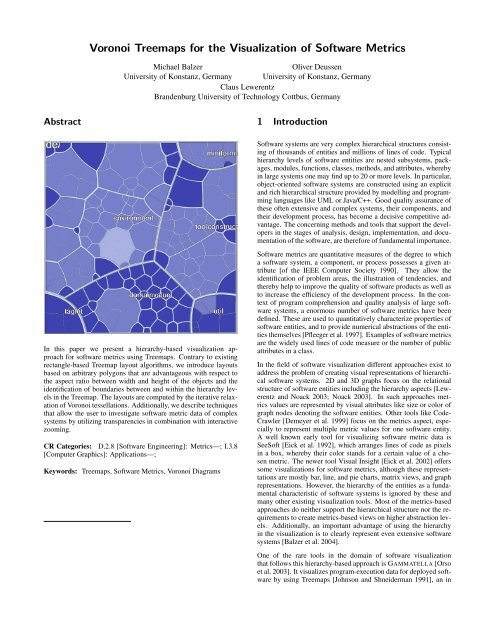
In this paper we present a method allowing us to generate Treemaps
consisting of arbitrary polygons that enable a meaningful visualization
of software metrics based on the hierarchy of a software
system. In the following section we address the data and the characteristics
of the visualized software metrics. In Section 3 previous
work on Treemaps is outlined. Our approach of Voronoi Treemaps
is presented in Section 4. Section 5 deals with assisting the user
in the exploration of the data in the Treemaps. Section 6 summarizes
our approach and discusses our future work. Examples of our
Voronoi Treemap visualizations of software metrics are shown in
Section 7.
2 Underlying Data
3 Previous Work on Treemaps
Treemaps were introduced by Shneiderman and Johnson in
1991 [Johnson and Shneiderman 1991]. Originally designed to visualize
files on a hard drive, Treemaps have been applied to a wide
variety of domains ranging from financial analysis [Jungmeister and
Turo 1992; Wattenberg 1998] to sports reporting [Jin and Banks
1997]. The basic idea is to subdivide a given area without producing
holes or overlappings. Therefore the area is alternately divided horizontally
and vertically according to the hierarchy of the objects and
the given proportion between the considered objects. Figure 2 illustrates
this method with a simple example. Each node has a name
and an associated size. The Treemap is constructed via recursive
subdivision of the initial rectangle. The size of each sub-rectangle
corresponds to the size of the node. The direction of the subdivision
alternates per level: first horizontally, next vertically, again
horizontally, etc. The initial rectangle is partitioned into smaller
rectangles, so that the size of each rectangle reflects the size of the
leaf. As a result of its construction, the Treemap reflects the structure
of the tree. This original Treemap layout algorithm is called
Slice-and-Dice.
Our structural models of object-oriented software distinguish five
types of software entities: packages, classes, methods, attributes,
and files. Each package can contain other packages, classes, and
files. Each class can contain other classes, methods, and attributes.
The schema of the models is shown in Figure 1.
Figure 2: Tree diagram and corresponding Treemap
Figure 1: Schema for hierarchical models of object-oriented software
systems
Such models can be automatically extracted from the source code
of object-oriented software systems. In our experiments we used
the tool Sotograph [Software-Tomography GmbH ] to extract the
models from Java programs. The extracted models are stored in
files in Rigi Standard Format [Wong 1998]. Through the separation
of extraction from visualization, and the use of a standard exchange
format, it is possible to visualize data from many sources. In particular,
they can be applied to software in any programming language
for which an appropriate extractor is available.
After extracting the models we possess a number of different software
metrics for the different entity types. They range from the
indication of size of the entities over the use by other entities, to
cyclic dependencies, and many more. All of them are quantitative
measures, which means that they can be counted, compared,
ordered, and summated. To represent these software metrics with
Treemaps, they are aggregated upward in the hierarchy. For example,
a class consists of several methods. All methods have a given
metric value that illustrates the number of calls of this method, and
the sum of calls of all contained methods is assigned to the class.
Likewise these metric values are propagated to the package level.
Thereby the user is able to identify the packages and classes with
frequently used methods immediately on a package or class level
without having to examine the methods directly.
A negative effect in these layouts is however, that the subdivision
in each step is solely done in one dimension. As result, thin elongated
rectangles with a high aspect ratio between width and height
emerge, if many objects or objects with high diversity in size are
considered. Such long rectangles are difficult to see, select, compare
in size, and label [Turo and Johnson 1992; Bruls et al. 2000].
Figure 3 presents an example.
This issue is addressed by Ordered Treemaps [Shneiderman and
Wattenberg 2001], Squarified Treemaps [Bruls et al. 2000], Clustered
Treemaps [Wattenberg 1999], and some other layout algorithms.
These layouts subdivide the area of the initial rectangle in
one step by both dimensions, meaning horizontally and vertically at
the same time. The main optimization criterion of these layout algorithms
is the approximation of the sub-rectangles to the shape of a
square, whereby the aspect ratio between width and height of each
rectangle converges to one. Aside from the aspect ratio criterion,
other criteria are considered as well. For example the order of the
objects or the nearness to a given point in the initial area, whereby
the other criteria are often closely related to the respective application
domain. A demonstrative member of this group of advanced
Treemap layout algorithms is presented in Figure 4, showing the
same data set as in Figure 3 with a Squarified Treemap layout that
is currently the favored layout algorithm for Treemaps.
Another problem in this group of algorithms is illustrated in Figure
4: it is hard to differentiate if two neighbor objects are siblings
or far away in the hierarchy. The problem is provoked by
the square-like shape of the rectangles, and because the edges are
only horizontally and vertically aligned, whereby the edges of the
different objects appear to run into each other. This effect may be
reduced, but can not be prevented by using borders and/or Cushion
Treemaps [van Wijk and van de Wetering 1999]. A solution for
this problem is the layout of Treemaps based on non-rectangular

Figure 3:
Treemaps
Aspect ratio problem of the original Slice-and-Dice
Figure 4:
Treemaps
Hierarchy level seperation problem of Squarified
objects. At this time such an approach does not exist, except in ET-
Maps [Roussinov and Chen 1998] where only composite shapes of
rectangles are assembled. So far all Treemap layouts are restricted
to axis-aligned rectangular shapes. Hence, we present our approach
for polygon-based Treemaps in the next section, in which Treemaps
with non-regulars shapes are generated.
4 Voronoi Treemaps
What are the constraints and optimization criteria for the shape
of Treemap objects? Firstly, the distribution of the objects must
fully utilize the given area, by avoiding holes and overlappings.
Secondly, the objects should distinguish themselves, meaning they
should have irregular shapes and the edges of the different objects
should not run into each other. Thirdly, the objects should be compact,
which means that the aspect ratio between their width and
height should converge to one.
Obviously polygons can be used. A polygon is defined as a closed
plane figure with n sides. Special cases of polygons are triangles
with n = 3, rectangles, squares, or quadrilaterals with n = 4, pentagons
with n = 5, and so on. Every polygon can be divided into
smaller polygons, hereby satisfying the first constraint. Polygons
can have arbitrary shapes and polygons with many edges can approximate
curves, which refers to the second and third optimization
criterion.
The principle structure of our layout algorithm is similar to the original
Treemap layout algorithm. The first step is to consider the objects
of the top level in the hierarchy. These objects are distributed
in the given area – mostly a rectangle, but other shapes are possible,
too. The output is a set of polygons. For the next hierarchy
level, this algorithm is performed recursively within the according
polygons of the considered objects in the hierarchy, and so on.
We now need a layout method, that allows us to divide a given area
into polygons under consideration of the given optimization criteria.
The basic idea is to use Voronoi tessellations. With their help,
we are able to perform an iterative relaxation of a specified number
of objects with corresponding sizes in a given polygonal area.
This method and the underlying theory of Voronoi tessellations is
explained in Section 4.1. However, here the problem is that for
the advanced Voronoi metric used by us, it is non-trivial to compute
the Voronoi tessellation analytically. For our application it is
quiet sufficient to compute an approximation on a numerical basis.
As a consequence thereof we must extract polygons out of this numerical
computed Voronoi tessellations. This step is explained in
Section 4.2. We need these polygons especially to perform the layout
in the next lower hierarchy level recursively and to display the
Treemap in general.
4.1 Centroidal Voronoi Tessellation
Let P := {p 1 ,...., p n } be a set of n distinct points, where 2 < n < ∞,
in R 2 with the coordinates (x p1 ,y p1 ),...,(x pn ,y pn ). These points are
the Voronoi sites. According to [de Berg et al. 2000; Okabe et al.
1992], we define the Voronoi tessellation of P as the subdivision
of R 2 into n cells, one for each site in P, with the property that
a point q lies in the cell corresponding to a site p i if and only if
distance(p i ,q) < distance(p j ,q) for each p i , p j ∈ P with i ≠ j. The
denotation distance(p,q) represents a specified distance function
between the two points p and q – mostly the Euclidian metric is
used, which is defined as
√
distance(p,q) := (x p − x q ) 2 + (y p − y q ) 2 ,
but others such as the Manhattan metric or the Maximum metric,
are possible as well. All points of a cell form a Voronoi polygon.
A Centroidal Voronoi Tessellation (CVT) [Du et al. 1999] is a
Voronoi tessellation of a given set, whereby the associated generating
points are centroids (centers of mass) of the corresponding
Voronoi polygons. These tessellations represent arrangements similar
to Poisson disc distributions. The CVT is computed by determining
the Voronoi tessellation of a given point set, then each point
is moved into the mass center of its assigned Voronoi polygon, and
these two steps are repeated iteratively until the error between all
point positions and the mass centers of their Voronoi polygons is
below a given ε. Figure 5 shows an example of a Voronoi tessellation
of 20 random points on the left, and the associated CVT on
the right – traces illustrate the movements of the points during the
computation of the CVT.

To further clarify the above procedure it should be noted, that firstly,
the radius of a circle may have values below zero – formally this object
is not a circle, but in our application this abstraction is useful
and even essential. Secondly, beside the mentioned simple adjustment
of the radius according to the area size error, it is necessary
to observe certain cases where the radius is or is nearby zero, and
where the radius needs to be switched from positive to negative, or
vice versa, to obtain better approximations.
Figure 5: Voronoi tessellation of 20 random points and the associated
CVT (traces illustrate the point movements during the computation
of the CVT)
With this basic CVT we are able to compute Treemap layouts in
which every leaf node in the hierarchy has the same value. However,
it is our goal to generate layouts in which the objects can have
different values. Hence we need to extend the distance metric by
adding a size parameter to every point. This corresponds to the
computation of Voronoi tessellations with circles as generator objects,
where the size parameter is the radius. The resulting distance
measure function is defined between a point q and a circle c with
the center p and the radius r as
distance(c,q) Circle := distance(p,q) − r.
Additionally, the radii of the circles are not specified by precise
values, but rather exist only as relations between all considered circles.
Their absolute radii result adaptively from the momentary positions
of the circles. This step is necessary because overlapping
circles would otherwise generate uncontinuous Voronoi polygons.
Therefore a maximum factor m is determined, so that no two circles
c 1 (p 1 ,r 1 ) and c 2 (p 2 ,r 2 ) exist with
distance(p 1 , p 2 ) − (r 1 + r 2 ) ∗ m < 0.
Factor m is then multiplied with the relative radius of each circle,
the result being the absolute radius. By creating CVTs fulfilling
these constraints, distributions of circles are developed under the
criterion of ’Maximum Growth’.
With this modified CVT we have not yet reached our goal, because
the values of the objects only correspond to the radii of the generator
circles and not to the sizes of the surface areas of the dedicated
Voronoi polygons. However, the key to success is to use the radii to
control the area sizes of the Voronoi polygons during the iterative
computation of the CVT. Analog to the modification of the position
in the classic CVT computation, we additionally change the
radius of every generator circle according to the relative size of the
Voronoi polygon to the total area size. For example, if the value
of an object in our hierarchy is 20% of the sum of all object values
in the current hierarchy level, but in the last iteration step the
dedicated Voronoi polygon covers only 16% of the overall area, we
will try to increase the area size of the Voronoi polygon in the next
iteration from 16% to 20% by increasing the radius of the generator
circle by 25%. Due to the facts that the relation between the radius
of a circle and the area size of the dedicated Voronoi polygon is not
a linear dependency, and the radii and positions of the other generator
circles are changing at the same time, we will most likely not
achieve the correct area size in the next step. However, we may presume
that a better approximation is obtained. By performing these
adjustments of the radii in every iteration step, the computation will
end up in a stable state, whereby the error between the designated
relative value of every object in the hierarchy and the relative area
size of the dedicated Voronoi polygon is below a given ε.
Figure 6 illustrates this iterative procedure with six objects, each
having a different value. After 104 iterations the Voronoi polygon
area size error δ A for every object was less than 0.01. At iteration
217 a stable state with a Voronoi polygon area size error δ A < 0.001
for every object was reached. During the computation the circles
have altered their sizes, relating to the changes of the positions and
radii of the other circles. The changing of the maximum area size
error of an object and the overall area size error is illustrated in
Figure 7. The computation time was less than one second on a
Pentium 4.
Figure 7: Convergence of the maximum area size error of an object
and the overall area size error during the computation of the CVT
in Figure 6. At a maximum error of δ A < 0.001 the computation
stopped.
As already mentioned in Section 4, it is non-trivial to compute this
Voronoi tessellations analytically, instead we calculate it numerically.
Hence, we use a set of sample points that is a CVT itself –
in compliance to the sampling theorem this produces much better
results than a regular grid or random points [Okabe et al. 1992].
The size of this set has to be appropriate for the number of generator
objects – in our experiments we used sets with sizes between
10’000 and 100’000 points. Before we start the computation of
the CVT, we first clip the set at the outer polygon that describes
the total available area for the current layout step. Following [Hoff
et al. 1999], in every iteration step for every sample we determine
the nearest circle according to the distance(c,q) Circle metric. Then,
for every circle we average the positions of the samples for which
the considered circle is the nearest to obtain the mass center of the
according Voronoi polygon. With this method we obtain good approximations
for Voronoi tessellations which satisfy the needs for
computing the CVT. Though this method is not precise enough to
extract the correct polygonal representations of the Voronoi cells.
Therefore we must use the method presented in the next section.

Figure 6: Iterative computation of a CVT of six objects with the Euclidian distance metric based on circles. A stable state with a Voronoi
polygon area size error δ A < 0.001 was reached in 217 steps. Iteration steps from top left to bottom right: 0 (start), 2, 6, 10, 14, 67, 76, 217
(end).
4.2 Polygon Extraction
After the CVT has been computed, we have to extract the Voronoi
polygons. Contrary to Section 4.1 we do not want to use a set of
sample points, because a polygon extraction on this basis produces
zigzag lines. Instead we will construct the curve segments between
the Voronoi cells directly. A curve segment e between two Voronoi
cells, specified by the two circles c 1 and c 2 , is defined as a set of
points P in R 2 where every p ∈ P fulfills the following two constraints:
After approximating the curves between all pairs of circles in the
manner described, we have to select the relevant curves. On a relevant
curve e(c 1 ,c 2 ) exists a point p with the property that for every
circle c i by i ∉ {1,2} distance(p,c i ) Circle > distance(p,c 1 ) Circle .
Non-relevant curves cannot contain curve segments for the Voronoi
tessellation due to the definitions in Section 4.1. The state after discarding
the non-relevant curves is illustrated in the center image in
Figure 8.
distance(p,c 1 ) Circle = distance(p,c 2 ) Circle ,
distance(p,c 1 ) Circle < distance(p,c i ) Circle for i ∉ {1,2}.
Obviously a curve segment between circles of the same radius is
a straight line, and between circles of different radius a parabola.
To construct these curve segments we determine all curves between
any two circles, select the relevant curves, clip them against each
other and the outer polygon, and finally merge them to polygons.
Since a polygon consists of a limited number of straight line edges,
it is adequate to choose a limited number of points p i ∈ P as well.
Given two circles c small and c large , a reasonable criterion is to sample
the curve by the angle α and the circle c small with r small ≤ r large .
This means to shoot n rays from p small , where the angle between
the rays t i and t i+1 is an adequate α, whereas t n+1 = t 1 . This
procedure enables a curvature-adaptive sampling. On every ray t
we calculate a point p which satisfies the first constraint for the
curve segment e(c small ,c large ), with the side constraint that for every
p i ∈ P distance(p i ,c small ) Circle > distance(p,c small ) Circle with
p ≠ p i , and distance(p,c small ) Circle < ∞. The connection of these
points according to the sampling order results in the designated
curve, which defines the border between the Voronoi cells of c small
and c large . The left image in Figure 8 shows these curves for every
pair of circles.
Figure 8: Extraction of Voronoi polygons: determining all curves
(left), discarding non-relevant curves (center), clipping (right)
The determined relevant curves are then clipped at the outer polygon
by starting from a point at the curve within the polygon, and
successively intersecting all edges of the curve with all edges of
the outer polygon in both directions of the starting point. If an
intersection is found on one side, all points beyond this intersection
are discarded, the intersection point is added to the curve, and
the search for intersections at the considered side of the polygon is
stopped. Now we have a set of relevant curve segments which are
completely within the outer polygon. In the next step the segments
are clipped taking the other segments into consideration. Following
the above constraint while looking for relevant curves, for every
segment we search one point whose two nearest neighbors are those
circles which have created this segment. Starting from this point,
we clip every edge of the segment e 1 (c 1 ,c 2 ) at all edges of the
other segments e i (c j ,c k ) at both sides of the starting point, whereby

i ≠ 1, and j ∈ {1,2} or k ∈ {1,2}. If an intersection is found on one
side, again all further points are discarded, the intersection point is
added, and the search at this side is stopped. The right image in
Figure 8 shows the segments after the clipping process.
Now we can assemble the final Voronoi polygons by combining the
remaining segments and the segments of the outer polygon. Instead
of looking for possible connection points, we utilize the fact that as
a result of the defined distance function each Voronoi polygon has
the following characteristic: the straight line edge between the center
of the circle that is associated to the Voronoi polygon and every
point of this polygon does not intersect any of the polygon edges.
Thus, we first calculate for each point p of the outer polygon the circle
c for which distance(p,c) Circle < distance(p,c i ) Circle for c ≠ c i ,
and add this point to the correspondent Voronoi polygon of circle
c. Then we sort all points of the segments and of the outer polygon
that are assigned to the respective circle by the angle of the straight
line edge between the center of the circle and the considered point.
Again it should be noted, that as a result of the curve sampling
step, the described polygon extraction method is an approximation
as well.
As the result we now have Voronoi polygons without holes and
overlappings within a given outer polygon, whereby the area size
of each polygon corresponds to the value of the assigned generator
object in the hierarchy. Furthermore, these polygons are clearly
distinguishable because of their irregular shapes, and their aspect
ratio converges to one. This fulfills the constraints and optimization
criteria of Treemaps, given in Section 4. Figure 9 presents the
final Voronoi Treemap layout computed with our approach.
Als already mentioned, software systems can be very complex.
Thus the Treemap layouts which represent the software metric data
of these systems will also be very complex. For this reason, we
developed and implemented two techniques for our software metric
data visualization tool. The first technique allows the user to interact
with the visualization. The second hides parts of the visualized
data so not to overwhelm the user with the mass of information.
The combination of these two techniques enables the effective examination
of large and complex data sets with thousands or even
millions of entities.
Interactive Zooming: With our tool the user is able to explore the
data analog to text based hierarchy browsers. At the beginning,
the complete Treemap is presented, starting at the top hierarchy
level. If the user is interested in a special part of the data he simply
clicks in this area, whereby the object in the next lower hierarchy
level relating to this area is selected. Following this selected object
is shown in full size on the screen. Again the user can select a
subarea for further investigation downwards the hierarchy, or he
can move back upwards the hierarchy. For not losing the context
in the visualization, the transition between two states is animated.
Figure 10 illustrates this interaction scheme – borders have been
added to every Voronoi polygon for a better differentiation between
the objects.
Figure 10: Zooming downwards and upwards the hierarchy
Figure 9: Final Voronoi Treemap layout with the same dataset as in
Figure 3 and 4
5 User interaction
Transparencies for Level-of-Detail: Using a hierarchy for the
software entities not only allows for better organizing them, but the
hierarchy is also designed to give an abstract view to components
of the software system. For that reason, it is not always desired to
inspect the system down to the last attribute, but rather it is necessary
to have these levels of abstraction in the visualization as well.
To realize this abstracted views we utilize transparencies similar
to [Balzer et al. 2004] in the following way: all objects at or above
the current hierarchy level are fully opaque. For every step down
the hierarchy, the transparency of the according objects is increased
by a given value δ t . If this value is equal to or below zero, all objects
on this level and all subordinate objects are not drawn. In the
rendering step after assigning the transparency values, all objects
are rendered in descending order according to the hierarchy, meaning
that the objects of the first level are rendered at first, then the
objects of the second level, and so on. The visual effect here is
that the objects further down the hierarchy seem to disappear and
objects which are 1/δ t or more levels down the hierarchy are hidden.
The change of the transparencies is animated when browsing
through the hierarchy as well, whereby objects not suddenly pop up
or disappear from one frame to another. In Figure 11 a data set with
different δ t is shown to demonstrate this information-based Levelof-Detail
technique.

7 Results
Finally, in the Figures 12 and 13 we want to present some demonstrative
results for software metric visualizations that are generated
with our Voronoi Treemap method including some additional information
about the represented data and the used metrics. A color
version can be found at the additional color plate.
The colors of the Treemap objects in the Figures 12 and 13 represent
the entity type of the according objects in the hierarchy of the
software system. Packages are light blue, classes are red, files are
yellow, methods are dark blue, and attributes are green. The color
of every object in the visualization is altered depending on the transparency
of the objects and the color of the occluded objects.
References
BALZER, M., NOACK, A., DEUSSEN, O., AND LEWERENTZ, C.
2004. Software landscapes: Visualizing the structure of large
software systems. In Joint Eurographics and IEEE TCVG Symposium
on Visualization, Eurographics Association, 261–266.
Figure 11: Using Transparencies for information-based Level-of-
Detail
Beside these two techniques we implemented an adaptive and selective
labeling and highlighting of the Treemap objects, which additionally
supports the user by finding the information he is looking
for. Examples are shown in the figures of Section 7.
6 Conclusions and Future Work
In this paper we presented an approach for visualizing software
metrics. We introduced a new method for computing layouts
of Treemaps, which are based on polygons and explained these
method in-depth. Additionally, we described techniques that allows
the user to investigate software metric data of complex software
systems. Aside the domain of software visualization this combination
of algorithms and techniques can also be used for other attributed
hierarchical data.
In an informal user study of students and colleagues, we observed
that the hierarchy and size parameters of the objects were better
recognized with our polygon-based Treemaps, than the established
algorithms presented in Section 3. Our estimation with regard to
the figure of the Treemap objects were confirmed, meaning that the
arbitrary shape of the polygons allows a much better differentiation
than rectangles.
In the current situation the computation for the Treemap layouts
is based on sampling. In this regard the computation is relatively
slow, which means that the time for generating layouts of complex
data sets with many thousand entities requires minutes instead of
seconds for the established layout algorithms. But in our opinion
this time is justifiable in reference to the obtained results.
Our future work will address three domains: firstly, we want to
adapt other metrics than the Euclidian distance measure to our algorithm.
Secondly, we aim for improving the polygon extraction
part by solving this problem analytically. Thirdly, as a final result
we want to integrate this technique in a software analysis environment.
BRULS, M., HUIZING, K., AND VAN WIJK, J. 2000. Squarified
treemaps. In Joint Eurographics and IEEE TCVG Symposium on
Visualization, IEEE Computer Society, 33–42.
DE BERG, M., VAN KREVELD, M., OVERMARS, M., AND
SCHWARZKOPF, O. 2000. Computational Geometry: Algorithms
and Applications, 2nd ed. Springer-Verlag, Berlin, Germany.
DEMEYER, S., DUCASSE, S., AND LANZA, M. 1999. A hybrid
reverse engineering approach combining metrics and program
visualization. In Proceedings of the 6th Working Conference on
Reverse Engineering, IEEE Computer Society, 175–186.
DU, Q., FABER, V., AND GUNZBURGER, M. 1999. Centroidal
voronoi tessellations: Applications and algorithms. SIAM Review
41, 4, 637–676.
EICK, S. G., STEFFEN, J. L., AND JR., E. E. S. 1992. Seesoft
- a tool for visualizing line oriented software statistics. IEEE
Transactions on Software Engineering 18, 11, 957–968.
EICK, S. G., GRAVES, T. L., KARR, A. F., MOCKUS, A., AND
SCHUSTER, P. 2002. Visualizing software changes. IEEE Transactions
on Software Engineering 28, 4, 396–412.
HOFF, K., KEYSER, J., LIN, M., MANOCHA, D., AND CULVER,
T. 1999. Fast computation of generalized voronoi diagrams
using graphics hardware. In Proceedings of the 26th Annual
Conference on Computer Graphics (SIGGRAPH), ACM Press,
277–286.
JIN, L., AND BANKS, D. C. 1997. Tennisviewer: A browser for
competition trees. IEEE Computer Graphics and Applications
17, 4, 63–65.
JOHNSON, B., AND SHNEIDERMAN, B. 1991. Tree maps: A
space-filling approach to the visualization of hierarchical information
structures. In IEEE Visualization, IEEE Computer Society,
284–291.
JUNGMEISTER, W.-A., AND TURO, D. 1992. Adapting treemaps
to stock portfolio visualization. Tech. Rep. UMCP-CSD CS-TR-
2996, University of Maryland, College Park, Maryland 20742,
U.S.A.

Figure 12: The left image visualizes the outbound calls of classes by other classes of the software system ‘ArgoUML’. The right image
visualizes the lines of code (LOC) of all files of the software system ‘JFree’.
LEWERENTZ, C., AND NOACK, A. 2003. Crococosmos – 3D visualization
of large object-oriented programs. In Graph Drawing
Software, M. Jünger and P. Mutzel, Eds. Springer-Verlag, 279–
297.
NOACK, A. 2003. An energy model for visual graph clustering.
In Proceedings of the 11th International Symposium on Graph
Drawing, Springer-Verlag, 425–436.
OF THE IEEE COMPUTER SOCIETY, S. C. C., 1990. IEEE standard
glossary of software engineering terminology. IEEE Std
610.12-1990.
OKABE, A., BOOTS, B., AND SUGIHARA, K. 1992. Spatial
Tessellations: Concepts and Applications of Voronoi Diagrams,
2nd ed. John Wiley and Sons Ltd.
ORSO, A., JONES, J. A., AND HARROLD, M. J. 2003. Visualization
of program-execution data for deployed software. In
Proceedings ACM 2003 Symposium on Software Visualization,
ACM Press, 67–76.
TURO, D., AND JOHNSON, B. 1992. Improving the visualization
of hierarchies with treemaps: Design issues and experimentation.
Tech. Rep. UMCP-CSD CS-TR-2901, University of Maryland,
College Park, Maryland 20742, U.S.A.
VAN WIJK, J. J., AND VAN DE WETERING, H. 1999. Cushion
treemaps: Visualization of hierarchical information. In Proceedings
of the IEEE Symposium on Information Visualization, IEEE
Computer Society, 73–78.
WATTENBERG, M., 1998. Map of the market,
http://smartmoney.com/marketmap.
WATTENBERG, M. 1999. Visualizing the stock market. In
Extended Abstracts on Human Factors in Computing Systems,
ACM Press, 188–189.
WONG, K. 1998. Rigi User’s Manual, Version 5.4.4.
http://ftp.rigi.csc.uvic.ca/pub/rigi/doc/.
PFLEEGER, S. L., JEFFERY, R., CURTIS, B., AND KITCHENHAM,
B. 1997. Status report on software measurement. IEEE Software
14, 2, 33–43.
ROUSSINOV, D., AND CHEN, H. 1998. A scalable self-organizing
map algorithm for textual classification: A neural network approach
to thesaurus generation. Communication and Cognition
15, 1-2, 81–112.
SHNEIDERMAN, B., AND WATTENBERG, M. 2001. Ordered
treemap layouts. In Proceedings of the IEEE Symposium on Information
Visualization, IEEE Computer Society, 73–78.
SOFTWARE-TOMOGRAPHY
http://www.softwaretomography.com.
GMBH.

Figure 13: Visualization of the static structure of packages, classes, methods, and attributes of the software system ‘JFree’. The top image
uses the Treemap algorithm presented in this paper, the lower left uses the Slice-and-Dice algorithm, and the lower right is computed with
the Squarified Treemap algorithm.