Cloud Statistics from Calipso Lidar Data for the ... - espace-tum.de
Cloud Statistics from Calipso Lidar Data for the ... - espace-tum.de
Cloud Statistics from Calipso Lidar Data for the ... - espace-tum.de

You also want an ePaper? Increase the reach of your titles
YUMPU automatically turns print PDFs into web optimized ePapers that Google loves.
Technische Universität München<br />
Master’s Thesis<br />
<strong>Cloud</strong> <strong>Statistics</strong> <strong>from</strong> <strong>Calipso</strong> <strong>Lidar</strong><br />
<strong>Data</strong> <strong>for</strong> <strong>the</strong> Per<strong>for</strong>mance Assessment of<br />
a Methane Space <strong>Lidar</strong><br />
Author:<br />
Nico Trebbin<br />
Supervisor:<br />
Dr. Christoph Kiemle<br />
A <strong>the</strong>sis submitted in fulfillment of <strong>the</strong> requirements<br />
<strong>for</strong> <strong>the</strong> <strong>de</strong>gree of Master of Science<br />
in <strong>the</strong><br />
Earth Oriented Space Science and Technology<br />
Master’s Program<br />
October 2013
Declaration of Authorship<br />
I, Nico Trebbin, <strong>de</strong>clare that this <strong>the</strong>sis titled, ’<strong>Cloud</strong> <strong>Statistics</strong> <strong>from</strong> <strong>Calipso</strong> <strong>Lidar</strong> <strong>Data</strong><br />
<strong>for</strong> <strong>the</strong> Per<strong>for</strong>mance Assessment of a Methane Space <strong>Lidar</strong>’ and <strong>the</strong> work presented in<br />
it are my own. I confirm that:<br />
<br />
This work was done wholly or mainly while in candidature <strong>for</strong> a research <strong>de</strong>gree<br />
at this University.<br />
<br />
Where any part of this <strong>the</strong>sis has previously been submitted <strong>for</strong> a <strong>de</strong>gree or any<br />
o<strong>the</strong>r qualification at this University or any o<strong>the</strong>r institution, this has been clearly<br />
stated.<br />
<br />
Where I have consulted <strong>the</strong> published work of o<strong>the</strong>rs, this is always clearly attributed.<br />
<br />
Where I have quoted <strong>from</strong> <strong>the</strong> work of o<strong>the</strong>rs, <strong>the</strong> source is always given. With<br />
<strong>the</strong> exception of such quotations, this <strong>the</strong>sis is entirely my own work.<br />
<br />
I have acknowledged all main sources of help.<br />
<br />
Where <strong>the</strong> <strong>the</strong>sis is based on work done by myself jointly with o<strong>the</strong>rs, I have ma<strong>de</strong><br />
clear exactly what was done by o<strong>the</strong>rs and what I have contributed myself.<br />
Signed:<br />
Date of Submission:<br />
iii
”Science never solves a problem without creating ten more.”<br />
George Bernard Shaw
TECHNISCHE UNIVERSITÄT MÜNCHEN<br />
Abstract<br />
Ingenieurfakultät Bau Geo Umwelt<br />
Master of Science<br />
<strong>Cloud</strong> <strong>Statistics</strong> <strong>from</strong> <strong>Calipso</strong> <strong>Lidar</strong> <strong>Data</strong> <strong>for</strong> <strong>the</strong> Per<strong>for</strong>mance Assessment<br />
of a Methane Space <strong>Lidar</strong><br />
by Nico Trebbin<br />
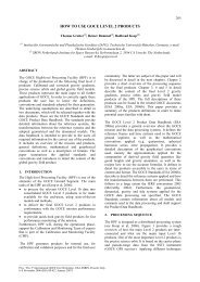
In this <strong>the</strong>sis a per<strong>for</strong>mance assessment <strong>for</strong> <strong>the</strong> future German-French climate monitoring<br />
initiative, Methane Remote Sensing <strong>Lidar</strong> Mission (MERLIN), proposed by DLR and<br />
CNES in 2010 was un<strong>de</strong>rtaken. A general space lidar per<strong>for</strong>mance issue is <strong>the</strong> obstruction<br />
by optically <strong>de</strong>nse clouds. For this purpose cloud free statistics, <strong>the</strong> global cloud top<br />
flatness and global cloud top distributions were <strong>de</strong>rived <strong>from</strong> <strong>the</strong> <strong>Cloud</strong>-Aerosol <strong>Lidar</strong><br />
and Infrared Pathfin<strong>de</strong>r Satellite Observation (CALIPSO) level 2, 333 m and 5 km lidar<br />
cloud-layer products between 01 January 2007 and 01 January 2008. Merging both data<br />
sets toge<strong>the</strong>r <strong>the</strong>reby allowed <strong>the</strong> best possible simulation of near global and seasonal<br />
real world atmospheric conditions that a spaceborne Integrated Path Differential Absorption<br />
(IPDA) lidar like MERLIN will encounter. With 40.5 % overall global cloud<br />
free fraction, a cloud gap distribution which is following a power-law distribution with<br />
exponent α = 1.51 ± 0.01 toge<strong>the</strong>r with a mean cloud gap length of 7.41 km and about<br />
200 daily global cloud top flatness events, <strong>the</strong> analysis reveals a dominance of small<br />
cloud gaps which is confirmed by a low median cloud gap length of only 1 km. While<br />
<strong>the</strong> cloud free fraction results were compared and confirmed with Aqua Mo<strong>de</strong>rate Resolution<br />
Imaging Spectroradiometer (MODIS) seasonal and annual cloud fraction data,<br />
<strong>the</strong> power-law distribution of cloud gaps was confirmed by an extensive statistical analysis<br />
using maximum likelihood estimation, Kolmogorov-Smirnov statistics and likelihood<br />
ratio tests. Taking 605 x 10 8 individual CALIPSO measurements of <strong>the</strong> year 2007 with<br />
a horizontal resolution of 333 m and computing cloud gap and cloud free statistics <strong>for</strong> 2 ◦<br />
x 2 ◦ latitu<strong>de</strong>/longitu<strong>de</strong> grid points <strong>the</strong>reby i<strong>de</strong>ntified regional and seasonal changes in<br />
<strong>the</strong> probability of spaceborne lidar surface <strong>de</strong>tection. The analysis reveals that MERLIN<br />
will be able to per<strong>for</strong>m near global methane mixing ratio column retrievals.
Acknowledgements<br />
I would like to thank ICARE <strong>for</strong> providing me <strong>the</strong> CALIPSO data through <strong>the</strong>ir FTP<br />
server, Dr. Christoph Kiemle <strong>for</strong> his superior supervision, Dr. Axel Amediek, Dr.<br />
Mathieu Quatrevalet and Dr. Stephan Kox <strong>for</strong> <strong>the</strong> consultation in preparation of <strong>the</strong><br />
<strong>the</strong>sis and <strong>the</strong> <strong>de</strong>velopers of Python, NumPy, Matplotlib, Basemap, PyHDF, h5Py,<br />
powerlaw and PyQt <strong>for</strong> providing me with an excellent software basis <strong>for</strong> <strong>de</strong>veloping <strong>the</strong><br />
software used within this <strong>the</strong>sis.<br />
ix
Contents<br />
Declaration of Authorship<br />
iii<br />
Abstract<br />
vii<br />
Acknowledgements<br />
ix<br />
List of Figures<br />
List of Tables<br />
Abbreviations<br />
SI Units and Abbreviations<br />
Symbols<br />
xiii<br />
xv<br />
xvii<br />
xix<br />
xxi<br />
1 Introduction and motivation 1<br />
1.1 The MERLIN mission . . . . . . . . . . . . . . . . . . . . . . . . . . . . . 1<br />
1.1.1 Methane as an important trace-gas . . . . . . . . . . . . . . . . . . 1<br />
1.1.2 The global methane budget . . . . . . . . . . . . . . . . . . . . . . 3<br />
1.1.3 In-situ measurements and remote sensing . . . . . . . . . . . . . . 3<br />
1.1.4 Scientific challenges and measurement strategy . . . . . . . . . . . 6<br />
1.2 The CALIPSO mission . . . . . . . . . . . . . . . . . . . . . . . . . . . . . 8<br />
1.2.1 Global cloud coverage by lidar measurements <strong>from</strong> space . . . . . . 8<br />
1.2.2 Scientific challenges and limits of CALIPSO . . . . . . . . . . . . . 8<br />
1.3 Goals . . . . . . . . . . . . . . . . . . . . . . . . . . . . . . . . . . . . . . 10<br />
2 Background in<strong>for</strong>mation and methodology of CALIPSO 11<br />
2.1 The fundamental equations . . . . . . . . . . . . . . . . . . . . . . . . . . 11<br />
2.2 The CALIOP payload . . . . . . . . . . . . . . . . . . . . . . . . . . . . . 15<br />
2.3 The <strong>Cloud</strong> Detection Algorithm of CALIPSO . . . . . . . . . . . . . . . . 16<br />
2.4 CALIPSO data sets . . . . . . . . . . . . . . . . . . . . . . . . . . . . . . 18<br />
2.5 CALIPSO lidar surface return . . . . . . . . . . . . . . . . . . . . . . . . . 22<br />
3 Methodology behind cloud free and cloud gap statistics 24<br />
xi
Contents<br />
xii<br />
3.1 Introduction . . . . . . . . . . . . . . . . . . . . . . . . . . . . . . . . . . . 24<br />
3.2 <strong>Data</strong> Reading and Merging . . . . . . . . . . . . . . . . . . . . . . . . . . 26<br />
3.3 Processing and algorithm . . . . . . . . . . . . . . . . . . . . . . . . . . . 29<br />
3.4 Visualization and Analysis . . . . . . . . . . . . . . . . . . . . . . . . . . . 33<br />
4 Case studies 35<br />
4.1 Typical broken cloud scene . . . . . . . . . . . . . . . . . . . . . . . . . . 36<br />
4.2 Multilayered cloud scene . . . . . . . . . . . . . . . . . . . . . . . . . . . . 37<br />
4.3 Multilayered cloud flatness scene . . . . . . . . . . . . . . . . . . . . . . . 38<br />
4.4 Low maritime flat cloud scene . . . . . . . . . . . . . . . . . . . . . . . . . 39<br />
5 <strong>Cloud</strong> free statistics 40<br />
5.1 Global cloud free fraction . . . . . . . . . . . . . . . . . . . . . . . . . . . 40<br />
5.2 Global cloud gap frequency . . . . . . . . . . . . . . . . . . . . . . . . . . 45<br />
5.3 Global cloud gap distribution . . . . . . . . . . . . . . . . . . . . . . . . . 52<br />
5.4 Conclusion . . . . . . . . . . . . . . . . . . . . . . . . . . . . . . . . . . . 56<br />
6 <strong>Cloud</strong> flatness occurrence 57<br />
6.1 Search criteria and algorithm . . . . . . . . . . . . . . . . . . . . . . . . . 57<br />
6.2 Global cloud flatness occurrence . . . . . . . . . . . . . . . . . . . . . . . 59<br />
6.3 Low maritime clouds . . . . . . . . . . . . . . . . . . . . . . . . . . . . . . 61<br />
6.4 Conclusion . . . . . . . . . . . . . . . . . . . . . . . . . . . . . . . . . . . 63<br />
7 <strong>Cloud</strong> top height distribution 64<br />
7.1 Global cloud top height distribution . . . . . . . . . . . . . . . . . . . . . 64<br />
7.2 Conclusion . . . . . . . . . . . . . . . . . . . . . . . . . . . . . . . . . . . 68<br />
8 Conclusion 69<br />
8.1 Space lidar <strong>for</strong> methane measurements . . . . . . . . . . . . . . . . . . . . 69<br />
8.2 Estimated measurement <strong>de</strong>nsity . . . . . . . . . . . . . . . . . . . . . . . . 70<br />
8.3 Outlook . . . . . . . . . . . . . . . . . . . . . . . . . . . . . . . . . . . . . 72<br />
A Detailed results and additional in<strong>for</strong>mation 73<br />
Bibliography 80
List of Figures<br />
1 Global methane networks . . . . . . . . . . . . . . . . . . . . . . . . . . . 5<br />
2 MERLIN measurement principle . . . . . . . . . . . . . . . . . . . . . . . 7<br />
3 Scattering by an spherical i<strong>de</strong>alized particle . . . . . . . . . . . . . . . . . 13<br />
4 <strong>Calipso</strong> L2 algorithms . . . . . . . . . . . . . . . . . . . . . . . . . . . . . 18<br />
5 <strong>Calipso</strong> L2 data sets . . . . . . . . . . . . . . . . . . . . . . . . . . . . . . 20<br />
6 Surface lidar returns of <strong>the</strong> 333 m layer product . . . . . . . . . . . . . . . 23<br />
7 Diagram of <strong>Calipso</strong> <strong>Statistics</strong> components . . . . . . . . . . . . . . . . . . 25<br />
8 File name convention . . . . . . . . . . . . . . . . . . . . . . . . . . . . . . 27<br />
9 Normed total number of measurements . . . . . . . . . . . . . . . . . . . . 28<br />
10 Merging algorithm of <strong>the</strong> analyzed data set . . . . . . . . . . . . . . . . . 30<br />
11 Diagram of algorithms used <strong>for</strong> <strong>the</strong> analysis . . . . . . . . . . . . . . . . . 33<br />
12 Typical broken cloud scene . . . . . . . . . . . . . . . . . . . . . . . . . . 36<br />
13 Multilayered cloud scene . . . . . . . . . . . . . . . . . . . . . . . . . . . . 37<br />
14 Multilayered cloud flatness scene . . . . . . . . . . . . . . . . . . . . . . . 38<br />
15 Low maritime flat cloud scene . . . . . . . . . . . . . . . . . . . . . . . . . 39<br />
16 Total cloud free fraction <strong>for</strong> 2007 . . . . . . . . . . . . . . . . . . . . . . . 41<br />
17 Total cloud free fraction <strong>for</strong> different seasons of 2007 . . . . . . . . . . . . 42<br />
18 <strong>Cloud</strong> free fraction averaged over latitu<strong>de</strong> <strong>de</strong>gree <strong>for</strong> 2007 . . . . . . . . . 44<br />
19 Occurrence frequency of cloud gap lengths <strong>for</strong> 2007 . . . . . . . . . . . . . 46<br />
20 Best fit power law of cloud gaps <strong>for</strong> 2007 . . . . . . . . . . . . . . . . . . . 49<br />
21 Mo<strong>de</strong>l PDF of cloud gap lengths <strong>for</strong> 2007 . . . . . . . . . . . . . . . . . . 50<br />
22 Global cloud gap power law fit <strong>for</strong> 2007 . . . . . . . . . . . . . . . . . . . 53<br />
23 Total number and <strong>the</strong>ir respective mean of cloud gaps <strong>for</strong> 2007 . . . . . . 54<br />
24 Median of cloud gap lengths <strong>for</strong> 2007 . . . . . . . . . . . . . . . . . . . . . 55<br />
25 <strong>Cloud</strong> flatness search algorithm . . . . . . . . . . . . . . . . . . . . . . . . 58<br />
26 Total cloud top flatness events <strong>for</strong> 2007 . . . . . . . . . . . . . . . . . . . 60<br />
27 Seasonal cloud flatness events . . . . . . . . . . . . . . . . . . . . . . . . . 61<br />
28 <strong>Cloud</strong> <strong>for</strong>mation process over <strong>the</strong> ocean . . . . . . . . . . . . . . . . . . . 63<br />
29 Global cloud top height distribution histogram <strong>for</strong> 2007 . . . . . . . . . . 65<br />
30 Global cloud top height distribution <strong>for</strong> 2007 . . . . . . . . . . . . . . . . 66<br />
31 Global cloud height distribution <strong>for</strong> different seasons of 2007 . . . . . . . . 68<br />
32 Overall estimated per<strong>for</strong>mance of a space lidar . . . . . . . . . . . . . . . 71<br />
xiii
List of Figures<br />
xiv<br />
33 Global cloud gap power law fit uncertainties . . . . . . . . . . . . . . . . . 76<br />
34 Global cloud flatness events <strong>for</strong> different seasons of 2007 . . . . . . . . . . 77<br />
36 Global cloud height distribution <strong>for</strong> different seasons of 2007 . . . . . . . . 79
List of Tables<br />
1 Key MERLIN parameters . . . . . . . . . . . . . . . . . . . . . . . . . . . 7<br />
2 Key CALIPSO parameters . . . . . . . . . . . . . . . . . . . . . . . . . . . 9<br />
3 Comparison of 333m, 1km and 5km product . . . . . . . . . . . . . . . . . 21<br />
4 <strong>Cloud</strong> free fraction part <strong>for</strong> <strong>the</strong> validation study of January 2007 . . . . . 31<br />
5 Distance of geographical <strong>de</strong>grees . . . . . . . . . . . . . . . . . . . . . . . 32<br />
6 Key properties of analyzed data set . . . . . . . . . . . . . . . . . . . . . . 40<br />
7 <strong>Cloud</strong> free fraction averaged by latitudal zones and compared to MODIS . 43<br />
8 Power law fits <strong>for</strong> different methods and <strong>for</strong> <strong>the</strong> discrete and continuous<br />
case . . . . . . . . . . . . . . . . . . . . . . . . . . . . . . . . . . . . . . . 50<br />
9 Log-likelihood ratios and <strong>the</strong>ir probability <strong>for</strong> selected power law fits . . . 52<br />
10 Total number of cloud flatness events <strong>for</strong> 2007 . . . . . . . . . . . . . . . . 59<br />
11 1/3 km <strong>Cloud</strong> Layer and Column Descriptor Record . . . . . . . . . . . . 74<br />
12 5 km <strong>Cloud</strong> Layer and Column Descriptor Record . . . . . . . . . . . . . 74<br />
13 <strong>Cloud</strong>less fraction averaged by latitudal zones<strong>for</strong> 2007 . . . . . . . . . . . 75<br />
xv
Abbreviations<br />
ABL<br />
ATBD<br />
BSP<br />
CALIOP<br />
CALIPSO<br />
CCDF<br />
CDF<br />
CNES<br />
CPR<br />
DLR<br />
EarthCARE<br />
ECMWF<br />
ENVISAT<br />
EOS<br />
ESA<br />
FOV<br />
GAW<br />
GLAS<br />
GOSAT<br />
ICARE<br />
IPDA<br />
IIR<br />
IPA<br />
ITCZ<br />
LITE<br />
Atmospheric boundary layer<br />
Algorithm Theoretical Basis Document<br />
Backscatter profiles<br />
<strong>Cloud</strong>-Aerosol <strong>Lidar</strong> with Orthogonal Polarization<br />
<strong>Cloud</strong>-Aerosol <strong>Lidar</strong> and Infrared Pathfin<strong>de</strong>r Satellite Observations<br />
Complementary cumulative distribution function<br />
Cumulative distribution function<br />
Centre National d’Etu<strong>de</strong>s Spatiales<br />
<strong>Cloud</strong> Profiling Radar<br />
Deutsches Zentrum für Luft- und Raumfahrt<br />
Earth <strong>Cloud</strong>s, Aerosols and Radiation Explorer<br />
European Centre <strong>for</strong> Medium-Range Wea<strong>the</strong>r Forecasts<br />
Enviromental Satellite<br />
Earth Observing System<br />
European Space Agency<br />
Field of view<br />
Global Atmosphere Watch<br />
Geoscience Laser Altimeter System<br />
Greenhous Gases Observing Satellite<br />
<strong>Cloud</strong>-Aerosol-Water-Radiation Interactions<br />
Integrated Path Differential Absorption<br />
Infrared Imaging Radiometer<br />
Institut für Physik <strong>de</strong>r Atmosphäre<br />
Intertropical convergence zone<br />
LIDAR In-Space Technology Experiment<br />
xvii
Abbreviations<br />
xviii<br />
LaRC<br />
MERLIN<br />
MODIS<br />
NASA<br />
PCFLOS<br />
NOAA<br />
PDF<br />
PSC<br />
SNR<br />
TOA<br />
TTL<br />
UTC<br />
VFM<br />
WDCGG<br />
WFC<br />
WMO<br />
Langley Research Center<br />
Methane Remote Sensing <strong>Lidar</strong> Mission<br />
Mo<strong>de</strong>rate Resolution Imaging Spectroradiometer<br />
National Aeronautics and Space Administration<br />
Probability of cloud free line-of-sight<br />
National Oceanic and Atmospheric Administration<br />
Probability <strong>de</strong>nsity function<br />
Polar stratospheric cloud<br />
Signal-to-noise ratio<br />
Top of <strong>the</strong> atmosphere<br />
Tropical Tropopause Layer<br />
Universal Time Conversion<br />
Vertical Feature Mask<br />
World <strong>Data</strong> Centre <strong>for</strong> Greenhause Gases<br />
Wi<strong>de</strong> Field Camera<br />
World Meteorological Organization
SI Units and Abbreviations<br />
<strong>de</strong>g <strong>de</strong>gree<br />
◦ C<br />
J<br />
K<br />
km<br />
m<br />
ms<br />
nm<br />
per, %<br />
<strong>de</strong>gree Celsius<br />
joule<br />
kelvin<br />
kilometer<br />
meter<br />
millisecond<br />
nanometer<br />
percent<br />
s, sec second<br />
sr steradian<br />
V volt<br />
W watt<br />
µm micron, micrometer<br />
float32<br />
float64<br />
GB<br />
int8<br />
int16<br />
int32<br />
MB<br />
uint8<br />
uint16<br />
uint32<br />
floating point, 32 bits or 4 bytes<br />
floating point, 64 bits or 8 bytes<br />
Gbyte, gigabyte, 10 9 byte<br />
integer, 8 bits or 1 byte<br />
integer, 16 bits or 2 bytes<br />
integer, 32 bits or 4 bytes<br />
Mbyte, megabyte, 10 6 byte<br />
unsigned integer, 8 bits or 1 byte<br />
unsigned integer, 16 bits or 2 bytes<br />
unsigned integer, 32 bits or 4 bytes<br />
xix
Symbols<br />
c gap cloud gap km<br />
C Lay cloud layer No Unit<br />
f c cloud fraction No Unit<br />
f cf cloud free fraction No Unit<br />
z t cloud top height km<br />
z b cloud base height km<br />
α power law exponent No Unit<br />
β backscatter coefficient km −1 sr −1<br />
λ wavelength nm<br />
σ significant error No Unit<br />
τ optical thickness No Unit<br />
xxi
Dedicated to <strong>the</strong> ones I love and to <strong>the</strong> only planet inhabiting<br />
seven billion people that someday might change <strong>the</strong>ir mind and<br />
stop wrecking <strong>the</strong>mselves and <strong>the</strong> nature <strong>the</strong>y are living in.<br />
xxiii
Chapter 1<br />
Introduction and motivation<br />
1.1 The MERLIN mission<br />
1.1.1 Methane as an important trace-gas<br />
Methane (CH 4 ), which occurs at about 1800 ppb (parts per billion which ̂= nmol mol −1 ,<br />
dry air mixing ratio) by volume in <strong>the</strong> atmosphere of Earth (http://www.esrl.noaa.<br />
gov/gmd/aggi/aggi.html), is consi<strong>de</strong>red <strong>the</strong> second most important anthropogenic<br />
greenhouse gas after CO 2 . According to <strong>the</strong> US National Oceanic and Atmospheric<br />
Administration (NOAA), methane is 21 times more effective at trapping heat in <strong>the</strong> atmosphere<br />
than CO 2 by weight, over a 100-year period. Present estimates of 2012 are that<br />
methane accounts <strong>for</strong> 0.507 W m −2 radiative <strong>for</strong>cing which equals about 17.5% of <strong>the</strong><br />
total <strong>for</strong>cing potential of all long-lived greenhouse gases. Although atmospheric methane<br />
levels were almost constant <strong>from</strong> 1999 to 2006, <strong>the</strong> CH 4 globally averaged concentration<br />
in <strong>the</strong> atmosphere started rising again. Causes <strong>for</strong> this recent increase inclu<strong>de</strong> an Arctic<br />
warm period in 2007 and increased precipitation in <strong>the</strong> tropics <strong>for</strong> a period <strong>from</strong> 2007<br />
to 2008. Fortunately, near-zero growth in <strong>the</strong> Arctic during 2008 suggests that climate<br />
feedbacks as a result of melting permafrost and nascent CH 4 hydrates have not been<br />
activated yet [Dlugokencky et al., 2009]. Those CH 4 hydrates are on <strong>the</strong> one hand stored<br />
on <strong>the</strong> seabed along continental margins where <strong>the</strong>y are stabilized by high pressure and<br />
low temperatures and on <strong>the</strong> o<strong>the</strong>r hand in soils trapped by <strong>the</strong> overlying ice sheet of <strong>the</strong><br />
permafrost. Implying a global warming could lead to a hydrate instability in <strong>the</strong> oceans<br />
due to ocean warming and a melting of permafrost regions, which consequently would<br />
result in an additional release of methane into <strong>the</strong> atmosphere [Forster et al., 2007].<br />
As <strong>the</strong> global abundance of atmospheric methane increased by a factor of 2.5 since 1750<br />
[Dlugokencky et al., 2011] one reason <strong>for</strong> scientists to conduct methane analysis is to<br />
1
Chapter 1. Introduction and motivation 2<br />
assess methane emissions in response to large-scale climate change events in <strong>the</strong> past.<br />
While palaeorecords can help to i<strong>de</strong>ntify <strong>the</strong> global long term trend and can project<br />
what to expect in <strong>the</strong> future, present-day analysis is important to i<strong>de</strong>ntify natural and<br />
anthropogenic sources of methane emissions such as wetlands and CH 4 hydrates, fossil<br />
fuel exploitation, waste management and biomass burning. Implying a constant increase<br />
in <strong>the</strong> world population and living standards could also lead to additional anthropogenic<br />
methane emissions in <strong>the</strong> future. Besi<strong>de</strong>s that, <strong>the</strong> predicted global warming may increase<br />
natural methane emissions due to a positive feedback on <strong>the</strong> climate system.<br />
As <strong>the</strong> regions that contribute generally to natural and anthropogenic atmospheric<br />
methane have been i<strong>de</strong>ntified and <strong>the</strong> existing sampling coverage is sufficient to capture<br />
large-scale zonally averaged features, precise regional assessments are not possible<br />
yet. Current climate mo<strong>de</strong>ls use inverse calculations [Zhao et al., 2009] and extrapolation<br />
<strong>from</strong> a relatively small number of direct measurements <strong>from</strong> ground networks<br />
or <strong>from</strong> satellites [Bergamaschi et al., 2013] to estimate methane emissions. This data<br />
has obvious value, but due to <strong>the</strong> loss of ENVISAT in April 2012 and to <strong>the</strong> last remaining<br />
CH 4 observing satellite GOSAT (http://www.jaxa.jp/projects/sat/gosat/<br />
in<strong>de</strong>x_e.html), it could be improved significantly with wi<strong>de</strong>spread additional accurate<br />
measurements. While present measurements of methane <strong>from</strong> satellites rely on passive<br />
remote sensing with spectrometers which are <strong>de</strong>pen<strong>de</strong>nt on sunlight conditions and<br />
generally suffer <strong>from</strong> low measurement sensitivity in <strong>the</strong> lower troposphere close to <strong>the</strong><br />
methane sources, additional measurements <strong>from</strong> active remote sensing satellites will help<br />
reduce uncertainty in climate mo<strong>de</strong>ls and lead to a more comprehensive un<strong>de</strong>rstanding<br />
of <strong>the</strong> CH 4 sources [Kiemle et al., 2011].<br />
In addition to <strong>the</strong> general scientific interest, methane monitoring is and will be an important<br />
component of a greenhouse gas regulatory framework, as agreed in <strong>the</strong> Kyoto<br />
protocol which was exten<strong>de</strong>d until 2020. To achieve <strong>the</strong> goals of <strong>the</strong> protocol, a continuous<br />
global high-resolution monitoring of all greenhouse gases is required and <strong>the</strong><br />
i<strong>de</strong>ntification of discrepancies and fraudulent activities of countries who ratified <strong>the</strong> protocol<br />
is, besi<strong>de</strong>s <strong>the</strong> scientific aspect, one of <strong>the</strong> most important reasons of an extension<br />
of monitoring capabilities. The German-French climate initiative [Stephan et al., 2011]<br />
with <strong>the</strong> Methane Remote Sensing <strong>Lidar</strong> Mission (MERLIN) is inten<strong>de</strong>d to help reduce<br />
monitoring uncertainties. It will <strong>for</strong> <strong>the</strong> first time utilize a space-based active differential<br />
absorption lidar, which is particularly sensitive near <strong>the</strong> methane sources, while<br />
being in<strong>de</strong>pen<strong>de</strong>nt of sunlight, offering high and quantifiable accuracy and providing <strong>the</strong><br />
community with near-global measurements.
Chapter 1. Introduction and motivation 3<br />
1.1.2 The global methane budget<br />
Both greenhouse gases CO 2 and CH 4 play roles in <strong>the</strong> natural and anthropogenic cycle<br />
of carbon, involving continuous flows of large amounts of carbon among <strong>the</strong> ocean, <strong>the</strong><br />
terrestrial biosphere and <strong>the</strong> atmosphere. By photosyn<strong>the</strong>sis, plants and <strong>the</strong> terrestrial<br />
biosphere convert carbon (especially CO 2 ) into biomass and plant growth and <strong>the</strong>reby<br />
<strong>de</strong>crease <strong>the</strong> atmospheric concentration of CO 2 . Additionally, carbon dioxi<strong>de</strong> dissolves<br />
directly <strong>from</strong> <strong>the</strong> atmosphere by <strong>for</strong>ming carbonic acid during <strong>the</strong> reaction with water<br />
bodies (e.g. oceans, lakes, etc.) which <strong>the</strong>n can be absorbed by rocks through wea<strong>the</strong>ring<br />
or simply being washed into <strong>the</strong> ocean. The major removal mechanism of CH 4<br />
<strong>from</strong> <strong>the</strong> atmosphere is its reaction with <strong>the</strong> hydroxyl radical OH in <strong>the</strong> troposphere<br />
and stratosphere. However, plant, soil and animal respiration as well as <strong>de</strong>composition<br />
of <strong>de</strong>ad biomass, return carbon to <strong>the</strong> atmosphere as CO 2 or as CH 4 by microorganisms<br />
un<strong>de</strong>r anaerobic conditions. While <strong>the</strong> cycle of plant photosyn<strong>the</strong>sis, biomass production<br />
and <strong>de</strong>cay of <strong>de</strong>ad organic matter was stable until 1750, <strong>the</strong> injection of additional CO 2<br />
and CH 4 gases into <strong>the</strong> atmosphere by land use, <strong>de</strong><strong>for</strong>estation and fossil fuel burning<br />
disturbed <strong>the</strong> stability of <strong>the</strong> cycle [Forster et al., 2007]. Taking into account <strong>the</strong> relatively<br />
short lifetime of CH 4 in <strong>the</strong> atmosphere of approximately nine years, <strong>the</strong> accurate<br />
<strong>de</strong>tection of methane sources could lead to a mitigation of at least fur<strong>the</strong>r anthropogenic<br />
emissions. While emissions of CH 4 <strong>from</strong> wetlands vary significantly <strong>de</strong>pending on meteorological<br />
conditions [Dlugokencky et al., 2011], and o<strong>the</strong>r natural sources such as<br />
termites, oceans, wild fires, and wild ruminant animals remain in balance according to<br />
pre-industrial atmospheric CH 4 abundance, mainly anthropogenic sources contribute to<br />
<strong>the</strong> rise in atmospheric concentration. These man-ma<strong>de</strong> methane sources are generated<br />
by crushing, transmission, distribution and processing <strong>from</strong> coal, oil and gas extraction,<br />
as well as agricultural sources such as rice cultivation, domesticated animals and biomass<br />
burning. Additionally leaky waste disposals account <strong>for</strong> a total of approximately 230-<br />
467 Tg CH 4 yr −1 (1 Tg = 10 12 g) emitted by anthropogenic sources. Compared to <strong>the</strong><br />
124-275 Tg CH 4 yr −1 naturally emitted methane which are expected to remain constant<br />
[Forster et al., 2007], it is obvious that <strong>the</strong> anthropogenic sources have to be <strong>de</strong>tected and<br />
somehow limited to stop a fur<strong>the</strong>r growth of methane accumulation in <strong>the</strong> atmosphere.<br />
1.1.3 In-situ measurements and remote sensing<br />
For this purpose NOAA, <strong>the</strong> World <strong>Data</strong> Centre <strong>for</strong> Greenhouse Gases (WDCGG) and<br />
o<strong>the</strong>rs [Dlugokencky et al., 2011, Sasakawa et al., 2011] operate in situ atmospheric<br />
CH 4 measurement networks, with surface stations, observatories, towers and aircraft<br />
missions that measure directly at <strong>the</strong> point of interest <strong>the</strong> atmospheric composition
Chapter 1. Introduction and motivation 4<br />
and <strong>the</strong> methane content. While some of <strong>the</strong> sites provi<strong>de</strong> in situ analyzers <strong>for</strong> quasicontinuous<br />
measurements of CH 4 mixing ratios, o<strong>the</strong>rs are only used to compare and<br />
validate <strong>the</strong>ir measurements against o<strong>the</strong>r stations on an hourly basis to ensure <strong>the</strong><br />
quality of <strong>the</strong> measured mixing ratios. As it is highly important to use a uni<strong>for</strong>m<br />
measurement strategy and to agree on standards <strong>for</strong> <strong>the</strong> use in climate mo<strong>de</strong>ls, NOAA<br />
maintains <strong>the</strong> standard scale used to ensure <strong>the</strong> World Meteorological Organization<br />
(WMO) Global Atmosphere Watch’s (GAW) compatibility target of ±2 ppb or 0.1 %<br />
measurement uncertainty [Dlugokencky et al., 2011].<br />
A variety of in situ sampling <strong>de</strong>vices is used such as gas chromatographs with an accuracy<br />
better than ±2 ppb, optical <strong>de</strong>vices using off-axis integrated cavity output spectroscopy<br />
or cavity ring down spectroscopy with an accuracy better than ±0.25 ppb, or<br />
flow GC/isotope ratio mass spectrometers with an outstanding accuracy of ± 0.05 ppb<br />
[Dlugokencky et al., 2011]. Most time series of CH 4 mixing ratio and isotopic composition<br />
are collected by discrete flask samples collected at remote sites, oil-rigs, buoys or<br />
ships. In addition to <strong>the</strong> continuous marine observation at approximately 15-40 m height<br />
above sea level, several tower sites attached to radio and television towers complement<br />
<strong>the</strong> global measurement network with in situ measurements of up to 500 m altitu<strong>de</strong>.<br />
As <strong>the</strong>se towers are mostly in <strong>the</strong> proximity of populated urban areas, <strong>the</strong>y contribute<br />
significantly to <strong>the</strong> un<strong>de</strong>rstanding of anthropogenic CH 4 emission. These measurements<br />
are sometimes complemented by aircraft, capturing <strong>the</strong> vertical distribution of methane<br />
in <strong>the</strong> troposphere.<br />
Un<strong>for</strong>tunately, <strong>the</strong> observation sites are unequally distributed with a high concentration<br />
in <strong>de</strong>veloped countries and an accumulation in <strong>the</strong> USA, Japan and Europe (see Figure<br />
1). There<strong>for</strong>e important areas <strong>for</strong> CH 4 emissions, like <strong>the</strong> tropics, Siberia and South<br />
Asia are not covered by <strong>the</strong> sparse network and its coarse sampling. To complement <strong>the</strong><br />
missing methane in<strong>for</strong>mation globally <strong>the</strong> Scanning Imaging Absorption Spectrometer<br />
<strong>for</strong> Atmospheric Cartography (SCIAMACHY) on-board of ENVISAT and <strong>the</strong> greenhouse<br />
gas observation sensor TANSO-FTS on-board of GOSAT are used. While both<br />
passive sensors rely on sunlight to retrieve CH 4 column-averaged mixing ratios, <strong>the</strong> retrieval<br />
fails at night, in polar regions and whenever clouds hin<strong>de</strong>r a clear line of sight.<br />
Un<strong>for</strong>tunately, as already mentioned, ENVISAT failed which is why <strong>the</strong> urgent need <strong>for</strong><br />
additional ground (to validate satellite data) and space-based measurements has arisen.<br />
To circumvent <strong>the</strong> limitation of <strong>the</strong> passive spectrometers and to better un<strong>de</strong>rstand <strong>the</strong><br />
complex methane cycle, an active integrated path differential absorption (IPDA) lidar<br />
was conceived in a French-German initiative to retrieve spatial and temporal gradients<br />
of atmospheric methane columns.
Chapter 1. Introduction and motivation 5<br />
(a)<br />
(b)<br />
Figure 1: The two main distributors of global methane atmospheric contents NOAA<br />
and <strong>the</strong> WDCGG with <strong>the</strong>ir global measurement networks. For (a) <strong>the</strong> NOAA Earth<br />
System Research Laboratory surface stations are indicated by a red dot, observatories<br />
by a turquoise square, towers by a green triangle and aircraft sampling sites are<br />
indicated by a blue star. Where open, symbols represent inactive sites. For <strong>the</strong> WD-<br />
CGG network, <strong>the</strong> red dots represent surface stations ad<strong>de</strong>d to <strong>the</strong> network during<br />
<strong>the</strong> last year and <strong>the</strong> blue dots indicate sites existing longer than that. Both maps<br />
where directly adapted <strong>from</strong> http://www.esrl.noaa.gov/gmd/aggi/aggi.html and<br />
http://ds.data.jma.go.jp/gmd/wdcgg/ respectively.
Chapter 1. Introduction and motivation 6<br />
1.1.4 Scientific challenges and measurement strategy<br />
While <strong>the</strong> retrieval of methane columns with passive spectrometers is highly limited to<br />
certain conditions, <strong>the</strong> use of IPDA lidar ensures high sensitivity near <strong>the</strong> surface and<br />
extends <strong>the</strong> observable latitu<strong>de</strong> region to polar areas [Kiemle et al., 2011], which in <strong>the</strong><br />
case of Siberia could emerge to be a large methane emitter in <strong>the</strong> next <strong>de</strong>ca<strong>de</strong>s. Additionally<br />
<strong>the</strong> lidar technology reduces <strong>the</strong> aerosol biases passive instruments encounter<br />
and which blur <strong>the</strong> methane retrieval because of <strong>the</strong> small particle sizes that are buried<br />
in <strong>the</strong> background signal and cannot be clearly distinguished <strong>from</strong> o<strong>the</strong>r constituents.<br />
The IPDA technology was also proposed <strong>for</strong> European Space Agency (ESA) and National<br />
Aeronautics and Space Administration (NASA) missions such as Advanced Space<br />
Carbon and Climate Observation of Planet Earth (A-SCOPE) and Active Sensing of<br />
CO 2 Emissions over Nights, Days and Seasons (ASCENDS). A few recent studies have<br />
focused on <strong>the</strong> expectable per<strong>for</strong>mance of such lidars. In general, <strong>the</strong> technology is based<br />
on laser light reflections off <strong>the</strong> Earth’s surface which makes it in<strong>de</strong>pen<strong>de</strong>nt of solar illumination<br />
and provi<strong>de</strong>s column measurements with an accuracy better than 0.1% and<br />
with a precision of around 1% if <strong>the</strong> single columns are averaged to a 50 km column<br />
[Kiemle et al., 2011].<br />
The basic measurement strategy relies on laser light being backscattered <strong>from</strong> <strong>the</strong> surface<br />
while two wavelengths are emitted by <strong>the</strong> laser. One wavelength is placed near<br />
<strong>the</strong> center of a methane absorption line and is <strong>de</strong>noted as on-line, and <strong>the</strong> second reference<br />
off-line wavelength is placed slightly apart <strong>from</strong> <strong>the</strong> absorption line. The ratio<br />
of <strong>the</strong> on-line and off-line power of <strong>the</strong> backscattered laser photons, toge<strong>the</strong>r with <strong>the</strong>ir<br />
pulse energy is <strong>the</strong>n used to retrieve in<strong>for</strong>mation on <strong>the</strong> methane content. Because of<br />
<strong>the</strong> difference in atmospheric transmission of two co-aligned laser beams with slightly<br />
different wavelengths (see Table 1), <strong>the</strong> off-line wavelength experiences less absorption<br />
and <strong>the</strong>re<strong>for</strong>e results in higher return power <strong>de</strong>tected by MERLIN. As MERLIN will<br />
fly on a dawn-dusk polar orbit it will be supplied with enough solar power to operate<br />
<strong>the</strong> laser continuously. While <strong>the</strong> key parameters of <strong>the</strong> payload (see Table 1) are fixed<br />
once <strong>the</strong>y are finalized, <strong>the</strong> surface albedo and <strong>the</strong> atmosphere are highly variable and<br />
cloud and aerosol cover could highly influence <strong>the</strong> per<strong>for</strong>mance of MERLIN’s methane<br />
retrievals. There<strong>for</strong>e <strong>the</strong> precision of <strong>the</strong> retrievals relies entirely on <strong>the</strong> mixture of <strong>the</strong><br />
atmospheric column covered by <strong>the</strong> laser beam.<br />
Since clouds and thick aerosols are a problem and <strong>the</strong>re is a high <strong>de</strong>mand on prior<br />
knowledge and what to expect <strong>from</strong> a satellite mission like MERLIN, an extensive study<br />
on <strong>the</strong> global cloud distribution and <strong>the</strong> cloud gap length was per<strong>for</strong>med in this <strong>the</strong>sis. As<br />
MERLIN’s single shot footprint is 135 m, several individual consecutive measurements<br />
have to be averaged to ensure <strong>the</strong> necessary SNR to retrieve in<strong>for</strong>mation on <strong>the</strong> methane
Chapter 1. Introduction and motivation 7<br />
content in <strong>the</strong> atmosphere on <strong>the</strong> <strong>de</strong>sired nominal resolution of 50 km (see Figure 2).<br />
Preferably all of <strong>the</strong>se measurements are cloud and aerosol free to ensure <strong>the</strong> <strong>de</strong>sired<br />
measurement precision of 1%. Un<strong>for</strong>tunately, <strong>the</strong>se conditions are most unlikely and an<br />
extensive analysis of real world atmospheric conditions has to be per<strong>for</strong>med.<br />
IPDA lidar payload (MERLIN)<br />
Laser pulse energy<br />
Average output power (on and offline)<br />
Spot diameter<br />
On-line wavelength<br />
Off-line wavelength<br />
Telescope diameter<br />
Satellite Plat<strong>for</strong>m<br />
Orbit<br />
Equator crossing time<br />
Orbit altitu<strong>de</strong><br />
Footprint velocity<br />
Along-track resolution<br />
9.0 mJ<br />
0.45 W<br />
135 m<br />
1645.552 nm<br />
1645.846 nm<br />
0.55 m<br />
polar, sun-synchronous, dawn/dusk<br />
1:30 a.m./p.m.<br />
506 km<br />
7.06 km/s<br />
50 km<br />
Table 1: Key parameters proposed during Phase A <strong>for</strong> MERLIN [Adapted <strong>from</strong> Kiemle<br />
et al., 2011]<br />
<strong>de</strong>nse stratus<br />
cumulus<br />
high altitu<strong>de</strong><br />
thin cirrus<br />
single shot CH4<br />
column measurements<br />
CH4 source<br />
Figure 2: Schematic sketch of MERLIN’s atmospheric CH 4 column gradient measurements<br />
with indicated different cloud types disturbing ei<strong>the</strong>r <strong>the</strong> column retrieval<br />
completely <strong>for</strong> <strong>de</strong>nse clouds attenuating <strong>the</strong> lidar signal, or partly <strong>for</strong> cloud edges or<br />
thin cirrus. A hypo<strong>the</strong>tical CH 4 point emission source generating a plume with CH 4<br />
levels higher than <strong>the</strong> background value is inclu<strong>de</strong>d and indicated by <strong>the</strong> power station.
Chapter 1. Introduction and motivation 8<br />
1.2 The CALIPSO mission<br />
1.2.1 Global cloud coverage by lidar measurements <strong>from</strong> space<br />
With a measurement geometry, orbit configuration and a two-wavelength polarizationsensitive<br />
lidar similar to MERLIN (see Table 2) <strong>the</strong> NASA <strong>Cloud</strong>-Aerosol <strong>Lidar</strong> and<br />
Infrared Pathfin<strong>de</strong>r Satellite Observations (CALIPSO) mission is <strong>the</strong> i<strong>de</strong>al base <strong>for</strong> an<br />
extensive high resolution cloud distribution analysis. CALIPSO was launched on 28<br />
April 2006 as part of <strong>the</strong> A-train (”afternoon”) constellation of satellites on a 16 day<br />
repeat cycle, and offers state of <strong>the</strong> art insights into aerosol and clouds properties, <strong>the</strong>ir<br />
various interactions, and <strong>the</strong>ir roles in <strong>the</strong> climate system [Winker et al., 2010b]. As<br />
one of <strong>the</strong> fundamental problems of passive satellite sensors is <strong>the</strong> inability to retrieve<br />
vertical profiles of clouds and aerosols and <strong>the</strong>re<strong>for</strong>e <strong>the</strong>ir optical properties and extent,<br />
CALIPSO uses its lidar to distinguish optically thin boundary layer clouds <strong>from</strong> <strong>de</strong>nse<br />
stratus clouds and even <strong>from</strong> aerosol. <strong>Cloud</strong> top altitu<strong>de</strong> and extent is observed directly<br />
which is why cloudy and cloud free atmospheric columns are clearly distinguished. This<br />
in<strong>for</strong>mation is crucial <strong>for</strong> MERLIN as <strong>the</strong> cloud layers and optical properties <strong>de</strong>tected<br />
by CALIPSO can be used to retrieve a vertical global distribution of clouds disturbing<br />
<strong>the</strong> surface measurement of MERLIN. Fur<strong>the</strong>rmore CALIPSO is <strong>the</strong> only instrument<br />
on-board a satellite which profiles down to <strong>the</strong> Earth’s surface, which is one of <strong>the</strong><br />
prerequisites of MERLIN’s column methane retrieval. In conclusion, CALIPSO’s lidar<br />
data are optimal to test <strong>the</strong> per<strong>for</strong>mance of MERLIN.<br />
With currently 7 years of global data many studies on cloud and aerosol distribution<br />
have been published [Winker et al., 2010a, Wu et al., 2011] and sometimes CALIPSO<br />
was used to validate passive and active sensor data [Berthier et al., 2008, Karlsson and<br />
Johansson, 2013], or to examine a specific cloud type [Chan and Comiso, 2011, Leahy<br />
et al., 2012, Pitts et al., 2009, Schwartz and Mace, 2010, Veglio and Maestri, 2011, Wu<br />
et al., 2008, Young, 2012]. With <strong>the</strong> missions focus on cloud and aerosol <strong>de</strong>tection it is<br />
quite comprehensible that <strong>the</strong> scientific community has published a <strong>for</strong>midable amount<br />
of studies on clouds, <strong>the</strong>ir properties and distribution. But only few studies [Emmitt<br />
et al., 2012, Reinke and Von<strong>de</strong>r Haar, T. H., 2011] have been published with <strong>the</strong> focus<br />
on cloud free occurrences and <strong>the</strong> needs <strong>for</strong> future lidar missions.<br />
1.2.2 Scientific challenges and limits of CALIPSO<br />
While <strong>the</strong> general per<strong>for</strong>mance of <strong>the</strong> cloud <strong>de</strong>tection of CALIPSO is good even <strong>for</strong><br />
<strong>the</strong> single shot resolution of 333 m, some cloud retrievals remain challenging <strong>for</strong> a lidar<br />
system. Typical cirrus clouds or polar stratospheric clouds [Pitts et al., 2009] sometimes
Chapter 1. Introduction and motivation 9<br />
CALIOP payload<br />
Laser pulse energy 110 mJ <strong>for</strong> each wavelength<br />
Polarization<br />
532 nm parallel, perpendicular<br />
Footprint diameter<br />
70 m<br />
Receiver FOV<br />
90 m<br />
Footprint spacing<br />
335 m<br />
Wavelengths<br />
532, 1064 nm<br />
Laser repetition rate<br />
20.16 Hz<br />
Laser pulse length<br />
20 ns<br />
Telescope diameter<br />
1 m<br />
Off-nadir pointing 3.0 ◦ since Nov. 2007<br />
Satellite Plat<strong>for</strong>m<br />
Orbit<br />
Equator crossing time<br />
Orbit altitu<strong>de</strong><br />
Footprint velocity<br />
Along-track resolution<br />
Repeat cycle<br />
polar, sun-synchronous<br />
6:30 a.m./p.m.<br />
705 km<br />
7.51 km/s<br />
335 m<br />
16 days<br />
Table 2: Key parameters of <strong>the</strong> CALIPSO satellite mission<br />
need an extensive averaging of many consecutive lidar measurements to be <strong>de</strong>tected correctly.<br />
While <strong>the</strong> lidar started almost pointing towards nadir, and was <strong>the</strong>re<strong>for</strong>e able to<br />
<strong>de</strong>tect cirrus clouds with horizontally oriented ice crystals, <strong>the</strong> pointing direction was<br />
increased to 3.0 ◦ in November 2007, which allowed even more accurate <strong>de</strong>terminations<br />
of <strong>the</strong> physical and optical properties of cirrus clouds [Hunt et al., 2009]. A <strong>de</strong>tailed <strong>de</strong>scription<br />
of <strong>the</strong> cloud <strong>de</strong>tection algorithm of CALIPSO is given in Chapter 2. Generally,<br />
clouds not instantly <strong>de</strong>tected by CALIPSO could also be penetrated by MERLIN and<br />
<strong>the</strong>re<strong>for</strong>e a methane retrieval might still be possible. However it has to be mentioned<br />
that CALIPSO not only uses 110 mJ laser pulse energy compared to MERLIN’s 9 mJ,<br />
but it also has a larger telescope which is in<strong>de</strong>ed counterbalanced by <strong>the</strong> orbital height<br />
and it was specifically <strong>de</strong>signed to retrieve and penetrate multiple cloud layers. Consequently<br />
<strong>the</strong> IPDA lidar is attenuated more quickly by its path trough <strong>the</strong> atmosphere.<br />
[Young, 2012] found out using nighttime measurements, that CALIPSO could penetrate<br />
clouds <strong>de</strong>termined to be opaque <strong>from</strong> around 800 m <strong>for</strong> broken cumulus, and 970 m <strong>for</strong><br />
stratocumulus to around 3100 m <strong>for</strong> cirrus clouds. But CALIPSO sometimes fails to<br />
<strong>de</strong>tect a cloud at all as [Chan and Comiso, 2011] found out by comparing MODIS data<br />
with <strong>Cloud</strong>Sat and CALIPSO. Accordingly un<strong>de</strong>tected clouds are geometrically thin,<br />
low-level clouds, originated in <strong>the</strong> Arctic region and remain below 2.5 km altitu<strong>de</strong> with<br />
layer thickness not exceeding 1 km. But using CALIPSO cloud data <strong>for</strong> <strong>the</strong> cloud free<br />
analysis is still maintainable as CALIPSO is <strong>the</strong> only satellite which provi<strong>de</strong>s up to 30<br />
m vertical and 333 m horizontal resolution on a global scale and uses a similar measurement<br />
technique as MERLIN. It might be possible to even obtain methane retrievals<br />
<strong>from</strong> flat low-level clouds and partly broken thin clouds by calculating partial columns
Chapter 1. Introduction and motivation 10<br />
along <strong>the</strong> satellite track. To analyze <strong>the</strong> occurrence of such events, <strong>the</strong> high resolution<br />
of CALIPSO is also advantageous.<br />
1.3 Goals<br />
In summary this study uses <strong>the</strong> single shot CALIPSO cloud lidar data of 2007 to assess<br />
<strong>the</strong> expectable per<strong>for</strong>mance of <strong>the</strong> future methane space-lidar MERLIN. Altough<br />
MERLIN’s general requirement <strong>de</strong>mands cloud free line-of-sight onto <strong>the</strong> surface <strong>for</strong> at<br />
least 50 km and preferably over anthropogenic methane sources, this condition is highly<br />
unlikely to be fulfilled globally. To <strong>de</strong>tect <strong>the</strong> regions where an atmospheric methane<br />
retrieval is possible, this study focuses on statistics of <strong>the</strong> cloud free regions <strong>de</strong>tected<br />
by CALIPSO. Thereby not only <strong>the</strong> cloud free fraction and <strong>the</strong>ir seasonal variation is<br />
analyzed, but also individual cloud gaps contributing to <strong>the</strong> cloud free fraction are i<strong>de</strong>ntified.<br />
Fur<strong>the</strong>rmore <strong>the</strong> occurrence frequency, <strong>the</strong> mean and median length of all cloud<br />
gaps is statistically analyzed and checked against common ma<strong>the</strong>matical distributions.<br />
To account <strong>for</strong> <strong>the</strong> possibility of proposed methane retrievals <strong>from</strong> Partial columns, cloud<br />
top flatness events were searched and statistically analyzed. Closing this study and to<br />
bring it down to a round figure a global cloud top height statistic is generated and <strong>the</strong><br />
findings are compared to related studies.
Chapter 2<br />
Background in<strong>for</strong>mation and<br />
methodology of CALIPSO<br />
2.1 The fundamental equations<br />
The fundamental physical principle behind CALIPSO observations is <strong>the</strong> scattering of<br />
radiation by molecules, aerosols and cloud particles. The important equations and principles<br />
are introduced in this chapter. Whenever an electromagnetic wave interacts with<br />
a particle, it can ei<strong>the</strong>r be scattered, absorbed, or pass unperturbed. Assuming now,<br />
that a beam of radiation is passing through an arbitrarily thin layer of <strong>the</strong> atmosphere<br />
along a specific path with gas molecules and particles, <strong>the</strong> intensity is <strong>de</strong>creased by <strong>the</strong><br />
increment:<br />
dI λ = −I λ γ λ ds (1)<br />
where I λ is <strong>the</strong> intensity at wavelength λ, γ λ is <strong>the</strong> volume extinction coefficient due<br />
to <strong>the</strong> effect of scattering and absorption in m −1 , and ds is <strong>the</strong> path length along <strong>the</strong><br />
ray path of <strong>the</strong> inci<strong>de</strong>nt radiation. By integrating (1) <strong>from</strong> altitu<strong>de</strong> z 0 to z > z 0 which<br />
yields an exponential attenuation, one <strong>de</strong>rives:<br />
I λ = I λ,0 e<br />
z∫<br />
− γ λ (z ′ )dz ′<br />
z 0 (2)<br />
with I λ being <strong>the</strong> monochromatic radiance at z and I λ,0 being <strong>the</strong> monochromatic radiance<br />
at z 0 . By <strong>de</strong>fining <strong>the</strong> transmission T as a fraction of radiation that passes through<br />
part of <strong>the</strong> atmosphere<br />
T = e<br />
z∫<br />
− γ(z ′ )dz ′<br />
z 0 (3)<br />
11
Chapter 2. Background in<strong>for</strong>mation and methodology of CALIPSO 12<br />
(1) can be <strong>for</strong>mulated as [Wallace and Hobbs, 2006]:<br />
I λ = I λ,0 T. (4)<br />
Now, ei<strong>the</strong>r a elastic or inelastic scattering process can occur. In an elastic scattering<br />
process, <strong>the</strong> wavelength and frequency of <strong>the</strong> generated wave is not substantially<br />
changed, e.g. if <strong>the</strong> beam is scattered <strong>from</strong> aerosol particles or atoms and molecules.<br />
The representative scattering phenomena are called Rayleigh scattering and Mie scattering.<br />
The first one occurs if <strong>the</strong> size of <strong>the</strong> molecules or particles is much smaller than <strong>the</strong><br />
laser wavelength. On opposite, <strong>for</strong> spherical particles much larger than <strong>the</strong> wavelength,<br />
Mie scattering is <strong>the</strong> dominant process. Raman scattering, where a small fraction of<br />
<strong>the</strong> scattered light <strong>from</strong> an atom or molecule is however scattered by an excitation and<br />
result in photons having a lower frequency than <strong>the</strong> frequency of <strong>the</strong> inci<strong>de</strong>nt photons,<br />
is a representative of <strong>the</strong> inelastic scattering process. Alternatively if <strong>the</strong> light interacts<br />
with <strong>de</strong>nsity changes of <strong>the</strong> compressed air, <strong>the</strong> refraction in<strong>de</strong>x changes and <strong>the</strong> light<br />
path consequently bends. This inelastic scattering process is called Brillouin scattering.<br />
Knowing that in <strong>the</strong> Earth’s atmosphere various particle sizes and shapes, i.e. aerosols,<br />
cloud droplets and ice crystals are always present, it is a simplifying approach to consi<strong>de</strong>r<br />
an i<strong>de</strong>al spherical particle of homogeneous material with a complex refraction in<strong>de</strong>x<br />
m = m r + im i . The real part m r is <strong>the</strong> ratio of <strong>the</strong> speed of light in a vacuum to<br />
<strong>the</strong> speed at which light travels when it is passing through <strong>the</strong> particle. The scattering,<br />
absorption, or extinction efficiency Kλ can be prescribed as a function of a dimensionless<br />
size parameter [Wallace and Hobbs, 2006]:<br />
x = 2πr<br />
λ<br />
(5)<br />
where r is <strong>the</strong> radius of <strong>the</strong> particle, and λ is <strong>the</strong> wavelength of <strong>the</strong> inci<strong>de</strong>nt wave.<br />
As seen in Figure 3 <strong>the</strong> scattering efficiency K λ is quite low <strong>for</strong> x < 1 which is called<br />
<strong>the</strong> Rayleigh scattering regime and where<br />
K λ ∝ λ −4 . (6)<br />
For 0.1 ≤ x ≤ 50 <strong>the</strong> efficiency follows a damped oscillatory behavior and refers to<br />
<strong>the</strong> Mie scattering regime. The geometric optics regime starts as x ≥ 50. Taking into<br />
account this i<strong>de</strong>alized representation, and applying Figure 3 to <strong>the</strong> <strong>Cloud</strong>-Aerosol <strong>Lidar</strong><br />
with Orthogonal Polarization (CALIOP) 532 nm channel, Rayleigh scattering can be<br />
expected <strong>from</strong> air molecules, whereas Mie scattering is dominant <strong>for</strong> aerosol particles<br />
of size 11 nm to 3 µm, and geometric optics can be expected <strong>from</strong> water droplets and<br />
ice crystals. For <strong>the</strong> 1064 nm channel, Rayleigh scattering <strong>from</strong> molecules should be
Chapter 2. Background in<strong>for</strong>mation and methodology of CALIPSO 13<br />
(a)<br />
(b)<br />
532nm<br />
1064nm<br />
Figure 3: The i<strong>de</strong>alized spherical particle in <strong>de</strong>pen<strong>de</strong>nce <strong>from</strong> <strong>the</strong> wavelength and<br />
its <strong>the</strong> imaginary part of <strong>the</strong> refractive in<strong>de</strong>x. (a) <strong>de</strong>scribes <strong>the</strong> size parameter x as<br />
a function of λ of <strong>the</strong> inci<strong>de</strong>nt radiation and particle radius r, while (b) shows <strong>the</strong><br />
scattering efficiency K λ as a function of size parameter x, <strong>for</strong> different refractive indices.<br />
The blue line and red line represent <strong>the</strong> 532 nm channel and <strong>the</strong> respective 1064 nm<br />
channel of CALIPSO [Adapted <strong>from</strong> Wallace and Hobbs, 2006, p.121-122 and slightly<br />
changed].<br />
about 16 times (according to equation 6) weaker compared to <strong>the</strong> 532 nm channel, Mie<br />
scattering can be expected <strong>from</strong> particles of size 18 nm to 8 µm, and geometric optics<br />
can be expected <strong>from</strong> cloud particles.<br />
As <strong>the</strong> receiver of CALIPSO measures emitted backscattered laser light <strong>from</strong> molecules,<br />
aerosols and cloud particles, <strong>the</strong> time span <strong>from</strong> sending and receiving <strong>the</strong> pulse is<br />
directly correlated to <strong>the</strong> altitu<strong>de</strong>. Hence, absorption-emission and multiple scattering<br />
that might have been induced can not be measured by CALIOP. The measured signal<br />
strength P in <strong>the</strong> so-called lidar equation is directly related to <strong>the</strong> range-<strong>de</strong>pen<strong>de</strong>nt<br />
backscatter coefficient β by [Winker et al., 2006]:<br />
where <strong>the</strong> two-way attenuation is given by:<br />
P (r) = 1 r 2 E 0G A Cβ(r)T 2 (r) (7)<br />
T 2 (r) = e<br />
z sat ∫<br />
−2 σ(z)dz<br />
z sat −r<br />
(8)
Chapter 2. Background in<strong>for</strong>mation and methodology of CALIPSO 14<br />
and<br />
r = range <strong>from</strong> <strong>the</strong> satellite to <strong>the</strong> sampled volume,<br />
P (r) = measured signal after background subtraction and artifical removal,<br />
E 0 = average laser energy <strong>for</strong> <strong>the</strong> single-shot or composite profile,<br />
G A = amplifier gain or telescope area,<br />
C = lidar calibration factor,<br />
β(r) = volume backscatter coefficient at range r,<br />
T (r) = one-way transmittance <strong>from</strong> <strong>the</strong> lidar to <strong>the</strong> scattering volume at range r,<br />
σ(r) = volume extinction coefficient at range r,<br />
z sat = satellite height.<br />
The Level 1 profile products are range-scaled, energy normalized, gain normalized and<br />
calibrated versions of <strong>the</strong> signal (P) and are expressed in terms of <strong>the</strong> attenuated<br />
backscatter coefficient in units of km −1 sr −1 [Winker et al., 2009]:<br />
β ′ (r) = [β p (r) + β m (r)]T 2 (r c , r) (9)<br />
where β p (r) and β m (r) represent <strong>the</strong> backscatter contributions <strong>from</strong> particles and <strong>from</strong><br />
<strong>the</strong> molecular atmosphere at range r <strong>from</strong> <strong>the</strong> satellite. T 2 (r c , r) <strong>the</strong>reby represents <strong>the</strong><br />
two-way transmittance between a calibration region at z c and range z. For all three<br />
channels (532 nm parallel and perpendicular, 1064 nm) backscatter coefficients can be<br />
split into <strong>the</strong>ir molecular and particle scattering constituent.<br />
The calibration of <strong>the</strong><br />
signal consists of converting <strong>the</strong> measured signal profile P (r), in digitizer counts, to<br />
β ′ (r):<br />
β ′ (r) = r2 P (r)<br />
CE 0 G A<br />
. (10)<br />
The use of high-altitu<strong>de</strong> nighttime return signals above 40.2 km and of a molecular<br />
mo<strong>de</strong>l is <strong>the</strong> standard lidar calibration technique <strong>for</strong> CALIPSO, assuming no particles<br />
at that altitu<strong>de</strong> [Winker et al., 2009].<br />
In a next step <strong>the</strong> Level 1 profile is converted into a profile of attenuated scattering ratio<br />
R ′ (z) ′ ,<br />
R ′ (z) = β′ (r)<br />
β ′ m(r)<br />
in which <strong>the</strong> profile of β ′ m(r) is estimated using grid<strong>de</strong>d molecular and ozone number<br />
<strong>de</strong>nsity profile data <strong>from</strong> <strong>the</strong> Goddard Earth Observing System Mo<strong>de</strong>l. The magnitu<strong>de</strong><br />
of R ′ (z) is <strong>the</strong>n indicative <strong>for</strong> an i<strong>de</strong>ntified layer, as enhancements above <strong>the</strong> expected<br />
return signal are directly correlated to cloud or aerosol layers [Winker et al., 2009].<br />
(11)
Chapter 2. Background in<strong>for</strong>mation and methodology of CALIPSO 15<br />
2.2 The CALIOP payload<br />
The CALIPSO satellite consists of three instruments, a Infrared Imaging Radiometer<br />
(IIR), a Wi<strong>de</strong> Field Camera (WFC), and <strong>the</strong> lidar CALIOP. While <strong>the</strong> IIR and WFC<br />
are only supportive passive instruments, <strong>the</strong> laser transmitter subsystem of CALIOP<br />
inclu<strong>de</strong>s two i<strong>de</strong>ntical laser transmitters, of which <strong>the</strong> primary laser failed in March<br />
2009 as it has been predicted by [Hunt et al., 2009]. Each laser is equipped with a beam<br />
expan<strong>de</strong>r and a beam steering system which ensures alignment between <strong>the</strong> transmitter<br />
and receiver. Each of <strong>the</strong> Nd:YAG lasers generates 220 mJ of energy, to produce simultaneous<br />
pulses with a repetition rate of 20.16 Hz and a pulse length of 20 ns at 1064 nm<br />
and 532 nm. Due to <strong>the</strong> polarization out-coupling a highly polarized output beam is<br />
provi<strong>de</strong>d and <strong>the</strong> beam expan<strong>de</strong>rs reduce <strong>the</strong> angular divergence of <strong>the</strong> transmitted laser<br />
beam to produce a footprint of approximately 70 meters at <strong>the</strong> surface of <strong>the</strong> Earth.<br />
After a laser pulse has been generated by <strong>the</strong> CALIOP laser, <strong>the</strong> receiver subsystem,<br />
which consists of a 1-meter telescope, measures light getting backscattered by molecules,<br />
aerosols and clouds in <strong>the</strong> atmosphere. As <strong>the</strong> different backscattering events span an<br />
intensity range of over six or<strong>de</strong>rs of magnitu<strong>de</strong>, <strong>the</strong> on-board <strong>de</strong>tectors need to have a<br />
high dynamic range plus high electronic gains to even <strong>de</strong>tect <strong>the</strong> tiniest backscattering<br />
events. There<strong>for</strong>e it is very important to prevent any direct solar illumination and stray<br />
light of <strong>the</strong> telescope with a light baffle. To reduce <strong>the</strong> solar background illumination<br />
even fur<strong>the</strong>r, interference filters are located upstream of <strong>the</strong> <strong>de</strong>tectors and additionally,<br />
to separate <strong>the</strong> 532 nm parallel and perpendicular returns, a polarization beamsplitter<br />
is located upstream of <strong>the</strong> 532 nm <strong>de</strong>tector [Hunt et al., 2009, Winker et al., 2006]. The<br />
parallel and perpendicular channel toge<strong>the</strong>r with <strong>the</strong> polarization beamsplitter is used<br />
to measure <strong>the</strong> linear <strong>de</strong>polarization of <strong>the</strong> backscattered return, allowing discrimination<br />
of <strong>the</strong> cloud phase and <strong>the</strong> i<strong>de</strong>ntification of <strong>the</strong> presence of non-spherical particles such<br />
as aerosols.<br />
Once <strong>the</strong> signal of one of <strong>the</strong> three channels hits <strong>the</strong> <strong>de</strong>tector, several signal processing<br />
steps are per<strong>for</strong>med. Be<strong>for</strong>e <strong>the</strong> analog signals are digitized, <strong>the</strong> background solar<br />
radiation is subtracted by an electrical offset. Each channel operates with two 14-bit<br />
analog-to-digital converters, set <strong>for</strong> different gains in or<strong>de</strong>r to measure weak and strong<br />
backscatter signals at <strong>the</strong> same time. The receiver electrical bandwidth and <strong>the</strong> laser<br />
pulse repetition rate of 20.16 Hz, <strong>de</strong>termine <strong>the</strong> fundamental sampling resolution of 30<br />
meters vertically and 333 m horizontally. To save on-board storage and limit <strong>the</strong> amount<br />
of data that has to be transmitted to <strong>the</strong> ground, CALIOP uses an on-board averaging<br />
algorithm. As <strong>the</strong> atmosphere becomes more spatially uni<strong>for</strong>m with increasing altitu<strong>de</strong><br />
and signals higher in <strong>the</strong> atmosphere tend to be weaker, CALIOP adapts to this change
Chapter 2. Background in<strong>for</strong>mation and methodology of CALIPSO 16<br />
by different averaging schemes. For <strong>the</strong> lower troposphere with its vast spatial variability,<br />
it is important to retain <strong>the</strong> fundamental vertical resolution of 30 m. Whereas <strong>for</strong><br />
higher altitu<strong>de</strong>s, CALIOP averages 60 m vertically <strong>for</strong> signals coming <strong>from</strong> 8.2 km to<br />
20.2 km and even 180 m <strong>for</strong> values ranging <strong>from</strong> 20.2 km to 30.1 km to achieve <strong>the</strong><br />
required SNR and to reduce <strong>the</strong> data [Winker et al., 2006].<br />
2.3 The <strong>Cloud</strong> Detection Algorithm of CALIPSO<br />
While <strong>the</strong> outputs of <strong>the</strong> Level 1 algorithms are attenuated backscatter coefficient profiles<br />
with <strong>the</strong>ir respective uncertainties <strong>for</strong> all three channels, <strong>the</strong> Level 2 science data<br />
products use sophisticated algorithms (see Figure 4) <strong>for</strong> <strong>the</strong> feature <strong>de</strong>tection of clouds<br />
and aerosols within <strong>the</strong> measured atmospheric column. These <strong>de</strong>tection algorithms have<br />
been improved by Version 3.01 [Liu et al., 2010] and <strong>the</strong> previously overestimated cloud<br />
fraction, due to false classification, has been reduced. In this section <strong>the</strong> L2 routines<br />
and assumptions relevant to <strong>the</strong> results of this <strong>the</strong>sis are presented. The main benefits<br />
of using <strong>the</strong> L2 scientific data sets is <strong>the</strong> availability of <strong>the</strong> following key parameters:<br />
• layer top and base altitu<strong>de</strong>s with <strong>the</strong>ir <strong>de</strong>scriptive properties<br />
• layer type i<strong>de</strong>ntification and separation into cloud and aerosol layer products<br />
• cloud and aerosol backscatter and extinction coefficients<br />
Having only <strong>the</strong> calibrated profiles of attenuated backscatter <strong>for</strong> <strong>the</strong> three different<br />
channels and ancillary geophysical and meteorological data such as surface elevation,<br />
temperature and pressure profiles of <strong>the</strong> atmosphere (provi<strong>de</strong>d by NASA’s Global Mo<strong>de</strong>ling<br />
and Assimilation Office), <strong>the</strong> Selective Iterated Boundary Locator (SIBYL) <strong>de</strong>tects<br />
layers in <strong>the</strong> provi<strong>de</strong>d Level 1 data. The only assumptions ma<strong>de</strong> <strong>for</strong> <strong>the</strong> <strong>de</strong>tection algorithm<br />
are <strong>the</strong> correctness of <strong>the</strong> mo<strong>de</strong>ls and meteorological data provi<strong>de</strong>d by GMAO<br />
and <strong>the</strong> digital elevation mo<strong>de</strong>l GTOP30. Due to <strong>the</strong> natural backscattering variation<br />
that spans several or<strong>de</strong>rs of magnitu<strong>de</strong> <strong>for</strong> various <strong>de</strong>tectable features in <strong>the</strong> atmosphere,<br />
<strong>the</strong> data is repeatedly scanned <strong>for</strong> layers with a profile scanner which uses a threshold<br />
method. The algorithm starts at <strong>the</strong> top in a clear air region and is using mo<strong>de</strong>led<br />
data to compare <strong>the</strong>m against <strong>the</strong> measured attenuated backscatter profile. Finally <strong>the</strong><br />
latter is trans<strong>for</strong>med into attenuated scattering ratios which can easily be processed by a<br />
computer. While <strong>de</strong>nse clouds can be <strong>de</strong>tected quite easily because of <strong>the</strong>ir strong SNR,<br />
thin cirrus or aerosol layers <strong>de</strong>mand extensive averaging of <strong>the</strong> algorithm to increase<br />
<strong>the</strong> SNR and finally <strong>de</strong>tect even weak layers. With <strong>de</strong>nse clouds always dominating<br />
<strong>the</strong> profile with <strong>the</strong>ir strong backscatter signal <strong>the</strong>y have to be removed prior to <strong>the</strong>
Chapter 2. Background in<strong>for</strong>mation and methodology of CALIPSO 17<br />
fur<strong>the</strong>r averaging to ensure that even <strong>the</strong> faintest layers can be <strong>de</strong>tected. There<strong>for</strong>e <strong>the</strong><br />
averaging process <strong>de</strong>scribed by <strong>the</strong> ATBD (Algorithm Theoretical Basis Document) and<br />
even <strong>the</strong> improved version 3 [Liu et al., 2010], removes some highly reflective boundary<br />
layer clouds at <strong>the</strong> original FOV resolution in or<strong>de</strong>r to not completely dominate over<br />
weaker signals. Never<strong>the</strong>less, it is required to filter strong signals (e.g., stratus and fair<br />
wea<strong>the</strong>r cumulus) <strong>from</strong> <strong>the</strong> weak signals (e.g., thin cirrus clouds or aerosol layers) in <strong>the</strong><br />
process of cloud and aerosol discrimination. SIBYL scans <strong>the</strong> profiles <strong>for</strong> strong features,<br />
extracts <strong>the</strong>m with <strong>the</strong>ir properties such as transmittance and <strong>the</strong> layer-integrated signal<br />
backscatter and <strong>the</strong>n proceeds with a coarser horizontal averaging scheme of up to<br />
80 km horizontal extent. Those properties are used in <strong>the</strong> next processing step <strong>for</strong> <strong>the</strong><br />
Scene Classification Algorithms (SCA).<br />
Within this processing operation, layer <strong>de</strong>scriptors are computed. These layer <strong>de</strong>scriptors<br />
provi<strong>de</strong> spatial, temporal and optical characteristics of <strong>the</strong> feature, as well as a<br />
classification of <strong>the</strong> feature as ei<strong>the</strong>r being a cloud or an aerosol using <strong>the</strong> layer-mean<br />
(layer top to base) attenuated total color ratio X ′ :<br />
X ′ = 〈β′ 1064 〉<br />
〈β 532 ′ (12)<br />
∗〉.<br />
For this purpose <strong>the</strong> in<strong>for</strong>mation of both 532 nm channels, <strong>the</strong> 1064 nm channel, <strong>the</strong>ir<br />
backscatter intensity and <strong>the</strong> <strong>de</strong>polarization in<strong>for</strong>mation is used to discriminate <strong>the</strong><br />
features even fur<strong>the</strong>r (e.g., ice cloud or aerosol type).<br />
The process, however, is not<br />
entirely based only on <strong>the</strong> L1 data, but also on ancillary in<strong>for</strong>mation <strong>from</strong> mo<strong>de</strong>ls and<br />
o<strong>the</strong>r observations. After <strong>the</strong> first classification, <strong>the</strong> cloud-aerosol discrimination (CAD)<br />
algorithm [Liu et al., 2010] is used to distinguish between a variety of layer classes.<br />
The cloud, aerosol and clear air lidar ratios are <strong>the</strong>n han<strong>de</strong>d over to <strong>the</strong> third and last<br />
processing step: <strong>the</strong> Hybrid Extinction Retrieval Algorithms (HERA).<br />
Using SIBYL’s and SCA’s outputs, HERA per<strong>for</strong>ms extinction retrievals which produce<br />
profiles of particulate backscatter and extinction at both 532nm and 1064nm.<br />
Each<br />
<strong>de</strong>tected layer is <strong>the</strong>reby checked <strong>for</strong> its properties, characteristics and surroundings.<br />
Additional parameters like optical <strong>de</strong>pth, assumed particle size and <strong>de</strong>polarization ratio<br />
are computed and assigned to each <strong>de</strong>tected feature (only <strong>for</strong> 5 km product). Because<br />
of <strong>the</strong> need <strong>for</strong> extensive averaging of some layers, <strong>the</strong> spatial resolution <strong>for</strong> each layer<br />
is different, just like <strong>the</strong> profiles of extinction and backscatter intensities. This effect<br />
is compensated by providing spatially uni<strong>for</strong>m Level 2 data sets <strong>for</strong> <strong>the</strong> single shot<br />
resolution of 333 m, an averaged 1 km product and <strong>the</strong> 5 km product <strong>for</strong> which all<br />
processing algorithms are per<strong>for</strong>med [Vaughan et al., 2006, Winker et al., 2006].
Chapter 2. Background in<strong>for</strong>mation and methodology of CALIPSO 18<br />
Figure 4: Level 2 Algorithms and <strong>the</strong>ir respective <strong>Data</strong> Products. [Adapted <strong>from</strong><br />
Winker et al., 2006, p.21]<br />
2.4 CALIPSO data sets<br />
The three Level 2 data products are a Vertical Feature Mask (VFM), <strong>Cloud</strong> and Aerosol<br />
Profiles, and <strong>Cloud</strong> and Aerosol Layer products (see Figure 4). The VFM <strong>the</strong>reby<br />
inclu<strong>de</strong>s scene classification data <strong>from</strong> <strong>the</strong> SCA and HERA as well as environmental<br />
parameters <strong>for</strong> <strong>the</strong> entire range up to 30.1 km with <strong>the</strong> best spatial resolution possible<br />
at each region but with only 5 km horizontal resolution. With <strong>the</strong> VFM a cloud and<br />
aerosol type analysis can easily be per<strong>for</strong>med as <strong>the</strong> respective feature at each altitu<strong>de</strong> is<br />
<strong>de</strong>scribed by a number, which itself <strong>de</strong>scribes a cloud or aerosol type. This product was<br />
tailored to provi<strong>de</strong> <strong>the</strong> scientific community with an easy possibility to analyze cloud<br />
and aerosol distributions and types on a global scale. However, <strong>the</strong> poor horizontal<br />
resolution prohibits <strong>the</strong> use <strong>for</strong> a per<strong>for</strong>mance assessment of a future lidar mission. Such<br />
an assessment needs more raw and genuine measurements ra<strong>the</strong>r than pre-processed<br />
data.<br />
The <strong>Cloud</strong> and Aerosol Profiles contain averaged cloud (5 km horizontal resolution) and<br />
aerosol (40 km horizontal resolution) profile data as well as ancillary data. While <strong>the</strong><br />
aerosol profile product uses a 120 m vertical averaging scheme up to 20.2 km, and 360 m<br />
up to 30.1 km, <strong>the</strong> cloud profile product is limited to 60 m vertical resolution and 20.2<br />
km height. Polar stratospheric clouds (PSC) are <strong>the</strong>re<strong>for</strong>e not consi<strong>de</strong>red in <strong>the</strong> cloud<br />
profile product. There<strong>for</strong>e <strong>the</strong> data inclu<strong>de</strong>d in <strong>the</strong> Aerosol and <strong>Cloud</strong> Profile sets is
Chapter 2. Background in<strong>for</strong>mation and methodology of CALIPSO 19<br />
limited to <strong>the</strong> extinction cross-section, <strong>the</strong> backscatter cross-section and ancillary data.<br />
Again, as <strong>the</strong> purpose of this <strong>the</strong>sis is a per<strong>for</strong>mance assessment at <strong>the</strong> highest resolution<br />
possible, <strong>the</strong> data set limits prohibit <strong>the</strong> use <strong>for</strong> an analysis.<br />
Instead, <strong>the</strong> <strong>Cloud</strong> and Aerosol Layer products are produced at three horizontal and<br />
vertical resolutions <strong>for</strong> clouds: 333 m horizontally and 30 m vertically, 1 km horizontally<br />
and 60m vertically and 5 km with 180 m vertical resolution. The aerosol layer product<br />
is once more limited to 5 km horizontal resolution. The components of such products<br />
are column properties, which inclu<strong>de</strong> position data and viewing geometry of <strong>the</strong> column<br />
of <strong>the</strong> atmosphere through which a given lidar pulse travels, as well as layer properties<br />
like top and base altitu<strong>de</strong>s, integrated attenuated backscatter, and optical <strong>de</strong>pth (only<br />
<strong>for</strong> <strong>the</strong> 5 km product). The 333 m cloud products, which range <strong>from</strong> -0.5 km to 8.2<br />
km, can distinguish up to 5 layers, while <strong>the</strong> 1 km product ranging <strong>from</strong> -0.5 km to<br />
20.2 km can distinguish up to 10 layers. For each <strong>de</strong>tected cloud layer, an integrated<br />
attenuated backscatter signal and <strong>the</strong> cloud top and base altitu<strong>de</strong> within <strong>the</strong> column<br />
are inclu<strong>de</strong>d. As it is most unlikely that more than 5 individual cloud layers are present<br />
at 333 m or 1 km horizontal resolution, <strong>the</strong> discrimination is sufficient. However, <strong>the</strong>re<br />
is an important difference in <strong>the</strong>se three cloud products. While <strong>the</strong> 333 m and 1 km<br />
products are only a representation of <strong>the</strong> originally <strong>de</strong>tected features at this horizontal<br />
and vertical resolution, <strong>the</strong> 5 km product is highly post-processed and averaged to<br />
find even fine structures in <strong>the</strong> atmosphere. There<strong>for</strong>e <strong>the</strong> 5 km product is <strong>the</strong> most<br />
artificial representation of <strong>the</strong> atmosphere while providing most in<strong>for</strong>mation, even on tiny<br />
features. It is also <strong>the</strong> only product <strong>for</strong> which optical <strong>de</strong>pths, <strong>the</strong> two-way transmittance,<br />
several lidar and <strong>de</strong>polarization ratios and even cirrus shape parameters are provi<strong>de</strong>d.<br />
The same holds <strong>for</strong> <strong>the</strong> aerosol layer product.<br />
As <strong>the</strong> VFM and <strong>the</strong> Aerosol and <strong>Cloud</strong> Profile products can not provi<strong>de</strong> <strong>the</strong> required<br />
in<strong>for</strong>mation <strong>for</strong> this analysis, it is necessary to familiarize with <strong>the</strong> characteristics and<br />
properties of <strong>the</strong> <strong>Cloud</strong> Layer products, as <strong>the</strong>y are <strong>the</strong> only products applicable. Figure<br />
5 summarizes <strong>the</strong> vertical and horizontal resolutions each product can provi<strong>de</strong> up<br />
to <strong>the</strong>ir altitu<strong>de</strong>. As already mentioned, <strong>the</strong> 333 m and 1 km products are closest to<br />
<strong>the</strong> original measurements per<strong>for</strong>med by <strong>the</strong> lidar, and <strong>the</strong> 5 km product is <strong>the</strong> product<br />
with <strong>the</strong> most additionally provi<strong>de</strong>d in<strong>for</strong>mation.
Chapter 2. Background in<strong>for</strong>mation and methodology of CALIPSO 20<br />
40.0 km<br />
Vertical resolution<br />
532 nm 1064 nm<br />
Horizontal resolution<br />
Layer products ranging<br />
333 m 1 km 5 km<br />
Region 5<br />
300 m<br />
N/A<br />
5000 m<br />
30.1 km<br />
Region 4<br />
Lower stratosphere<br />
180 m<br />
180 m<br />
1667 m<br />
20.2 km<br />
Region 3<br />
Upper troposphere<br />
60 m<br />
60 m<br />
1000 m<br />
8.2 km<br />
-0.5 km<br />
-2.0 km<br />
Region 2<br />
Lower troposphere<br />
Region 1<br />
30 m<br />
300 m<br />
60 m<br />
300 m<br />
333 m<br />
333 m<br />
Sea Level<br />
Figure 5: The properties of <strong>the</strong> L2 <strong>Cloud</strong> Layer data sets<br />
To properly un<strong>de</strong>rstand <strong>the</strong> differences of each product and to <strong>de</strong>ci<strong>de</strong> which product<br />
might be best suited <strong>for</strong> <strong>the</strong> needs of a per<strong>for</strong>mance assessment, data <strong>for</strong> all products<br />
were processed <strong>for</strong> <strong>the</strong> period of one month. The results are summarized in Table 3.<br />
While <strong>the</strong> 333 m product with its 30 m vertical resolution provi<strong>de</strong>s only in<strong>for</strong>mation<br />
about clouds in <strong>the</strong> lower troposphere up to 8.2 km altitu<strong>de</strong>, <strong>the</strong> probability of <strong>de</strong>tected<br />
clouds is very high and currently all layers <strong>de</strong>tected at single shot resolution are automatically<br />
classified as clouds [Liu et al., 2010]. This is confirmed by <strong>the</strong> fact, that 37.6<br />
% of all <strong>de</strong>tected clouds (47.9 % of all measurements) are <strong>the</strong> only layer <strong>de</strong>tected within<br />
<strong>the</strong> 333 m column penetrated by <strong>the</strong> laser. Additionally only 5.7 % of <strong>the</strong> measurements<br />
achieve a surface return although <strong>the</strong>y are cloudy. This implies that, whenever a cloud<br />
was <strong>de</strong>tected within <strong>the</strong> single shot column, it was almost completely attenuated by a<br />
<strong>de</strong>nse cloud. There<strong>for</strong>e almost no (only 7.2 %) additional layer was <strong>de</strong>tected below <strong>the</strong><br />
first <strong>de</strong>tected cloud. Even though 52.1 % of <strong>the</strong> measurements were cloud free, only 29.3<br />
% of <strong>the</strong> laser beams hit <strong>the</strong> surface and were successfully <strong>de</strong>tected as surface returns.<br />
The question why <strong>the</strong> overall surface return per<strong>for</strong>mance is that bad <strong>for</strong> <strong>the</strong> single shot<br />
profiles, even though <strong>the</strong> surface spike has a magnitu<strong>de</strong> much greater than <strong>the</strong> adjacent<br />
atmospheric return, can not be answered without fur<strong>the</strong>r investigation (see Section 2.5).
Chapter 2. Background in<strong>for</strong>mation and methodology of CALIPSO 21<br />
333 m 1 km 5 km<br />
cloud free fraction 0.521 0.324 0.310<br />
1 layer fraction 0.376 0.522 0.391<br />
2 layer fraction 0.072 0.138 0.163<br />
≥ 3 layer fraction 0.031 0.016 0.136<br />
surface return fraction 0.349 0.579 0.612<br />
cloud free and surface return fraction 0.293 0.321 0.307<br />
cloudy and surface return fraction 0.057 0.254 0.305<br />
Table 3: Key features of <strong>the</strong> 333 m, 1 km, and 5 km product <strong>for</strong> <strong>the</strong> analyzed data<br />
set of January 2007<br />
In contrast to <strong>the</strong> 333 m product, <strong>the</strong> 1 km product with its 60m vertical resolution<br />
contains a lot more cloudy measurements (67.6 %) while 52.2 % of <strong>the</strong>m are single<br />
layered and 13.8 % are two layered. With a total of 57.9 % <strong>de</strong>tected ground returns,<br />
<strong>the</strong> on-board averaging algorithms <strong>de</strong>tect additional 23.0 % of lidar surface returns w.r.t<br />
<strong>the</strong> single shot data. The fact that on <strong>the</strong> one hand 32.1 % of all measurements are<br />
cloud free and return a surface signal while on <strong>the</strong> o<strong>the</strong>r hand 25.4 % are cloudy and<br />
still return a surface signal implies, that <strong>the</strong> 1 km product also consists of less <strong>de</strong>nser<br />
clouds which do not completely attenuate <strong>the</strong> signal.<br />
The 5 km product with its 180 m vertical resolution is capable of <strong>de</strong>tecting even thinner<br />
clouds ranging up to 30.1 km and in <strong>the</strong> case of January 2007, a cloud in 26.4 km<br />
altitu<strong>de</strong> was <strong>de</strong>tected. While only 31.0 % of all measurements remain cloud free, <strong>the</strong><br />
1 layer fraction diminishes with only 39.1 % left. Consequently multi-layer <strong>de</strong>tection<br />
increases with <strong>the</strong> 2 layer fraction raising to 16.3 % and 13.8 % of all measurements<br />
consist of even more layers. Looking at <strong>the</strong> surface returns, <strong>the</strong> on-board averaging of<br />
1667 m only adds 3.3 % more lidar surface returns w.r.t <strong>the</strong> 1 km data, while <strong>the</strong> fraction<br />
between cloudy and cloud free measurements balances with 30.7 % to 30.5 %.<br />
In summary <strong>the</strong> 333 m product provi<strong>de</strong>s <strong>the</strong> highest vertical and horizontal resolution<br />
with <strong>the</strong> most reliable in<strong>for</strong>mation on prevailing <strong>de</strong>nse clouds in lower altitu<strong>de</strong>s that<br />
attenuate <strong>the</strong> lidar signal completely. This in<strong>for</strong>mation is crucial <strong>for</strong> a per<strong>for</strong>mance<br />
assessment of a future lidar mission such as MERLIN. Due to <strong>the</strong> similar resolutions<br />
and characteristics of <strong>the</strong> mission (see Section 1.1.4), <strong>the</strong> 333 m product is <strong>the</strong> best<br />
possible representation of MERLIN’s single shot behavior. The intermediate product<br />
with 1 km horizontal resolution is not appropriate <strong>for</strong> a <strong>de</strong>tailed analysis, based on its<br />
limitation of 20.2 km altitu<strong>de</strong>, 1 km averaging and lots of additional parameters retrieved<br />
by several algorithms that are only available <strong>for</strong> <strong>the</strong> 5 km product [Vaughan et al., 2006].<br />
On <strong>the</strong> one hand, <strong>the</strong> 5 km product is <strong>the</strong> most artificial and coarse product compared to<br />
<strong>the</strong> 333 m and 1 km counterpart, but on <strong>the</strong> o<strong>the</strong>r hand it inclu<strong>de</strong>s all cloud in<strong>for</strong>mation
Chapter 2. Background in<strong>for</strong>mation and methodology of CALIPSO 22<br />
necessary <strong>for</strong> an analysis that represents not only <strong>the</strong> best possible representation <strong>for</strong> a<br />
spaceborne lidar system, but also a realistic composition of <strong>the</strong> atmosphere. Using <strong>the</strong><br />
333 m product with its prevailing low level <strong>de</strong>nse clouds and combining it with selective<br />
clouds <strong>from</strong> its 5 km counterpart is in best accordance with <strong>the</strong> needs. (see Chapter 3<br />
<strong>for</strong> fur<strong>the</strong>r in<strong>for</strong>mation)<br />
2.5 CALIPSO lidar surface return<br />
To un<strong>de</strong>rstand <strong>the</strong> great discrepancy of <strong>the</strong> varying surface returns of <strong>the</strong> three products<br />
and to <strong>de</strong>rive characteristics <strong>from</strong> <strong>the</strong> cloud free occurrence, <strong>the</strong> global distribution<br />
of both parameters has to be analyzed. While <strong>the</strong> <strong>de</strong>tection of a feature spike within<br />
<strong>the</strong> atmospheric column and lidar profile is quite straight <strong>for</strong>ward, <strong>the</strong> i<strong>de</strong>ntification of<br />
surface returns is accomplished by using a high-resolution digital elevation map (DEM)<br />
and a mo<strong>de</strong>l of <strong>the</strong> measured impulse response function of <strong>the</strong> lidar receiver. Due to<br />
<strong>the</strong> attenuation by overlying features, <strong>the</strong> intensity of <strong>the</strong> surface spike can be diminished.<br />
There<strong>for</strong>e <strong>the</strong> absolute magnitu<strong>de</strong> of <strong>the</strong> signal is of less importance whereas <strong>the</strong><br />
signal shape becomes more evi<strong>de</strong>nt. To be correctly <strong>de</strong>tected as a surface return, <strong>the</strong><br />
spike must have a shape characteristic <strong>for</strong> a surface return (<strong>de</strong>fined by <strong>the</strong> receiver’s<br />
instrument response function) and also has to occur in an altitu<strong>de</strong> regime consistent<br />
with <strong>the</strong> DEM. The valid altitu<strong>de</strong> range is <strong>the</strong>reby location-<strong>de</strong>pen<strong>de</strong>d, relies on <strong>the</strong><br />
uncertainties in satellite position and altitu<strong>de</strong> as well as on <strong>the</strong> relative error of <strong>the</strong><br />
DEM [Vaughan et al., 2006]. Taking <strong>the</strong>se consi<strong>de</strong>rations into account, Figure 6 confirms<br />
<strong>the</strong> inability of CALIOP to retrieve surface signals <strong>from</strong> a bulk of <strong>the</strong> oceans,<br />
as well as <strong>from</strong> highly vegetated regions such as <strong>the</strong> South American nor<strong>the</strong>rn- and<br />
eastern-, <strong>the</strong> Mid-African- and all Indonesian rain <strong>for</strong>ests. O<strong>the</strong>rwise a surface return<br />
is almost always existent <strong>for</strong> icy regions and <strong>de</strong>serts like <strong>the</strong> Sahara. The un<strong>de</strong>rlying<br />
Normalized Difference Vegetation In<strong>de</strong>x (NDVI) world map <strong>for</strong> January 2007 is a<br />
high resolution (0.1 ◦ x 0.1 ◦ <strong>de</strong>gree) Terra Mo<strong>de</strong>rate Resolution Imaging Spectroradiometer<br />
(MODIS) representation of consistent, spatial and temporal global vegetation conditions<br />
(see http://neo.sci.gsfc.nasa.gov/view.php?datasetId=MOD13A2_M_NDVI<br />
<strong>for</strong> more <strong>de</strong>tails). Due to low backscatter signals <strong>from</strong> <strong>the</strong> ocean and highly vegetated<br />
regions, <strong>the</strong> surface return <strong>de</strong>tection algorithm might fail <strong>for</strong> a horizontal resolution of<br />
333 m, but due to extensive averaging in <strong>the</strong> 5 km product a return can be acquired.
Chapter 2. Background in<strong>for</strong>mation and methodology of CALIPSO 23<br />
Figure 6: CALIPSO surface return of January 2007. 52.1 % of cloud free measurements<br />
with <strong>the</strong> blue markers indicate valid surface returns and red markers indicate<br />
no surface returns. The un<strong>de</strong>rlying NDVI vegetation world map of January 2007 was<br />
produced with data <strong>from</strong> <strong>the</strong> Terra MODIS instrument and is color-co<strong>de</strong>d <strong>from</strong> yellow<br />
with almost no vegetation to green <strong>for</strong> regions with extensive vegetation.<br />
The variable wave height <strong>for</strong> <strong>the</strong> oceans may even complicating <strong>the</strong> surface return retrieval.<br />
This is why <strong>the</strong> <strong>Lidar</strong> Surface Elevation can not be used in <strong>the</strong> fur<strong>the</strong>r analysis.<br />
As correct in<strong>for</strong>mation about surface hits of <strong>the</strong> laser beam are nee<strong>de</strong>d to per<strong>for</strong>m a<br />
proper per<strong>for</strong>mance assessment and i<strong>de</strong>ntify regions where MERLIN also has a high<br />
probability of surface returns and retrievals of methane, <strong>the</strong> <strong>Lidar</strong> Surface Elevation is<br />
completely neglected and <strong>the</strong> following assumptions are ma<strong>de</strong>:<br />
• If no features are <strong>de</strong>tected within <strong>the</strong> atmospheric column, a surface return is<br />
assumed<br />
• If features are <strong>de</strong>tected in <strong>the</strong> 333 m product, <strong>the</strong> probability of complete signal<br />
attenuation is very likely, and no surface return is assumed<br />
• If features are <strong>de</strong>tected in <strong>the</strong> 5 km product, <strong>the</strong> feature optical <strong>de</strong>pth τ serves as<br />
additional discriminator of a surface return<br />
In consequence <strong>the</strong> selected 333 m and 5 km data sets have to be merged partly which<br />
is fur<strong>the</strong>r <strong>de</strong>scribed in Chapter 3.
Chapter 3<br />
Methodology behind cloud free<br />
and cloud gap statistics<br />
3.1 Introduction<br />
In or<strong>de</strong>r to obtain statistically significant data <strong>from</strong> <strong>the</strong> CALIPSO mission and to draw<br />
concrete conclusions <strong>for</strong> <strong>the</strong> aspired MERLIN mission, a software was <strong>de</strong>veloped as a<br />
part of this <strong>the</strong>sis. While by now <strong>the</strong>re is no such analysis and statistic tool publicly<br />
available <strong>for</strong> <strong>the</strong> CALIPSO data set, <strong>the</strong> need <strong>for</strong> a fast and easy way to process <strong>the</strong><br />
data is apparent. For this reason a Python program with a PyQt GUI (Graphical User<br />
interface) was <strong>de</strong>veloped. If not o<strong>the</strong>rwise stated, <strong>the</strong> data sets used <strong>for</strong> <strong>the</strong> analysis<br />
and <strong>the</strong> <strong>de</strong>velopment of <strong>the</strong> algorithms are Level 2 1/3 km <strong>Lidar</strong> <strong>Cloud</strong> Layer v3.01<br />
and Level 2 5 km <strong>Lidar</strong> <strong>Cloud</strong> Layer v3.01 <strong>from</strong> 2007-01-01 00:22:49 until 2008-01-01<br />
00:37:39. The year 2007 was chosen because of <strong>the</strong> minor losses of only 5% of data due<br />
to orbit maneuvers.<br />
The way <strong>the</strong> CALIPSO data sets are stored by NASA and CNES does not allow an<br />
enhanced analysis <strong>for</strong> periods larger than a day without storing <strong>the</strong>m locally, reprocessing<br />
<strong>the</strong>m and compressing <strong>the</strong> original half orbit data sets to a new data set <strong>for</strong> <strong>the</strong> <strong>de</strong>sired<br />
analysis period. With a required disk space of over 700 GB in total <strong>for</strong> <strong>the</strong> 333 m and<br />
5 km product <strong>for</strong> <strong>the</strong> entire analysis year 2007, <strong>the</strong> first processing step has to focus<br />
on reducing <strong>the</strong> data set by <strong>de</strong>leting unnecessary parameters that do not contribute to<br />
<strong>the</strong> cloudless gap analysis (see Section 3.2). A next step is to use a gzip (GNU zip)<br />
compression to reduce <strong>the</strong> total required disk space to less than 20 GB <strong>for</strong> all monthly<br />
data sets of both products <strong>for</strong> <strong>the</strong> entire year.<br />
24
Chapter 3. Methodology behind cloud free and cloud gap statistics 25<br />
HDF 4<br />
half orbit files<br />
ICARE FTP Server<br />
CALIPSO DATA READING<br />
AND MERGING<br />
Section 3.2<br />
05kmCLay.v3.01<br />
333mCLay.v3.01<br />
calipso<br />
convert<br />
HDF5<br />
daily files<br />
333 m / 5 km<br />
calipso<br />
combination<br />
HDF5<br />
monthly files<br />
333 m / 5 km<br />
Graphical<br />
User Inferface<br />
of <strong>Calipso</strong><br />
<strong>Statistics</strong><br />
PROCESSING<br />
Section 3.3<br />
Worldmaps Layer plots Histograms<br />
<strong>Cloud</strong>less<br />
<strong>Statistics</strong><br />
<strong>Cloud</strong>less<br />
Maps<br />
<strong>Data</strong> set<br />
merging<br />
HDF Export<br />
Configuration of parameters<br />
Merging of <strong>the</strong> data sets<br />
Plotting<br />
routine<br />
Processed and<br />
calculated<br />
monthly<br />
results<br />
HDF<br />
Result Export<br />
VISUALIZATION<br />
AND ANALYSIS<br />
Section 3.4<br />
Broken cloud scene<br />
Multilayered cloud scene<br />
Multilayered cloud flattness scene<br />
Low maritime flat cloud scene<br />
HDF result<br />
merging<br />
<strong>Cloud</strong>less fraction worldmap (annual/monthly)<br />
Latitu<strong>de</strong> averaged histograms (annual)<br />
<strong>Cloud</strong>less statistics and global power law fit (annual)<br />
Worldmap of powerlaw fit and respective scatter plots (annual)<br />
Total number, mean and median worldmaps of cloud gaps (annual)<br />
<strong>Cloud</strong> top flatness events worldmap and histograms (annual)<br />
<strong>Cloud</strong> height distribution (annual)<br />
Figure 7: The diagram introduces all components of <strong>the</strong> <strong>de</strong>veloped software and <strong>the</strong><br />
typical data flow beginning <strong>from</strong> <strong>the</strong> original HDF 4 file <strong>from</strong> NASA/ICARE to <strong>the</strong><br />
final products presented in this <strong>the</strong>sis. Thereby red boxes indicate data outputs of <strong>the</strong><br />
program.
Chapter 3. Methodology behind cloud free and cloud gap statistics 26<br />
While <strong>de</strong>coding of <strong>the</strong> compressed monthly data requires some processing time, <strong>the</strong><br />
benefit of combined monthly files compensates <strong>the</strong> processing time nee<strong>de</strong>d <strong>for</strong> reading<br />
through all single half orbit files. After <strong>the</strong> preparation of <strong>the</strong> two data sets <strong>for</strong> <strong>the</strong><br />
333 m and 5 km resolution, <strong>the</strong> next step concentrates on combining <strong>the</strong> relevant cloud<br />
in<strong>for</strong>mation. With <strong>the</strong> merged data set at hand, <strong>the</strong> processing can be per<strong>for</strong>med entirely<br />
within <strong>the</strong> <strong>de</strong>veloped GUI, where several parameters can be set and 20 different plots<br />
and several statistical outputs allow a <strong>de</strong>tailed analysis of all relevant aspects <strong>for</strong> this<br />
<strong>the</strong>sis. The <strong>de</strong>tailed routines and algorithms are presented in Section 3.3.<br />
In 3.4 <strong>the</strong> possible plots, <strong>the</strong>ir properties and context are discussed and some gui<strong>de</strong>lines<br />
are given on how to use <strong>the</strong> plots and outputs of <strong>the</strong> program. While <strong>the</strong> public available<br />
pre-processed quick-look images do not allow a valuable analysis, <strong>the</strong> results of <strong>the</strong><br />
software are highly optimized to analyze <strong>the</strong> CALIPSO data set <strong>for</strong> all relevant aspects<br />
of a future lidar satellite mission. While <strong>the</strong> handling of monthly combined data sets<br />
is not that challenging <strong>for</strong> a single computer, <strong>the</strong> analysis of <strong>the</strong> entire year can not be<br />
per<strong>for</strong>med without several drawbacks. There<strong>for</strong>e an export function was implemented<br />
to allow a fur<strong>the</strong>r processing of <strong>the</strong> monthly intermediate results, instead of <strong>the</strong> whole<br />
merged data set.<br />
In summary, three major processing steps have to be per<strong>for</strong>med <strong>for</strong> <strong>the</strong> analysis of<br />
a larger period of CALIPSO data sets. All components of <strong>Calipso</strong> <strong>Statistics</strong> and <strong>the</strong>ir<br />
interaction are shown in Figure 7. The entire program was <strong>de</strong>veloped using <strong>the</strong> following<br />
packages and frameworks:<br />
• Python 2.7.4 (http://www.python.org/)<br />
• NumPy 1.7.1 and SciPy 0.12.0 (http://www.numpy.org/)<br />
• Matplotlib 1.2.1 and Basemap 1.0.6 (http://matplotlib.org/)<br />
• pyhdf 0.8.3 (http://pysclint.source<strong>for</strong>ge.net/pyhdf/)<br />
• h5Py 2.1.3 (http://www.h5py.org/)<br />
• powerlaw 1.0 (http://co<strong>de</strong>.google.com/p/agpy/wiki/PowerLaw) [Alstott et al.,<br />
2013]<br />
• PyQt 4.10 (http://www.riverbankcomputing.co.uk/software/pyqt/intro)<br />
3.2 <strong>Data</strong> Reading and Merging<br />
The HDF4 (Hierachical <strong>Data</strong> Format version 4) was chosen as <strong>the</strong> primary file <strong>for</strong>mat <strong>for</strong><br />
scientific and ancillary data <strong>for</strong> <strong>the</strong> CALIPSO mission of NASA. As a software library
Chapter 3. Methodology behind cloud free and cloud gap statistics 27<br />
that provi<strong>de</strong>s high-level APIs (Application Programming Interface) and a low-level data<br />
interface, it is also a plat<strong>for</strong>m-in<strong>de</strong>pen<strong>de</strong>nt binary <strong>for</strong>mat with interfaces <strong>for</strong> FORTRAN-<br />
77 and C. Due to third-party libraries, e.g. <strong>for</strong> IDL or Python, almost any programming<br />
language can access <strong>the</strong> multi-dimensional arrays (’Scientific <strong>Data</strong> Set’ or ’SDS’) within<br />
<strong>the</strong> files. NASA <strong>de</strong>ci<strong>de</strong>d to split up <strong>the</strong> data into half orbit files, <strong>for</strong> day and night orbits,<br />
following <strong>the</strong> name convention of Figure 8 and resulting in approximately 29 half orbits<br />
a day.<br />
CALIPSO level data product stage year month day day/night flag<br />
CAL_LID_L2_05kmCLay-Prov-V3-01.2007-01-01T00-22-49ZN.hdf<br />
subsystem(LID,IIR,WFC) product<br />
version<br />
hour minute second<br />
Figure 8: File name convention of <strong>the</strong> HDF4 files.<br />
Un<strong>for</strong>tunately, <strong>the</strong> split sequence of NASA sometimes loses some measurements at <strong>the</strong><br />
end of each half orbit which results in some dropped measurements approximately every<br />
45 minutes. The system behind this behavior is not fully un<strong>de</strong>rstood by now, as no official<br />
documentation points out this problem. Though it might be related to <strong>the</strong> problem<br />
of <strong>the</strong> sunlight effect mentioned by [Hunt et al., 2009]. Once <strong>the</strong> satellite goes into<br />
sunlight, both <strong>de</strong>tectors are affected differently by a <strong>the</strong>rmally induced misalignment.<br />
As stated, this problem was corrected by re-calibration and <strong>the</strong> data products were<br />
adjusted with <strong>the</strong> Release v2.01. But looking at <strong>the</strong> original data <strong>from</strong> <strong>the</strong> release<br />
v3.01, some measurements are still missing. While analyzing much larger periods (e.g.<br />
a month) this phenomenon shows up looking at a normed histogram (see Figure 9) of<br />
all measurements. Between 70 ◦ S-50 ◦ S and 50 ◦ N-70 ◦ N latitu<strong>de</strong>, small <strong>de</strong>viations <strong>from</strong><br />
an i<strong>de</strong>alized polar orbit can be observed, which originates in missing measurements at<br />
<strong>the</strong> end of some half orbits. These negative spikes of <strong>the</strong> histogram vary seasonally and<br />
sometimes never appear. The consequence of this phenomenon is a slightly biased cloud<br />
gap statistic, as a consecutive cloud gap could be interrupted by missing measurements<br />
in this region. The peaks at ± 80-82 ◦ can be explained by <strong>the</strong> polar orbit of <strong>the</strong> satellite<br />
and <strong>the</strong> accumulation of measurements as a result of <strong>the</strong> turning point of <strong>the</strong> satellite<br />
track around <strong>the</strong> poles. There<strong>for</strong>e around 7.5 % of all measurements are located around<br />
<strong>the</strong> poles which could lead to a bias of <strong>the</strong> statistics in <strong>the</strong> polar regions. However, <strong>the</strong><br />
only statistic directly being influenced by this bias is <strong>the</strong> number of total cloud gaps,<br />
as all o<strong>the</strong>r statistics are ei<strong>the</strong>r in<strong>de</strong>pen<strong>de</strong>nt of <strong>the</strong> geographical position or represent<br />
statistics <strong>for</strong> single grid points.
Chapter 3. Methodology behind cloud free and cloud gap statistics 28<br />
Figure 9: The latitu<strong>de</strong> averaged integral normed histogram of January 2007 shows<br />
<strong>de</strong>viations <strong>from</strong> an i<strong>de</strong>alized histogram due to <strong>the</strong> half orbit splitting routine.<br />
The HDF4 single half orbit files are converted into a combined HDF5 daily file, while<br />
already reducing <strong>the</strong> amount of data by selecting only <strong>the</strong> important parameters (see<br />
Table 11 and Table 12 in <strong>the</strong> Appendix) required. To fur<strong>the</strong>r reduce <strong>the</strong> data amount,<br />
<strong>the</strong> built in compression mo<strong>de</strong> gzip of HDF5 and <strong>the</strong> Python library h5Py are used.<br />
For floating point scientific data, utilizing <strong>the</strong> gzip compression algorithm can significantly<br />
improve <strong>the</strong> compression ratio while it takes insignificant extra processing time<br />
to <strong>de</strong>compress <strong>the</strong> data. Fortunately h5Py uses straight<strong>for</strong>ward NumPy and Python<br />
metaphors while still guaranteeing plat<strong>for</strong>m-in<strong>de</strong>pen<strong>de</strong>nce. Thus <strong>for</strong> one day of <strong>the</strong> L2<br />
<strong>Cloud</strong> Layer product <strong>the</strong> required disk space reduces <strong>from</strong> 1.6 GB to 51 MB <strong>for</strong> <strong>the</strong> 333<br />
m product and <strong>from</strong> 350 MB to 7 MB respectively <strong>for</strong> <strong>the</strong> 5 km product.<br />
The conversion is done by <strong>the</strong> calipso convert routine and has to be per<strong>for</strong>med <strong>for</strong> all<br />
data sets that have to be analyzed fur<strong>the</strong>r, because <strong>the</strong> main program <strong>Calipso</strong> <strong>Statistics</strong><br />
only supports converted data sets and <strong>the</strong> HDF5 <strong>for</strong>mat. To obtain statistically relevant<br />
results it is necessary to have a look at even larger periods and <strong>the</strong>re<strong>for</strong>e <strong>the</strong> routine<br />
calipso combination allows a combination of several daily files to one larger file. This<br />
step is necessary because <strong>Calipso</strong> <strong>Statistics</strong> is programmed in a way to only allow one<br />
file to be loa<strong>de</strong>d at a time. This restriction is necessary to reduce <strong>the</strong> processing time<br />
once <strong>the</strong> single file was loa<strong>de</strong>d, because <strong>Calipso</strong> <strong>Statistics</strong> allocates <strong>the</strong> required system<br />
memory after loading <strong>the</strong> file. Additionally, due to <strong>the</strong> combination of <strong>the</strong> files <strong>the</strong>
Chapter 3. Methodology behind cloud free and cloud gap statistics 29<br />
timely or<strong>de</strong>r of <strong>the</strong> single measurement is ensured which is an important prerequisite <strong>for</strong><br />
<strong>the</strong> analysis of consecutive clouds and cloud gaps.<br />
While <strong>the</strong> size of a file is arbitrary, a fast processing of <strong>the</strong> algorithms used <strong>for</strong> <strong>the</strong><br />
analysis is only possible if <strong>the</strong> limit of combined files was set to one month. With<br />
approximately 50 million individual measurements, <strong>the</strong> software needs almost 4 GB of<br />
user addressable memory space on a 64 bit system if all calculations are per<strong>for</strong>med. In<br />
case that only a 32 bit system is available to run <strong>Calipso</strong> <strong>Statistics</strong>, <strong>the</strong> file limit is<br />
even less. To circumvent this restriction and allow <strong>the</strong> processing of annual data sets,<br />
a HDF export routine was implemented that enables <strong>the</strong> user to store <strong>the</strong> intermediate<br />
results on hard disk. As a si<strong>de</strong> effect, <strong>the</strong> acquired results can also be processed in o<strong>the</strong>r<br />
environments like IDL or MATLAB.<br />
3.3 Processing and algorithm<br />
After having converted and combined all files to be analyzed, <strong>the</strong> GUI of <strong>Calipso</strong> <strong>Statistics</strong><br />
is used to configure and set all parameters <strong>for</strong> a <strong>de</strong>tailed analysis of <strong>the</strong> data set. To<br />
document all calculations, parameters and results produced by <strong>Calipso</strong> <strong>Statistics</strong>, this<br />
section introduces all algorithms in <strong>de</strong>tail.<br />
<strong>Data</strong> set merging algorithm<br />
As <strong>the</strong> 333 m product is limited to a top altitu<strong>de</strong> of 8.22 km while providing <strong>the</strong> best<br />
vertical and horizontal resolution of 30 m and respectively 333 m, <strong>the</strong> merged product<br />
is always based on <strong>the</strong> 333 m product. Un<strong>for</strong>tunately, <strong>the</strong> 333 m product only inclu<strong>de</strong>s<br />
<strong>the</strong> <strong>de</strong>nsest clouds where <strong>the</strong> laser signal gets almost fully attenuated. Less <strong>de</strong>nse clouds<br />
(found through averaging) and clouds above 8.22 km can only be found in <strong>the</strong> 5 km<br />
product(see Section 2.4 <strong>for</strong> more <strong>de</strong>tails). In or<strong>de</strong>r to inclu<strong>de</strong> additional relevant clouds<br />
of <strong>the</strong> 5 km product, a routine checks every <strong>de</strong>tected cloud layer of <strong>the</strong> 5 km product<br />
(Layer Top Altitu<strong>de</strong>) if its z t ≥ 8.22 km and if <strong>the</strong> corresponding τ col ≥ 0.5 (Column<br />
Optical Depth <strong>Cloud</strong> 532 ).
Chapter 3. Methodology behind cloud free and cloud gap statistics 30<br />
5km<br />
MERGING<br />
ALGORITHM<br />
+8.22 km<br />
1 km<br />
2 km<br />
7 km<br />
0 0 0 0 0 0 1 1 1 0 0 0 0 0 0 0 0 0 1 1 1 1 1 1 0 0 0<br />
0 0 0 0 0 0 2 2 2 1 1 1 1 1 1 1 1 1 2 2 2 1 1 1 0 0 0<br />
Ground<br />
Number Layers Found in 333 m<br />
Number Layers Found in merged data set<br />
Figure 10: The 333 m Number Layers Found array gets larger if a cloud layer is found<br />
with z t ≥ 8.22 km and if <strong>the</strong> corresponding τ col ≥ 0.5.<br />
The threshold was chosen in a way to guarantee an acceptable measurement precision<br />
of <strong>the</strong> future MERLIN mission [Kiemle et al., 2011]. In addition, <strong>the</strong> cloud <strong>de</strong>tection<br />
algorithm works only correct <strong>for</strong> clouds with τ ≥ 0.45 [Karlsson and Johansson, 2013].<br />
There<strong>for</strong>e, optically thin aerosol layers, even though <strong>the</strong>y can have τ > 0.5 are neglected<br />
as <strong>the</strong>ir corret <strong>de</strong>tection is questionable <strong>for</strong> a horizontal resolution of 333 m. However if<br />
a single shot feature with τ > 0.5 has been <strong>de</strong>tected it is most likely classified as a cloud<br />
and <strong>the</strong>re<strong>for</strong>e inclu<strong>de</strong>d in <strong>the</strong> merged data set. The same holds <strong>for</strong> optically thin clouds<br />
below 8.2 km with 0.5 < τ < 1.0. If this condition is met, <strong>the</strong> previously cloud free<br />
(Number Layers Found) entry in <strong>the</strong> 333 m product is raised by <strong>the</strong> amount of layers<br />
found and <strong>from</strong> <strong>the</strong>re on appears as cloudy (see Figure 10). The Column Optical Depth<br />
<strong>Cloud</strong> 532 parameter is <strong>the</strong> sum of all <strong>de</strong>tected optical <strong>de</strong>pths of each feature <strong>de</strong>tected in<br />
<strong>the</strong> complete 5 km column. Due to <strong>the</strong> limited resolution of 5 km horizontally and 180<br />
m vertically as well as to a different cloud retrieval methodology, <strong>the</strong> merging of both<br />
data sets cannot consi<strong>de</strong>r any cloud gaps smaller than 5 km <strong>for</strong> columns where a cloud<br />
above 8.2 km was ad<strong>de</strong>d. This effect can bias <strong>the</strong> occurrence frequency of cloud gaps<br />
as multiples of 5 km seem to appear more often (see Figure 21). But <strong>the</strong> benefit of <strong>the</strong><br />
single shot resolution up to an altitu<strong>de</strong> of 8.22 km circumvents this drawback, especially<br />
<strong>for</strong> <strong>the</strong> cloud flatness analysis and high resolution statistics. Analyzing <strong>the</strong> merged data<br />
set (see Table 4) <strong>for</strong> a limited test period of one month reveals <strong>the</strong> composition of <strong>the</strong><br />
merged product. While <strong>the</strong> overall cloud free fraction diminishes <strong>from</strong> 52.1 % to 40.6<br />
%, 11.5 % clouds are ad<strong>de</strong>d <strong>from</strong> <strong>the</strong> 5 km product, and 3.7 % of <strong>the</strong> 5 km columns<br />
previously <strong>de</strong>scribed as being cloud free are now set to cloudy. The less transmissive<br />
layers of <strong>the</strong> 5 km product occur both over land and ocean, whereas <strong>the</strong> previously cloud<br />
free 5 km profiles occur mainly over land (e.g., Sahara, South China).
Chapter 3. Methodology behind cloud free and cloud gap statistics 31<br />
<strong>Cloud</strong> free fraction<br />
Percentage<br />
n cf333m only 52.14 %<br />
n cf333m AND n cfmerged 40.64 %<br />
n cf333m OR n cfmerged 11.50 %<br />
n cf5km only 31.00 %<br />
n cf5km AND n cfmerged 27.34 %<br />
n cf5km OR n cfmerged 3.66 %<br />
Table 4: <strong>Cloud</strong> free fraction part <strong>for</strong> <strong>the</strong> validation study of January 2007, with<br />
n cf333m as <strong>the</strong> cloud free measurements in <strong>the</strong> 333 m product, n cf5km as <strong>the</strong> cloud<br />
free measurements in <strong>the</strong> 5 km product, n cfmerged as <strong>the</strong> cloud free measurements<br />
after <strong>the</strong> merging process. The different logical combinations of individual data sets<br />
measurements reveal <strong>the</strong> cloud fraction prior and after <strong>the</strong> merging process <strong>for</strong> all<br />
49,974,480 measurements.<br />
The overall per<strong>for</strong>mance of <strong>the</strong> simple threshold merging algorithm is satisfying and <strong>the</strong><br />
merged product represents all clouds that would have also been <strong>de</strong>tected by MERLIN.<br />
Probability distribution function (PDF):<br />
Within this study a <strong>de</strong>tailed analysis on <strong>the</strong> occurrence frequency of cloud gap lengths<br />
was per<strong>for</strong>med. As this is by <strong>de</strong>finition a discrete probability distribution function with<br />
a discrete random variable X and x being only integer values, <strong>the</strong> PDF is given by:<br />
p(x) = P r(X = x). (13)<br />
<strong>Cloud</strong> free fraction and cloud gap length: (as Figure 16, 23 and 24)<br />
The individual cloud gap length <strong>for</strong> each consecutive sequence of cloud free measurements<br />
is gained through calculating group lengths <strong>for</strong> all consecutive sequences of uni<strong>for</strong>m layers<br />
and checking whe<strong>the</strong>r or not a layer was <strong>de</strong>tected <strong>for</strong> <strong>the</strong> group length. A group is <strong>the</strong>reby<br />
<strong>de</strong>fined as a consecutive uni<strong>for</strong>m row of measurements. For this purpose Number Layers<br />
Found is scanned <strong>for</strong> <strong>the</strong> occurrence of cloud free groups, and <strong>the</strong> midpoint in roun<strong>de</strong>d<br />
latitu<strong>de</strong> and longitu<strong>de</strong> <strong>de</strong>gree of each found cloud gap, is assigned to its respective grid<br />
point. For this study, <strong>the</strong> grid size was chosen to be 2 ◦ x 2 ◦ in latitu<strong>de</strong> and longitu<strong>de</strong>,<br />
because a higher resolution of <strong>the</strong> grid would cause data gaps due to <strong>the</strong> equatorial<br />
spacing of <strong>the</strong> CALIPSO groundtrack of approximately 172 km at <strong>the</strong> equator. As<br />
only <strong>the</strong> midpoint of each cloud gap is <strong>de</strong>cisive <strong>for</strong> <strong>the</strong> assignment to its corresponding<br />
grid point, <strong>the</strong> algorithm tends to bias <strong>the</strong> distribution of cloud gaps exceeding <strong>the</strong><br />
respective grid size. While <strong>de</strong>grees of latitu<strong>de</strong> are almost parallel and only vary little
Chapter 3. Methodology behind cloud free and cloud gap statistics 32<br />
due to <strong>the</strong> Earth’s oblateness <strong>from</strong> 110.57 km at <strong>the</strong> equator to 111.69 km at <strong>the</strong> poles,<br />
<strong>de</strong>grees of longitu<strong>de</strong> gradually shrink <strong>from</strong> 111.12 km at <strong>the</strong> equator to zero at <strong>the</strong> poles<br />
[Karney and Deakin, 2010]. With 15.46 km, <strong>the</strong> smallest grid size longitu<strong>de</strong> distance is<br />
<strong>de</strong>termined at 82 ◦ N/S. But with approximately only 2.7% of all cloud gaps exceeding<br />
31 km or <strong>the</strong> 2 ◦ grid limit at this latitu<strong>de</strong> (see Figure 21 and Table 5) <strong>the</strong> bias effect is<br />
negligible. Consequently, <strong>the</strong> amount of individual cloud gaps differs <strong>for</strong> each grid point<br />
and <strong>the</strong> data set to be analyzed has to be large enough to be statistically significant.<br />
While generally each cloud gap length can be assigned to any grid point with this<br />
method, <strong>the</strong> visualization of cloud gap lengths on an equally spaced world map with<br />
a 2 ◦ x 2 ◦ grid is always problematic. In contrast to <strong>the</strong> midpoint algorithm which is<br />
1 ◦ 2 ◦ error at 2 ◦<br />
at <strong>the</strong> equator 111.12 222.24 0.3 %<br />
± 30 ◦ 96.23 192.46 0.4 %<br />
± 60 ◦ 55.56 111.12 0.7 %<br />
± 82 ◦ 15.46 30.92 2.7 %<br />
Table 5: Longitudal surface distance in kilometers between two points at selected latitu<strong>de</strong><br />
circles. The worst case error is assumed to be <strong>the</strong> probability of clouds exceeding<br />
<strong>the</strong> longitudal spacing of <strong>the</strong> grid point.<br />
searching <strong>for</strong> consecutive cloud gaps along <strong>the</strong> ground track, <strong>the</strong> mean cloud fraction is<br />
computed differently. Again a 2 ◦ x 2 ◦ grid is chosen and all measurement positions are<br />
roun<strong>de</strong>d to <strong>the</strong>ir next even integer. With <strong>the</strong> measurements assigned to <strong>the</strong> grid point,<br />
Number of Layers is checked whe<strong>the</strong>r <strong>the</strong> measurement is cloud free or cloudy. The<br />
cloud free fraction of each grid point is consequently calculated by dividing all cloud free<br />
measurements by <strong>the</strong> total amount of measurements <strong>for</strong> this point. Both algorithms are<br />
<strong>de</strong>picted in Figure 11.
Chapter 3. Methodology behind cloud free and cloud gap statistics 33<br />
2°<br />
2°<br />
-1°<br />
0°<br />
1°<br />
2°<br />
2°<br />
1°<br />
1°<br />
cloudless fraction<br />
algorithm<br />
0°<br />
0°<br />
median, mean, total<br />
measurements algorithm<br />
-1°<br />
Ground track distance of<br />
172 km at <strong>the</strong> equator<br />
Midpoint of 190km<br />
consecutive cloud gap assigned<br />
to <strong>the</strong> (0°/-2°/-2°/0°)<br />
grid point<br />
<strong>Cloud</strong>less fraction of<br />
<strong>the</strong> (2°/0°/0°/2°)<br />
grid point is<br />
computed by<br />
<strong>the</strong> cloud state of<br />
each measurement<br />
point<br />
-1°<br />
-2°<br />
-2°<br />
0° 1° 2°<br />
2°<br />
Figure 11: A diagram, which consists of a 2 ◦ x 2 ◦ grid in latitu<strong>de</strong> and longitu<strong>de</strong>,<br />
some typical ground tracks of <strong>the</strong> CALIPSO satellite indicated as solid lines with red<br />
sections of cloudless measurements, as well as <strong>the</strong> respective midpoint of one cloud gap<br />
highlighted by a red circle. For <strong>the</strong> cloudless fraction calculation, each in<strong>de</strong>pen<strong>de</strong>nt<br />
measurement is checked whe<strong>the</strong>r it is cloudy or cloudless, roun<strong>de</strong>d and assigned to its<br />
closest grid point (blue grid box). For <strong>the</strong> cloud gap length calculations, <strong>the</strong> consecutive<br />
length of a cloud gap is calculated, <strong>the</strong> midpoint is <strong>de</strong>termined and <strong>the</strong> complete cloud<br />
length is assigned to <strong>the</strong> grid point (red grid box).<br />
3.4 Visualization and Analysis<br />
Generally, <strong>the</strong> visualization of all graphical outputs is per<strong>for</strong>med within <strong>the</strong> graphical<br />
user interface of <strong>Calipso</strong> <strong>Statistics</strong>. Within <strong>the</strong> program <strong>the</strong> loa<strong>de</strong>d data set can be<br />
analyzed graphically and by <strong>the</strong> computed and provi<strong>de</strong>d statistical output data in <strong>the</strong><br />
command line. Besi<strong>de</strong>s several world map representations, layer plots and <strong>the</strong>ir histograms<br />
can be used to analyze single scenes of interest (as provi<strong>de</strong>d in Chapter 4). It is<br />
also possible to scroll through <strong>the</strong> data set and follow <strong>the</strong> ground track of <strong>the</strong> CALIPSO
Chapter 3. Methodology behind cloud free and cloud gap statistics 34<br />
data while being provi<strong>de</strong>d with layered representations of <strong>the</strong> cloud layers (also with regard<br />
to <strong>the</strong> merged data set), <strong>the</strong> lidar surface elevation and <strong>the</strong> digital elevation mo<strong>de</strong>l.<br />
While this function provi<strong>de</strong>s <strong>the</strong> same in<strong>for</strong>mation as <strong>the</strong> quick look images of NASA,<br />
additional histograms are automatically computed. Fur<strong>the</strong>rmore, several parameters<br />
can be adapted to <strong>the</strong> needs of <strong>the</strong> scientist. Probability <strong>de</strong>nsity functions and related<br />
statistics can be per<strong>for</strong>med in <strong>the</strong> graphical user interface and important results are<br />
provi<strong>de</strong>d numerically. The cloud gap distribution with its world map representation <strong>for</strong><br />
<strong>the</strong> mean, median and <strong>the</strong> total number of cloud gaps can also be processed within <strong>the</strong><br />
program, while <strong>the</strong> grid size can be adapted according to <strong>the</strong> <strong>de</strong>sired resolution. The<br />
data sets, which are supposed to be exported to an external HDF5 file are also <strong>de</strong>termined<br />
graphically and can be set individually. Generally, all plots are scaled to fit <strong>the</strong><br />
fixed resolution of <strong>the</strong> program of 1600x900 pixel while <strong>the</strong> canvas, all plots are drawn<br />
to, is fixed to 1180x720 pixel. By <strong>de</strong>fault all generated plots can be exported to a PDF<br />
file, which keeps <strong>the</strong> vector data in <strong>the</strong> same scaling as <strong>the</strong> program. Again it is worth<br />
mentioning that almost any important intermediate result of <strong>the</strong> per<strong>for</strong>med computations<br />
can be exported to an external HDF file and <strong>the</strong> statistical in<strong>for</strong>mation within <strong>the</strong><br />
command line can simply be copied. This can be used to adjust <strong>the</strong> output to individual<br />
preference or <strong>for</strong> <strong>the</strong> combination of several intermediate results. In summary, <strong>Calipso</strong><br />
<strong>Statistics</strong> provi<strong>de</strong>s all necessary features <strong>for</strong> a <strong>de</strong>tailed analysis of <strong>the</strong> CALIPSO Level<br />
2 <strong>Cloud</strong> Layer products, while still being easily expandable as it only uses standard<br />
Python libraries.
Chapter 4<br />
Case studies<br />
While <strong>the</strong> results presented in Chapter 5, 6 and 7 are calculated <strong>for</strong> one year to be<br />
statistically significant, <strong>the</strong> constituents of <strong>the</strong>se statistics, i.e. <strong>the</strong> single clouds and<br />
cloud gaps that contribute to <strong>the</strong> different results, are blurred. To circumvent this<br />
problem and to get a feeling <strong>for</strong> <strong>the</strong> different occurrences and results of <strong>the</strong> merging<br />
procedure, typical cloud scenes are presented. There<strong>for</strong>e <strong>the</strong> layered product was used<br />
to visualize a 200 km horizontally slice through <strong>the</strong> atmosphere measured by CALIPSO.<br />
As already mentioned in Chapter 1 and 3, <strong>the</strong> assumption was ma<strong>de</strong> that any cloud<br />
<strong>de</strong>tected by CALIPSO without additional averaging and post-processing of <strong>the</strong> data,<br />
is most likely optically <strong>de</strong>nse enough to cause a full attenuation of <strong>the</strong> MERLIN laser<br />
signal. Consequently, <strong>the</strong> cloud CALIPSO <strong>de</strong>tected marks <strong>the</strong> point where <strong>the</strong> methane<br />
content retrieval of MERLIN would encounter an insufficient SNR.<br />
For simplicity and to visually stand out, clouds found in <strong>the</strong> single shot product are<br />
indicated in black, where <strong>the</strong> vertical lines represent <strong>the</strong> vertical extent of <strong>de</strong>tected<br />
clouds. The green line, if visible, signifies <strong>the</strong> un<strong>de</strong>rlying DEM, whereas <strong>the</strong> blue line<br />
represents <strong>the</strong> lidar surface return if actually present. Orange vertical lines represent<br />
clouds found in <strong>the</strong> 5 km product that meet <strong>the</strong> merging condition of z t ≥ 8.22km and<br />
τ ≥ 0.5. Due to <strong>the</strong> <strong>de</strong>tection process, <strong>the</strong>y sometimes seem to dominate <strong>the</strong> scene, but<br />
that is owed to <strong>the</strong> coarse vertical resolution of 180 m compared to <strong>the</strong> 30 m of <strong>the</strong> single<br />
shot product.<br />
35
Chapter 4. Case studies 36<br />
4.1 Typical broken cloud scene<br />
14<br />
Layer plot <strong>from</strong> 01 Jan 2007 05:55:28 until 01 Jan 2007 05:55:58 (UTC)<br />
333m layer product boundary<br />
<strong>Lidar</strong> Surface<br />
DEM Surface<br />
<strong>Cloud</strong> layers<br />
<strong>Cloud</strong> layers 5km<br />
12<br />
10<br />
Height [km]<br />
8<br />
6<br />
4<br />
2<br />
0<br />
05:55:28 05:55:33 05:55:38 05:55:43 05:55:48 05:55:53 05:55:58<br />
UTC Time [hh:mm:ss]<br />
(a)<br />
Top height occurence in current selection<br />
14<br />
Height with binned 30m layers [km]<br />
12<br />
10<br />
8<br />
6<br />
4<br />
2<br />
0<br />
0.000 0.005 0.010 0.015 0.020 0.025 0.030 0.035<br />
Probability normalized<br />
(b)<br />
(c)<br />
Figure 12: A typical broken cloud scene above <strong>the</strong> Argentinean An<strong>de</strong>s (b) with small<br />
clouds and cloud gaps complemented by small clouds <strong>from</strong> <strong>the</strong> 5 km product(a). The<br />
top height distribution is scattered (c) and <strong>the</strong> surface return <strong>de</strong>viates <strong>from</strong> <strong>the</strong> DEM.<br />
The cloud scene <strong>de</strong>scribed in Figure 12 is a very typical representation of broken cloud<br />
occurrence in high altitu<strong>de</strong> mountain ranges like <strong>the</strong> An<strong>de</strong>s. With only few cloud gaps<br />
exceeding 10 km length, it also represents a good validation of <strong>the</strong> global cloud gap<br />
frequency statistic.<br />
Given that <strong>the</strong> scene was captured during nighttime, when <strong>the</strong><br />
<strong>de</strong>tection sensitivity is higher, <strong>the</strong> layers found by CALIOP are most likely to be a real<br />
world representation. Although <strong>the</strong>re is no cloud present, <strong>the</strong> inability of CALIOP’s<br />
surface return <strong>de</strong>tection is visible. The histogram not only shows that just few clouds<br />
are present but also indicates that <strong>the</strong> top height distribution of <strong>the</strong> clouds is quite<br />
scattered.<br />
Due to <strong>the</strong> merging process, two small clouds with 5 km vertical extent<br />
were ad<strong>de</strong>d to <strong>the</strong> scene and <strong>the</strong> cloud free <strong>de</strong>tection algorithm <strong>de</strong>scribed in Section 3.3<br />
changes <strong>the</strong> Number Layers Found parameter accordingly.
Chapter 4. Case studies 37<br />
4.2 Multilayered cloud scene<br />
14<br />
12<br />
Layer plot <strong>from</strong> 01 Jan 2007 09:17:36 until 01 Jan 2007 09:18:06 (UTC)<br />
333m layer product boundary<br />
<strong>Lidar</strong> Surface<br />
DEM Surface<br />
<strong>Cloud</strong> layers<br />
<strong>Cloud</strong> layers 5km<br />
10<br />
Height [km]<br />
8<br />
6<br />
4<br />
2<br />
0<br />
09:17:36 09:17:41 09:17:46 09:17:51 09:17:56 09:18:01 09:18:06<br />
UTC Time [hh:mm:ss]<br />
(a)<br />
Top height occurence in current selection<br />
14<br />
Height with binned 30m layers [km]<br />
12<br />
10<br />
8<br />
6<br />
4<br />
2<br />
(b)<br />
0<br />
0.00 0.02 0.04 0.06 0.08 0.10 0.12 0.14 0.16 0.18<br />
Probability normalized<br />
(c)<br />
Figure 13: A typical multi-layer situation above <strong>the</strong> South Pacific Ocean with no<br />
surface return (b) and with at least three different distinct layers (a) at 11.8 km, 5.6<br />
km and 4.1 km height (c). The dominance and vertical extent of <strong>the</strong> cirrus cloud is<br />
evi<strong>de</strong>nt whereas <strong>the</strong> optical <strong>de</strong>pth is quite low.<br />
The cloud scene <strong>de</strong>scribed by Figure 13 is a typical representation of a vertically scattered<br />
multi layered sky cover combined with a relatively <strong>de</strong>nse cirrus ranging over more than<br />
3 km vertical extent <strong>from</strong> <strong>the</strong> 5 km product. The scene was captured at nighttime above<br />
<strong>the</strong> South Pacific. If a threshold of τ ≤ 0.5 had been chosen <strong>for</strong> <strong>the</strong> merging process, <strong>the</strong><br />
overlying cirrus cloud would not only have dominated <strong>the</strong> whole scene, but it would have<br />
covered <strong>the</strong> entire 200 km completely. The fact that a cirrus cloud at that height with<br />
an optical <strong>de</strong>pth of ≥0.5 and more than 3 km vertical extent is present and CALIOP<br />
still can <strong>de</strong>tect two additional separated cloud layers, could be quite challenging <strong>for</strong><br />
MERLIN. However, looking at <strong>the</strong> horizontal averaging parameter confirms that <strong>the</strong><br />
cloud was <strong>de</strong>tected at <strong>the</strong> maximum averaging step of 80 km and <strong>the</strong>re<strong>for</strong>e is optically<br />
very thin. Never<strong>the</strong>less <strong>the</strong> entire scene is assumed to be totally cloud covered.
Chapter 4. Case studies 38<br />
4.3 Multilayered cloud flatness scene<br />
12<br />
Layer plot <strong>from</strong> 27 Jul 2007 06:58:11 until 27 Jul 2007 06:58:40 (UTC)<br />
333m layer product boundary<br />
<strong>Lidar</strong> Surface<br />
DEM Surface<br />
<strong>Cloud</strong> layers<br />
10<br />
8<br />
Height [km]<br />
6<br />
4<br />
2<br />
0<br />
06:58:11 06:58:16 06:58:21 06:58:26 06:58:31 06:58:36 06:58:40<br />
UTC Time [hh:mm:ss]<br />
(a)<br />
8<br />
Top height occurence in current selection<br />
Height with binned 30m layers [km]<br />
7<br />
6<br />
5<br />
4<br />
3<br />
2<br />
1<br />
0<br />
0.00 0.05 0.10 0.15 0.20 0.25 0.30 0.35<br />
Probability normalized<br />
(b)<br />
(c)<br />
Figure 14: Two well separated 50 km consecutive clouds with a smooth cloud top (a),<br />
with cloud top heights at 1.98 km and 4.38 km (c) over <strong>the</strong> South Pacific Ocean (b).<br />
This clear separation of about 2 km is very rare and has only occurred once in 2007.<br />
The scene <strong>de</strong>scribed by Figure 14 is uncommon and <strong>the</strong>re<strong>for</strong>e interesting. The analysis<br />
in Chapter 6 <strong>de</strong>als with <strong>the</strong> cloud top flatness. Here two consecutive cloud layers with<br />
only 30 m variation in <strong>the</strong>ir respective cloud top altitu<strong>de</strong>s are clearly separated by 2.4<br />
km. Un<strong>for</strong>tunately <strong>the</strong> scene takes place over <strong>the</strong> South Pacific Ocean and <strong>the</strong>re<strong>for</strong>e<br />
it is not that relevant <strong>for</strong> a future methane retrieval. This specific case with a vertical<br />
separation of more than 2 km is unique <strong>for</strong> <strong>the</strong> analyzed period, but a few o<strong>the</strong>r cases<br />
with less vertical separation can still be found in <strong>the</strong> data set.
Chapter 4. Case studies 39<br />
4.4 Low maritime flat cloud scene<br />
14<br />
12<br />
Layer plot <strong>from</strong> 01 Jan 2007 01:10:04 until 01 Jan 2007 01:10:33 (UTC)<br />
333m layer product boundary<br />
<strong>Lidar</strong> Surface<br />
DEM Surface<br />
<strong>Cloud</strong> layers<br />
<strong>Cloud</strong> layers 5km<br />
10<br />
Height [km]<br />
8<br />
6<br />
4<br />
2<br />
0<br />
01:10:04 01:10:09 01:10:14 01:10:19 01:10:24 01:10:28 01:10:33<br />
UTC Time [hh:mm:ss]<br />
(a)<br />
8<br />
Top height occurence in current selection<br />
Height with binned 30m layers [km]<br />
7<br />
6<br />
5<br />
4<br />
3<br />
2<br />
1<br />
(b)<br />
0<br />
0.0 0.1 0.2 0.3 0.4 0.5 0.6<br />
Probability normalized<br />
(c)<br />
Figure 15: A typical low maritime cloud in proximity to <strong>the</strong> antarctic continent<br />
captured at nighttime (b) and without any overlying clouds <strong>from</strong> <strong>the</strong> 5 km product. The<br />
cloud situated at exactly 1.38 km altitu<strong>de</strong> (c) is representative <strong>for</strong> all clouds discussed<br />
in Chapter 6.<br />
In contrast to <strong>the</strong> rare scenery of Figure 14, <strong>the</strong> scene <strong>de</strong>scribed by Figure 15 is representative<br />
<strong>for</strong> low maritime clouds with a smooth cloud top. Once again, <strong>the</strong> cloud top<br />
does not exceed 30 m vertical variation <strong>for</strong> over 105 km within a 200 km search window.<br />
With a top altitu<strong>de</strong> of about 1.38 km, no surface return <strong>de</strong>tection and its geographical<br />
position, <strong>the</strong> scene corresponds perfectly to clouds discussed in Chapter 6. Fur<strong>the</strong>rmore<br />
it confirms <strong>the</strong> ability of CALIOP and <strong>the</strong> single shot product to <strong>de</strong>tect flat clouds with<br />
<strong>the</strong> highest vertical resolution possible.
Chapter 5<br />
<strong>Cloud</strong> free statistics<br />
5.1 Global cloud free fraction<br />
A number of statistics have been computed to analyze <strong>the</strong> atmospheric state observed<br />
by CALIPSO during <strong>the</strong> entire year 2007. All results presented in <strong>the</strong> following chapters<br />
rely on <strong>the</strong> merged data set and algorithms <strong>de</strong>scribed in Chapter 3. In particular, <strong>the</strong><br />
merged data set consists of clouds with a 333 m horizontal resolution below 8.2 km and<br />
of clouds with τ ≥ 0.5 above. In total, twelve monthly data sets (see Table 6) were<br />
combined to <strong>de</strong>rive <strong>the</strong> annual statistics presented in this chapter.<br />
2007 333m 5km measurements start time end time<br />
Jan 47.85 +11.49 49,974,480 2007-01-01 00:22:49 2007-02-01 00:27:51<br />
Feb 46.89 +11.37 48,468,480 2007-02-01 00:27:51 2007-03-01 00:09:10<br />
Mar 46.07 +11.13 50,118,720 2007-03-01 00:09:15 2007-04-01 00:16:07<br />
Apr 46.44 +11.77 46,537,920 2007-04-01 00:16:10 2007-05-01 00:31:38<br />
May 47.53 +12.15 53,056,560 2007-05-01 00:31:42 2007-06-01 00:42:38<br />
Jun 46.93 +12.66 51,815,280 2007-06-01 00:42:49 2007-07-01 00:02:35<br />
Jul 46.66 +12.58 49,554,000 2007-07-01 00:02:24 2007-08-01 00:10:05<br />
Aug 48.11 +12.19 53,900,160 2007-08-01 00:10:15 2007-09-01 00:10:36<br />
Sep 49.01 +12.10 51,956,160 2007-09-01 00:10:38 2007-10-01 00:19:19<br />
Oct 49.49 +11.95 49,197,840 2007-10-01 00:19:24 2007-10-31 21:07:16<br />
Nov 49.22 +11.65 50,253,840 2007-11-01 02:03:59 2007-12-01 00:34:57<br />
Dec 47.03 +11.71 50,495,520 2007-12-01 00:35:03 2008-01-01 00:37:39<br />
Mean 2007 47.60 +11.90 605,328,960 2007-01-01 00:22:49 2008-01-01 00:37:39<br />
Table 6: The analyzed data set consists of Level 2 <strong>Cloud</strong> Layer data <strong>from</strong> 01 January<br />
2007 00:22:49 UTC time to 01 January 2008 00:37:39 UTC time with a total of<br />
605,328,960 measurements. The percentage of <strong>the</strong> global cloud fraction <strong>for</strong> <strong>the</strong> 333 m<br />
product only is given un<strong>de</strong>r 333 m <strong>for</strong> each month. Additionally <strong>the</strong> upper-level global<br />
cloud fraction ad<strong>de</strong>d to <strong>the</strong> data set can be found in <strong>the</strong> column titled ’5km’.<br />
40
Chapter 5. <strong>Cloud</strong> free statistics 41<br />
(a)<br />
1.0<br />
60°N<br />
30°N<br />
0.9<br />
0.8<br />
0.7<br />
0.6<br />
0°<br />
0.5<br />
0.4<br />
30°S<br />
60°S<br />
0.3<br />
0.2<br />
0.1<br />
180° 135°W 90°W 45°W 0° 45°E 90°E 135°E<br />
180°<br />
(b)<br />
0.9<br />
60°N<br />
30°N<br />
0°<br />
0.8<br />
0.7<br />
0.6<br />
0.5<br />
0.4<br />
30°S<br />
60°S<br />
90°S<br />
180° 135°W 90°W 45°W 0° 45°E 90°E 135°E<br />
180°<br />
0.3<br />
0.2<br />
0.1<br />
0.0<br />
Figure 16: In (a) <strong>the</strong> global cloud free fraction was computed <strong>for</strong> 2 ◦ x 2 ◦ grid points<br />
<strong>from</strong> January 2007 to December 2007 <strong>for</strong> 6.05 x 10 8 individual measurements of <strong>the</strong><br />
merged CALIPSO data set. In (b) <strong>the</strong> global cloud free fraction was inverted <strong>from</strong> 1 ◦<br />
x 1 ◦ Aqua MODIS cloud data. Typical cloudless regions like <strong>the</strong> Sahara, <strong>the</strong> Arabian<br />
Peninsula, South Africa, parts of Australia, parts of Antarctica, nearly all high altitu<strong>de</strong><br />
mountain ranges as well as oceans in <strong>the</strong> tropics and subtropics are mainly cloud free<br />
on an annual average. The cloud free fraction is color co<strong>de</strong>d <strong>from</strong> 0 being totally cloudy<br />
and 1 being totally cloud free. Global cloud free fraction averages vary <strong>from</strong> 40.5 % <strong>for</strong><br />
CALIPSO to 32.6 % <strong>for</strong> MODIS.<br />
With about 6.05 x 10 8 individual single shot measurements and a mean cloud free<br />
fraction of 40.5 % <strong>the</strong> data set covers all seasonal and atmospheric conditions a spacebased<br />
lidar like MERLIN can encounter. The global variability of total cloud coverage<br />
of <strong>the</strong> Earth is limited to only a few percent as can be seen in Table 6. Seasonal and<br />
geographical variations have to be assessed differently. This is why <strong>the</strong> cloud free fraction<br />
of 2 ◦ x 2 ◦ grid points was computed with <strong>the</strong> algorithm <strong>de</strong>scribed in Section 3.3. On<br />
<strong>the</strong> one hand <strong>the</strong> annual mean cloud free fraction was computed in Figure 16 and on <strong>the</strong>
Chapter 5. <strong>Cloud</strong> free statistics 42<br />
o<strong>the</strong>r hand <strong>the</strong> seasonal variation is presented in Figure 17. Additionally, to validate<br />
<strong>the</strong> results of <strong>the</strong> <strong>de</strong>rived cloud free fraction, 1 ◦ x 1 ◦ Aqua MODIS cloud cover data<br />
was inverted and compared against <strong>the</strong> CALIPSO data.<br />
CALIPSO<br />
AquaMODIS<br />
OND JAS AMJ JFM<br />
Figure 17: Global cloudless fraction <strong>from</strong> January 2007 to December 2007, <strong>for</strong> different<br />
seasons JFM, AMJ, JAS and OND. The left si<strong>de</strong> represents <strong>the</strong> global seasonal cloud<br />
free fraction computed <strong>for</strong> 2 ◦ x 2 ◦ grid points and <strong>the</strong> merged CALIPSO data set<br />
whereas <strong>the</strong> right si<strong>de</strong> represents <strong>the</strong> global seasonal cloud free fraction computed <strong>for</strong><br />
1 ◦ x 1 ◦ grid points using <strong>the</strong> Aqua MODIS data. The cloud free fraction is color co<strong>de</strong>d<br />
<strong>from</strong> 0 being totally cloudy and 1 being totally cloud free.
Chapter 5. <strong>Cloud</strong> free statistics 43<br />
As part of <strong>the</strong> A-train constellation, Aqua is only 93 kilometers - about 12.5 seconds -<br />
apart of CALIPSO which eased into <strong>the</strong> train behind Aqua in 2006. While Aqua and<br />
CALIPSO pass south to north over <strong>the</strong> equator in <strong>the</strong> afternoon, Aqua MODIS views<br />
<strong>the</strong> entire Earth’s surface every 1 to 2 days, acquiring data in 36 spectral bands at a<br />
horizontal resolution of 250 m. Given that <strong>the</strong> temporal separation of both instruments<br />
on board of <strong>the</strong> <strong>the</strong> satellites is minimal, <strong>the</strong> clouds observed by both satellites are<br />
comparable even though <strong>the</strong> cloud <strong>de</strong>tection is accomplished differently <strong>for</strong> active and<br />
passive instruments.<br />
Consequently <strong>the</strong> major cloud free regions like <strong>the</strong> Sahara, <strong>the</strong><br />
Arabian Peninsula, South Africa, parts of Australia, nearly half of Antarctica, as well<br />
as all high altitu<strong>de</strong> mountain ranges and oceans in <strong>the</strong> tropics and subtropics are cloud<br />
free in both data sets. Additional local cloud free maxima are found at <strong>the</strong> west coast<br />
of North and South America around <strong>the</strong> latitu<strong>de</strong>s of 30 ◦ S and 30 ◦ N and Greenland and<br />
Antarctica. In accordance with [Wu et al., 2011], <strong>the</strong> most frequent cloudy areas are <strong>the</strong><br />
latitu<strong>de</strong> bands in <strong>the</strong> sou<strong>the</strong>rn hemisphere between 50 ◦ S and 70 ◦ S and <strong>the</strong> ocean area<br />
in <strong>the</strong> nor<strong>the</strong>rn hemisphere between 50 ◦ N and 70 ◦ N. However, <strong>the</strong> coarser resolution<br />
of <strong>the</strong> CALIPSO data set blurs fine structures (e.g., Indonesia, Siberia, oceans around<br />
<strong>the</strong> equator) visible in <strong>the</strong> Aqua MODIS data set.<br />
Thus <strong>the</strong> mean global cloud free<br />
fraction (in Figure 16) of <strong>the</strong> CALIPSO data set of 40.5 % is reduced to 32.6 % in <strong>the</strong><br />
Aqua MODIS data set (see Table 7 <strong>for</strong> different latitu<strong>de</strong> zones).<br />
This <strong>de</strong>viation can<br />
be explained to some extent by <strong>the</strong> different grid resolutions and by <strong>the</strong> different cloud<br />
retrieval methods used <strong>for</strong> active (CALIPSO) and passive (MODIS) remote sensing<br />
instruments.<br />
Due to <strong>the</strong> difficulties of <strong>the</strong> passive spectroradiometer to distinguish<br />
between aerosols and clouds and <strong>the</strong> general uncertainty of nighttime measurements,<br />
especially un<strong>de</strong>r polar night conditions and above <strong>the</strong> oceans, <strong>the</strong> cloud fraction of<br />
individual grid points can differ significantly. Additionally <strong>the</strong> spot size of CALIPSO<br />
is limited to 70 m, compared to <strong>the</strong> MODIS swath width of 2330 km.<br />
This causes,<br />
especially at <strong>the</strong> equator with a ground track spacing of 172 km after a 16 day repeat<br />
cycle, low observation <strong>de</strong>nsity <strong>for</strong> CALIPSO.<br />
2007 82 ◦ S-60 ◦ S 60 ◦ S-30 ◦ S 30 ◦ S-0 ◦ 0 ◦ -30 ◦ N 30 ◦ N-60 ◦ N 60 ◦ N-82 ◦ N<br />
JFM a 38.3 23.5 45.5 58.1 36.5 46.3<br />
b 32.1 23.4 35.1 46.0 21.8 34.2<br />
AMJ a 41.7 22.1 52.3 51.9 38.5 36.5<br />
b 37.0 16.8 42.0 40.1 32.1 31.2<br />
JAS a 44.8 22.0 51.6 46.0 44.0 28.5<br />
b 38.3 16.5 45.7 31.8 39.2 24.3<br />
OND a 43.9 22.5 44.7 54.3 38.9 31.5<br />
b 34.5 21.0 37.8 40.5 29.7 21.0<br />
Mean a 42.2 22.5 48.5 52.6 39.5 35.7<br />
b 35.4 19.2 40.3 39.6 30.7 27.6<br />
Table 7: The cloud free fraction <strong>for</strong> averaged latitudal zones of <strong>the</strong> analyzed CALIPSO<br />
(a) and Aqua MODIS (b) data set <strong>from</strong> Figure 16 and 17.
Chapter 5. <strong>Cloud</strong> free statistics 44<br />
Using only <strong>the</strong> 5 km cloud layer product would flip this effect and <strong>the</strong> CALIPSO data<br />
set would be more cloudy with a cloud free fraction of only 24.8 % [Wu et al., 2011]<br />
compared to <strong>the</strong> MODIS data set. This significant difference compared to <strong>the</strong> merged<br />
CALIPSO data set is caused by <strong>the</strong> averaging algorithm of <strong>the</strong> 5 km product and <strong>the</strong><br />
absence of cloud gaps being smaller than 5 km. A monthly overview of <strong>the</strong> cloud<br />
free fraction <strong>for</strong> <strong>the</strong> CALIPSO merged data set was per<strong>for</strong>med in <strong>the</strong> Appendix (see<br />
Table 13). Although certain variations have to be noticed, <strong>the</strong> general trend and <strong>the</strong><br />
major large-scale patterns are congruent.<br />
(a)<br />
<strong>Cloud</strong> free fraction<br />
0.8<br />
0.7<br />
0.6<br />
0.5<br />
0.4<br />
0.3<br />
0.2<br />
0.1<br />
0.0<br />
82 60 30 0 30 60 82<br />
Latitu<strong>de</strong><br />
(b)<br />
Jan<br />
Feb<br />
0.64<br />
Mar<br />
0.56<br />
Apr<br />
May<br />
0.48<br />
Jun<br />
0.40<br />
Jul<br />
Aug<br />
0.32<br />
Sep<br />
0.24<br />
Oct<br />
Nov<br />
0.16<br />
Dec 0.08<br />
-82 -60 -30 0 30 60 82<br />
Latitu<strong>de</strong><br />
Figure 18: <strong>Cloud</strong>less fraction summed over each latitu<strong>de</strong> <strong>de</strong>gree <strong>from</strong> 82 ◦ S-82 ◦ N <strong>for</strong><br />
<strong>the</strong> entire data set. For (a) <strong>the</strong> dashed lines indicate <strong>the</strong> maximum and minimum values,<br />
while <strong>the</strong> solid line indicates <strong>the</strong> annual mean <strong>for</strong> <strong>the</strong> respective latitu<strong>de</strong> <strong>de</strong>gree. For<br />
(b) <strong>the</strong> colorbar represents <strong>the</strong> cloudless fraction <strong>for</strong> each latitu<strong>de</strong> <strong>de</strong>gree <strong>for</strong> different<br />
months <strong>from</strong> January to December 2007.
Chapter 5. <strong>Cloud</strong> free statistics 45<br />
The same holds <strong>for</strong> <strong>the</strong> analysis of seasonal variations in Figure 17, which presents <strong>the</strong><br />
same calculations as <strong>for</strong> Figure 16 but <strong>for</strong> trimesters ranging <strong>from</strong> January, February,<br />
March (JFM) to October, November, December (OND). Once again, <strong>the</strong> general trend<br />
of cloud free regions remains <strong>the</strong> same <strong>for</strong> both data sets, even though, <strong>the</strong> MODIS data<br />
set contains more clouds, especially in <strong>the</strong> subtropic oceans (see Table 7 <strong>for</strong> <strong>de</strong>tails). In<br />
both data sets <strong>the</strong> Intertropical Convergence Zone (ITCZ) with high cloud cover moves<br />
north in <strong>the</strong> summer and with it <strong>the</strong> wind circulation that drastically affects <strong>the</strong> tra<strong>de</strong><br />
winds and <strong>the</strong>reby <strong>the</strong> cloud free fraction. As <strong>the</strong> merged CALIPSO data set is in good<br />
qualitative accordance with <strong>the</strong> MODIS data set, <strong>the</strong> MODIS data are not used in <strong>the</strong><br />
fur<strong>the</strong>r analysis.<br />
To analyze <strong>the</strong> zonal distribution and <strong>the</strong> variability of cloud free regions, a histogram<br />
(see Figure 18) was computed by rounding all latitu<strong>de</strong> values to its next integer and<br />
checking whe<strong>the</strong>r or not <strong>the</strong> corresponding measurement is cloud free (using <strong>the</strong> data<br />
array Number Layers Found). Additionally such a histogram was computed <strong>for</strong> each<br />
monthly data set <strong>from</strong> January to December to i<strong>de</strong>ntify <strong>the</strong> temporal relationship of<br />
changes. While <strong>the</strong> Antarctic and <strong>the</strong> ocean cloud coverage up to 45 ◦ S stays quite<br />
stable <strong>the</strong> entire year, a clear shift of <strong>the</strong> ITCZ can be seen in <strong>the</strong> nor<strong>the</strong>rn subtropics<br />
<strong>from</strong> 10 ◦ N to 20 ◦ N. Here <strong>the</strong> cloud free band shifts approximately 20 ◦ N with a peak<br />
in August. O<strong>the</strong>rwise <strong>the</strong> cloud free fraction in <strong>the</strong> sou<strong>the</strong>rn subtropics <strong>from</strong> 0 ◦ to<br />
30 ◦ S also rises to a peak in <strong>the</strong> nor<strong>the</strong>rn summer. The arctic region also shows at least<br />
two different extremes with a cloud free peak <strong>from</strong> December to March and a low <strong>from</strong><br />
August to October. The previously mentioned cloud band over <strong>the</strong> oceans between 50 ◦ S<br />
and 70 ◦ S remains constant <strong>the</strong> entire year.<br />
5.2 Global cloud gap frequency<br />
In a next step, <strong>the</strong> cloud gap length frequency contributing to <strong>the</strong> cloud free fraction was<br />
analyzed. There<strong>for</strong>e all individual cloud gaps regardless of <strong>the</strong>ir geographical location<br />
were counted and illustrated by <strong>the</strong>ir probability <strong>de</strong>nsity function (PDF) on a log-log<br />
scale. The evi<strong>de</strong>nt linear behavior is suspect to be a power law distribution as PDF’s<br />
of high resolution lidar data like CALIPSO or <strong>the</strong> airborne NASA LaRC High Spectral<br />
Resolution <strong>Lidar</strong> (HSRL) with combined MODIS cloud data revealed a domain-wi<strong>de</strong><br />
power law fit <strong>for</strong> global cloud lengths of α= 2.03 ± 0.06 (±95% confi<strong>de</strong>nce interval)<br />
[Leahy et al., 2012] and α = 1.66 ± 0.04 respectively [Wood and Field, 2011]. As this<br />
power law behavior can also be found <strong>for</strong> o<strong>the</strong>r natural processes [Klaus et al., 2011] and<br />
was predicted <strong>for</strong> cloud gaps by [Wood and Field, 2011], a <strong>de</strong>tailed analysis <strong>de</strong>als with
Chapter 5. <strong>Cloud</strong> free statistics 46<br />
<strong>the</strong> question, if <strong>the</strong> cloud gap length distribution (see Figure 19a) follows a power law,<br />
too.<br />
(a)<br />
(b)<br />
<strong>Cloud</strong> gap number<br />
10 7<br />
10 6<br />
10 5<br />
10 4<br />
10 3<br />
10 2<br />
10 1<br />
10<br />
0.335 0<br />
1 10 100 1000 10000<br />
<strong>Cloud</strong> Gap Length [km]<br />
Cumulative PDF<br />
1.0<br />
0.9<br />
0.8<br />
0.7<br />
0.6<br />
0.5<br />
0.4<br />
0.3<br />
0.335 1 10 100 1000 10000<br />
<strong>Cloud</strong> Gap Length [km]<br />
Figure 19: Occurrence frequency of specific cloud gap lengths represented by <strong>the</strong>ir<br />
respective probability <strong>de</strong>nsity function <strong>for</strong> <strong>the</strong> CALIPSO 2007 data set with 14,092,495<br />
individual cloud gaps and no binning per<strong>for</strong>med (a), where <strong>the</strong> maximum cloud gap<br />
length is 4807 km. (b) is <strong>the</strong> respective cumulative probability <strong>de</strong>nsity function, showing<br />
that <strong>the</strong> median lies below 1 km. The mean cloud gap length is 7.41 km.<br />
If <strong>the</strong> cloud gap length distribution can also be explained by a power law distribution<br />
it is possible to <strong>de</strong>rive basic physical rules that can be used <strong>for</strong> climate mo<strong>de</strong>ls, as<br />
well as <strong>for</strong> comparison with o<strong>the</strong>r natural processes following a power law. Due to <strong>the</strong><br />
ma<strong>the</strong>matical simplicity of such a power law distribution <strong>the</strong> computational ef<strong>for</strong>t <strong>for</strong><br />
climate mo<strong>de</strong>l calculations could be reduced. For this purpose methods and equations<br />
presented by [Clauset et al., 2009] were used to analyze <strong>the</strong> PDF.<br />
While commonly used methods <strong>for</strong> a power law analysis like least-squares fitting can<br />
produce substantially inaccurate estimates and also give no indication whe<strong>the</strong>r <strong>the</strong> data<br />
obey a power law at all, [Clauset et al., 2009] uses a maximum-likelihood fitting method<br />
combined with a goodness-of-fit test based on Kolmogorov-Smirnov statistic and likelihood<br />
ratios, to analyze <strong>the</strong> cloud gap distribution of <strong>the</strong> data set. Due to <strong>the</strong> biased<br />
cloud gap length distribution at 5 km multiples, caused by <strong>the</strong> merging process (see<br />
spikes in Figure 19a) a logarithmic binning had to be per<strong>for</strong>med prior to <strong>the</strong> power law<br />
analysis (see Appendix <strong>for</strong> fur<strong>the</strong>r in<strong>for</strong>mation of logarithmic binning) to smooth <strong>the</strong><br />
distribution. The apparent higher probability of 5 km multiples and <strong>the</strong> break of <strong>the</strong><br />
linear slope <strong>for</strong> cloud gaps smaller than 5 km is caused by <strong>the</strong> fixed size of multiples<br />
of 5 km clouds ad<strong>de</strong>d to <strong>the</strong> original 333 m data set. Thus, cloud gaps smaller than 5<br />
km that are covered by a cloud <strong>from</strong> <strong>the</strong> 5 km product vanish and consequently cause a<br />
lower probability of occurrence. The same holds <strong>for</strong> cloud gaps being larger than 5 km<br />
but <strong>the</strong>n being interrupted by 5 km clouds (e.g. a 23 km cloud gap, being interrupted<br />
by two 5 km clouds would cause two 5 km cloud gaps and one 3 km cloud gap).
Chapter 5. <strong>Cloud</strong> free statistics 47<br />
Ma<strong>the</strong>matically, a power law is <strong>de</strong>scribed by:<br />
p(x) ∝ x −α (14)<br />
where α is <strong>the</strong> constant parameter known as <strong>the</strong> power law exponent, and p(x) signifies<br />
<strong>the</strong> probability distribution of a quantity x obeying a power law. For <strong>the</strong> cloud gap<br />
length distribution <strong>the</strong> quantity x is equivalent to <strong>the</strong> cloud gap lengths. There<strong>for</strong>e<br />
all integers x can be treated as multiples of 335 m (e.g., x 1 = 0.335 km, x 2 = 0.670<br />
km etc.). Although <strong>the</strong> power law is an i<strong>de</strong>alized <strong>de</strong>scription of <strong>the</strong> distribution of a<br />
quantity, in practice <strong>the</strong> power law applies only <strong>for</strong> values greater than some minimum<br />
x min . To find this tail of <strong>the</strong> power law, <strong>the</strong>re are several statistical tools at hand. First<br />
of all, however, both possible distributions are introduced: <strong>the</strong> continuous distribution<br />
and discrete distributions. While a continuous distribution is <strong>de</strong>scribed by a probability<br />
<strong>de</strong>nsity p(x) so that:<br />
p(x)dx = P r(x ≤ X < x + dx) = Cx −α dx, (15)<br />
where X is <strong>the</strong> observed value and C is <strong>the</strong> normalization constant. As power laws are<br />
un<strong>de</strong>fined <strong>for</strong> x = 0 a lower bound x min has to be found above which <strong>the</strong> power law<br />
distribution holds. With <strong>the</strong> calculated normalization constant and α > 1 <strong>the</strong> equation<br />
can be changed to:<br />
p(x) = α − 1 x<br />
( ) −α . (16)<br />
x min x min<br />
In <strong>the</strong> discrete case, where x can only take integer values, <strong>the</strong> probability <strong>de</strong>nsity function<br />
changes to:<br />
p(x) = P r(X = x) = Cx −α (17)<br />
and again after calculating <strong>the</strong> normalization constant, a lower bound <strong>for</strong> x min can be<br />
found by:<br />
p(x) =<br />
x<br />
∑ −α<br />
∞<br />
n=0 (n + x . (18)<br />
−α<br />
min)<br />
A discrete power law fit can be approximated by its continuous counterpart by treating<br />
integer power law values of x as <strong>the</strong>y were generated <strong>from</strong> a continuous power law and<br />
<strong>the</strong>n roun<strong>de</strong>d to <strong>the</strong> nearest integer. In this case, <strong>the</strong> probability mass at x is equal to<br />
<strong>the</strong> sum of <strong>the</strong> continuous probability between x −0.5 through x +0.5 . This approach does<br />
not just give reliable and accurate results, but often is <strong>the</strong> only possibility to express a<br />
power law behavior properly (see Table 8). As <strong>the</strong> power law follows a straight line in a<br />
doubly logarithmic plot, estimating <strong>the</strong> scaling factor of <strong>the</strong> power law requires a lower<br />
bound x min that can be set or elsewise estimated <strong>from</strong> <strong>the</strong> data as well. A maximum<br />
likelihood estimator <strong>for</strong> α > 1, such as <strong>the</strong> Hill estimator, gives accurate parameter
Chapter 5. <strong>Cloud</strong> free statistics 48<br />
estimates ˆα in <strong>the</strong> limit of large sample sizes n and is expressed by:<br />
<strong>for</strong> <strong>the</strong> continuous case, and by:<br />
ˆα = 1 + n[<br />
ˆα ⋍ 1 + n[<br />
n∑<br />
i=1<br />
ln x i<br />
x min<br />
] −1 (19)<br />
n∑ x i<br />
ln<br />
x min − 1/2 ]−1 (20)<br />
i=1<br />
<strong>for</strong> <strong>the</strong> discrete case, where x i , i = 1...n are <strong>the</strong> observed values of x <strong>for</strong> which x i ≥ x min .<br />
The standard error of <strong>the</strong> estimated power law exponent ˆα, is <strong>the</strong>reby given by:<br />
σ = ˆα − 1 √ n<br />
+ = O(1/n). (21)<br />
Note that all hated parameters are estimates of <strong>the</strong> respective true parameters. [Clauset<br />
et al., 2009, White et al., 2008] per<strong>for</strong>med several analyses and tested <strong>the</strong> MLE against<br />
least-square fitting routines with <strong>the</strong> finding that <strong>the</strong> MLE result in <strong>the</strong> best power law<br />
fit in <strong>the</strong> discrete and continuous case. This is based on <strong>the</strong> low statistical error of<br />
<strong>the</strong> estimator, which <strong>de</strong>cays as O(n 1/2 ). Clauset also found out that <strong>the</strong> initial x min<br />
value is crucial and in <strong>the</strong> case of an un<strong>de</strong>restimation of x < x min ˆα <strong>de</strong>viates quickly<br />
<strong>from</strong> its true value which can also be seen in Table 8. As <strong>the</strong> cloud gap data used <strong>for</strong><br />
this study is a discrete version of <strong>the</strong> probability distribution it cannot be accurately<br />
fitted with its continuous counterpart. There<strong>for</strong>e <strong>the</strong> MLE fit <strong>for</strong> a discrete power law<br />
is found by numerical optimization in which <strong>the</strong> continuous distribution is summed up<br />
to <strong>the</strong> nearest integer. To ensure <strong>the</strong> best power law fit possible, an alternative to <strong>the</strong><br />
maximum likelihood method is <strong>the</strong> Kolmogorov-Smirnov statistic. It finds <strong>the</strong> x min that<br />
best fits <strong>the</strong> starting point of <strong>the</strong> power law, by minimizing <strong>the</strong> distance between <strong>the</strong><br />
data and <strong>the</strong> fit.<br />
Kolmogorov-Smirnov distance:<br />
The Kolmogorov-Smirnov statistic simply calculates <strong>the</strong> distance between <strong>the</strong> cumulative<br />
distribution function of <strong>the</strong> estimated data with ˆx min and compares it with <strong>the</strong><br />
cumulative distribution function of <strong>the</strong> fitted mo<strong>de</strong>l.<br />
D = max<br />
x≥x min<br />
|M(x) − P (x)| (22)<br />
where D is <strong>the</strong> distance, M(x) is <strong>the</strong> CDF of <strong>the</strong> observation data with at least one<br />
value x min and P (x) is <strong>the</strong> respective CDF of <strong>the</strong> power law best fitting <strong>the</strong> data in <strong>the</strong><br />
region x ≥ x min . The optimal ˆx min minimizes D.
Chapter 5. <strong>Cloud</strong> free statistics 49<br />
(a)<br />
(b)<br />
10 -1<br />
10 -2<br />
0.10<br />
0.08<br />
Kolmogorov-Smirnov distance D<br />
σ<br />
σ<br />
α<br />
Best fit PDF p(X)<br />
10 -3<br />
10 -4<br />
10 -5<br />
10 -6<br />
D,σ,α<br />
0.06<br />
0.04<br />
0.02<br />
x min<br />
10<br />
0.335 -7<br />
1 10 100 1000 10000<br />
<strong>Cloud</strong> Gap Length [km]<br />
0.00<br />
0 20 40 60 80 100<br />
x min<br />
Figure 20: The best fit power law result <strong>for</strong> <strong>the</strong> logarithmically binned and integral<br />
normed PDF <strong>from</strong> x min = 4 km to x max = 4807 km (a), where <strong>the</strong> power law exponent<br />
is α = 1.518 and σ = 0.012. The Kolmogorov-Smirnov distance and <strong>the</strong> significant<br />
error σ in <strong>de</strong>pen<strong>de</strong>nce of <strong>the</strong> corresponding x min are shown in (b).<br />
As it can be seen in Figure 20, <strong>the</strong> Kolmogorov-Smirnov distance is first minimized <strong>for</strong><br />
x = 12 which corresponds to a cloud gap length of 4 km. Consequently <strong>the</strong> discrete<br />
power law fit starts at 4 km ranging to <strong>the</strong> maximum cloud gap length of 4807 km with<br />
α = 1.518 ± 0.012. The KS method is better than o<strong>the</strong>r estimation methods [Clauset<br />
et al., 2009] and un<strong>de</strong>r <strong>the</strong> assumption that many observations are available ˆα → α <strong>for</strong><br />
n → ∞.<br />
Cumulative distribution function (CDF):<br />
The cumulative distribution function (<strong>the</strong> integral of <strong>the</strong> probability distribution function<br />
<strong>for</strong> real-values) of a power law distributed variable, is a useful quantity and allows a<br />
conclusions about <strong>the</strong> median and percentiles of <strong>the</strong> distribution. Generally, <strong>the</strong> <strong>for</strong>m of<br />
a CDF is more robust against <strong>the</strong> finite sample size fluctuation, at <strong>the</strong> end of <strong>the</strong> power<br />
law tails [Clauset et al., 2009]. For <strong>the</strong> continuous case <strong>the</strong> function P (x) = P r(X ≥ x)<br />
equals:<br />
and <strong>for</strong> <strong>the</strong> discrete case:<br />
holds.<br />
P (x) =<br />
∫ ∞<br />
x<br />
P (x) =<br />
p(x ′ )dx ′ x<br />
= ( ) −α+1 (23)<br />
x min<br />
∑ ∞<br />
n=0<br />
(n + x)−α<br />
∑ ∞<br />
n=0 (n + x min) −α (24)<br />
Taking all cloud gap lengths and <strong>the</strong>ir global occurrence frequency (see Figure 19a) into<br />
account, different fitting methods (MLE and KS distance) as well as continuous and<br />
discrete fits have been per<strong>for</strong>med to obtain <strong>the</strong> best power law fit possible. To have a<br />
smooth distribution <strong>the</strong> individual cloud gap lengths were logarithmically binned. As<br />
already mentioned, <strong>the</strong> CALIPSO merged data set is a discrete distribution with values
Chapter 5. <strong>Cloud</strong> free statistics 50<br />
<strong>for</strong> fixed cloud gap lengths and <strong>the</strong>re<strong>for</strong>e <strong>the</strong> fit in between of those cloud gap lengths<br />
has to be explained by a continuous distribution. However <strong>the</strong> continuous distribution is<br />
an i<strong>de</strong>alized representation and should be regar<strong>de</strong>d as a mo<strong>de</strong>l. Consequently <strong>the</strong> terms<br />
discrete and continuous are <strong>from</strong> now on renamed to CALIPSO data fit and Mo<strong>de</strong>l data<br />
fit. The bold power law estimates in Table 8 are found by estimating x min <strong>from</strong> <strong>the</strong> data<br />
by <strong>the</strong> methods <strong>de</strong>scribed above.<br />
fitting method CALIPSO/Mo<strong>de</strong>l x min α σ D<br />
ˆα 1 KS CALIPSO 13 1.5287 0.0128 0.0076<br />
ˆα 2 KS CALIPSO 1 1.3401 0.0123 0.0512<br />
ˆα 3 KS Mo<strong>de</strong>l 1 1.4378 0.0058 0.0253<br />
ˆα 4 KS Mo<strong>de</strong>l 13 1.6482 0.0157 0.3053<br />
ˆα 5 likelihood CALIPSO 12 1.5183 0.0123 0.0087<br />
ˆα 6 likelihood CALIPSO 1 1.3721 0.0050 0.0706<br />
ˆα 7 likelihood Mo<strong>de</strong>l 1 1.5169 0.0069 0.0734<br />
ˆα 8 likelihood Mo<strong>de</strong>l 12 1.5861 0.0139 0.2941<br />
Table 8: The estimated power law exponents <strong>for</strong> two fitting methods and <strong>the</strong><br />
CALIPSO data and Mo<strong>de</strong>l data with its respective power law exponent α, <strong>the</strong> significant<br />
error σ and its Kolmogorov-Smirnov distance D. The results indicated in bold<br />
were found by estimating x min <strong>from</strong> <strong>the</strong> data, whereas <strong>for</strong> <strong>the</strong> o<strong>the</strong>r results x min was<br />
set manually.<br />
Consequently <strong>the</strong> o<strong>the</strong>r estimates are computed <strong>for</strong> manually set x min values. As a<br />
result, those fits are quite poor which is reflected by <strong>the</strong>ir larger significant error or<br />
Kolmogorov-Smirnov distance that rapidly <strong>de</strong>viates <strong>for</strong> x > x min . With <strong>the</strong> exception<br />
of one outlier ( ˆα 3 ), <strong>the</strong> power law exponent is found to be approximately 1.51 ± 0.01<br />
regardless of <strong>the</strong> fitting method or <strong>the</strong> kind of distribution. While <strong>the</strong> cloud gap lengths<br />
distribution is discrete, ˆα 1 and ˆα 5 are <strong>the</strong> best possible fits according to <strong>the</strong> MLE and<br />
KS estimators.<br />
10 0<br />
10 -1<br />
Mo<strong>de</strong>l PDF p(X)<br />
10 -2<br />
10 -3<br />
10 -4<br />
10 -5<br />
10 -6<br />
10<br />
0.335 -7<br />
1 10 100 1000 10000<br />
<strong>Cloud</strong> Gap Length [km]<br />
Figure 21: The logarithmically binned integral normed mo<strong>de</strong>l PDF and its fitted<br />
power law with <strong>the</strong> exponent ˆα 7 = 1.517 and σ = 0.007, starting <strong>from</strong> <strong>the</strong> smallest<br />
cloud gap possible.
Chapter 5. <strong>Cloud</strong> free statistics 51<br />
However, as ˆα 7 lies within <strong>the</strong> significant error of both CALIPSO data fits, it represents<br />
a good approximation of a cloud gap length mo<strong>de</strong>l starting <strong>from</strong> <strong>the</strong> smallest length of<br />
335 m. Consequently <strong>the</strong> PDF (see Figure 21a and b) of <strong>the</strong> mo<strong>de</strong>l power law fit agree<br />
well with <strong>the</strong> respective logarithmically binned CALIPSO data. However it is worth<br />
mentioning that <strong>for</strong> cloud gap lengths being smaller than 5 km, <strong>the</strong> mo<strong>de</strong>l fit is only<br />
achieved due to <strong>the</strong> logarithmic binning which smoo<strong>the</strong>d <strong>the</strong> distribution.<br />
Power law fitting validation:<br />
Un<strong>for</strong>tunately, <strong>the</strong> presented fitting routines <strong>for</strong> a power law do not give any qualitative<br />
measure of <strong>the</strong> correctness of <strong>the</strong> distribution itself. There<strong>for</strong>e a goodness-of-fit test<br />
[Clauset et al., 2009] has to be per<strong>for</strong>med and o<strong>the</strong>r distributions must be compared<br />
against <strong>the</strong> best fit power law. Again, <strong>the</strong> KS statistic serve as an indicator which<br />
distribution represents <strong>the</strong> data best. For this purpose <strong>the</strong> cloud gap data is checked<br />
against two o<strong>the</strong>r distributions which tend to be satisfactory alternatives. This check<br />
is per<strong>for</strong>med by a likelihood ratio test with two probability <strong>de</strong>nsity functions p 1 (x) and<br />
p 2 (x) and <strong>the</strong>ir corresponding log-likelihood ratio:<br />
R =<br />
n∑<br />
[lnp 1 (x i ) − lnp 2 (x i )] =<br />
i=1<br />
n∑<br />
[li 1 − li 2 ] (25)<br />
i=1<br />
where l j i = lnp j(x i ) is <strong>the</strong> log-likelihood ratio <strong>for</strong> a single value x i within <strong>the</strong> distribution<br />
j. A fundamental assumption <strong>for</strong> <strong>the</strong> log-likelihood ratio is, that all individual data<br />
points are in<strong>de</strong>pen<strong>de</strong>nt, [Alstott et al., 2013] and by <strong>the</strong> central limit <strong>the</strong>orem R <strong>the</strong>re<strong>for</strong>e<br />
becomes normally distributed [Rice, 1995] as n → ∞ with its approximated variance σ 2 :<br />
σ 2 = 1 n<br />
n∑<br />
i=1<br />
[(l (1)<br />
i<br />
− l (2)<br />
i<br />
) − (¯l (1)<br />
i<br />
−<br />
¯l<br />
(2)<br />
i<br />
)] 2 (26)<br />
with:<br />
¯l(1) = 1 n<br />
¯l(2) = 1 n<br />
n∑<br />
i=1<br />
n∑<br />
i=1<br />
l (1)<br />
i<br />
,<br />
l (2)<br />
i<br />
.<br />
(27)<br />
The probability of <strong>the</strong> log-likelihood ratio, and <strong>the</strong>re<strong>for</strong>e an indicator <strong>for</strong> <strong>the</strong> ratio is<br />
given by:<br />
∫<br />
1 −‖R‖<br />
p = √ [ 2πnσ 2<br />
−∞<br />
∫ ∞<br />
e −t2 /2nσ 2 dt + e −t2 /2nσ 2 dt]. (28)<br />
‖R‖<br />
While <strong>the</strong> ratio R is ei<strong>the</strong>r positive, and thus tending to <strong>the</strong> first distribution, or negative<br />
and consequently tending to <strong>the</strong> second distribution, <strong>the</strong> probability p is an indicator
Chapter 5. <strong>Cloud</strong> free statistics 52<br />
<strong>for</strong> <strong>the</strong> log-likelihood tests itself. For small p (i.e., p ≤ 0.1) it is very likely that <strong>the</strong> ratio<br />
is an indicator <strong>for</strong> <strong>the</strong> better fit and contrary <strong>for</strong> large p, <strong>the</strong> ratio is not unambiguous.<br />
As already mentioned and <strong>de</strong>monstrated, <strong>the</strong> best possible power law fits are ˆα 1 , ˆα 3 , ˆα 5<br />
and ˆα 7 . To check <strong>the</strong> correctness of <strong>the</strong> assumption of a power law fit, <strong>the</strong> estimated<br />
distributions are compared against <strong>the</strong> log-normal and truncated power law distribution<br />
with a log-likelihood ratio test (see Table 9).<br />
power law vs log-normal power law vs trunc. power law log-normal vs trunc. power law<br />
‖R‖ p ‖R‖ p ‖R‖ p<br />
α 1 1.1909 0.2336 0.6392 0.3548 -1.2078 0.2270<br />
α 3 -0.1459 0.8839 2.8826 0 3.6977 0.0002<br />
α 5 0.4121 0.6802 0.1232 0.9602 -0.4048 0.6856<br />
α 7 -1.1804 0.2378 -8.4586 4.44*10 −16 -10.9631 5.74*10 −28<br />
Table 9: The results of <strong>the</strong> log-likelihood ratio test <strong>for</strong> selected power law cases and<br />
three possible distributions with its log-likelihood ratio R and <strong>the</strong> respective probability<br />
p.<br />
While <strong>the</strong> mo<strong>de</strong>l distributions ˆα 3 and ˆα 7 are failing <strong>the</strong> test and are revealing <strong>the</strong><br />
likelihood of a different distribution, both CALIPSO data fits ˆα 1 and ˆα 5 are in favor<br />
of a power law distribution. There<strong>for</strong>e <strong>the</strong> log-likelihood ratio test finally confirms <strong>the</strong><br />
correctness of a power law distribution with α = 1.51 and σ = 0.01.<br />
5.3 Global cloud gap distribution<br />
Taking into account <strong>the</strong> various geographical variations in <strong>the</strong> cloud free fraction led to<br />
<strong>the</strong> question whe<strong>the</strong>r α = 1.51±0.01 is valid <strong>for</strong> each point on <strong>the</strong> Earth. For this purpose<br />
<strong>the</strong> discrete power law fit with an threshold of σ ≤ 0.1 was computed <strong>for</strong> <strong>the</strong> cloud gap<br />
lengths distribution that was assigned to each 2 ◦ x 2 ◦ grid point (see Figure 22) by <strong>the</strong><br />
algorithm <strong>de</strong>scribed in Chapter 3. The global distribution of individual cloud gaps is<br />
not equally distributed (see Figure 23) as most cloud gaps occur over <strong>the</strong> oceans <strong>from</strong><br />
45 ◦ S to 45 ◦ N, <strong>de</strong>spite <strong>the</strong> fact, that <strong>the</strong>re are more measurements in polar regions (see<br />
Figure 9). The high concentration of individual cloud gaps combined with <strong>the</strong> above<br />
average cloud free fraction present over subtropic oceans increases <strong>the</strong> likelihood of larger<br />
cloud gaps dominating <strong>the</strong> grid point which is confirmed by <strong>the</strong> low power law exponent<br />
seen in Figure 22. However, with 82.2 % of all grid points having at least 500 individual<br />
cloud gaps (see Figure 23), a power law fit can still be per<strong>for</strong>med.
Chapter 5. <strong>Cloud</strong> free statistics 53<br />
(a)<br />
60°N<br />
30°N<br />
0°<br />
2.40<br />
2.25<br />
2.10<br />
1.95<br />
1.80<br />
30°S<br />
60°S<br />
1.65<br />
1.50<br />
1.35<br />
180° 135°W 90°W 45°W 0° 45°E 90°E 135°E<br />
180°<br />
(b)<br />
(c)<br />
0.5<br />
0.4<br />
Non valid area above <strong>the</strong> threshold<br />
0.1 = 72.6% of all values<br />
Median α = 1.65<br />
1.0<br />
0.8<br />
Global mean cloudless fraction 40.5%<br />
Median α = 1.65<br />
σ<br />
0.3<br />
0.2<br />
Mean cloudless fraction<br />
0.6<br />
0.4<br />
0.1<br />
0.2<br />
0.0<br />
1.4 1.6 1.8 2.0 2.2 2.4 2.6<br />
α<br />
0.0<br />
1.4 1.6 1.8 2.0 2.2 2.4 2.6<br />
α<br />
(d)<br />
(e)<br />
Mean cloud gap length [km]<br />
250<br />
200<br />
150<br />
100<br />
50<br />
Mean cloud gap length 7.41km<br />
Median α = 1.65<br />
Total number of cloud gaps<br />
4500<br />
4000<br />
3500<br />
3000<br />
2500<br />
2000<br />
1500<br />
1000<br />
Mean number of<br />
cloud gaps = 924<br />
Median α = 1.65<br />
500<br />
0<br />
1.4 1.6 1.8 2.0 2.2 2.4 2.6<br />
α<br />
0<br />
1.4 1.6 1.8 2.0 2.2 2.4 2.6<br />
α<br />
Figure 22: (a) is <strong>the</strong> best fit power law exponent α computed <strong>for</strong> each 2 ◦ x 2 ◦ grid<br />
point (complete 2007 data set) and its significant error σ (b), where all power law<br />
exponents that exceed a threshold of σ = 0.1 are marked as red. Non valid power law<br />
fits can mainly be seen in regions with high cloud cover, while <strong>the</strong> relationship of <strong>the</strong><br />
cloud free fraction and <strong>the</strong> power law exponent α is spread over <strong>the</strong> whole domain as<br />
indicated in (c). Only <strong>for</strong> regions where <strong>the</strong> mean cloud gap length is above average<br />
<strong>the</strong> power law exponents exceeds α > 2 as indicated in (d). The significant error most<br />
likely exceeds <strong>the</strong> threshold (<strong>de</strong>viation <strong>from</strong> power law) <strong>for</strong> grid points where <strong>the</strong> total<br />
measurement points <strong>for</strong> <strong>the</strong> fit lay below average, as seen in (e).
Chapter 5. <strong>Cloud</strong> free statistics 54<br />
(a)<br />
60°N<br />
30°N<br />
0°<br />
3600<br />
3200<br />
2800<br />
2400<br />
2000<br />
1600<br />
30°S<br />
60°S<br />
180° 135°W 90°W 45°W 0° 45°E 90°E 135°E<br />
180°<br />
(b)<br />
(c)<br />
1200<br />
800<br />
400<br />
0<br />
1000<br />
4000<br />
Mean cloud gap length [km]<br />
100<br />
10<br />
1<br />
Global mean cloudless fraction 40.5 %<br />
Global mean cloud gap length 7.41 km<br />
0.0 0.2 0.4 0.6 0.8 1.0<br />
Mean cloudless fraction<br />
(d)<br />
Total number of measurements<br />
1000<br />
100<br />
250 measurements 98.9 %<br />
500 measurements 82.2 %<br />
1000 measurements 34.2 %<br />
10<br />
0.0 0.2 0.4 0.6 0.8 1.0<br />
Mean cloudless fraction<br />
60°N<br />
30°N<br />
0°<br />
30°S<br />
60°S<br />
50<br />
45<br />
40<br />
35<br />
30<br />
25<br />
20<br />
15<br />
10<br />
5<br />
180° 135°W 90°W 45°W 0° 45°E 90°E 135°E<br />
180°<br />
Figure 23: Total number (a) and <strong>the</strong>ir respective mean length (b) of cloud gaps<br />
<strong>for</strong> <strong>the</strong> complete data set of 2007 on a 2 ◦ x 2 ◦ grid. As shown in (a) <strong>the</strong> amount<br />
of pure cloud gaps dominates over <strong>the</strong> tropic and subtropic ocean regions, while <strong>the</strong><br />
mean cloud gap length in km (d) has its maximum above <strong>the</strong> global <strong>de</strong>serts and high<br />
mountain ranges. To support this statement, (b), on <strong>the</strong> one hand shows that <strong>for</strong> a<br />
high cloudless fraction, <strong>the</strong> mean cloud gap length rises, but on <strong>the</strong> o<strong>the</strong>r hand very<br />
few measurements are available <strong>for</strong> regions with a high cloudless fraction (c).
Chapter 5. <strong>Cloud</strong> free statistics 55<br />
The anomalies indicated by high power law exponents above <strong>the</strong> Sahara, at <strong>the</strong> west<br />
coast of North and South America around <strong>the</strong> latitu<strong>de</strong>s of 30 ◦ S and 30 ◦ N, at <strong>the</strong> Arabian<br />
Peninsula and above <strong>the</strong> Chinese High Plateau are characterized by a high cloud free<br />
fraction and large cloud gaps (see Figure 22c and d). In general all power law fits<br />
exceeding σ ≥ 0.1 ( 27.4 % of all 15023 grid points) have a low amount of individual<br />
cloud gaps and <strong>de</strong>viate <strong>from</strong> a power law fit (see Appendix <strong>for</strong> <strong>the</strong> corresponding σ and<br />
x min <strong>for</strong> each grid point). Consequently <strong>the</strong> closest approach to <strong>the</strong> global power law<br />
fit is reached only <strong>for</strong> grid points having more than 1000 individual cloud gaps (34.2 %<br />
of all grid points), with a mean cloud gap length not exceeding 15 km and preferably a<br />
high cloud free fraction. Regardless of <strong>the</strong> threshold of σ ≥ 0.1, <strong>the</strong> median power law<br />
exponent <strong>for</strong> all grid points is 1.65. This is based on <strong>the</strong> irregular global distribution of<br />
individual cloud gaps which causes a strong <strong>de</strong>viation <strong>from</strong> a power law fit.<br />
With a global mean cloud free fraction of 40.5 % and a global mean cloud gap length of<br />
only 7.41 km, <strong>the</strong> dominance of small cloud gaps becomes evi<strong>de</strong>nt. Only <strong>for</strong> <strong>the</strong> probable<br />
cloud free regions <strong>de</strong>tected in Section 5.1 and especially <strong>for</strong> <strong>the</strong> Sahara, <strong>the</strong> mean cloud<br />
gap length increases up to 230 km. The median cloud gap length (see Figure 24) is<br />
related to <strong>the</strong> mean cloud free fraction. The median is <strong>the</strong> numerical value separating<br />
<strong>the</strong> higher half of <strong>the</strong> data <strong>from</strong> <strong>the</strong> lower half, and with only a few grid points exceeding<br />
5 km <strong>the</strong> global dominance of small cloud gaps is confirmed. Interestingly, three latitu<strong>de</strong><br />
bands can be found above <strong>the</strong> oceans with rising medians to <strong>the</strong> equator. The first band<br />
<strong>from</strong> ±82 ◦ to ±50 ◦ with a median of 666 m, is replaced by a band <strong>from</strong> ±50 ◦ to ±20 ◦<br />
and a median of 1 km. The equatorial band <strong>from</strong> ±20 ◦ to 0 ◦ is dominated by medians<br />
up to 2 km.<br />
60°N<br />
30°N<br />
2.0<br />
1.8<br />
1.6<br />
1.4<br />
0°<br />
30°S<br />
60°S<br />
180° 135°W 90°W 45°W 0° 45°E 90°E 135°E<br />
180°<br />
1.2<br />
1.0<br />
0.8<br />
0.6<br />
0.4<br />
Figure 24: Median of cloud gap lengths <strong>for</strong> <strong>the</strong> entire CALIPSO data set of 2007<br />
computed <strong>for</strong> 2 ◦ x 2 ◦ grid points.
Chapter 5. <strong>Cloud</strong> free statistics 56<br />
5.4 Conclusion<br />
With a global cloud gap length and distribution statistic at hand, a first estimate on<br />
<strong>the</strong> per<strong>for</strong>mance of a future space-based lidar system can be per<strong>for</strong>med. While approximately<br />
only 2 % of all cloud gaps exceed 50 km length (see Figure 19) a perfect global<br />
retrieval of methane <strong>from</strong> MERLIN is highly unlikely. However, as <strong>the</strong> cloud gap length<br />
statistics reveal a dominance of small cloud gaps, <strong>the</strong> assumption is ma<strong>de</strong>, that at least<br />
in probable cloud free regions <strong>the</strong> consecutive cloud free retrieval is only interrupted by<br />
small broken clouds. This assumption is supported by <strong>the</strong> mean cloud gap length being<br />
higher <strong>for</strong> cloud free regions and <strong>the</strong> total amount of cloud gaps being lower especially<br />
over continents. As [Kiemle et al., 2011] stated, a methane retrieval is also possible <strong>for</strong><br />
cloudy regions even though <strong>the</strong> integration length has to be increased. The next chapter<br />
will <strong>de</strong>al with this.
Chapter 6<br />
<strong>Cloud</strong> flatness occurrence<br />
6.1 Search criteria and algorithm<br />
As [Kiemle et al., 2011] stated, a methane retrieval might also be possible <strong>for</strong> flat low<br />
altitu<strong>de</strong> cloud tops as <strong>the</strong>y <strong>de</strong>scribe a clear boundary <strong>for</strong> an automatized integration<br />
routine. There<strong>for</strong>e a search method was implemented that searches <strong>the</strong> lower troposphere<br />
<strong>for</strong> flat cloud tops with at least 50 km horizontal extent and a maximum of 30 m vertical<br />
variation. The 50 km horizontal extent is based on <strong>the</strong> <strong>de</strong>sired nominal resolution of<br />
MERLIN [Kiemle et al., 2011], while <strong>the</strong> 30 m vertical variation is <strong>the</strong> minimum possible<br />
step size of <strong>the</strong> un<strong>de</strong>rlying 333 m product with 30 m vertical resolution. For this analysis<br />
only <strong>the</strong> CALIPSO single shot data ranging up to 8.2 km was used. To find consecutive<br />
cloud top heights with equal altitu<strong>de</strong>, a search window of 200 km was introduced to<br />
step through <strong>the</strong> whole data set. This search window is necessary because <strong>the</strong> search<br />
algorithm is based on a histogram approach which uses a threshold to i<strong>de</strong>ntify <strong>the</strong> peak<br />
height within <strong>the</strong> 200 km. One drawback of such a fixed search window irrespective<br />
of <strong>the</strong> geographic position is that individual clouds could be arbitrarily cut. Thus, if a<br />
50 km cloud with a flat cloud top is in between of two sequenced search windows, <strong>the</strong><br />
threshold will not be met <strong>for</strong> nei<strong>the</strong>r of <strong>the</strong> search window histograms. To circumvent<br />
this problem, an overlap of 100 km (half-overlapping search window of 200 km size) was<br />
introduced prior and past of <strong>the</strong> actual search window (see Figure 25). The <strong>de</strong>tection<br />
threshold d thres of <strong>the</strong> histogram is given by <strong>the</strong> fraction:<br />
d thres = c len<br />
w len<br />
(29)<br />
with c len being <strong>the</strong> cloud length with uni<strong>for</strong>m top height and w len being <strong>the</strong> size of <strong>the</strong><br />
search window.<br />
57
Chapter 6. <strong>Cloud</strong> flatness occurrence 58<br />
100 km flat cloud top<br />
exceeding search window<br />
20 km flat cloud top<br />
isolated cloud<br />
40 km flat cloud top<br />
partly flat cloud<br />
HEIGHT<br />
1.42 km<br />
1.39 km<br />
1.36 km<br />
1.33 km<br />
1.30 km<br />
1.27 km<br />
1.24 km<br />
100 km overlap of search window search window with 200 km horizontal extent 100 km overlap of search window<br />
Figure 25: The cloud flatness search algorithm uses a histogram approach with halfoverlapping<br />
200 km search windows to <strong>de</strong>tect flat cloud tops.<br />
Thus, <strong>the</strong> <strong>de</strong>tection threshold <strong>for</strong> a 50 km cloud with a flat cloud top in a 200 km search<br />
window is 0.25. As a next step <strong>the</strong> algorithm computes a cloud top height histogram<br />
with 30 m vertical binning of <strong>the</strong> clouds within <strong>the</strong> search window. If a cloud height bin<br />
exceeds <strong>the</strong> <strong>de</strong>tection threshold, a cloud flatness event will be registered within <strong>the</strong> search<br />
window. In case <strong>the</strong>re are multiple bins that exceed <strong>the</strong> threshold, an additional event<br />
is assigned. For <strong>the</strong> example seen in Figure 25, two events would have been <strong>de</strong>tected<br />
because <strong>the</strong> height bin of 1.33 km and 1.36 km would have excee<strong>de</strong>d <strong>the</strong> threshold of 0.25.<br />
By using <strong>the</strong> histogram approach, not only consecutive clouds are found, but also broken<br />
cloud scenes are taken into account (see Chapter 4 <strong>for</strong> examples). This is possible because<br />
cloud free columns are treated apart. The major drawback of <strong>the</strong> histogram approach<br />
is <strong>the</strong> inability of <strong>the</strong> algorithm to distinguish whe<strong>the</strong>r <strong>the</strong> histogram bins belong to<br />
one or more clouds. As a consequence, cloud flatness could also be associated to one<br />
large cloud with a slightly rough cloud top instead of multiple individual clouds. To<br />
exclu<strong>de</strong> <strong>the</strong> <strong>de</strong>tection of neighboring height bins, an additional vertical layer threshold<br />
can be used. However, such a threshold would also exclu<strong>de</strong> multiple individual flat<br />
cloud tops with similar heights such as in Figure 25. There<strong>for</strong>e two analyses have been<br />
per<strong>for</strong>med, one with no additional vertical threshold and one with a minimum vertical<br />
spacing of 120 m, which accounts <strong>for</strong> slightly rough cloud tops of large clouds. To assess<br />
<strong>the</strong> global distribution of such cloud flatness events, <strong>the</strong> roun<strong>de</strong>d latitu<strong>de</strong> and longitu<strong>de</strong><br />
coordinates of <strong>the</strong> search window midpoint as well as all event top heights are stored.<br />
All individual measurements that contribute to <strong>the</strong> cloud flatness event are not retained<br />
and a <strong>de</strong>termination of different cloud layers and <strong>the</strong>ir exact position is not <strong>for</strong>seen.<br />
However, <strong>for</strong> a basic estimation of <strong>the</strong> global flatness distribution in location and height,<br />
this approach is sufficient.
Chapter 6. <strong>Cloud</strong> flatness occurrence 59<br />
6.2 Global cloud flatness occurrence<br />
Once again, <strong>the</strong> algorithm was applied to all monthly data sets and in total 76163 events<br />
(about 200 a day) were <strong>de</strong>tected in 2007 with cloud tops being flat ( ± 15 m) at least<br />
over 50 km.<br />
There<strong>for</strong>e <strong>the</strong> cloud flatness events account <strong>for</strong> approximately 1.3 % of<br />
all clouds being <strong>de</strong>tected in <strong>the</strong> lower troposphere up to 8.2 km <strong>for</strong> <strong>the</strong> entire year. As<br />
already mentioned <strong>the</strong> minimum vertical threshold <strong>for</strong> <strong>the</strong> layer separation was ei<strong>the</strong>r set<br />
to zero to account <strong>for</strong> any flatness <strong>de</strong>tected in <strong>the</strong> data set, or it was set to a minimum<br />
of 120 m to account <strong>for</strong> two or more vertically separated cloud layers. Consequently, <strong>the</strong><br />
additional layers <strong>for</strong> two and more layers without any vertical layer threshold sum up to<br />
17140, whereas only 224 additional layers were <strong>de</strong>tected when setting <strong>the</strong> threshold to<br />
120 m. As already mentioned in Section 4.3 multilayered cloud flatness events are very<br />
rare.<br />
2007 1 layer 2 layers 3 layers<br />
Jan 5818 1155/9 77/0<br />
Feb 5450 1008/15 66/0<br />
Mar 5534 1079/10 69/0<br />
Apr 4993 1001/10 69/0<br />
May 7012 1524/21 104/0<br />
Jun 5924 1304/14 79/0<br />
Jul 5831 1339/20 86/0<br />
Aug 6488 1372/19 92/0<br />
Sep 7011 1475/18 103/0<br />
Oct 7312 1549/24 100/0<br />
Nov 7579 1633/39 131/0<br />
Dec 7201 1614/25 111/0<br />
Total 76163 16053/224 1087<br />
Table 10: Monthly total number of single- and multilayered cloud flatness events with<br />
a minimum size of 50km within a 200km search window, a maximum allowed vertical<br />
variation of ±15 m with ei<strong>the</strong>r no minimum vertical threshold between two layers or 120<br />
m vertical threshold. In total 76163 single layered cloud flatness events were registered.<br />
Looking at Table 10 and <strong>the</strong> total number of cloud flatness events reveals a slightly<br />
increasing trend to <strong>the</strong> end of <strong>the</strong> year. However, <strong>the</strong> analysis time span is too short<br />
and <strong>the</strong> trend cannot be confirmed by fur<strong>the</strong>r samples. Never<strong>the</strong>less, <strong>the</strong> total number<br />
of cloud flatness events proves <strong>the</strong> assumption of [Kiemle et al., 2011] that flat cloud<br />
tops should be consi<strong>de</strong>red in a future methane retrieval algorithm. In a next step <strong>the</strong><br />
geographical location and <strong>the</strong> height of such events is assessed (see Figure 26). For this<br />
purpose all 76163 single layered cloud flatness events were analyzed but only <strong>the</strong> highest<br />
cloud flatness event <strong>for</strong> each 1 ◦ x 1 ◦ grid point was plotted. This was done because of<br />
<strong>the</strong> dominance of such events up to an altitu<strong>de</strong> of 2.5 km with a peak at around 1.4 km<br />
as indicated in <strong>the</strong> top height histogram in Figure 26b. It is obvious that cloud flatness
Chapter 6. <strong>Cloud</strong> flatness occurrence 60<br />
events are located mainly above oceans and especially in front of <strong>the</strong> western coast of<br />
all continents (e.g. West Coast of North America, South America, Europe, Africa and<br />
Australia). The general maritime dominance is related to <strong>the</strong> typically smooth shape of<br />
<strong>the</strong> maritime boundary layer.<br />
(a)<br />
60°N<br />
30°N<br />
0°<br />
30°S<br />
60°S<br />
180° 135°W 90°W 45°W 0° 45°E 90°E 135°E<br />
180°<br />
0 1 2 3 4 5 6 7 8<br />
(b)<br />
(c)<br />
Height [km]<br />
8<br />
7<br />
6<br />
5<br />
4<br />
3<br />
2<br />
1<br />
0<br />
0 1000 2000 3000 4000 5000<br />
Number of events<br />
Height [km]<br />
8<br />
7<br />
6<br />
5<br />
4<br />
3<br />
2<br />
1<br />
0<br />
-82 -60 -30 0 30 60 82<br />
Latitu<strong>de</strong><br />
80<br />
72<br />
64<br />
56<br />
48<br />
40<br />
32<br />
24<br />
16<br />
8<br />
0<br />
Figure 26: Global cloud top flatness events computed <strong>for</strong> 2007 and a partly overlapping<br />
search window of 200 km and a 50 km consecutive or partly broken cloud within<br />
<strong>the</strong> search window, while <strong>the</strong> vertical variation does not exceed ± 15 m. The global<br />
distribution of flat cloud tops and <strong>the</strong>ir respective maximum height is shown on a 1 ◦<br />
x 1 ◦ grid (a). The height of such events is color-co<strong>de</strong>d. (b) represents <strong>the</strong> top height<br />
histogram of all events, while (c) shows <strong>the</strong> latitu<strong>de</strong> averaged cloud top flatness height<br />
distribution in number of events. Once again, <strong>the</strong> oversampling at high latitu<strong>de</strong>s is<br />
evi<strong>de</strong>nt.<br />
Generally, <strong>the</strong> top height of cloud flatness occurrence is related to cloud cover which<br />
is discussed fur<strong>the</strong>r in Chapter 7. Not surprisingly <strong>the</strong> accumulation of events in <strong>the</strong><br />
nor<strong>the</strong>rn hemisphere between 50 ◦ N and 70 ◦ N, as well as in <strong>the</strong> sou<strong>the</strong>rn hemisphere<br />
between 50 ◦ S and 70 ◦ S is based on <strong>the</strong> overall cloudiness in <strong>the</strong>se latitu<strong>de</strong> bands as
Chapter 6. <strong>Cloud</strong> flatness occurrence 61<br />
discussed in Section 5.1. The lack of events in <strong>the</strong> equatorial latitu<strong>de</strong> band <strong>from</strong> 20 ◦ N<br />
to 20 ◦ S, especially over <strong>the</strong> ocean areas, arise not only <strong>from</strong> <strong>the</strong> general cloud free<br />
fraction, but also <strong>from</strong> <strong>the</strong> general circulation of rising air masses due to <strong>the</strong> Hadley cell<br />
circulation. Consequently several cloud flatness events located at <strong>the</strong> equator occur at<br />
altitu<strong>de</strong>s above 6 km. The few events in <strong>the</strong> Gulf of Mexico, <strong>the</strong> Caribbean Sea, <strong>the</strong><br />
Mediterranean Sea, <strong>the</strong> Indian Ocean and <strong>the</strong> equatorial part of <strong>the</strong> Pacific Ocean imply<br />
a highly inhomogeneous cloud height distribution. Opposite to <strong>the</strong> elevated events at<br />
<strong>the</strong> equator <strong>the</strong> accumulation of events at around 4 km above Antarctica and Greenland<br />
result <strong>from</strong> <strong>the</strong> topographic elevation of approximately 2 km of <strong>the</strong> un<strong>de</strong>rlying land<br />
masses. Whereas, <strong>the</strong> accumulation of events at around 4 km altitu<strong>de</strong> above East China<br />
might be originated in air masses being trapped and elevated due to <strong>the</strong> Chinese High<br />
Plateau in <strong>the</strong> west. To <strong>de</strong>rive seasonal variations (see Figure 27) <strong>the</strong> differences of<br />
all four trimesters results were computed and analyzed (see Appendix A <strong>for</strong> <strong>de</strong>tailed<br />
results). Interestingly, seasonal differences only occur <strong>for</strong> events located above land,<br />
while maritime events remain unaffected by seasonal effects.<br />
April-September<br />
October-March<br />
Figure 27: A global relief world map with data <strong>from</strong> NOAA (http://www.ngdc.<br />
noaa.gov/mgg/global/) and indicated seasonal cloud flatness events. Yellow boxes<br />
indicate events occuring mainly between April to September, and red boxes indicate<br />
events occuring mainly between October to March.<br />
6.3 Low maritime clouds<br />
As already mentioned, <strong>the</strong> fundamental cloud <strong>for</strong>ming process over ocean regions differs<br />
<strong>from</strong> cloud <strong>for</strong>ming processes over continents. In general four cloud <strong>for</strong>ming processes<br />
can be distinguished. While <strong>the</strong> main process of cloud <strong>for</strong>mation is always originated<br />
in saturated air masses that are cooled to <strong>the</strong>ir <strong>de</strong>w or frost point this process can be
Chapter 6. <strong>Cloud</strong> flatness occurrence 62<br />
achieved by different mechanisms. The cloud <strong>for</strong>mation e.g. along <strong>the</strong> west coast of<br />
North America and South America is based on <strong>the</strong> orographic uplift due to <strong>the</strong> elevated<br />
mountain ranges which cause <strong>the</strong> rising of <strong>the</strong> air parcel and a cooling due to adiabatic<br />
expansion at a rate of approximately 10 ◦ Celsius per kilometer until saturation. Ano<strong>the</strong>r<br />
process, responsible <strong>for</strong> <strong>the</strong> <strong>for</strong>mation of cumulus clouds and cumulonimbus clouds near<br />
<strong>the</strong> equator or over warm land surfaces, that cause air masses to rise, expand and<br />
finally cool and saturate, is called convectional uplift. When sufficient cooling has taken<br />
place, saturation causes <strong>the</strong> <strong>for</strong>mation of clouds. This process is causing most of <strong>the</strong><br />
cloud <strong>for</strong>mation located in <strong>the</strong> interior of continents. Additionally radiative cooling that<br />
occurs at night or un<strong>de</strong>r exclusion of solar radiance while emitting energy in <strong>the</strong> <strong>for</strong>m<br />
of longwave radiation causes <strong>the</strong> <strong>for</strong>mation of surface fog or near surface clouds. This<br />
process is powered by <strong>the</strong> loss of energy which consequently <strong>for</strong>ces <strong>the</strong> overlying air to<br />
cool and finally saturate. Finally <strong>the</strong> last cloud <strong>for</strong>ming process takes place when two<br />
masses of air with different temperature and moisture characteristics come toge<strong>the</strong>r,<br />
which is called convergence or frontal lifting. One of <strong>the</strong> air masses is usually cold<br />
and dry while <strong>the</strong> o<strong>the</strong>r is warm and moisty. Thereby <strong>the</strong> cold air mass acts as a ramp<br />
causing <strong>the</strong> warm moisty air to be lifted and cooled due to expansion which again results<br />
in saturation. This process is <strong>the</strong> major mechanism in <strong>the</strong> mid-latitu<strong>de</strong>s and near <strong>the</strong><br />
equator where <strong>the</strong> tra<strong>de</strong> winds meet <strong>the</strong> ITCZ [Wallace and Hobbs, 2006].<br />
The dominating process over large areas of <strong>the</strong> oceans that mainly cause low altitu<strong>de</strong><br />
stratocumulus clouds is based on a strong temperature inversion at a height of 0.5<br />
- 1.5 km, which marks <strong>the</strong> top of <strong>the</strong> marine boundary layer [Wu et al., 2008] (see<br />
Section 4.4 <strong>for</strong> a typical low maritime flat cloud scene). While <strong>the</strong> base of such clouds is<br />
warmed by longwave radiation <strong>from</strong> <strong>the</strong> ocean surface, <strong>the</strong> tops are cooled by longwave<br />
radiation into space. Because of <strong>the</strong> homogeneity of <strong>the</strong> ocean surface, <strong>the</strong>re are no strong<br />
horizontal temperature gradients above 1.5 km. Consequently this causes a homogeneous<br />
MBL and <strong>the</strong>re<strong>for</strong>e also homogeneous cloud tops. While <strong>the</strong> total amount of vapor<br />
converted to droplets is generally small and would only cause fair-wea<strong>the</strong>r cumulus<br />
and short lasting stratocumulus, <strong>the</strong> stronger vertical motion due to convection in <strong>the</strong><br />
tropics <strong>for</strong>ces <strong>the</strong> collision and <strong>for</strong>mation of numerous larger droplets up to <strong>the</strong> upper<br />
troposphere. There, <strong>the</strong> colliding cloud droplets freeze which causes a mixing of ice and<br />
liquid droplets which favor a fur<strong>the</strong>r accumulation of colliding droplets (see Figure 28).<br />
The initial cloud <strong>for</strong>ming process is additionally boosted by particles such as dust, sea<br />
salt, bits of organic matter or chemical aerosol particles like dimethylsulfat (DMS) or<br />
sulfur dioxid (SO 2 ) which serve as a nucleus <strong>for</strong> con<strong>de</strong>nsating water droplets. With<br />
an exception in <strong>the</strong> tropics, <strong>the</strong> marine boundary layer limits <strong>the</strong> occurrence of marine<br />
clouds above 2.5 km, which also explains <strong>the</strong> dominance of marine cloud flatness events<br />
with a peak around 1.38 km mainly located over <strong>the</strong> oceans. The rough location of
Chapter 6. <strong>Cloud</strong> flatness occurrence 63<br />
those events, agrees well with <strong>the</strong> major optically thick low maritime clouds analyzed by<br />
[Leahy et al., 2012]. Contrary, optically thin low maritime clouds (with an optical <strong>de</strong>pth<br />
τ ≤ 3.0) were found in <strong>the</strong> equatorial latitu<strong>de</strong> band <strong>from</strong> 20 ◦ N to 20 ◦ S at <strong>the</strong> locations<br />
where Figure 26a <strong>de</strong>notes no cloud flatness returns. Taking into account <strong>the</strong> un<strong>de</strong>rlying<br />
333 m data set used <strong>for</strong> <strong>the</strong> cloud flatness analysis, and <strong>the</strong> fact that optically thin<br />
clouds (τ ≤ 0.45 [Karlsson and Johansson, 2013] cannot be initially <strong>de</strong>tected without<br />
<strong>the</strong> averaging process of <strong>the</strong> 5 km product, confirms <strong>the</strong> correctness of this analysis.<br />
Figure 28: The Hadley cell circulation as a major transport mechanism of aerosol<br />
exchange between <strong>the</strong> tropics and <strong>the</strong> subtropics and <strong>the</strong> indicated marine boundary<br />
layer responsible <strong>for</strong> low maritime clouds [Adapted <strong>from</strong> Wallace and Hobbs, 2006, p.<br />
263].<br />
6.4 Conclusion<br />
While maritime cloud flatness events located in <strong>the</strong> open ocean are not that important<br />
<strong>for</strong> a future methane lidar, CH 4 sources stored in seabeds along continental shelves could<br />
benefit <strong>from</strong> a retrieval process taking also into account <strong>the</strong> possibility of low flat cloud<br />
tops. Despite a strong accumulation of <strong>de</strong>nse maritime clouds in front of <strong>the</strong> continents<br />
at altitu<strong>de</strong>s ranging <strong>from</strong> 300 m to 1.5 km most of <strong>the</strong> methane sources can still be<br />
measured because <strong>the</strong> MBL and <strong>the</strong>re<strong>for</strong>e also <strong>the</strong> methane content ranges up to 2.5<br />
km. Various large, seasonal <strong>de</strong>pen<strong>de</strong>nt cloud flatness regions above <strong>the</strong> continents can<br />
also be used to retrieve methane column mixing ratios, as <strong>the</strong>y occur at altitu<strong>de</strong>s ranging<br />
<strong>from</strong> 500 m to about 4 km, which corresponds to 300 m to 2.5 km above ground. In<br />
summary, <strong>the</strong> dominance of maritime cloud flatness events is based on <strong>the</strong> characteristics<br />
of <strong>the</strong> maritime boundary layer and <strong>the</strong> cloud <strong>for</strong>ming processes involved, and most of<br />
<strong>the</strong> events occurring above <strong>the</strong> continents are <strong>the</strong> consequence of various seasonally<br />
changing processes.
Chapter 7<br />
<strong>Cloud</strong> top height distribution<br />
7.1 Global cloud top height distribution<br />
To set <strong>the</strong> results of Chapter 6 into relation to <strong>the</strong> un<strong>de</strong>rlying merged data set a small<br />
analysis on <strong>the</strong> global cloud top height statistics <strong>for</strong> 2007 was per<strong>for</strong>med. With many<br />
studies focusing on cloud properties, <strong>the</strong>ir global distribution, cloud types etc., a lot of<br />
ef<strong>for</strong>t was put into <strong>the</strong> research of cloud characteristics by using <strong>the</strong> space lidar technology<br />
on-board of CALIPSO. In this chapter <strong>the</strong> data set is checked <strong>for</strong> its consistency<br />
with recent cloud analyses such as [Berthier et al., 2008, Pitts et al., 2009, Schwartz<br />
and Mace, 2010, Veglio and Maestri, 2011, Wu et al., 2011]. For this purpose a global<br />
cloud top height histogram was computed with a homogeneous vertical bin size of 120<br />
m (see Figure 29). Although <strong>the</strong> original vertical resolution below 8.2 km of 30 m is<br />
much better than 120 m, this step was necessary to harmonize <strong>the</strong> 333 m product with<br />
<strong>the</strong> 5 km product. Consequently all cloud top heights contributing to <strong>the</strong> histogram<br />
are ei<strong>the</strong>r directly <strong>from</strong> <strong>the</strong> 333 m product or due to merging with <strong>the</strong> 5 km product,<br />
whereby <strong>the</strong> merging criteria inclu<strong>de</strong>s clouds above 8.22 km and τ ≥ 0.5. In total 76.9 %<br />
of all cloud top heights were <strong>de</strong>tected up to 8.22 km, while 23.1 % have been <strong>de</strong>tected in<br />
<strong>the</strong> 5 km product. The strong dominance of optically <strong>de</strong>nse low level clouds up to 3.48<br />
km, which amounts to 50.3 % (roughly median) and <strong>the</strong> very pronounced peak at 1.32<br />
km corresponds well with <strong>the</strong> results of <strong>the</strong> space-lidar comparison of [Berthier et al.,<br />
2008]. In addition, <strong>the</strong> second peak at around 10 km was also <strong>de</strong>tected in <strong>the</strong> study<br />
and taking into account <strong>the</strong> results of [Veglio and Maestri, 2011] this peak is originated<br />
in <strong>the</strong> accumulation of cirrus clouds in <strong>the</strong> mid latitu<strong>de</strong>s. The negative spike at 8.22<br />
km is owed to <strong>the</strong> transition zone between <strong>the</strong> two data sets where clouds <strong>the</strong>oretically<br />
<strong>de</strong>tected at <strong>the</strong> 333 m product but exceeding 8.2 km top altitu<strong>de</strong> are removed.<br />
64
Chapter 7. <strong>Cloud</strong> top height distribution 65<br />
(a)<br />
(b)<br />
1.0<br />
Height [km]<br />
18<br />
17<br />
16<br />
15<br />
14<br />
13<br />
12<br />
11<br />
10<br />
9<br />
8<br />
7<br />
6<br />
5<br />
4<br />
3<br />
2<br />
1<br />
0.01 0.02 0.03<br />
Normed Probability<br />
CPDF<br />
0.8<br />
0.6<br />
0.4<br />
0.2<br />
0.0<br />
1 2 3 4 5 6 7 8 9 10 11 12 13 14 15 16 17 18<br />
Height [km]<br />
Figure 29: The global cloud top height distribution with 120 m height bins <strong>for</strong><br />
374,285,708 cloudy lidar profiles. In (a) <strong>the</strong> PDF (<strong>for</strong> 120 m height bins and integral<br />
normed) is shown which reveals a maximum peak at 1.32 km. In (b) <strong>the</strong> cumulative<br />
PDF is shown with <strong>the</strong> median indicated by a green dashed line. The red dashed lines<br />
represent <strong>the</strong> boundary height where <strong>the</strong> 333 m product migrates into <strong>the</strong> 5 km product.<br />
As <strong>the</strong> global cloud height histogram does not reveal <strong>the</strong> global variability, a two dimensional<br />
histogram was calculated. Again <strong>the</strong> latitu<strong>de</strong> was roun<strong>de</strong>d to its next integer.<br />
While <strong>the</strong> previous vertical binning of 120 m was necessary to harmonize <strong>the</strong> data set<br />
and retrieve a correct probability, <strong>the</strong> exact <strong>de</strong>termination of <strong>the</strong> cloud top heights of<br />
both data set constituents is most important. For this purpose <strong>the</strong> vertical binning of <strong>the</strong><br />
lower troposphere up to 8.22 km was reduced to 60 m, while <strong>the</strong> upper part remained at<br />
<strong>the</strong> vertical resolution of 120 m. Consequently, a scale-break was introduced at 8.22 km<br />
(see Figure 30). As expected, <strong>the</strong> polar orbit of CALIPSO (see Section 3.2) in combination<br />
with <strong>the</strong> high cloud fraction, reveals a strong accumulation of low level clouds in <strong>the</strong><br />
arctic region ranging <strong>from</strong> 75 ◦ N to 82 ◦ N. Additionally, <strong>the</strong> maritime latitu<strong>de</strong> band <strong>from</strong><br />
70 ◦ S to 50 ◦ S with altitu<strong>de</strong>s ranging <strong>from</strong> 0.5 km to 2 km and dominating cloud fraction<br />
throughout <strong>the</strong> year, can easily be <strong>de</strong>tected (see Figure 30a). Interestingly, <strong>the</strong> elevated<br />
cloud top occurrence caused by <strong>the</strong> Hadley cell with a maximum above <strong>the</strong> equator can<br />
be seen. The rising air masses, resulting <strong>from</strong> convection in <strong>the</strong> tropics, <strong>for</strong>ce <strong>the</strong> uplift<br />
of <strong>the</strong> Tropical Tropopause Layer (TTL) and thus shifting of <strong>the</strong> top cloud height to<br />
greater altitu<strong>de</strong>s. As a result a cloud top occurrence minimum is visible <strong>from</strong> 45 ◦ S to<br />
45 ◦ N in an altitu<strong>de</strong> range <strong>from</strong> 2.5 km up to 12 km. Below <strong>the</strong> dominance of low level<br />
clouds in <strong>the</strong> Atmospheric Boundary Layer (ABL) is preserved. To assess <strong>the</strong> cloud<br />
top distribution statistic fur<strong>the</strong>r and to account <strong>for</strong> <strong>the</strong> overestimation of high latitu<strong>de</strong>
Chapter 7. <strong>Cloud</strong> top height distribution 66<br />
cloud tops, <strong>the</strong> histogram was normed over its respective latitu<strong>de</strong> <strong>de</strong>gree (Figure 30b)<br />
to i<strong>de</strong>ntify <strong>the</strong> most likely cloud top heights <strong>for</strong> one latitu<strong>de</strong> <strong>de</strong>gree.<br />
(a)<br />
Height [km]<br />
20<br />
18<br />
16<br />
14<br />
12<br />
10<br />
8<br />
7<br />
6<br />
5<br />
4<br />
3<br />
2<br />
1<br />
0<br />
-82 -60 -30 0 30 60 82<br />
Latitu<strong>de</strong><br />
80000<br />
72000<br />
64000<br />
56000<br />
48000<br />
40000<br />
32000<br />
24000<br />
16000<br />
8000<br />
0<br />
(b)<br />
Height [km]<br />
20<br />
18<br />
16<br />
14<br />
12<br />
10<br />
8<br />
7<br />
6<br />
5<br />
4<br />
3<br />
2<br />
1<br />
0<br />
-82 -60 -30 0 30 60 82<br />
Latitu<strong>de</strong><br />
0.030<br />
0.027<br />
0.024<br />
0.021<br />
0.018<br />
0.015<br />
0.012<br />
0.009<br />
0.006<br />
0.003<br />
0.000<br />
Figure 30: <strong>Cloud</strong> top height versus latitu<strong>de</strong> distribution of <strong>the</strong> merged CALIPSO<br />
2007 data. The lower troposphere below 8.2 km with a vertical resolution of 60 m is<br />
supplemented by <strong>the</strong> upper troposphere with a vertical resolution of 120 m. In total<br />
374,285,708 cloud tops were <strong>de</strong>tected. The global distribution can be seen in (a). A peak<br />
at <strong>the</strong> Arctic region arises due to <strong>the</strong> polar orbit of <strong>the</strong> satellite. To better un<strong>de</strong>rstand<br />
<strong>the</strong> local vertical distribution at each latitu<strong>de</strong> (b) <strong>the</strong> histogram was normed over each<br />
roun<strong>de</strong>d latitu<strong>de</strong> <strong>de</strong>gree. The red dashed line represents <strong>the</strong> boundary at which <strong>the</strong> 333<br />
m product migrate to <strong>the</strong> 5 km product.
Chapter 7. <strong>Cloud</strong> top height distribution 67<br />
For <strong>the</strong> sou<strong>the</strong>rn hemisphere, <strong>the</strong> occurrence frequency of high level clouds <strong>de</strong>creases<br />
<strong>from</strong> around 20 km to a local minimum at around 60 ◦ S, be<strong>for</strong>e it starts rising again<br />
to a plateau region of 18 km ranging <strong>from</strong> 15 ◦ S to 15 ◦ N. The high altitu<strong>de</strong> clouds<br />
above Antarctica are caused by a phenomenon called Polar Stratospheric <strong>Cloud</strong> (PSC)<br />
[Pitts et al., 2009] and <strong>the</strong>y occur annually in <strong>the</strong> Antarctic summer (see Figure 31c).<br />
They can reach an altitu<strong>de</strong> up to 26 km, which was confirmed by a cloud event with a<br />
top height of 26.4 km found in <strong>the</strong> merged data set. The majority of such ice clouds<br />
have been observed near <strong>the</strong> Antarctic Peninsula or near <strong>the</strong> Transantarctic Mountains.<br />
The primary <strong>for</strong>mation mechanism are orographic waves. Due to <strong>the</strong> less stable Arctic<br />
polar vortex and warmer temperatures <strong>the</strong> PSC occurrence in <strong>the</strong> Arctic is significantly<br />
smaller, which can also be seen in <strong>the</strong> histogram [Pitts et al., 2009]. Consequently,<br />
<strong>the</strong> high level cloud amounts increase <strong>from</strong> higher to lower latitu<strong>de</strong>s in <strong>the</strong> nor<strong>the</strong>rn<br />
hemisphere. The normed cloud height histogram clearly shows a global peak <strong>for</strong> clouds<br />
ranging <strong>from</strong> 0.5 km up to 2.5 km with a maximum <strong>from</strong> 45 ◦ S to 15 ◦ S at around 1.4<br />
km. Interestingly this peak correlates with <strong>the</strong> cloud top flatness peak discussed in<br />
Section 6.2. Mid level clouds up to 8 km occur mainly in <strong>the</strong> horse latitu<strong>de</strong>s (30 ◦ N and<br />
30 ◦ S) up to <strong>the</strong> polar fronts with an accumulation <strong>from</strong> 50 ◦ N to 70 ◦ N in <strong>the</strong> nor<strong>the</strong>rn<br />
hemisphere. Additionally local minima near 20 ◦ N and 30 ◦ S at around 6 km correspond<br />
to <strong>the</strong> <strong>de</strong>scending circulation of <strong>the</strong> Hadley cell. The elevated clouds above <strong>the</strong> Antarctic<br />
Peninsula are caused by <strong>the</strong> topographic elevation of <strong>the</strong> Antarctic itself. Generally <strong>the</strong><br />
three maxima (see Figure29a) at <strong>the</strong> upper troposphere (15-16 km), <strong>the</strong> mid-troposphere<br />
(5-6 km) and <strong>the</strong> lower troposphere (1-2 km) were previously i<strong>de</strong>ntified as precipitating<br />
clouds ranging <strong>from</strong> <strong>de</strong>ep cumulus convection to shallow convection and boundary-layer<br />
cumuli stratus respectively, as mentioned by [Wu et al., 2011]. The occurrence of <strong>the</strong><br />
high level cloud band ranging <strong>from</strong> 9.5 km to 12 km with an uplift of 4 km above<br />
<strong>the</strong> equator (here cirrus clouds are overlaying <strong>de</strong>ep cumulus convection clouds) is based<br />
on optically thin cirrus clouds [Schwartz and Mace, 2010, Veglio and Maestri, 2011].<br />
While cirrus clouds can be geometrically thick, <strong>the</strong>y rarely exceed an optical thickness<br />
of τ > 2.0. With <strong>the</strong> merging threshold of τ ≥ 0.5, only relatively <strong>de</strong>nse cirrus clouds<br />
compose <strong>the</strong> cirrus band in <strong>the</strong> histogram.<br />
In a next step <strong>the</strong> seasonal variation and <strong>the</strong> prevailing circulations were assessed by<br />
computing seasonal averages similar to Chapter 5. Still <strong>the</strong> global dominance of low-level<br />
clouds is preserved. However, a clear seasonally induced horizontal shift of <strong>the</strong> ITCZ<br />
can be observed. Following <strong>the</strong> solar heating and <strong>the</strong> warmest surface temperatures<br />
it moves towards <strong>the</strong> nor<strong>the</strong>rn hemisphere <strong>from</strong> April through September and reverses<br />
<strong>from</strong> October through March.<br />
Along with <strong>the</strong> move of <strong>the</strong> ITCZ into <strong>the</strong> nor<strong>the</strong>rn hemisphere a <strong>de</strong>cline in low level<br />
clouds with a peak in July to September can be observed. Contrary, <strong>the</strong> accumulation
Chapter 7. <strong>Cloud</strong> top height distribution 68<br />
(a)<br />
(b)<br />
Height [km]<br />
20<br />
18<br />
16<br />
14<br />
12<br />
10<br />
8<br />
7<br />
6<br />
5<br />
4<br />
3<br />
0.032<br />
0.028<br />
0.024<br />
0.020<br />
0.016<br />
0.012<br />
0.008<br />
Height [km]<br />
20<br />
18<br />
16<br />
14<br />
12<br />
10<br />
8<br />
7<br />
6<br />
5<br />
4<br />
3<br />
0.032<br />
0.028<br />
0.024<br />
0.020<br />
0.016<br />
0.012<br />
0.008<br />
2<br />
1<br />
0<br />
-82 -60 -30 0 30 60 82<br />
Latitu<strong>de</strong><br />
0.004<br />
0.000<br />
2<br />
1<br />
0<br />
-82 -60 -30 0 30 60 82<br />
Latitu<strong>de</strong><br />
0.004<br />
0.000<br />
(c)<br />
(d)<br />
Height [km]<br />
20<br />
18<br />
16<br />
14<br />
12<br />
10<br />
8<br />
7<br />
6<br />
5<br />
4<br />
3<br />
2<br />
1<br />
0<br />
-82 -60 -30 0 30 60 82<br />
Latitu<strong>de</strong><br />
0.045<br />
0.040<br />
0.035<br />
0.030<br />
0.025<br />
0.020<br />
0.015<br />
0.010<br />
0.005<br />
0.000<br />
Height [km]<br />
20<br />
18<br />
16<br />
14<br />
12<br />
10<br />
8<br />
7<br />
6<br />
5<br />
4<br />
3<br />
2<br />
1<br />
0<br />
-82 -60 -30 0 30 60 82<br />
Latitu<strong>de</strong><br />
0.036<br />
0.032<br />
0.028<br />
0.024<br />
0.020<br />
0.016<br />
0.012<br />
0.008<br />
0.004<br />
0.000<br />
Figure 31: The same as <strong>for</strong> Figure 30b but <strong>for</strong> different seasons JFM (a), AMJ (b),<br />
JAS (c), OND (d).<br />
of low-level clouds above Antarctica in winter vanishes and <strong>the</strong> accumulation of PSC’s<br />
in <strong>the</strong> summer months becomes <strong>the</strong> dominant cloud type. While <strong>the</strong> cloud plateau<br />
above <strong>the</strong> equator at 18 km remain stable and moves with <strong>the</strong> ITCZ, <strong>the</strong> high level<br />
cloud occurrence in <strong>the</strong> nor<strong>the</strong>rn hemisphere varies with a maximum in winter and a<br />
minimum in summer. Mid-level cloud amounts (5-7 km) over <strong>the</strong> midlatitu<strong>de</strong>s also<br />
oscillate with <strong>the</strong> seasons and <strong>the</strong> same holds <strong>for</strong> low level (1-2 km) clouds.<br />
7.2 Conclusion<br />
In summary, <strong>the</strong> global cloud top height distribution is in accordance with recent studies<br />
and especially <strong>for</strong> [Wu et al., 2011] which also used 5 km CALIPSO L2 <strong>Cloud</strong> Layer<br />
data <strong>for</strong> <strong>the</strong> entire year 2007. Consequently <strong>the</strong> merged data set <strong>de</strong>scribes well <strong>the</strong><br />
atmospheric situation (temporal and spatial) and provi<strong>de</strong>s <strong>the</strong> most realistic simulation<br />
<strong>for</strong> a future lidar mission. With global cirrus coverage, PSC’s and <strong>de</strong>ep convective<br />
cumulus <strong>the</strong> merging process ad<strong>de</strong>d crucial cloud in<strong>for</strong>mation of <strong>the</strong> upper troposphere<br />
that affects <strong>the</strong> measurement per<strong>for</strong>mance of MERLIN’s methane retrieval. There<strong>for</strong>e<br />
<strong>the</strong> data set presented within this <strong>the</strong>sis is <strong>the</strong> best possible approximation of space-lidar<br />
measurements with a similar configuration as MERLIN.
Chapter 8<br />
Conclusion<br />
8.1 Space lidar <strong>for</strong> methane measurements<br />
While current observational networks operated by various initiatives and organizations<br />
(NOAA, WDCGG, etc.) are able to retrieve large scale patterns of CH 4 mixing ratios<br />
in <strong>the</strong> atmosphere, <strong>the</strong>ir structure and geographical distribution prohibit a continuous<br />
global high resolution observation. To circumvent this lack and to enhance <strong>the</strong> scientific<br />
un<strong>de</strong>rstanding and <strong>the</strong> monitoring capabilities of natural and anthropogenic methane<br />
sources, a German-French climate monitoring initiative, MERLIN, was proposed by<br />
DLR and CNES in 2010. With such a space lidar at hand, methane measurements<br />
could be obtained with an accuracy of 0.1 % and 1 % precision with a nominal resolution<br />
of 50 km which would complement today’s observation possibilities. To ensure<br />
such a high resolution CH 4 retrieval <strong>from</strong> a plat<strong>for</strong>m that is at a distance of 503 km<br />
above <strong>the</strong> Earth’s surface while traveling about 7 km/s, not only <strong>the</strong> IPDA lidar instrument<br />
and <strong>the</strong> retrieval algorithms have to work efficiently, but also <strong>the</strong> atmospheric<br />
constraints have to be assessed. With actually no space lidar <strong>de</strong>dicated to global carbon<br />
emission present and due to <strong>the</strong> innovative approach of MERLIN to measure methane<br />
with an active instrument, a simulation and per<strong>for</strong>mance assessment of such a mission<br />
is challenging. There<strong>for</strong>e <strong>the</strong> best possible approximation of <strong>the</strong> measurement environment<br />
MERLIN would encounter, was achieved by using CALIPSO cloud layer data as<br />
<strong>the</strong>y best correspond to MERLIN’s measurement geometry. This study uses single shot<br />
CALIPSO data <strong>from</strong> <strong>the</strong> lower troposphere with a horizontal resolution of 333 m and<br />
30 m vertical resolution toge<strong>the</strong>r with cloud data of <strong>the</strong> upper troposphere with an<br />
optical thickness greater than 0.5 to simulate atmospheric conditions, that would most<br />
likely cause a complete attenuation of <strong>the</strong> laser signal and would <strong>the</strong>re<strong>for</strong>e lead to a lack<br />
of surface measurements necessary to compute a methane mixing ratio. Disregarding<br />
69
Chapter 8. Conclusion 70<br />
<strong>the</strong> existing differences of both satellite missions, with MERLIN flying 200 km lower<br />
on a dawn/dusk orbit which is 4:30 h ahead of CALIPSO’s equatorial crossing time,<br />
and <strong>the</strong> lower pulse energy <strong>for</strong> <strong>the</strong> IPDA instrument, only slightly regional differences<br />
in <strong>the</strong> atmospheric cloud cover are expected. While MERLIN might encounter morning<br />
ground fog because of its dawn/dusk orbit, CALIPSO has a higher probability of<br />
convective cloud <strong>de</strong>tection due to its afternoon equatorial crossing. Generally such regional<br />
differences are suppressed by large scale seasonal changes which are atten<strong>de</strong>d by<br />
radical changing atmospheric compositions. As <strong>the</strong> only possibility of a per<strong>for</strong>mance<br />
assessment is based on statistical analysis of long period data sets, regional and short<br />
term differences cannot be accurately assessed. Consequently all results presented in<br />
this <strong>the</strong>sis only assess <strong>the</strong> mean probability of a successful surface <strong>de</strong>tection with a<br />
resolution of 2 ◦ x 2 ◦ in latitu<strong>de</strong>/longitu<strong>de</strong>. While <strong>the</strong> horizontal resolution of 333 m<br />
generally allows <strong>the</strong> assessment of small broken cloud occurrences, <strong>the</strong> period of one<br />
year toge<strong>the</strong>r with <strong>the</strong> 16 day repeat cycle of CALIPSO only gives approximately 23<br />
discrete measurements of each individual measurement point. Thus, a spatial averaging<br />
is necessary to get sufficient statistical relevance and to <strong>de</strong>rive valid regional conclusions.<br />
The same holds <strong>for</strong> <strong>the</strong> assessment of cloud top flatness events, which were computed <strong>for</strong><br />
1 ◦ x 1 ◦ grid points in latitu<strong>de</strong>/longitu<strong>de</strong>. With only approximately 1.3 % of all cloudy<br />
measurements contributing to such events, <strong>the</strong> statistical relevance is questionable and<br />
only <strong>the</strong> location and height trend is of interest because such signals could allow partial<br />
vertical methane column retrievals down to <strong>the</strong> flat cloud top. Additionally, broken<br />
cloud scenes with occasionally successful surface measurements could be combined with<br />
partial columns of sharp edged lower troposphere clouds to construct a vertical profile<br />
of methane concentration. As methane sources lie within altitu<strong>de</strong>s of 0 to 3 km and<br />
are originated in <strong>de</strong>nsely populated areas, boreal and tropical wetlands, as well as in<br />
permafrost regions, this would enable a separation of <strong>the</strong> local sources <strong>from</strong> <strong>the</strong> methane<br />
background concentration, at least on such occasions.<br />
8.2 Estimated measurement <strong>de</strong>nsity<br />
Finally, <strong>the</strong> expected per<strong>for</strong>mance <strong>de</strong>rived <strong>from</strong> one year of cloud layer data of CALIPSO<br />
and various statistical assessments is presented in Figure 32. To account <strong>for</strong> <strong>the</strong> different<br />
sources of possible methane retrievals <strong>the</strong> resolution was <strong>de</strong>gra<strong>de</strong>d again with a contour<br />
representation indicating possible measurement regions. This per<strong>for</strong>mance assessment<br />
is more of quantitative nature indicating regions of highest probability <strong>for</strong> a methane<br />
retrieval. For <strong>the</strong> un<strong>de</strong>rlying calculations of cloud free fraction, cloud gap occurrence<br />
frequency, global cloud gap distribution, cloud top flatness and global cloud top height<br />
distribution, <strong>the</strong> rea<strong>de</strong>r is referred to Chapter 5,6 and 7.
Chapter 8. Conclusion 71<br />
1.0<br />
0.9<br />
0.8<br />
0.7<br />
0.6<br />
0.5<br />
continental<br />
flatnes<br />
maritime<br />
flatnes<br />
Figure 32: The overall estimated per<strong>for</strong>mance based on <strong>the</strong> cloud free fraction (see Figure<br />
16) and <strong>the</strong> cloud flatness events (see Figure 26). Those events are separated in continental<br />
seasonal cloud top flatness events indicated in yellow and near continental maritime<br />
events indicated in purple. The un<strong>de</strong>rlying global relief map <strong>for</strong> <strong>the</strong> continents is<br />
based on <strong>the</strong> Etopo world map of NOAA (http://www.ngdc.noaa.gov/mgg/global/).<br />
In this map <strong>the</strong> white areas <strong>de</strong>signate regions with cloud free fractions < 0.5 where space<br />
lidar measurements are less per<strong>for</strong>mant.<br />
In summary 40.5 % of all measurements were cloud free with above average cloud free<br />
fraction in <strong>the</strong> Antarctica, <strong>the</strong> subtropics and <strong>the</strong> tropics with an exception of Indonesia,<br />
north South America and Mid Africa. Thereby all cloud gaps found follow a global power<br />
law with exponent α = 1.51±0.01 with anomalies in <strong>the</strong> Sahara, <strong>the</strong> Arabian Peninsula,<br />
Australia, <strong>the</strong> west coast of North and South America as well as in Greenland, Antarctica<br />
and all high altitu<strong>de</strong> mountain ranges. In 2007 a mean cloud gap length of 7.41 km and<br />
a median cloud gap length of around 1 km were found. <strong>Cloud</strong> gaps most often occur<br />
above tropical and subtropical oceans whereas cloud top flatness events with at least 50<br />
km horizontal extent over all oceans ranging <strong>from</strong> ±82 ◦ to ±30 ◦ and on <strong>the</strong> west coast<br />
of each continent. These events are complemented by seasonal <strong>de</strong>pen<strong>de</strong>nt events above<br />
<strong>the</strong> interior of continents. All of <strong>the</strong>m do not exceed 3 km height above <strong>the</strong> un<strong>de</strong>rlying<br />
surface and <strong>the</strong>re<strong>for</strong>e could be used <strong>for</strong> a partial column retrieval.<br />
Taking all <strong>the</strong>se results into account and applying a threshold of 50 % cloud free fraction<br />
while focusing on interesting maritime methane sources along <strong>the</strong> continental seabed un<strong>de</strong>r<br />
<strong>the</strong> exclusion of open water retrievals, gives an overview of preferable measurement<br />
regions (see Figure 32). Nearly all land masses possess a high <strong>de</strong>nsity of methane measurements<br />
except Indonesia, India, <strong>the</strong> Tibetian Plateau, great parts of Siberia, North-<br />
West Europe, Scandinavia, Mid Africa, great parts of North America and New Zealand.<br />
However, seasonal variations and <strong>the</strong> shift of <strong>the</strong> ITCZ can improve <strong>the</strong> per<strong>for</strong>mance<br />
<strong>for</strong> higher latitu<strong>de</strong>s on <strong>the</strong> nor<strong>the</strong>rn hemisphere in summer. Also worth mentioning is
Chapter 8. Conclusion 72<br />
<strong>the</strong> fact that nearly all continental boundaries accumulate events of cloud top flatness.<br />
Consequently <strong>the</strong> overall per<strong>for</strong>mance <strong>for</strong> a future space lidar looks quite promising.<br />
8.3 Outlook<br />
While MERLIN is currently in phase B and all mission components are planned in<br />
<strong>de</strong>tail, this analysis basically supports past studies [Kiemle et al., 2011] and <strong>for</strong> <strong>the</strong><br />
first time ever allows conclusions about cloud gaps. Consequently not only MERLIN<br />
could benefit <strong>from</strong> this study but also any o<strong>the</strong>r future space lidar as well as passive<br />
remote sensing missions whose measurements often are biased by clouds. With ADM<br />
Aeolus and EarthCare which are part of <strong>the</strong> Earth Explorer Program of ESA, two<br />
o<strong>the</strong>r near future lidar satellites are expected to go into space in <strong>the</strong> next few years.<br />
Thanks to <strong>the</strong> software <strong>de</strong>veloped as part of this <strong>the</strong>sis, a future modified or extented<br />
analysis could be per<strong>for</strong>med in a very short period of time. For instance an analysis<br />
of airborne lidar campaigns that fly in close geographical proximity to <strong>the</strong> CALIPSO<br />
ground track could be per<strong>for</strong>med without <strong>the</strong> need of additional programming. With<br />
a launch date of MERLIN aimed at 2017, many validation and testing campaigns are<br />
likely to happen. Fur<strong>the</strong>rmore, <strong>the</strong> statistical results of this <strong>the</strong>sis are a starting point<br />
<strong>for</strong> future similar per<strong>for</strong>mance assessments. It is also worth mentioning that <strong>for</strong> <strong>the</strong> first<br />
time ever CALIPSO 333 m cloud layer products were used <strong>for</strong> such cloud statistics. This<br />
approach will certainly be used in future studies on clouds and cloud gaps.
Appendix A<br />
Detailed results and additional<br />
in<strong>for</strong>mation<br />
The following additional in<strong>for</strong>mation and results serve <strong>the</strong> rea<strong>de</strong>r as a reference <strong>for</strong> <strong>the</strong><br />
composition of <strong>the</strong> used and converted CALIPSO cloud layer products (see Chapter 3).<br />
Additionally to <strong>the</strong> merged data structure (see Table 11 and 12), <strong>de</strong>tailed cloud free<br />
fraction results <strong>for</strong> different latitu<strong>de</strong> zones are presented <strong>for</strong> each monthly data set as<br />
well as on an annual mean (see Table 13). As <strong>the</strong> presented power law fit of <strong>the</strong> cloud gap<br />
occurrence frequency needs prior logarithmic binning, <strong>the</strong> process is briefly explained.<br />
In addition <strong>the</strong> σ and x min values <strong>for</strong> <strong>the</strong> best power law fit of 2 ◦ x 2 ◦ grid points<br />
(see Figure 22 are presented in Figure 33. Finally seasonal cloud flatness events (see<br />
Figure 35 as well as <strong>the</strong> total amount (unnormed) of <strong>the</strong> cloud top height distribution<br />
is presented in Figure 36.<br />
73
Appendix. Detailed results 74<br />
CALIPSO converted data set<br />
The converted and combined data sets consist of <strong>the</strong> data arrays presented in Table 11<br />
and 12.<br />
Parameter <strong>Data</strong> Type Units Elem/Rec<br />
Profile ID int32 NoUnits 1<br />
Latitu<strong>de</strong> float32 <strong>de</strong>g 1<br />
Longitu<strong>de</strong> float32 <strong>de</strong>g 1<br />
Profile UTC Time float64 NoUnits 1<br />
Day Night Flag int8 NoUnits 1<br />
Scattering Angle float32 <strong>de</strong>g 1<br />
Parallel Column Reflectance 532 float32 NoUnits 1<br />
Perpendicular Column Reflectance 532 float32 NoUnits 1<br />
Column Integrated Attenuated Backscatter 532 float32 sr −1 1<br />
IGBP Surface Type int8 NoUnits 1<br />
NSIDC Surface Type uint8 NoUnits 1<br />
<strong>Lidar</strong> Surface Elevation float32 km 1*<br />
DEM Surface Elevation float32 km 1<br />
Number Layers Found int8 NoUnits 1<br />
Layer Top Altitu<strong>de</strong> float32 km 5<br />
Layer Base Altitu<strong>de</strong> float32 km 5<br />
Integrated Attenuated Backscatter 532 float32 sr −1 5<br />
Integrated Attenuated Backscatter Uncertainty 532 float32 sr −1 5<br />
Overlying Integrated Attenuated Backscatter 532<br />
Feature Classification Flags<br />
float32<br />
uint16<br />
sr −1<br />
NoUnits<br />
5<br />
5<br />
Table 11: <strong>Lidar</strong> 1/3 km <strong>Cloud</strong> Layer and Column Descriptor Record<br />
Parameter <strong>Data</strong> Type Units Elem/Rec<br />
Profile ID int32 NoUnits 2<br />
Latitu<strong>de</strong> float32 <strong>de</strong>g 3<br />
Longitu<strong>de</strong> float32 <strong>de</strong>g 3<br />
Profile UTC Time float64 NoUnits 3<br />
Day Night Flag int8 NoUnits 1<br />
Column Optical Depth <strong>Cloud</strong> 532 float32 NoUnits 1<br />
Column Optical Depth <strong>Cloud</strong> Uncertainty 532 float32 NoUnits 1<br />
Column Optical Depth Aerosols 532 float32 NoUnits 1<br />
Column Optical Depth Aerosols Uncertainty 532 float32 NoUnits 1<br />
Column Optical Depth Stratospheric 532 float32 NoUnits 1<br />
Column Optical Depth Stratospheric Uncertainty 532 float32 NoUnits 1<br />
IGBP Surface Type int8 NoUnits 1<br />
NSIDC Surface Type uint8 NoUnits 1<br />
<strong>Lidar</strong> Surface Elevation float32 km 7*<br />
DEM Surface Elevation float32 km 4<br />
FeatureFin<strong>de</strong>rQC uint16 NoUnits 1<br />
Number Layers Found int8 NoUnits 1<br />
Layer Top Altitu<strong>de</strong> float32 km 10<br />
Layer Base Altitu<strong>de</strong> float32 km 10<br />
Integrated Volume Depolarization Ratio float32 NoUnits 10<br />
Feature Classification Flags uint16 NoUnits 10<br />
Feature Optical Depth 532 float32 NoUnits 10<br />
Table 12: <strong>Lidar</strong> 5 km <strong>Cloud</strong> Layer and Column Descriptor Record
Appendix. Detailed results 75<br />
Detailed cloud free fraction <strong>for</strong> <strong>the</strong> entire year 2007<br />
product 82 ◦ S-60 ◦ S 60 ◦ S-30 ◦ S 30 ◦ S-0 ◦ 0 ◦ -30 ◦ N 30 ◦ N-60 ◦ N 60 ◦ N-82 ◦ N<br />
333m 38.54 38.24 63.33 66.64 50.49 50.79<br />
Jan 5km 27.49 25.03 30.34 42.30 31.17 26.25<br />
merged 35.13 27.02 43.71 55.45 37.07 40.88<br />
333m 36.29 37.38 67.40 69.57 49.84 55.29<br />
Feb 5km 25.83 24.03 31.00 48.46 27.98 29.56<br />
merged 33.54 25.81 45.21 60.09 35.12 48.15<br />
333m 38.94 37.49 66.68 70.36 51.56 54.55<br />
Mar 5km 25.46 24.84 33.51 46.22 29.76 30.27<br />
merged 34.74 25.84 46.90 58.92 37.84 48.74<br />
333m 42.06 36.74 67.15 70.90 54.04 47.47<br />
Apr 5km 25.62 24.31 36.91 39.38 28.03 26.98<br />
merged 35.67 24.92 50.42 56.47 38.90 41.44<br />
333m 48.92 37.38 65.92 70.14 53.72 35.75<br />
May 5km 27.45 24.63 45.10 33.77 25.03 20.46<br />
merged 38.55 24.16 54.40 51.38 38.05 31.90<br />
333m 51.00 38.01 63.02 69.06 53.95 40.73<br />
Jun 5km 25.72 25.99 45.02 30.97 27.78 25.30<br />
merged 38.54 24.78 52.89 48.34 39.29 35.85<br />
333m 54.13 37.69 60.23 66.82 56.08 43.45<br />
Jul 5km 22.70 26.36 46.70 29.37 31.86 26.33<br />
merged 40.33 25.30 52.08 46.36 41.48 36.86<br />
333m 54.14 36.57 58.43 67.15 57.74 35.56<br />
Aug 5km 21.96 25.60 46.64 29.65 35.91 19.95<br />
merged 40.84 24.52 51.64 44.67 45.49 28.07<br />
333m 54.82 34.04 59.21 69.73 58.37 28.20<br />
Sep 5km 25.17 23.51 44.17 32.49 37.69 14.43<br />
merged 41.82 23.22 51.32 47.73 45.72 20.99<br />
333m 51.43 34.45 58.67 71.43 55.73 28.62<br />
Oct 5km 27.57 23.79 37.86 37.21 34.96 13.78<br />
merged 40.94 24.24 47.55 52.33 41.91 20.81<br />
333m 44.18 34.82 59.81 71.33 51.89 39.47<br />
Nov 5km 27.55 24.51 31.55 40.33 31.49 20.13<br />
merged 38.33 24.95 43.54 55.63 37.94 31.10<br />
333m 43.73 36.45 62.64 68.54 51.59 51.11<br />
Dec 5km 30.35 23.28 30.99 44.00 29.69 25.18<br />
merged 39.45 25.46 43.60 55.79 36.97 42.23<br />
Mean 333m 46.52 36.61 62.71 69.30 53.75 42.58<br />
2007 5km 26.07 24.66 38.32 37.85 31.03 23.21<br />
merged 38.16 25.01 48.61 52.76 39.65 35.59<br />
Table 13: The mean monthly cloud free fraction in % averaged by latitudal zones and<br />
different products. The single shot (333m) product has <strong>the</strong> highest probability of being<br />
cloudless, while <strong>the</strong> 5km product provi<strong>de</strong>s additional clouds due to extensive averaging<br />
and post-processing. The merged product combines both data according to Chapter 3.
Appendix. Detailed results 76<br />
Logarithmic binning<br />
By <strong>de</strong>finition a bin of constant logarithmic width means that <strong>the</strong> logarithm of <strong>the</strong> upper<br />
edge of a bin (x i+1 ) is equal to <strong>the</strong> logarithm of <strong>the</strong> lower edge of that bin x i plus <strong>the</strong><br />
bin width b w . That is,<br />
log(x i+1 = log(x i ) + b w<br />
Each binned value x b can easily be calculated by <strong>the</strong> average of all x i <strong>for</strong> i=1,..,n such<br />
that i falls in <strong>the</strong> bin.<br />
x b = x 1 + x 2 + . . . + x n<br />
n<br />
Note that n is <strong>the</strong> number of integers that fall into each given bin regardless of whe<strong>the</strong>r<br />
x b is zero or not. Fur<strong>the</strong>rmore, <strong>for</strong> <strong>the</strong> last bin all integers, even if <strong>the</strong>y are beyond <strong>the</strong><br />
last data point, have to be inclu<strong>de</strong>d in n.<br />
Power law fit uncertainty<br />
60°N<br />
30°N<br />
0.30<br />
0.27<br />
0.24<br />
0.21<br />
0°<br />
0.18<br />
0.15<br />
30°S<br />
60°S<br />
0.12<br />
0.09<br />
0.06<br />
180° 135°W 90°W 45°W 0° 45°E 90°E 135°E<br />
180°<br />
60°N<br />
30°N<br />
10<br />
9<br />
8<br />
7<br />
0°<br />
6<br />
5<br />
30°S<br />
60°S<br />
180° 135°W 90°W 45°W 0° 45°E 90°E 135°E<br />
180°<br />
4<br />
3<br />
2<br />
1<br />
Figure 33: The resulting σ (top) and x min (bottom) values <strong>for</strong> <strong>the</strong> discrete best fit<br />
power law exponent α computed <strong>for</strong> each 2 ◦ x 2 ◦ grid point (complete 2007 data set).<br />
x min is <strong>the</strong>reby directly correlated to <strong>the</strong> cloud gap length by x i = i ∗ 0.333km. The<br />
threshold of σ = 0.1 indicate a high uncertainty in <strong>the</strong> power law distribution.
Appendix. Detailed results 77<br />
<strong>Cloud</strong> flatness events<br />
(a)<br />
JFM<br />
60°N<br />
30°N<br />
0°<br />
30°S<br />
60°S<br />
180° 135°W 90°W 45°W 0° 45°E 90°E 135°E<br />
180°<br />
(b)<br />
AMJ<br />
60°N<br />
30°N<br />
0°<br />
30°S<br />
60°S<br />
180° 135°W 90°W 45°W 0° 45°E 90°E 135°E<br />
180°<br />
Figure 34: The same as <strong>for</strong> Figure 26a but <strong>for</strong> different seasons JFM (a), AMJ (b),<br />
JAS (c), OND (d).
Appendix. Detailed results 78<br />
(a)<br />
JAS<br />
60°N<br />
30°N<br />
0°<br />
30°S<br />
60°S<br />
180° 135°W 90°W 45°W 0° 45°E 90°E 135°E<br />
180°<br />
(b)<br />
OND<br />
60°N<br />
30°N<br />
0°<br />
30°S<br />
60°S<br />
180° 135°W 90°W 45°W 0° 45°E 90°E 135°E<br />
180°<br />
Figure 35: The same as <strong>for</strong> Figure 26a but <strong>for</strong> different seasons JAS (a), OND (b).
Appendix. Detailed results 79<br />
<strong>Cloud</strong> cloud top distribution The total amount of cloud tops vertically binned by 60<br />
m in <strong>the</strong> lower troposphere up to 8.2 km and 120 m in <strong>the</strong> upper troposphere. The polar<br />
peaks are due to to <strong>the</strong> polar orbit of CALIPSO causing more measurements above high<br />
latitu<strong>de</strong>s.<br />
(a)<br />
(b)<br />
20<br />
18<br />
16<br />
14<br />
12<br />
20000<br />
18000<br />
16000<br />
20<br />
18<br />
16<br />
14<br />
12<br />
20000<br />
18000<br />
16000<br />
Height [km]<br />
10<br />
8<br />
7<br />
6<br />
5<br />
14000<br />
12000<br />
10000<br />
8000<br />
Height [km]<br />
10<br />
8<br />
7<br />
6<br />
5<br />
14000<br />
12000<br />
10000<br />
8000<br />
4<br />
3<br />
2<br />
1<br />
0<br />
-82 -60 -30 0 30 60 82<br />
Latitu<strong>de</strong><br />
6000<br />
4000<br />
2000<br />
0<br />
4<br />
3<br />
2<br />
1<br />
0<br />
-82 -60 -30 0 30 60 82<br />
Latitu<strong>de</strong><br />
6000<br />
4000<br />
2000<br />
0<br />
(c)<br />
(d)<br />
20<br />
18<br />
16<br />
14<br />
12<br />
20000<br />
18000<br />
16000<br />
20<br />
18<br />
16<br />
14<br />
12<br />
20000<br />
18000<br />
16000<br />
Height [km]<br />
10<br />
8<br />
7<br />
6<br />
5<br />
14000<br />
12000<br />
10000<br />
8000<br />
Height [km]<br />
10<br />
8<br />
7<br />
6<br />
5<br />
14000<br />
12000<br />
10000<br />
8000<br />
4<br />
3<br />
2<br />
1<br />
0<br />
-82 -60 -30 0 30 60 82<br />
Latitu<strong>de</strong><br />
6000<br />
4000<br />
2000<br />
0<br />
4<br />
3<br />
2<br />
1<br />
0<br />
-82 -60 -30 0 30 60 82<br />
Latitu<strong>de</strong><br />
6000<br />
4000<br />
2000<br />
0<br />
Figure 36: The same as <strong>for</strong> Figure 30a but <strong>for</strong> different seasons JFM (a), AMJ (b),<br />
JAS (c), OND (d).
Bibliography<br />
J. Alstott, E. Bullmore, and D. Plenz. powerlaw: a python package <strong>for</strong> analysis of<br />
heavy-tailed distributions. ArXiv e-prints, 2013.<br />
I. Astin and C. Kiemle. Space-borne clear air lidar measurements in <strong>the</strong> presence<br />
of broken cloud. Annales Geophysicae, 21(3):639–647, 2003. doi: 10.5194/<br />
angeo-21-639-2003. URL http://www.ann-geophys.net/21/639/2003/.<br />
P. Bergamaschi, S. Houweling, A. Segers, M. Krol, C. Frankenberg, R. A. Scheepmaker,<br />
E. Dlugokencky, S. C. Wofsy, E. A. Kort, C. Sweeney, T. Schuck, C. Brenninkmeijer,<br />
H. Chen, V. Beck, and C. Gerbig. Atmospheric ch4 in <strong>the</strong> first <strong>de</strong>ca<strong>de</strong><br />
of <strong>the</strong> 21st century: Inverse mo<strong>de</strong>ling analysis using sciamachy satellite retrievals<br />
and noaa surface measurements. Journal of Geophysical Research: Atmospheres,<br />
118(13):7350–7369, 2013. ISSN 2156-2202. doi: 10.1002/jgrd.50480. URL http:<br />
//dx.doi.org/10.1002/jgrd.50480.<br />
S. Berthier, P. Chazette, J. Pelon, and B. Baum. Comparison of cloud statistics <strong>from</strong><br />
spaceborne lidar systems. Atmospheric Chemistry and Physics, 8(23):6965–6977, 2008.<br />
doi: 10.5194/acp-8-6965-2008. URL http://www.atmos-chem-phys.net/8/6965/<br />
2008/.<br />
M. A. Chan and J. C. Comiso. <strong>Cloud</strong> features <strong>de</strong>tected by modis but not by cloudsat<br />
and caliop. Geophysical Research Letters, 38(24):n/a–n/a, 2011. ISSN 1944-8007. doi:<br />
10.1029/2011GL050063. URL http://dx.doi.org/10.1029/2011GL050063.<br />
P. Chazette, J. Pelon, and G. Mégie. Determination by spaceborne backscatter lidar<br />
of <strong>the</strong> structural parameters of atmospheric scattering layers. Appl. Opt., 40(21):<br />
3428–3440, 2001. doi: 10.1364/AO.40.003428.<br />
A. Clauset, C. R. Shalizi, and M. E. J. Newman. Power-law distributions in empirical<br />
data. SIAM Review, 51(4):661–703, 2009. ISSN 0036-1445. doi: 10.1137/070710111.<br />
E. J. Dlugokencky, L. Bruhwiler, White, J. W. C., L. K. Emmons, P. C. Novelli, S. A.<br />
Montzka, K. A. Masarie, P. M. Lang, A. M. Crotwell, J. B. Miller, and L. V. Gatti. Observational<br />
constraints on recent increases in <strong>the</strong> atmospheric ch4 bur<strong>de</strong>n. Geophysical<br />
80
Bibliography 81<br />
Research Letters, 36(18):n/a–n/a, 2009. ISSN 1944-8007. doi: 10.1029/2009GL039780.<br />
URL http://dx.doi.org/10.1029/2009GL039780.<br />
E. J. Dlugokencky, E. G. Nisbet, R. Fisher, and D. Lowry. Global atmospheric methane:<br />
budget, changes and dangers. Philosophical Transactions of <strong>the</strong> Royal Society A:<br />
Ma<strong>the</strong>matical, Physical and Engineering Sciences, 369(1943):2058–2072, 2011. ISSN<br />
1364-503X. doi: 10.1098/rsta.2010.0341.<br />
G. D. Emmitt, Simpson Wea<strong>the</strong>r Associates, Charlottesville, VA, S. Greco, D. M.<br />
Winker, and Y. Hu. Cflos and cloud statistics <strong>from</strong> satellite and <strong>the</strong>ir impact on<br />
future space-based doppler wind lidar <strong>de</strong>velopment. In Symposium on Recent Developments<br />
in Atmospheric Applications of Radar and <strong>Lidar</strong>, volume Poster Session 2,<br />
Recent Developments in Atmospheric Applications of Radar and lidar. 2012. URL<br />
https://ams.confex.com/ams/88Annual/techprogram/paper_134230.htm.<br />
P. Forster, V. Ramaswamy, P. Artaxo, T. Berntsen, R. Betts, Fahey, D. W., J. Haywood,<br />
J. Lean, Lowe, D. C., G. Myhre, J. Nganga, R. Prinn, G. Raga, M. Schultz, and R. van<br />
Dorland. Climate change 2007: The physical science basis. contribution of working<br />
group i to <strong>the</strong> fourth assessment report of <strong>the</strong> intergovernmental panel on climate<br />
change: Changes in atmospheric constituents and in radiative <strong>for</strong>cing, 2007. URL<br />
http://www.ipcc.ch/pdf/assessment-report/ar4/wg1/ar4-wg1-chapter2.pdf.<br />
W. H. Hunt, D. M. Winker, M. A. Vaughan, K. A. Powell, P. L. Lucker, and C. Weimer.<br />
<strong>Calipso</strong> lidar <strong>de</strong>scription and per<strong>for</strong>mance assessment. J. Atmos. Oceanic Technol.,<br />
26(7):1214–1228, 2009. ISSN 0739-0572. doi: 10.1175/2009JTECHA1223.1. URL<br />
http://dx.doi.org/10.1175/2009JTECHA1223.1.<br />
K.-G. Karlsson and E. Johansson. On <strong>the</strong> optimal method <strong>for</strong> evaluating cloud products<br />
<strong>from</strong> passive satellite imagery using calipso-caliop data: example investigating <strong>the</strong> cm<br />
saf clara-a1 dataset. Atmospheric Measurement Techniques, 6(5):1271–1286, 2013. doi:<br />
10.5194/amt-6-1271-2013. URL http://www.atmos-meas-tech.net/6/1271/2013/.<br />
C. Karney and R. Deakin. F.w. bessel (1825): The calculation of longitu<strong>de</strong> and latitu<strong>de</strong><br />
<strong>from</strong> geo<strong>de</strong>sic measurements. Astronomische Nachrichten, 331(8):852–861, 2010. ISSN<br />
1521-3994. doi: 10.1002/asna.201011352. URL http://dx.doi.org/10.1002/asna.<br />
201011352.<br />
C. Kiemle, M. Quatrevalet, G. Ehret, A. Amediek, A. Fix, and M. Wirth. Sensitivity<br />
studies <strong>for</strong> a space-based methane lidar mission. Atmospheric Measurement<br />
Techniques, 4(10):2195–2211, 2011. doi: 10.5194/amt-4-2195-2011. URL<br />
http://www.atmos-meas-tech.net/4/2195/2011/.
Bibliography 82<br />
A. Klaus, S. Yu, and D. Plenz. Statistical analyses support power law distributions<br />
found in neuronal avalanches. PLoS ONE, 6(5):e19779, 2011. doi: 10.1371/journal.<br />
pone.0019779. URL http://dx.doi.org/10.1371%2Fjournal.pone.0019779.<br />
L. V. Leahy, R. Wood, R. J. Charlson, C. A. Hostetler, R. R. Rogers, M. A. Vaughan, and<br />
D. M. Winker. On <strong>the</strong> nature and extent of optically thin marine low clouds. Journal<br />
of Geophysical Research: Atmospheres, 117(D22):n/a–n/a, 2012. ISSN 2156-2202. doi:<br />
10.1029/2012JD017929. URL http://dx.doi.org/10.1029/2012JD017929.<br />
Z. Liu, A. Omar, Y. Hu, M. A. Vaughan, and D. M. Winker. Part 3: scene classification<br />
algorithm. In D. M. Winker, C. A. Hostetler, M. A. Vaughan, and A. Omar, editors,<br />
CALIOP Algorithm Theoretical Basis Document. 2006. URL http://www-calipso.<br />
larc.nasa.gov/resources/pdfs/PC-SCI-202_Part3_v1.0.pdf.<br />
Z. Liu, M. A. Vaughan, D. M. Winker, C. Kittaka, B. Getzewich, R. Kuehn, A. Omar,<br />
K. Powell, C. Trepte, and C. Hostetler. The calipso lidar cloud and aerosol discrimination:<br />
Version 2 algorithm and initial assessment of per<strong>for</strong>mance. J. Atmos. Oceanic<br />
Technol., 26(7):1198–1213, 2009. ISSN 0739-0572. doi: 10.1175/2009JTECHA1229.1.<br />
URL http://dx.doi.org/10.1175/2009JTECHA1229.1.<br />
Z. Liu, R. Kuehn, M. Vaughan, D. Winker, A. Omar, K. Powell, C. Trepte, Y. Hu, and<br />
C. A. Hostetler. The calipso cloud and aerosol discrimination: version 3 algorithm<br />
and test results. In Proceedings of <strong>the</strong> 25th International Laser Radar Conference,<br />
St.-Petersburg, 5-9 July 2010. 2010.<br />
M. C. Pitts, L. R. Poole, and L. W. Thomason. <strong>Calipso</strong> polar stratospheric cloud observations:<br />
second-generation <strong>de</strong>tection algorithm and composition discrimination. Atmospheric<br />
Chemistry and Physics, 9(19):7577–7589, 2009. doi: 10.5194/acp-9-7577-2009.<br />
URL http://www.atmos-chem-phys.net/9/7577/2009/.<br />
A. Razavi, C. Clerbaux, C. Wespes, L. Clarisse, D. Hurtmans, S. Payan, C. Camy-<br />
Peyret, and P. F. Coheur. Characterization of methane retrievals <strong>from</strong> <strong>the</strong> iasi spaceborne<br />
soun<strong>de</strong>r. Atmospheric Chemistry and Physics, 9(20):7889–7899, 2009. doi:<br />
10.5194/acp-9-7889-2009. URL http://www.atmos-chem-phys.net/9/7889/2009/.<br />
D. L. Reinke and Von<strong>de</strong>r Haar, T. H. Probability of cloud-free-line-of-sight (pcflos)<br />
<strong>de</strong>rived <strong>from</strong> cloudsat and calipso cloud observations. In 2011 EUMETSAT Meteorological<br />
Satellite Conference. 2011. URL ftp://ftp.cira.colostate.edu/ftp/<br />
<strong>Cloud</strong>Sat/EUMETSAT_SAT_CONF_2011_Reinke_PCFLOS.pdf.<br />
J. A. Rice. Ma<strong>the</strong>matical statistics and data analysis. Duxbury Press, Belmont and Cal,<br />
1995. ISBN 0-534-20934-3.
Bibliography 83<br />
M. Sasakawa, K. Shimoyama, T. Machida, N. Tsuda, H. Suto, M. Arshinov, D. Davydov,<br />
A. Fofonov, O. Krasnov, T. Saeki, Y. Koyama, and S. Maksyutov. Continuous measurements<br />
of methane <strong>from</strong> a tower network over siberia. Tellus B, 62(5), 2011. ISSN<br />
1600-0889, url = http://www.tellusb.net/in<strong>de</strong>x.php/tellusb/article/view/16583.<br />
M. C. Schwartz and G. G. Mace. Co-occurrence statistics of tropical tropopause layer<br />
cirrus with lower cloud layers as <strong>de</strong>rived <strong>from</strong> cloudsat and calipso data. Journal of<br />
Geophysical Research: Atmospheres, 115(D20):n/a–n/a, 2010. ISSN 2156-2202. doi:<br />
10.1029/2009JD012778. URL http://dx.doi.org/10.1029/2009JD012778.<br />
C. Stephan, M. Alpers, B. Millet, G. Ehret, P. Flamant, and C. Deniel. Merlin: a<br />
space-based methane monitor. Proc. SPIE, 8159, 2011. doi: 10.1117/12.896589. URL<br />
http://dx.doi.org/10.1117/12.896589.<br />
M. A. Vaughan, D. M. Winker, and K. A. Powell. Part 2: Feature <strong>de</strong>tection<br />
and layer properties algorithms. In D. M. Winker, C. A. Hostetler, M. A.<br />
Vaughan, and A. Omar, editors, CALIOP Algorithm Theoretical Basis Document.<br />
2006. URL http://www-calipso.larc.nasa.gov/resources/pdfs/PC-SCI-202_<br />
Part2_rev1x01.pdf.<br />
M. A. Vaughan, K. A. Powell, D. M. Winker, C. A. Hostetler, R. E. Kuehn, W. H. Hunt,<br />
B. J. Getzewich, S. A. Young, Z. Liu, and M. J. McGill. Fully automated <strong>de</strong>tection<br />
of cloud and aerosol layers in <strong>the</strong> calipso lidar measurements. J. Atmos. Oceanic<br />
Technol., 26(10):2034–2050, 2009. ISSN 0739-0572. doi: 10.1175/2009JTECHA1228.1.<br />
URL http://dx.doi.org/10.1175/2009JTECHA1228.1.<br />
P. Veglio and T. Maestri. <strong>Statistics</strong> of vertical backscatter profiles of cirrus clouds.<br />
Atmospheric Chemistry and Physics, 11(24):12925–12943, 2011. doi: 10.5194/<br />
acp-11-12925-2011. URL http://www.atmos-chem-phys.net/11/12925/2011/.<br />
J. M. Wallace and P. V. Hobbs. Atmospheric science: An introductory survey, volume<br />
vol. 92 of International geophysics series. Elsevier Aca<strong>de</strong>mic Press, Amsterdam, 2nd<br />
ed edition, 2006. ISBN 978-0-12-732951-2.<br />
C. Weaver, C. Kiemle, S. R. Kawa, T. Aalto, J. Necki, M. Steinbacher, J. Arduini,<br />
F. Apadula, H. Berkhout, J. Hatakka, and S. O’Doherty. Retrieval of methane<br />
source strengths in europe using a simple mo<strong>de</strong>ling approach to assess <strong>the</strong> potential<br />
of space-borne lidar observations. Atmospheric Chemistry and Physics Discussions,<br />
13(7):19559–19582, 2013. doi: 10.5194/acpd-13-19559-2013. URL http:<br />
//www.atmos-chem-phys-discuss.net/13/19559/2013/.
Bibliography 84<br />
E. P. White, B. J. Enquist, and J. L. Green. On estimating <strong>the</strong> exponent of powerlaw<br />
frequency distributions. Ecology, 89(4):905–912, 2008. ISSN 0012-9658. doi:<br />
10.1890/07-1288.1. URL http://dx.doi.org/10.1890/07-1288.1.<br />
D. M. Winker, Y. Hu, M. C. Pitts, J. Tackett, C. Kittaka, Z. Liu, and M. A. Vaughan.<br />
<strong>Calipso</strong> at four: results and progress. URL http://ntrs.nasa.gov/search.jsp?R=<br />
20110012417.<br />
D. M. Winker, C. A. Hostetler, M. A. Vaughan, and A. Omar. Part 1: Caliop instrument,<br />
and algortihms overview release 2.0. In D. M. Winker, C. A. Hostetler, M. A.<br />
Vaughan, and A. Omar, editors, CALIOP Algorithm Theoretical Basis Document.<br />
2006. URL http://www-calipso.larc.nasa.gov/resources/pdfs/PC-SCI-202.<br />
Part1_v2-Overview.pdf.<br />
D. M. Winker, M. A. Vaughan, A. Omar, Y. Hu, K. A. Powell, Z. Liu, W. H. Hunt, and<br />
S. A. Young. Overview of <strong>the</strong> calipso mission and caliop data processing algorithms.<br />
J. Atmos. Oceanic Technol., 26(11):2310–2323, 2009. ISSN 0739-0572. doi: 10.1175/<br />
2009JTECHA1281.1. URL http://dx.doi.org/10.1175/2009JTECHA1281.1.<br />
D. M. Winker, Y. Hu, M. C. Pitts, M. Avery, B. J. Getzewich, J. Tackett, C. Kittaka,<br />
Z. Liu, and M. A. Vaughan. The calipso mission: results and progress. Proc.<br />
SPIE, 7832, 2010a. doi: 10.1117/12.864901. URL http://dx.doi.org/10.1117/12.<br />
864901.<br />
D. M. Winker, J. Pelon, Coakley, J. A., Ackerman, S. A., Charlson, R. J., Colarco, P. R.,<br />
P. Flamant, Q. Fu, Hoff, R. M., C. Kittaka, Kubar, T. L., H. Le Treut, McCormick,<br />
M. P., G. Mégie, L. Poole, K. Powell, C. Trepte, Vaughan, M. A., and Wielicki, B. A.<br />
The calipso mission: A global 3d view of aerosols and clouds. Bull. Amer. Meteor.<br />
Soc., 91(9):1211–1229, 2010b. ISSN 0003-0007. doi: 10.1175/2010BAMS3009.1. URL<br />
http://dx.doi.org/10.1175/2010BAMS3009.1.<br />
R. Wood and P. R. Field. The distribution of cloud horizontal sizes. J. Climate, 24<br />
(18):4800–4816, 2011. ISSN 0894-8755. doi: 10.1175/2011JCLI4056.1. URL http:<br />
//dx.doi.org/10.1175/2011JCLI4056.1.<br />
D. Wu, Yongxiang Hu, M. McCormick, K.-M. Xu, Z. Liu, B. Smith, A. Omar, and F.-L.<br />
Chang. Deriving marine-boundary-layer lapse rate <strong>from</strong> collocated calipso, modis,<br />
and amsr-e data to study global low-cloud height statistics. Geoscience and Remote<br />
Sensing Letters, IEEE, 5(4):649–652, 2008. ISSN 1545-598X. doi: 10.1109/LGRS.<br />
2008.2002024.<br />
D. Wu, Y. Hu, McCormick, M. P., and F. Yan. Global cloud-layer distribution statistics<br />
<strong>from</strong> 1 year calipso lidar observations. Int. J. Remote Sens., 32(5):1269–1288, 2011.
Bibliography 85<br />
ISSN 0143-1161. doi: 10.1080/01431160903530821. URL http://dx.doi.org/10.<br />
1080/01431160903530821.<br />
S. Young. Just how far does calipso’s lidar profile into clouds? page 4 p, 2012.<br />
C. Zhao, A. E. Andrews, L. Bianco, J. Eluszkiewicz, A. Hirsch, C. MacDonald,<br />
T. Nehrkorn, and M. L. Fischer. Atmospheric inverse estimates of methane emissions<br />
<strong>from</strong> central cali<strong>for</strong>nia. Journal of Geophysical Research: Atmospheres, 114<br />
(D16):n/a–n/a, 2009. ISSN 2156-2202. doi: 10.1029/2008JD011671. URL http:<br />
//dx.doi.org/10.1029/2008JD011671.