What can be learned about carbon cycle climate feedbacks from the ...
What can be learned about carbon cycle climate feedbacks from the ...
What can be learned about carbon cycle climate feedbacks from the ...

You also want an ePaper? Increase the reach of your titles
YUMPU automatically turns print PDFs into web optimized ePapers that Google loves.
Atmos. Chem. Phys., 10, 7739–7751, 2010<br />
www.atmos-chem-phys.net/10/7739/2010/<br />
doi:10.5194/acp-10-7739-2010<br />
© Author(s) 2010. CC Attribution 3.0 License.<br />
Atmospheric<br />
Chemistry<br />
and Physics<br />
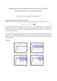
<strong>What</strong> <strong>can</strong> <strong>be</strong> <strong>learned</strong> <strong>about</strong> <strong>carbon</strong> <strong>cycle</strong> <strong>climate</strong> <strong>feedbacks</strong> <strong>from</strong> <strong>the</strong><br />
CO 2 airborne fraction?<br />
M. Gloor 1 , J. L. Sarmiento 2 , and N. Gru<strong>be</strong>r 3<br />
1 The School of Geography, University of Leeds, Leeds, LS2 9JT, UK<br />
2 Atmospheric and Oceanic Sciences Department, Princeton University, 300 Forrestal Road, Sayre Hall, Princeton,<br />
NJ 08544, USA<br />
3 Institute of Biogeochemistry and Pollutant Dynamics, ETH Zürich, Universitätsstr. 16, 8092 Zürich, Switzerland<br />
Received: 22 March 2010 – Published in Atmos. Chem. Phys. Discuss.: 8 April 2010<br />
Revised: 18 June 2010 – Accepted: 21 July 2010 – Published: 20 August 2010<br />
Abstract. The ratio of CO 2 accumulating in <strong>the</strong> atmosphere<br />
to <strong>the</strong> CO 2 flux into <strong>the</strong> atmosphere due to human activity,<br />
<strong>the</strong> airborne fraction AF, is central to predict changes<br />
in earth’s surface temperature due to greenhouse gas induced<br />
warming. This ratio has remained remarkably constant in <strong>the</strong><br />
past five decades, but recent studies have reported an apparent<br />
increasing trend and interpreted it as an indication for a<br />
decrease in <strong>the</strong> efficiency of <strong>the</strong> combined sinks by <strong>the</strong> ocean<br />
and terrestrial biosphere. We investigate here whe<strong>the</strong>r this<br />
interpretation is correct by analyzing <strong>the</strong> processes that control<br />
long-term trends and decadal-scale variations in <strong>the</strong> AF.<br />
To this end, we use simplified linear models for describing<br />
<strong>the</strong> time evolution of an atmospheric CO 2 perturbation. We<br />
find firstly that <strong>the</strong> spin-up time of <strong>the</strong> system for <strong>the</strong> AF to<br />
converge to a constant value is on <strong>the</strong> order of 200–300 years<br />
and differs depending on whe<strong>the</strong>r exponentially increasing<br />
fossil fuel emissions only or <strong>the</strong> sum of fossil fuel and land<br />
use emissions are used. We find secondly that <strong>the</strong> primary<br />
control on <strong>the</strong> decadal time-scale variations of <strong>the</strong> AF is variations<br />
in <strong>the</strong> relative growth rate of <strong>the</strong> total anthropogenic<br />
CO 2 emissions. Changes in sink efficiencies tend to leave a<br />
smaller imprint. Therefore, <strong>be</strong>fore interpreting trends in <strong>the</strong><br />
AF as an indication of weakening <strong>carbon</strong> sink efficiency, it<br />
is necessary to account for trends and variations in AF stemming<br />
<strong>from</strong> anthropogenic emissions and o<strong>the</strong>r extrinsic forcing<br />
events, such as vol<strong>can</strong>ic eruptions. Using atmospheric<br />
CO 2 data and emission estimates for <strong>the</strong> period 1959 through<br />
2006, and our simple predictive models for <strong>the</strong> AF, we find<br />
that likely omissions in <strong>the</strong> reported emissions <strong>from</strong> land use<br />
change and extrinsic forcing events are sufficient to explain<br />
Correspondence to: M. Gloor<br />
(eugloor@googlemail.com)<br />
<strong>the</strong> observed long-term trend in AF. Therefore, claims for a<br />
decreasing long-term trend in <strong>the</strong> <strong>carbon</strong> sink efficiency over<br />
<strong>the</strong> last few decades are currently not supported by atmospheric<br />
CO 2 data and anthropogenic emissions estimates.<br />
1 Introduction<br />
Central for predicting future temperatures of <strong>the</strong> Earth’s surface<br />
is how much and for how long <strong>carbon</strong> dioxide <strong>from</strong><br />
fossil fuel emissions and land use change stays in <strong>the</strong> atmosphere,<br />
and how much gets removed by <strong>the</strong> <strong>carbon</strong> sinks on<br />
land and in <strong>the</strong> ocean (e.g. Solomon et al., 2009). A straightforward<br />
measure of this redistribution is <strong>the</strong> ratio <strong>be</strong>tween<br />
<strong>the</strong> increase rate in atmospheric CO 2 and <strong>the</strong> CO 2 emitted<br />
to <strong>the</strong> atmosphere by human activity (fossil fuel burning<br />
and land use change). Keeling (1973) termed this quantity<br />
<strong>the</strong> “airborne fraction” (AF) and it was investigated in<br />
many subsequent studies (e.g. Bacastow and Keeling, 1979;<br />
Oeschger and Heimann, 1983; Enting, 1986). Because of <strong>the</strong><br />
large uncertainties in land fluxes, <strong>the</strong>se early studies could<br />
estimate <strong>the</strong> value of AF only to within a wide range <strong>from</strong><br />
0.38 to 0.78 (Oeschger and Heimann, 1983). Recently several<br />
studies have extended <strong>the</strong> estimation of AF over <strong>the</strong> last<br />
two decades, with a suggestion of a positive trend in AF<br />
(Canadell et al., 2007; Raupach et al., 2008; Le Quéré et al.,<br />
2009). Moreover, this positive trend has <strong>be</strong>en interpreted as<br />
evidence for a decreasing trend in <strong>the</strong> efficiency of <strong>the</strong> ocean<br />
and land <strong>carbon</strong> sinks. Given <strong>the</strong> model-based projection of<br />
a substantial reduction in <strong>the</strong> sink strength of <strong>the</strong> ocean and<br />
land in <strong>the</strong> future (e.g. by a large-scale dieback of <strong>the</strong> Amazon<br />
old-growth forest, Cox et al., 2000), <strong>the</strong> notion that <strong>the</strong><br />
sinks have already <strong>be</strong>gun to deviate <strong>from</strong> a linear response<br />
Published by Copernicus Publications on <strong>be</strong>half of <strong>the</strong> European Geosciences Union.
7740 M. Gloor et al.: Airborne fraction trends and <strong>carbon</strong> sink efficiency<br />
to <strong>the</strong> atmospheric CO 2 perturbation is a source of substantial<br />
concern. While <strong>the</strong>re remains discussion <strong>about</strong> whe<strong>the</strong>r<br />
this trend in <strong>the</strong> AF is actually statistically signifi<strong>can</strong>t (Knorr,<br />
2009), we focus our discussion here on whe<strong>the</strong>r <strong>the</strong> inferred<br />
conclusion is defensible, i.e. whe<strong>the</strong>r an increasing trend in<br />
<strong>the</strong> AF implies a decreasing efficiency of <strong>the</strong> <strong>carbon</strong> sinks.<br />
Determinants of <strong>the</strong> AF are <strong>the</strong> magnitude and time course<br />
of <strong>the</strong> human induced emissions of CO 2 into <strong>the</strong> atmosphere<br />
and <strong>the</strong> removal of this anthropogenic <strong>carbon</strong> by <strong>the</strong> ocean<br />
and land biosphere. It has <strong>be</strong>en known since <strong>the</strong> early 1970’s,<br />
possibly earlier, that <strong>the</strong> AF will eventually asymptote to a<br />
constant value if (i) <strong>the</strong> CO 2 uptake by <strong>the</strong> oceans and land<br />
ecosystems is linear and (ii) if CO 2 emissions to <strong>the</strong> atmosphere<br />
follow exactly an exponential function (Bacastow and<br />
Keeling, 1979). Thus, given that fossil fuel emissions have<br />
risen approximately exponentially over <strong>the</strong> last 250 years,<br />
and that natural systems tend to respond linearly to small perturbations,<br />
it is natural to inquire whe<strong>the</strong>r time trends in AF<br />
may inform us <strong>about</strong> changes in <strong>the</strong> linear <strong>be</strong>havior of <strong>carbon</strong><br />
uptake by <strong>the</strong> oceans and land ecosystems (Canadell et<br />
al., 2007; Raupach et al., 2008; Le Quéré et al., 2009; Rafelski<br />
et al., 2009). However, closer examination shows that <strong>the</strong><br />
relative growth rate RGR≡ 1 of fossil fuel emissions FF<br />
has varied by more than a factor of two in <strong>the</strong> last 100 years<br />
(e.g. Raupach et al., 2008). In addition, emissions <strong>from</strong> land<br />
use change exhibited an even more varied time course, so<br />
that <strong>the</strong> total emissions only very approximately followed a<br />
single exponential. Fur<strong>the</strong>rmore, trends in AF may <strong>be</strong> an articulation<br />
of an incomplete spin-up of <strong>the</strong> system, so that <strong>the</strong><br />
AF is still changing along its way toward reaching its asymptotic<br />
value. We examine here <strong>the</strong> impact of <strong>the</strong>se deviations<br />
and controls on <strong>the</strong> AF, and what <strong>the</strong> consequences are for<br />
<strong>the</strong> interpretation of <strong>the</strong> AF as an indicator for changes in <strong>the</strong><br />
efficiency of <strong>carbon</strong> sinks, and in turn <strong>the</strong> state of <strong>the</strong> global<br />
<strong>carbon</strong> <strong>cycle</strong>. Our study builds on <strong>the</strong> seminal work of Bacastow<br />
and Keeling (1979) who had stated already 30 years<br />
ago that “The global average airborne fraction will probably<br />
not remain near 56% in <strong>the</strong> future ... <strong>be</strong>cause fossil fuel resources<br />
are finite...”, i.e. that one important control of <strong>the</strong> AF<br />
is <strong>the</strong> growth rate of fossil fuel emissions.<br />
Before proceeding, it is important to recognize that definitions<br />
of <strong>the</strong> AF in <strong>the</strong> literature vary. Studies <strong>from</strong> <strong>the</strong> 1970s<br />
and 1980s defined airborne fraction <strong>from</strong> cumulative <strong>carbon</strong><br />
inventory changes as<br />
AF cum<br />
∫ tf<br />
FF ≡ C(t f)−C(t i )<br />
t i<br />
FF(t)dt<br />
FF dFF<br />
dt<br />
(Keeling, 1973; Bacastow and Keeling, 1979; Enting, 1986)<br />
or alternatively as<br />
AF cum<br />
∫ tf<br />
FF+LU ≡ C(t f )−C(t i )<br />
t i<br />
FF(t)+LU(t)dt<br />
(Oeschger and Heimann, 1983) where C is atmospheric <strong>carbon</strong><br />
dioxide, t i ,t f are <strong>the</strong> <strong>be</strong>ginning and <strong>the</strong> end time of <strong>the</strong><br />
period considered, FF is fossil fuel emissions and LU is <strong>the</strong><br />
flux to <strong>the</strong> atmosphere due to land use change. The more recent<br />
studies define airborne fraction <strong>from</strong> annual or monthly<br />
inventory changes as ei<strong>the</strong>r<br />
AF FF ≡<br />
dC(t)<br />
dC(t)<br />
dt<br />
FF(t) , or AF dt<br />
FF+LU ≡<br />
FF(t)+LU(t)<br />
(Canadell et al., 2007; Raupach et al., 2008; Le Quéré et al.,<br />
2009; Knorr, 2009). We analyze here <strong>the</strong> time-evolution of<br />
<strong>the</strong> AF as defined by <strong>the</strong>se recent studies.<br />
We briefly outline <strong>the</strong> organization of our paper. We start<br />
in Sect. 2 with a characterization of <strong>the</strong> time course of anthropogenic<br />
CO 2 emissions and <strong>carbon</strong> sinks, <strong>the</strong>reby highlighting<br />
that <strong>the</strong>re have <strong>be</strong>en strong variations in <strong>the</strong> relative<br />
growth rate of fossil fuel emissions over <strong>the</strong> last century. In<br />
Sect. 3 we introduce a simple linear model of <strong>the</strong> evolution<br />
of an atmospheric CO 2 perturbation, <strong>the</strong>reby also clarifying<br />
<strong>the</strong> meaning of “sink efficiency”. In Sect. 4 we explore how<br />
<strong>the</strong> time course of <strong>the</strong> anthropogenic emissions controls variations<br />
in <strong>the</strong> AF, using a predictive equation implied by our<br />
simple model. We demonstrate that (i) for an atmospheric<br />
CO 2 perturbation which is not following an exact exponential<br />
function, <strong>the</strong>re is an adjustment time for <strong>the</strong> AF to converge<br />
to its constant asymptotic value, which is on <strong>the</strong> order<br />
of centuries, and that (ii) variations in <strong>the</strong> relative growth<br />
rate of <strong>the</strong> anthropogenic emissions are a major control on<br />
variations of <strong>the</strong> AF. Therefore, in order to unravel trends in<br />
<strong>the</strong> AF caused by trends in <strong>carbon</strong> sink efficiency or extrinsic<br />
non-anthropogenic events, like vol<strong>can</strong>ic eruptions, signatures<br />
due to incomplete “spin-up” and fossil fuel growth<br />
rate variations, need first to <strong>be</strong> removed <strong>from</strong> <strong>the</strong> observed<br />
AF. We <strong>can</strong> achieve this using our predictive equation for<br />
<strong>the</strong> AF (Sect. 5). We <strong>the</strong>n examine <strong>the</strong> remaining signal for<br />
trends not explained by known extrinsic non-anthropogenic<br />
forcings or omissions in anthropogenic fluxes, to conclude<br />
whe<strong>the</strong>r <strong>the</strong>re is indeed evidence for trends in <strong>the</strong> <strong>carbon</strong><br />
sink efficiency trends in <strong>the</strong> observed AF record (Sect. 6).<br />
This terminates our main analysis. Section 7 in addition explores<br />
<strong>the</strong> signal to noise ratio of AF trends caused by sink<br />
efficiency trends, and finally we discuss and conclude.<br />
2 Anthropogenic <strong>carbon</strong> emissions and <strong>carbon</strong> sinks<br />
The main driver of <strong>the</strong> rapid increase in atmospheric CO 2<br />
is fossil fuel emissions, which are estimated <strong>from</strong> national<br />
energy statistics with an uncertainty of 6%–10% (90% confidence<br />
interval) (Marland, 2006, updated by Boden et al.,<br />
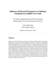
2009; Marland, 2008). A logarithmic representation (Fig. 1a)<br />
reveals that fossil fuel emissions have increased roughly exponentially,<br />
with <strong>the</strong> time-scale of relative change, <strong>the</strong> inverse<br />
of <strong>the</strong> relative growth rate, varying roughly <strong>be</strong>tween<br />
∼20 and 150 years (Fig. 1b).<br />
Atmos. Chem. Phys., 10, 7739–7751, 2010<br />
www.atmos-chem-phys.net/10/7739/2010/
M. Gloor et al.: Airborne fraction trends and <strong>carbon</strong> sink efficiency 7741<br />
FF (PgC yr -1 )<br />
10<br />
1<br />
0.1<br />
a<br />
fossil fuel (FF)<br />
τ f<br />
=(df/dt/f) -1 (yr)<br />
160<br />
120<br />
80<br />
40<br />
0<br />
b<br />
τ of fossil fuel (FF)<br />
WW1 WW2 oil crisis<br />
2000<br />
end of<br />
USSR<br />
LU (PgC yr -1 )<br />
2<br />
1.5<br />
1<br />
0.5<br />
c<br />
land-use change (LU)<br />
2000<br />
AF (−)<br />
-1<br />
RGR = τ f<br />
(yr -1 )<br />
0.08<br />
0.06<br />
0.04<br />
0.02<br />
0<br />
−0.02<br />
1<br />
0.8<br />
0.6<br />
0.4<br />
d<br />
e<br />
RGR fossil fuel & land use (FF+LU)<br />
modeled AF (FF only)<br />
modeled AF<br />
(FF+LU)<br />
RGR fossil fuel (FF)<br />
observed AF (FF only)<br />
observed AF<br />
(FF+LU)<br />
2000<br />
2000<br />
0.2<br />
1750 1800 1850 1900 1950<br />
2000<br />
Fig. 1. (a) Fossil fuel emissions estimated by Marland (2006), (b) time scale τ f of relative rate of change of FF, (c) <strong>carbon</strong> flux to <strong>the</strong><br />
atmosphere due to land use change estimated by Houghton et al. (2007), (d) relative growth rate of f =FF and f =FF+LU respectively, and<br />
(e) model predicted and observed AF FF and AF FF+LU .<br />
The time-scale τ f of relative change of an anthropogenic<br />
flux f to <strong>the</strong> atmosphere is defined as <strong>the</strong> inverse of its logarithmic<br />
derivative:<br />
τ f ≡ ( 1 f<br />
df<br />
dt )−1 ≃ ( 1 f<br />
f t )−1<br />
with f ≡ f (t +t) − f (t) and t = 1 year. The timecourse<br />
of τ f permits to identify periods with different fossil<br />
fuel emissions growth rates particularly well.<br />
Variations in <strong>the</strong> time-scale of relative change of fossil fuel<br />
emissions, τ f , are mainly due to economic <strong>cycle</strong>s and wars.<br />
Thus <strong>the</strong>re was an approximately 80 year period <strong>from</strong> around<br />
1830 to 1910 (approximately <strong>the</strong> start date of World War<br />
one (WW1)) with a roughly constant τ FF ≡ (<br />
FF 1 dFF<br />
dt<br />
) −1 ≃<br />
(<br />
FF 1 FF<br />
t<br />
) −1 of ∼20 years (equivalent to a relative growth rate<br />
of 5% per year, Fig. 1d). The WW1, post WW1 and great depression<br />
period saw less growth, with both positive and negative<br />
time-scales resulting in a substantially longer mean τ FF .<br />
After WW2 (starting around 1948) <strong>the</strong>re is again fast growth,<br />
paralleling <strong>the</strong> recovery of industrial countries’ economies,<br />
until <strong>the</strong> early 1970s with τ FF of ∼20 years. From <strong>the</strong> early<br />
1970s until approximately 1999 τ FF increased again to ∼80<br />
years (relative growth rate of ∼1.3% yr −1 ). Growth returned<br />
close to <strong>the</strong> 1830 to 1910 and post WW2 values starting<br />
around 2001.<br />
www.atmos-chem-phys.net/10/7739/2010/ Atmos. Chem. Phys., 10, 7739–7751, 2010
7742 M. Gloor et al.: Airborne fraction trends and <strong>carbon</strong> sink efficiency<br />
The second cause of <strong>the</strong> rise in atmospheric <strong>carbon</strong>, and at<br />
<strong>the</strong> same time <strong>the</strong> least well constrained positive component<br />
of <strong>the</strong> atmospheric <strong>carbon</strong> budget, is <strong>carbon</strong> fluxes released<br />
<strong>from</strong> land to <strong>the</strong> atmosphere due to land use change (for example<br />
rainforest to pasture conversion in <strong>the</strong> tropics, or peat<br />
burning during 1997/98 in Indonesia due to conversion of<br />
swamp forests to rice paddies at a large spatial scale, Page et<br />
al., 2002). Estimates of Houghton et al. (2007) indicate that<br />
this term has also risen in time, but at a considerably smaller<br />
rate than fossil fuel emissions (Fig. 1c). The uncertainty in<br />
fluxes associated with land use change is large, on <strong>the</strong> order<br />
of 40–100%, as revealed by <strong>the</strong> range of published estimates<br />
(e.g. Grainger, 2008; Houghton et al., 2007; DeFries et al.,<br />
2002; Achard et al., 2002).<br />
The atmospheric CO 2 accumulation rate is well constrained<br />
by atmospheric concentration records (Keeling,<br />
1960; E<strong>the</strong>ridge et al., 1996). Estimates of ocean uptake of<br />
anthropogenic <strong>carbon</strong> based on various methods have also<br />
converged over recent years to 2.2±0.2 PgC yr −1 for a nominal<br />
period of ∼1995–2000 (Sabine et al., 2004; Sweeney et<br />
al., 2007; Sarmiento et al., 2010; Gru<strong>be</strong>r et al., 2009; Khatiwala<br />
et al., 2009). The net land sink, <strong>the</strong> sum of <strong>the</strong> land sink<br />
and <strong>the</strong> CO 2 flux to <strong>the</strong> atmosphere due to land use change,<br />
<strong>can</strong> <strong>the</strong>n <strong>be</strong> calculated as <strong>the</strong> difference <strong>be</strong>tween fossil fuel<br />
emissions, <strong>the</strong> atmospheric CO 2 accumulation rate and ocean<br />
uptake. The implied net land sink stayed roughly constant<br />
with a mean value of nearly zero <strong>from</strong> <strong>the</strong> 1930s to 1990 and<br />
<strong>the</strong>n increased to a magnitude of approximately 1 PgC yr −1<br />
for <strong>the</strong> 1990s and early 2000s (e.g., Sarmiento et al., 2010).<br />
3 A simple <strong>carbon</strong> <strong>cycle</strong> model<br />
We investigate <strong>the</strong> processes controlling time-variations of<br />
<strong>the</strong> airborne fraction with simple linear models of <strong>the</strong> global<br />
perturbation of <strong>the</strong> <strong>carbon</strong> <strong>cycle</strong>. This is justified on two<br />
grounds. First any claim of a possible non-linear <strong>be</strong>haviour<br />
of <strong>the</strong> system must <strong>be</strong> shown to differ <strong>from</strong> <strong>the</strong> prediction of<br />
such linear models. Secondly, <strong>the</strong> concept of an efficiency,<br />
like <strong>the</strong> efficiency of a heat engine, is inherently linear. This<br />
is <strong>be</strong>cause an efficiency is defined as <strong>the</strong> ratio <strong>be</strong>tween <strong>the</strong><br />
magnitude of an effect and <strong>the</strong> magnitude of its cause. In<br />
our case <strong>the</strong> cause is <strong>the</strong> increase in atmospheric CO 2 due to<br />
human activity and <strong>the</strong> effect is <strong>the</strong> <strong>carbon</strong> flux <strong>from</strong> <strong>the</strong> atmosphere<br />
to <strong>the</strong> ocean and land <strong>carbon</strong> pools. If we treat <strong>the</strong><br />
ocean and land each as a single pool of <strong>carbon</strong> with a constant<br />
sink efficiency, <strong>the</strong>n <strong>the</strong> fluxes <strong>from</strong> <strong>the</strong> atmosphere to<br />
<strong>the</strong> oceans and to <strong>the</strong> land F at→oc and F at→ld , are given by<br />
F at→oc = C<br />
τ oc<br />
, F at→ld = C<br />
τ ld<br />
. (1)<br />
Here C ≡ C(t) − C(1765) is <strong>the</strong> anthropogenic perturbation<br />
of atmospheric <strong>carbon</strong> dioxide, and τ oc and τ ld are constants.<br />
In this context a weakening/streng<strong>the</strong>ning of <strong>the</strong> sinks<br />
means that τ oc and/or, τ ld are increasing/decreasing in time.<br />
With <strong>the</strong> flux parameterization given by Eq. (1), <strong>the</strong> time<br />
evolution for C implied by <strong>the</strong> atmospheric CO 2 mass balance<br />
is determined by<br />
dC<br />
dt<br />
= f (t)−F at→oc −F at→ld<br />
= f (t)−( 1<br />
τ oc<br />
+ 1<br />
τ ld<br />
)C = f (t)− C<br />
τ s<br />
. (2)<br />
Here t is time, <strong>the</strong> subscript s stands for “system”,<br />
1<br />
≡ 1 + 1<br />
τ s τ oc τ ld<br />
is <strong>the</strong> proportionality constant <strong>be</strong>tween <strong>the</strong> atmospheric CO 2<br />
perturbation and <strong>the</strong> total C flux out of <strong>the</strong> atmosphere, and<br />
f (t) is <strong>the</strong> anthropogenic CO 2 flux into <strong>the</strong> atmosphere,<br />
which we <strong>can</strong> view as <strong>the</strong> forcing of <strong>the</strong> system. For our<br />
problem f is mostly FF+LU although we will also consider<br />
<strong>the</strong> case of f =FF alone.<br />
It is necessary to consider to what extent <strong>the</strong> assumption of<br />
a linear relationship <strong>be</strong>tween <strong>the</strong> flux out of <strong>the</strong> atmosphere<br />
and <strong>the</strong> anthropogenic atmospheric CO 2 perturbation is justified<br />
based on our understanding of <strong>the</strong> dominant processes.<br />
In <strong>the</strong> case of ocean <strong>carbon</strong> uptake, this assumption is well<br />
underpinned, <strong>be</strong>cause <strong>the</strong> driving force for <strong>the</strong> uptake is <strong>the</strong><br />
air-sea CO 2 disequilibrium. In addition, <strong>the</strong> rate-limiting step<br />
of <strong>the</strong> oceanic uptake, <strong>the</strong> transport of <strong>the</strong> anthropogenic CO 2<br />
into <strong>the</strong> ocean’s interior, is a linear process (e.g. Sarmiento et<br />
al., 1992; Maier-Reimer and Hasselmann, 1987). The linear<br />
scaling of <strong>the</strong> ocean uptake with <strong>the</strong> perturbation in atmospheric<br />
CO 2 is supported by 3-D ocean model simulations<br />
(e.g., Sarmiento and Le Quéré, 1996), although such simulations<br />
also show a strong deviation <strong>from</strong> linearity once atmospheric<br />
CO 2 has risen to values where <strong>the</strong> surface ocean<br />
buffer factor <strong>be</strong>gins to change rapidly (Sarmiento and Le<br />
Quéré, 1996). Using <strong>the</strong> model-based scaling used by Gloor<br />
et al. (2003) and Mikaloff-Fletcher et al. (2006) and <strong>the</strong> anthropogenic<br />
ocean <strong>carbon</strong> inventory estimated <strong>from</strong> oceans<br />
surveys for 1995 (Sabine et al., 2004), we obtain an estimate<br />
of τ oc ≃ 81.4 yr (Appendix C).<br />
For uptake by <strong>the</strong> land vegetation it is less clear whe<strong>the</strong>r<br />
<strong>the</strong> linearity concept applies. This is <strong>be</strong>cause uptake by land,<br />
unlike <strong>the</strong> oceans, is tied to processes such as productivity<br />
and <strong>the</strong> status of <strong>the</strong> land vegetation, some of which may<br />
<strong>be</strong> related to <strong>the</strong> atmospheric CO 2 perturbation (specifically<br />
CO 2 uptake during photosyn<strong>the</strong>sis), while o<strong>the</strong>rs like nutrient<br />
and micronutrient availability, plant and soil respiration,<br />
vegetation population dynamics, and land use change are<br />
not. Even if <strong>the</strong>re were a productivity increase due to CO 2<br />
“fertilization”, it would likely <strong>be</strong> a linear response only during<br />
a limited period of time until land vegetation reaches a<br />
new steady state balance <strong>be</strong>tween growth and mortality. The<br />
linear response assumption of <strong>the</strong> land vegetation thus confounds<br />
many processes and time-scales (e.g., Lloyd, 1999).<br />
Despite <strong>the</strong>se obvious caveats, we never<strong>the</strong>less descri<strong>be</strong>d in a<br />
Atmos. Chem. Phys., 10, 7739–7751, 2010<br />
www.atmos-chem-phys.net/10/7739/2010/
M. Gloor et al.: Airborne fraction trends and <strong>carbon</strong> sink efficiency 7743<br />
first step <strong>the</strong> land uptake as <strong>be</strong>ing linearly related to <strong>the</strong> atmospheric<br />
perturbation with a single time-scale, with <strong>the</strong> intention<br />
to generalize <strong>the</strong> description if <strong>the</strong> data were to contain<br />
sufficient information.<br />
One could question <strong>the</strong> realism of our simple model on<br />
<strong>the</strong> grounds that <strong>the</strong> model treats both <strong>the</strong> oceans and <strong>the</strong><br />
land vegetation as just one integral pool, while for both, several<br />
pools with different characteristic exchange time scales<br />
is more realistic. We tested this for <strong>the</strong> ocean and it turns<br />
out that inclusion of multiple ocean pools does not alter our<br />
conclusions for <strong>the</strong> reason explained in Sect. 5.<br />
4 Airborne fraction for idealized cases<br />
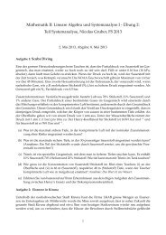
To get a general sense of <strong>the</strong> implications of our simple<br />
model (Eq. 2) for <strong>the</strong> time-course of AF, we have calculated<br />
AF for three idealized forcing functions f (t): (i) exponential<br />
forcing f (t) = f e t/τ f with a single characteristic time-scale<br />
τ f (or equivalently relative growth rate 1/τ f ); <strong>the</strong> subscript<br />
f refers to “forcing”, (ii) <strong>the</strong> sum of an exponential function<br />
and a constant, and (iii) <strong>the</strong> sum of several exponential<br />
functions with different characteristic time-scales or relative<br />
growth rates (Appendix A and Fig. 2). The first case is an<br />
idealization of forcing <strong>the</strong> atmosphere with fossil fuel burning<br />
CO 2 alone, while <strong>the</strong> latter two cases mimic forcing of<br />
<strong>the</strong> atmosphere with <strong>the</strong> sum of fossil fuel emissions and land<br />
use change emissions.<br />
As shown previously (e.g. Bacastow and Keeling, 1979),<br />
AF is constant for a purely exponential forcing function (Appendix<br />
A and Fig. 2). For <strong>the</strong> forcing functions differing <strong>from</strong><br />
an exact exponential function, AF converges to an asymptotic<br />
value after some spin up time. The asymptotic value of AF<br />
is <strong>the</strong> same for <strong>the</strong> three forcing functions and is given by<br />
AF(∞) = 1<br />
1+ τ f<br />
τ s<br />
.<br />
It is thus controlled by <strong>the</strong> ratio <strong>be</strong>tween <strong>the</strong> forcing timescale<br />
and <strong>the</strong> system response time-scale. If <strong>the</strong> forcing is<br />
not exactly exponential, <strong>the</strong>n <strong>the</strong> time-scale for convergence<br />
is roughly on <strong>the</strong> order of 200–300 years (Fig. 2), depending<br />
on <strong>the</strong> exact functional form of <strong>the</strong> forcing. For <strong>the</strong> case<br />
of forcing by <strong>the</strong> sum of several exponentials it is <strong>the</strong> τ f of<br />
<strong>the</strong> fastest growing exponential function that determines <strong>the</strong><br />
asymptotic value of AF (see last equation in Appendix A).<br />
An intuitive explanation for <strong>the</strong> existence of a spin-up period<br />
is as follows. The constancy of AF for a purely exponential<br />
forcing reflects <strong>the</strong> balance <strong>be</strong>tween two exponential processes,<br />
exponential damping of <strong>the</strong> atmospheric perturbation<br />
via <strong>carbon</strong> sinks and exponential forcing (Appendix B). If <strong>the</strong><br />
forcing deviates <strong>from</strong> a pure exponential function, <strong>the</strong>re will<br />
<strong>be</strong> a spin up period until <strong>the</strong> exponential component of <strong>the</strong><br />
forcing dominates over o<strong>the</strong>r slower growing components of<br />
<strong>the</strong> forcing. An implication of <strong>the</strong> existence of a spin-up period<br />
is that we expect observed AF FF+LU to converge towards<br />
AF FF <strong>from</strong> lower values. This is <strong>be</strong>cause fossil fuel emissions<br />
rise approximately exponentially but land use change<br />
emissions rise more slowly and thus <strong>the</strong>ir sum will not equal<br />
an exact exponential function (Sect. 2 and Fig. 1a and c).<br />
5 Predicted and observed airborne fraction<br />
Instead of idealized cases we now predict <strong>the</strong> time-course<br />
of AF using <strong>the</strong> observed FF and LU emissions. For this<br />
purpose we use <strong>the</strong> differential equation for AF implied by<br />
our model Eq. (2)<br />
dAF<br />
dt<br />
= ( 1 df<br />
f dt + 1 dτ s<br />
τ s dt )−( 1 + 1 df<br />
τ s f dt + 1 dτ s<br />
)AF (3)<br />
τ s dt<br />
df<br />
dt + τ 1 dτ s<br />
s<br />
derived in Appendix B. In order to interpret this equation it<br />
is helpful to notice that it is quite similar to Eq. (2). The<br />
analogue of C is AF, <strong>the</strong> analogue of <strong>the</strong> “forcing” flux to<br />
<strong>the</strong> atmosphere f (t) is<br />
f<br />
1 df<br />
dt + τ 1 dτ s<br />
s dt<br />
, and <strong>the</strong> analogue of <strong>the</strong><br />
exponential damping term − C<br />
τ s<br />
is −(<br />
τ 1 s<br />
+<br />
f<br />
1 df<br />
dt + τ 1 dτ s<br />
s dt )AF.<br />
Growth of AF is thus largely dictated by <strong>the</strong> relative growth<br />
rate RGR=<br />
f<br />
1 df<br />
dt<br />
of f (instead of f itself;<br />
f<br />
1 df<br />
dt<br />
≫<br />
τ 1 dτ s<br />
s dt<br />
unless<br />
<strong>the</strong>re is a very strong feedback), and AF is damped towards<br />
zero at a rate<br />
τ 1 s<br />
+<br />
f<br />
1 dt<br />
(instead of<br />
τ 1 s<br />
).<br />
To predict <strong>the</strong> variations in AF according to our simple<br />
model, we integrate <strong>the</strong> equation numerically assuming a<br />
constant sink efficiency, i.e. τ s = const. We choose a value<br />
for τ s such that <strong>the</strong> mean observed and predicted AF are equal<br />
over <strong>the</strong> period 1959–2006 using least squares, which results<br />
in τ s =42 years for AF FF and τ s =37.5 years for AF FF+LU . Besides<br />
using <strong>the</strong> requirement for agreement of <strong>the</strong> mean AF<br />
over <strong>the</strong> period <strong>from</strong> 1959 to 2006 to estimate τ s , we may also<br />
determine τ s <strong>from</strong> <strong>the</strong> mass conservation requirement that<br />
predicted and observed increase in atmospheric CO 2 agree.<br />
The two estimates agree well. The predicted variations in<br />
AF based on <strong>the</strong> fossil fuel time-series estimated by Marland<br />
(2006) alone, as well as <strong>the</strong> sum of <strong>the</strong> fossil fuel and land<br />
use time-series, used as forcing, are shown in Figs. 1e and<br />
3a.<br />
In order to assess <strong>the</strong> importance of restricting ourselves<br />
to a single ocean and land pool description for our results,<br />
we repeated this calculation using a more generalized form<br />
of <strong>the</strong> predictive equation for AF. The generalized form is<br />
based on a linear multi-pool representation of <strong>the</strong> ocean, or<br />
equivalently a sum of impulse response functions (Greens<br />
functions) with characteristic time-scales of τ 0 = ∞,τ 1 =<br />
433.3 yr, τ 2 = 83.9 yr, τ 3 = 11.2 yr, and τ 4 = 0.8 yr (see Appendices<br />
B and D). The predicted AF is nearly <strong>the</strong> same as<br />
AF predicted by <strong>the</strong> simple single pool model, confirming<br />
that <strong>the</strong> simple model suffices to analyse <strong>the</strong> controls on <strong>the</strong><br />
AF during <strong>the</strong> 1959–2006 period. The reason is that ocean<br />
<strong>carbon</strong> uptake during this period is primarily governed by<br />
one Green’s function, <strong>the</strong> one associated with τ 2 = 83.9 yr<br />
(which is close to τ oc ).<br />
www.atmos-chem-phys.net/10/7739/2010/ Atmos. Chem. Phys., 10, 7739–7751, 2010
7744 M. Gloor et al.: Airborne fraction trends and <strong>carbon</strong> sink efficiency<br />
0.8<br />
0.7<br />
0.6<br />
f(t)=fe t/τ f<br />
τ f<br />
/τ s<br />
=20/45=0.444...<br />
τ f<br />
/τ s<br />
=40/45=0.888...<br />
Airborne fraction (−)<br />
0.5<br />
0.4<br />
0.3<br />
f(t)=fe t/τ f+0.1<br />
0.2<br />
f=FF 0<br />
e t/τ f+LU 0<br />
e t/τ LU, τ LU<br />
=110<br />
0.1<br />
τ f<br />
/τ s<br />
=20/4.5=4.444...<br />
0<br />
−200 −150 −100 −50 0 50 100 150 200 250 300<br />
Year<br />
Fig. 2. Predicted air-borne fraction for a range of forcings including purely exponential forcing f (t) = f e t/τ f (blue), mixed exponential and<br />
constant forcing f (t) Fig. = f2. e t/τ f<br />
Predicted +f 0 with air-borne f 0 = fraction 0.1 (black), for a range and forcing of forcings byincluding <strong>the</strong> sum of purely two exponential forcing functions, f (t) = f f(t) e t/τ = f f e t/τ f +f LU e t/τ LU<br />
(red).<br />
(blue), mixed exponential and constant forcing f (t) = f e t/τ f + f 0 with f 0 = 0.1 (black), and forcing by <strong>the</strong><br />
sum of two exponential functions, f (t) = f e t/τ f +f LU e t/τ LU (red).<br />
The model computed AF FF and AF FF+LU agree remarkably<br />
well with <strong>the</strong> observed ones, calculated <strong>from</strong> tinctly different phases: 1958–1973 fast growth, small<br />
The forcing during <strong>the</strong> period 1959–2006 has three dis-<br />
160<br />
atmospheric concentration<br />
If <strong>the</strong> forcing<br />
data<br />
is not<br />
(<strong>from</strong><br />
exactly<br />
Mauna<br />
exponential,<br />
Loa)<br />
<strong>the</strong>n<br />
and<br />
<strong>the</strong> time-scale<br />
τ<br />
for convergence is roughly on <strong>the</strong> order<br />
f ∼20 yr; 1973–1999: slow growth, large τ f ∼30–150 years;<br />
anthropogenic emissions. of 200-300The years numerator (Fig. 2), depending of <strong>the</strong> observed on <strong>the</strong> exact functional 2000–2006: form of fast <strong>the</strong>growth, forcing. small τ f ∼25 years, (Fig. 1b). We<br />
AF FF and AF FF+LU An were intuitive calculated explanation usingfor <strong>the</strong> <strong>the</strong>atmospheric<br />
existence of a spin-up thus period expectis<strong>the</strong> as follows. predicted TheAF constancy to decrease of AFduring <strong>the</strong> 1973–<br />
rate of change, dC/dt, taken <strong>from</strong> <strong>the</strong> monthly mean 1999 period and <strong>the</strong>n to increase again with some lag. This<br />
for a purely exponential forcing reflects <strong>the</strong> balance <strong>be</strong>tween two exponential processes, exponential<br />
records <strong>from</strong> NOAA ESRL (co2 mm mlo.2009.txt obtained is indeed what we find (Figs. 1e, 3a). The same signature<br />
in Novem<strong>be</strong>r 2009 damping <strong>from</strong>offtp://ftp.cmdl.noaa.gov/ccg/co2/<br />
<strong>the</strong> atmospheric perturbation via <strong>carbon</strong>seems sinks and to <strong>be</strong> exponential present in forcing <strong>the</strong> observations (appendix B). as If well, although it<br />
trends/, Tans, 165 2009a). <strong>the</strong> forcing From <strong>the</strong>se deviates monthly <strong>from</strong> a pure data exponential we first calculated<br />
annual means nential centered component on 31 of <strong>the</strong> Decem<strong>be</strong>r/1 forcing dominates January, over o<strong>the</strong>r thisslower modelgrowing <strong>the</strong>re iscomponents indeed a tight of <strong>the</strong> relation forcing. <strong>be</strong>tween AF and <strong>the</strong><br />
function, tends <strong>the</strong>re towill <strong>be</strong> masked <strong>be</strong> a spinby up<strong>the</strong> period larger until variability. <strong>the</strong> expo- Fur<strong>the</strong>rmore for<br />
<strong>from</strong> which we estimated <strong>the</strong> time derivative by differencing. relative growth rate RGR of anthropogenic emissions (compare<br />
Fig. 1d and e).<br />
An implication of <strong>the</strong> existence of a spin-up period is that we expect observed AF F F +LU to convergeestimates<br />
towards AF are F F annually <strong>from</strong> lower resolved. values. Our This is <strong>be</strong>cause<br />
We estimated <strong>the</strong> dC/dt <strong>from</strong> annual means, <strong>be</strong>cause <strong>the</strong> anthropogenic<br />
emissions As mentioned<br />
fossil fuel emissions<br />
earlier on,<br />
rise<br />
<strong>be</strong>cause<br />
approximately<br />
<strong>the</strong> forcing used to calculate<br />
slowly AF FF+LU and thusis<strong>the</strong>ir approximately sum will not<strong>the</strong> equal sumanof an exponential<br />
conclusions are not exponentially sensitive tobut thisland choice. use change emissions rise more<br />
Observed 170 AF FF exact and exponential AF FF+LU records function (Figs. (section1e, 2). 3a) exhibit<br />
large inter-annual variability, which is missing in <strong>the</strong> we expect AF FF+LU (red dashed line) to <strong>be</strong> lower than AF FF<br />
function, FF, and a less strongly increasing function, LU,<br />
AF FF and AF FF+LU predicted by <strong>the</strong> linear model. This is (blue solid line) and to slope more upwards than AF FF , eventually<br />
converging towards AF FF . This is indeed what is ob-<br />
<strong>be</strong>cause our model 5 isPredicted forced solely and observed by <strong>carbon</strong> airborne fluxesfraction<br />
<strong>from</strong><br />
fossil fuel and land use change, thus variations due to nonanthropogenic<br />
forcings, Insteadlike of vol<strong>can</strong>ic idealized cases eruptions we now or <strong>climate</strong> predict os-<br />
<strong>the</strong> time-course of AF using <strong>the</strong> observed F F and LU<br />
served and predicted (Fig. 1e).<br />
cillations, are not captured. emissions. The For large this purpose inter-annual we use variations <strong>the</strong> differential equation for AF implied by our model equation<br />
in observed air-borne fraction are largely due to inter-annual<br />
variability in <strong>the</strong> rate of change of atmospheric CO 2 , dC<br />
dt , an<br />
6 Causes for trends in observed airborne fraction<br />
observation known since <strong>the</strong> 1970s to <strong>be</strong> associated with El 8<br />
Given <strong>the</strong> variation in AF FF and AF FF+LU due to variations<br />
Niño/La Niña and post vol<strong>can</strong>ic periods (Agung, El Chichon, in forcing (Figs. 1e, 3a), particularly in fossil fuel emissions,<br />
and <strong>the</strong> considerable time it takes for AF to converge<br />
Pinatubo; Bacastow, 1976).<br />
to its asymptotic value, is <strong>the</strong>re none<strong>the</strong>less a possibility to<br />
test whe<strong>the</strong>r <strong>the</strong>re are trends in sink efficiency <strong>from</strong> <strong>the</strong> time<br />
course in AF? If our differential equation for AF based on <strong>the</strong><br />
Atmos. Chem. Phys., 10, 7739–7751, 2010<br />
www.atmos-chem-phys.net/10/7739/2010/
M. Gloor et al.: Airborne fraction trends and <strong>carbon</strong> sink efficiency 7745<br />
0.8<br />
a<br />
modeled AF (FF + LU)<br />
modeled AF (FF + LU + ( ∆f + ∆s))<br />
0.6<br />
AF (−)<br />
0.4<br />
0.2<br />
0.0<br />
observed AF<br />
RGR = τ f<br />
-1<br />
(yr -1 )<br />
∆f + ∆s (PgC yr -1 )<br />
0.08<br />
0.06<br />
0.04<br />
0.02<br />
0<br />
−0.02<br />
2<br />
1<br />
0<br />
−1<br />
−2<br />
b<br />
RGR fossil fuel & land use (FF+LU)<br />
c<br />
Agung<br />
1963-65<br />
RGR fossil fuel (FF)<br />
1991-93<br />
Pinatubo<br />
1998<br />
Indonesia Peat<br />
burning<br />
?<br />
2002-03<br />
2010<br />
2010<br />
AF obs<br />
- AF pred<br />
0.5<br />
0<br />
−0.5<br />
d<br />
residual AF (FF + LU)<br />
residual AF (FF + LU + ( ∆f + ∆s))<br />
2010<br />
C pred<br />
- C obs<br />
(ppm)<br />
2<br />
1<br />
0<br />
−1<br />
−2<br />
e<br />
1955 1960 1965 1970 1975 1980 1985 1990 1995 2000 2005 2010<br />
2010<br />
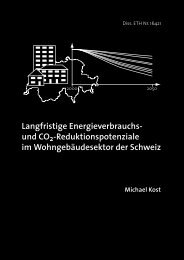
Fig. 3. Time-series <strong>from</strong> 1955 through 2010: (a) model predicted and observed AF FF+LU . Also shown is <strong>the</strong> model-predicted AF after<br />
<strong>the</strong> addition of <strong>the</strong> Fig. “corrections” 3. Time-series shown <strong>from</strong>in 1955 (c), (b) through relative 2010: growth (a) Model rate ofpredicted f =FF and andf observed =FF+LU, AF respectively. F F +LU . Also Shown shown areis<strong>the</strong> annual values<br />
(symbols) and after<br />
<strong>the</strong> modelfiltering<br />
predicted<br />
it with a<br />
AF<br />
low-pass<br />
after <strong>the</strong><br />
filter<br />
addition<br />
(11 year<br />
of<br />
running<br />
<strong>the</strong> corrections<br />
mean);<br />
shown<br />
(c) correction<br />
in panel<br />
to<br />
c,<br />
land<br />
(b) Relative<br />
use and<br />
growth<br />
fossil fuel<br />
rate<br />
emissions<br />
of<br />
f + s<br />
calculated by minimizing <strong>the</strong> least square difference <strong>be</strong>tween predicted and observed AF FF+LU . Periods with known extrinsic forcings are<br />
indicated with arrows. f = F F(d) and Difference f = F F + <strong>be</strong>tween LU, respectively. observed and Shown model arepredicted <strong>the</strong> annual AFvalues (symbols) and after filtering it with a<br />
FF+LU and AF FF+LU+(f +s) , and (e) difference <strong>be</strong>tween<br />
predicted and observed low-pass atmospheric filter (11 year COrunning 2 . mean); (c) Correction to land use and fossil fuel emissions f +s calculated<br />
by minimizing <strong>the</strong> least square difference <strong>be</strong>tween predicted and observed AF F F +LU . Periods with known<br />
assumption of aextrinsic linear response forcings are were indicated to fit with <strong>the</strong> data arrows. well, (d) <strong>the</strong>n Differencedue <strong>be</strong>tween to <strong>the</strong> observed omission and model of forcings predicted caused AF F F by +LU land use change,<br />
we would not need and AF to F invoke F +LU+f a trend , and in (e) sink difference efficiency <strong>be</strong>tween (i.e. predicted a or andassociated observed atmospheric with indirect, CO 2 . non-anthropogenic mechanisms<br />
trend in τ s ). The difference (residuals) <strong>be</strong>tween observed and such as vol<strong>can</strong>ic eruptions, (ii) <strong>the</strong> response time scale (or<br />
predicted AF <strong>can</strong> thus give us an indication of potential nonlinearities<br />
or possibly<br />
equivalently sink efficiency) is changing over time indicating<br />
The forcing<br />
incompleteness<br />
during <strong>the</strong><br />
of<br />
period<br />
<strong>the</strong> linear<br />
1959-2006<br />
model to<br />
has three<br />
a non-linear<br />
distinctly<br />
<strong>be</strong>haviour,<br />
different phases<br />
or (iii)<br />
(1958-1973<br />
<strong>the</strong> model is<br />
fast<br />
all too simplistic.<br />
descri<strong>be</strong> <strong>the</strong> evolution growth, of small <strong>the</strong>τanthropogenic f ∼ 20 yr; 1973-1999 atmospheric slow growth, <strong>carbon</strong><br />
perturbation.<br />
residuals by inquiring what corrections (f + s) to FF+LU<br />
largeWe τ f ∼investigate 30-150 years; <strong>the</strong> first 2000-2006 explanation fast growth, for <strong>the</strong> trend in <strong>the</strong><br />
The trend of <strong>the</strong> residuals (<strong>the</strong> difference <strong>be</strong>tween observed<br />
and predicted AF FF+LU ) is positive (Fig. 3d), indicat-<br />
10 and predicted AF. If we <strong>can</strong> attribute <strong>the</strong>se flux correc-<br />
would <strong>be</strong> needed to obtain a <strong>be</strong>tter fit <strong>be</strong>tween observed<br />
ing that something is indeed at odds. There are three possible tions (f + s) to sources or sinks s caused by extrinsic<br />
causes for <strong>the</strong> trend in <strong>the</strong> residuals: (i) incomplete forcing, non-anthropogenic forcings, or omissions in land use and<br />
www.atmos-chem-phys.net/10/7739/2010/ Atmos. Chem. Phys., 10, 7739–7751, 2010
7746 M. Gloor et al.: Airborne fraction trends and <strong>carbon</strong> sink efficiency<br />
fossil fuel fluxes f , <strong>the</strong>n <strong>the</strong>re is no need to invoke trends<br />
in sink efficiency (i.e. nonlinearities) and vice versa. To estimate<br />
<strong>the</strong> flux corrections (f + s), we minimize <strong>the</strong> cost<br />
function<br />
J ((f +s)(1959),...,(f +s)(2006))<br />
=<br />
2006 ∑<br />
(AF obs<br />
yr=1959<br />
FF+LU (yr)−AFpred FF+LU (yr))2 +<br />
+((C pred<br />
2006 −Cpred 1959 )−(Cobs 2006 −Cobs 1959 ))2<br />
with respect to (f + s) (1959),...,(f + s) (2006) using<br />
simulated annealing. The second term of <strong>the</strong> right hand side<br />
ensures that mass is conserved. Because <strong>the</strong> weighting of <strong>the</strong><br />
data is uniform, <strong>the</strong>re should not <strong>be</strong> a signifi<strong>can</strong>t trend in <strong>the</strong><br />
residuals after including <strong>the</strong> flux corrections. To <strong>be</strong> sure, we<br />
used <strong>the</strong> standard t-test (e.g. Robinson, 1981, Appendix E)<br />
and found indeed no signifi<strong>can</strong>t slope.<br />
The estimation procedure identifies four events (Fig. 3c):<br />
increased sinks for atmospheric <strong>carbon</strong> in <strong>the</strong> aftermaths of<br />
<strong>the</strong> 1963 Agung and 1991 Pinatubo eruptions and <strong>carbon</strong><br />
flux pulses to <strong>the</strong> atmosphere in 1997/98 and similarly in<br />
2002/03. A dip in <strong>the</strong> increase rate of atmospheric <strong>carbon</strong><br />
is well known to occur after major vol<strong>can</strong>ic eruptions, especially<br />
those that inject material into <strong>the</strong> stratosphere (e.g.,<br />
Röden<strong>be</strong>ck et al., 2003). The decrease in atmospheric CO 2<br />
is generally attributed to a land sink in <strong>the</strong> aftermath of <strong>the</strong><br />
eruption. The mechanism may possibly <strong>be</strong> an increase in <strong>the</strong><br />
ratio <strong>be</strong>tween diffuse and direct radiation, enhancing photosyn<strong>the</strong>sis<br />
(Roderick et al., 2001) and/or reduced soil respiration<br />
due to temporary cooling of <strong>the</strong> earth surface (Jones and<br />
Cox, 2001). The onset of increased land uptake in <strong>the</strong> early<br />
1990’s is actually <strong>be</strong>fore <strong>the</strong> Pinatubo eruption as noticed by<br />
Keeling et al. (1995). To our knowledge <strong>the</strong> mechanism for<br />
this early onset remains unclear. The 1997/98 <strong>carbon</strong> flux<br />
pulse to <strong>the</strong> atmosphere is also well studied, and largely attributed<br />
to peat burning in Indonesia in 1997/1998 (Page et<br />
al., 2002). This <strong>carbon</strong> flux to <strong>the</strong> atmosphere seems to <strong>be</strong><br />
missing <strong>from</strong> <strong>the</strong> Houghton et al. (2007) land use change flux<br />
estimate, although it is <strong>the</strong> result of land use change (Page et<br />
al., 2002). Finally <strong>the</strong>re are indications <strong>from</strong> several studies<br />
of what <strong>the</strong> causes of <strong>the</strong> 2002 and 2003 flux pulses to<br />
<strong>the</strong> atmosphere could <strong>be</strong> (Yurganov et al., 2005; Balzter et<br />
al., 2005; Jones and Cox, 2005). Specifically Yurganov et al.<br />
(2005) documented air-column CO anomalies on <strong>the</strong> order<br />
of 50% at nor<strong>the</strong>rn hemisphere mid-to high latitude stations,<br />
with anomalies occurring during <strong>the</strong> second half of <strong>the</strong> year<br />
2002 and 2003. They associated <strong>the</strong>se signatures with boreal<br />
forest fires in Si<strong>be</strong>ria, consistent with results <strong>from</strong> remote<br />
sensing fire spot data, and results based on more refined remote<br />
sensing methods (Balzter et al., 2005). Besides boreal<br />
forest fires, <strong>the</strong> 2002/2003 events may also <strong>be</strong> related to <strong>the</strong><br />
drought in Europe in summer 2003, which reduced net primary<br />
production of <strong>the</strong> land vegetation (Ciais et al., 2005),<br />
although decreases in primary production are likely to <strong>be</strong><br />
paralleled by compensating anomalies in respiration. Thus<br />
overall, with <strong>the</strong> possible exception of <strong>the</strong> 2002/2003 event,<br />
<strong>the</strong> four events in <strong>the</strong> residuals <strong>can</strong> <strong>be</strong> attributed to extrinsic<br />
forcings and omissions in land use change fluxes.<br />
We may finally test whe<strong>the</strong>r <strong>the</strong>re is a declining trend in<br />
sink efficiency by investigating <strong>the</strong> slope of (f + s) but<br />
with <strong>the</strong> post-Agung, post-Pinatubo, Indonesian peat pulse<br />
and 2002/2003 events excluded, as indicated by <strong>the</strong> red<br />
dashed line in Fig. 3c. The result of a t-test indicates that<br />
<strong>the</strong> chance for this slope to <strong>be</strong> signifi<strong>can</strong>tly differently <strong>from</strong><br />
zero is very small (p < 0.01). Thus, after removing <strong>the</strong> four<br />
events <strong>the</strong>re is no evidence for a sink efficiency trend in <strong>the</strong><br />
AF.<br />
Our analysis is ambiguous regarding <strong>the</strong> possible sudden<br />
“positive feedback event” in 2002/2003. If <strong>the</strong> event is indeed<br />
due to Si<strong>be</strong>rian forest fires <strong>the</strong>n it may not necessarily<br />
<strong>be</strong> a sign of an nonlinear, irreversible event but ra<strong>the</strong>r part of<br />
a natural <strong>cycle</strong> of boreal forest population dynamics (birth,<br />
aging, death, caused e.g. by fire) and thus <strong>carbon</strong> uptake and<br />
release (Wirth et al., 2002; Mollicone et al., 2002). Therefore<br />
measurements of future net <strong>carbon</strong> fluxes in this region<br />
are necessary to determine to what extent <strong>the</strong>se fluxes could<br />
indeed reflect a positive feedback.<br />
7 Detecting trends in <strong>the</strong> efficiency of sinks<br />
Although our analysis suggests that <strong>the</strong> decadal-scale observed<br />
variations and trends in <strong>the</strong> AF primarily reflect<br />
changes in <strong>the</strong> relative growth rate of <strong>the</strong> total anthropogenic<br />
CO 2 and incomplete spin-up, it is still interesting to analyze<br />
<strong>the</strong> relation <strong>be</strong>tween trends in sink efficiency and trends in<br />
AF within <strong>the</strong> framework of our simple model. For this purpose<br />
we investigate <strong>the</strong> hypo<strong>the</strong>tical case where we impose<br />
a 50% decrease in <strong>the</strong> sink efficiency by <strong>the</strong> year 2008 compared<br />
to 1959. We achieve this strong feedback by setting<br />
τ s (t) = 42 yr for t < 1959 and τ s (t) = 42 yr+ɛ ∗ (t − 1959)<br />
with ɛ = 0.5 for t ≥ 1959. We <strong>the</strong>n integrate Eq. (3) forward<br />
in time, starting <strong>from</strong> 1765 and compare <strong>the</strong> result with <strong>the</strong><br />
record for <strong>the</strong> AF calculated for a constant τ s . Such a weakening<br />
trend since 1959 would induce a difference in <strong>the</strong> trend<br />
of AF of<br />
δ AF<br />
t<br />
= AF ɛ=0.5<br />
t<br />
∼ 0.1(50 yr) −1<br />
where<br />
AF<br />
t<br />
≡<br />
− AF ɛ=0.0<br />
t<br />
AF(t = 2008)−AF(1959)<br />
.<br />
2008−1959<br />
This shows firstly that a fairly strong positive feedback, operating<br />
over a period of 50 years, causes a trend that is roughly<br />
of similar magnitude as variations caused by relative growth<br />
rate variations in fossil fuel emissions over <strong>the</strong> 1959–2009<br />
Atmos. Chem. Phys., 10, 7739–7751, 2010<br />
www.atmos-chem-phys.net/10/7739/2010/
M. Gloor et al.: Airborne fraction trends and <strong>carbon</strong> sink efficiency 7747<br />
period. Secondly, <strong>the</strong> signal would <strong>be</strong> difficult to detect. Using<br />
a standard t-test, such a 50% sink efficiency decrease over<br />
a period of 50 years is detectable only at <strong>the</strong> 90% signifi<strong>can</strong>ce<br />
level, but not at <strong>the</strong> 95% signifi<strong>can</strong>ce level. This is <strong>be</strong>cause<br />
<strong>the</strong>’natural’ variation in AF of <strong>the</strong> order of 0.15 (Fig. 3a) will<br />
tend to mask any trend. In conclusion, variations in emissions<br />
and “noise” due to extrinsic non-anthropogenic forcings<br />
make <strong>the</strong> AF not a very suitable diagnostic for detecting<br />
trends in <strong>carbon</strong> sink efficiency.<br />
8 Discussion<br />
A key motivation to undertake this study has <strong>be</strong>en <strong>the</strong> recent<br />
claims by Canadell et al. (2007) and Raupach et al.<br />
(2008) that <strong>the</strong>y have detected a long-term increasing trend<br />
in <strong>the</strong> AF and that this trend is due to positive <strong>feedbacks</strong> in<br />
<strong>the</strong> coupled <strong>carbon</strong>-<strong>climate</strong> system. Knorr (2009) already<br />
challenged <strong>the</strong>se authors with regard to <strong>the</strong> detection of <strong>the</strong><br />
trends, arguing that given <strong>the</strong> noise in <strong>the</strong> data, <strong>the</strong> trend<br />
is not detectable. Here we challenged <strong>the</strong> second claim of<br />
Canadell et al. (2007) and Raupach et al. (2008) that a positive<br />
trend is indicative of a positive feedback <strong>be</strong>tween <strong>climate</strong><br />
and <strong>the</strong> global <strong>carbon</strong> <strong>cycle</strong>. Our analyses suggest that this<br />
assumption <strong>can</strong>not <strong>be</strong> made <strong>be</strong>cause trends in AF are not only<br />
caused by trends in sink efficiency but also by (i) variations<br />
in <strong>the</strong> relative growth rate of <strong>the</strong> emissions, (ii) incomplete<br />
spin-up, and (iii) omissions in <strong>the</strong> anthropogenic emissions.<br />
An alternative method to investigate <strong>carbon</strong>-<strong>climate</strong> <strong>feedbacks</strong><br />
on <strong>the</strong> basis of <strong>the</strong> atmospheric CO 2 record was recently<br />
proposed by Rafelski et al. (2009). They analysed<br />
a quantity that <strong>the</strong>y termed <strong>the</strong> “constant airborne fraction<br />
anomaly”. This quantity is defined as <strong>the</strong> difference <strong>be</strong>tween<br />
<strong>the</strong> atmospheric CO 2 record and a fixed fraction (57%) of <strong>the</strong><br />
cumulated (time-integrated) fossil fuel emissions. While related,<br />
this quantity differs fundamentally <strong>from</strong> our AF in two<br />
ways. First it uses <strong>the</strong> time-integrated emissions, whereas we<br />
use <strong>the</strong> instantaneous emissions. Secondly, it is expressed in<br />
terms of an absolute anomaly, i.e. <strong>the</strong> amount of anomalous<br />
CO 2 in <strong>the</strong> atmosphere, whereas our AF is expressed relative<br />
to <strong>the</strong> magnitude of <strong>the</strong> emissions. One may argue that an<br />
analysis in terms of absolute anomalies is preferable, as <strong>the</strong><br />
magnitude of <strong>the</strong> anomaly does not depend on <strong>the</strong> magnitude<br />
of <strong>the</strong> emissions. This dependency is actually a disadvantage<br />
of <strong>the</strong> AF analysis, since <strong>the</strong> same flux anomaly leads<br />
to a larger deviation early in time when <strong>the</strong> emissions are<br />
small, and to a much smaller deviation in <strong>the</strong> latter part of<br />
<strong>the</strong> record, when emissions are large. A potential downside<br />
of <strong>the</strong> analysis of <strong>the</strong> “constant airborne fraction anomaly”<br />
is that <strong>be</strong>cause of its cumulative nature, it tends to suppress<br />
shorter-term variations. We focused our analysis here on <strong>the</strong><br />
AF itself, primarily <strong>be</strong>cause our primary target was to investigate<br />
<strong>the</strong> robustness of <strong>the</strong> conclusions of <strong>the</strong> analyses by<br />
Canadell et al. (2007) and Raupach et al. (2008).<br />
Despite <strong>the</strong> fundamental differences in <strong>the</strong> approach, it<br />
is never<strong>the</strong>less of interest to compare our conclusions with<br />
those of Rafelski et al. (2009). Two main conclusions of <strong>the</strong>ir<br />
study are (i) that <strong>the</strong>y expected a decrease in <strong>the</strong> airborne<br />
fraction anomaly after <strong>the</strong> early 1970s due to <strong>the</strong> decrease<br />
in <strong>the</strong> fossil fuel growth rates, and (ii) that <strong>the</strong> absence of<br />
this decrease in <strong>the</strong> observed anomaly is caused by enhanced<br />
land emissions due to a warming trend that <strong>be</strong>gan around <strong>the</strong><br />
same time. Regarding <strong>the</strong>ir first conclusion, it seems as if<br />
variations in <strong>the</strong> growth of <strong>the</strong> fossil fuel emissions matter<br />
irrespective of whe<strong>the</strong>r <strong>the</strong> AF is expressed instantaneously<br />
or cumulatively. This is likely a consequence of <strong>the</strong> fact<br />
that <strong>the</strong> integral of an exponential function is an exponential<br />
with <strong>the</strong> same exponent, i.e. time-scale. Thus changes<br />
in <strong>the</strong> time-scale τ f affect both definitions of <strong>the</strong> AF. In <strong>the</strong>ir<br />
second conclusion, <strong>the</strong>ir statement is equivalent to invoking<br />
<strong>the</strong> detection of a positive feedback <strong>be</strong>tween <strong>the</strong> <strong>carbon</strong> <strong>cycle</strong><br />
and <strong>climate</strong>, i.e. <strong>the</strong>y essentially support <strong>the</strong> conclusions<br />
of Canadell et al. (2007) and Raupach et al. (2008). This<br />
second conclusion of Rafelski et al. (2009) is based on a<br />
slightly <strong>be</strong>tter fit of <strong>the</strong>ir model predicted time-evolution of<br />
<strong>the</strong> airborne fraction anomaly if <strong>the</strong>y included a temperature<br />
dependent model of <strong>the</strong> land (and ocean). However, <strong>the</strong> fit of<br />
this temperature-dependent model was only marginally <strong>be</strong>tter,<br />
and inclusion in <strong>the</strong> forcing of <strong>the</strong> additional processes<br />
we have identified in land-use change and variability could<br />
have equally led to an improvement over <strong>the</strong> temperatureindependent<br />
model. Given our previous finding that relatively<br />
small omissions in <strong>the</strong> emissions <strong>from</strong> fossil fuel burning<br />
and land-use change <strong>can</strong> alter <strong>the</strong> fit (and trend) substantially,<br />
it may well <strong>be</strong> <strong>the</strong> case that once <strong>the</strong>se omissions are<br />
added, <strong>the</strong> temperature-independent model may produce an<br />
equally good fit. We thus conclude that <strong>the</strong> evidence for <strong>the</strong><br />
detection of a <strong>carbon</strong>-<strong>cycle</strong> <strong>climate</strong> feedback is weak and not<br />
robust. A critical element to advance is <strong>the</strong> availability of<br />
much more accurate emission data, as this would permit to<br />
distinguish <strong>be</strong>tween alternative explanations.<br />
9 Conclusions<br />
We have investigated <strong>the</strong> question of what controls trends<br />
and decadal scale variations in CO 2 airborne fraction (AF)<br />
using simple linear models describing <strong>the</strong> evolution of an atmospheric<br />
perturbation in CO 2 . Our analysis suggests firstly<br />
that variations of <strong>the</strong> relative growth rate of anthropogenic<br />
CO 2 emissions are a major control of variations in AF. Secondly,<br />
it suggests that <strong>the</strong>re is a long spin-up time for AF to<br />
converge to its asymptotic value if <strong>the</strong> forcing is not exactly<br />
exponential. If <strong>the</strong> forcing is not exactly an exponential function,<br />
as it is <strong>the</strong> case for <strong>the</strong> sum of fossil fuel burning and<br />
land use change emissions, this time-scale is of <strong>the</strong> order of<br />
200–300 years. A first consequence is that <strong>the</strong>re is no oneto-one<br />
association <strong>be</strong>tween positive trends in AF FF+LU and<br />
negative trends in sink efficiency. A second consequence is<br />
www.atmos-chem-phys.net/10/7739/2010/ Atmos. Chem. Phys., 10, 7739–7751, 2010
7748 M. Gloor et al.: Airborne fraction trends and <strong>carbon</strong> sink efficiency<br />
that in order to detect trends in sink efficiencies <strong>from</strong> <strong>the</strong> time<br />
course of AF FF+LU , it is necessary to disentangle <strong>the</strong> spin-up<br />
time and fossil fuel growth rate variation signatures in <strong>the</strong> AF<br />
<strong>from</strong> signatures due to o<strong>the</strong>r causes. Our differential equation<br />
for AF permits us to do so by predicting <strong>the</strong> time course of<br />
AF due solely to <strong>the</strong>se two factors. The remaining trends and<br />
variations in <strong>the</strong> residuals <strong>can</strong> <strong>the</strong>n <strong>be</strong> explained by variations<br />
in extrinsic forcings like vol<strong>can</strong>ic eruptions and <strong>climate</strong><br />
variations, omissions in <strong>the</strong> anthropogenic fluxes to <strong>the</strong> atmosphere,<br />
trends in sink efficiencies, or inadequacies in our<br />
model. We do indeed find a positive trend in <strong>the</strong> residuals, but<br />
argue that this trend is not statistically signifi<strong>can</strong>t after correcting<br />
for known events such as <strong>the</strong> temporal distribution of<br />
<strong>the</strong> extrinsic forcings and likely omissions in <strong>the</strong> emissions<br />
(particularly <strong>from</strong> land-use change). We thus do not need to<br />
invoke a trend in <strong>carbon</strong> sink efficiencies to explain <strong>the</strong> trend<br />
in <strong>the</strong> AF. Our analysis also suggests that trends in AF are<br />
not a very good diagnostic to detect changes in <strong>carbon</strong> sink<br />
efficiency <strong>be</strong>cause variations in <strong>the</strong> signal are complex and<br />
<strong>the</strong> signal-to-noise ratio is small.<br />
Although <strong>the</strong> surprisingly linear <strong>be</strong>haviour of <strong>the</strong> global<br />
<strong>carbon</strong> <strong>cycle</strong> for <strong>the</strong> past 50 years may suggest o<strong>the</strong>rwise, it<br />
would <strong>be</strong> a mistake to assume that it will continue to operate<br />
in such a linear fashion into <strong>the</strong> future. For one thing, <strong>the</strong><br />
continuous acidification of <strong>the</strong> ocean will inevitably lead to<br />
a decrease in <strong>the</strong> oceanic uptake capacity for anthropogenic<br />
<strong>carbon</strong> (Sarmiento and Le Quéré, 1996). Our analysis does<br />
not dispute a future reduction in sinks of anthropogenic <strong>carbon</strong><br />
compared to a linear system response. Ra<strong>the</strong>r, we argue<br />
that atmospheric concentration data if analysed adequately<br />
do not yet reveal a statistically signifi<strong>can</strong>tly signal.<br />
Appendix A<br />
Solutions of <strong>the</strong> differential equation for C for<br />
idealized cases<br />
In order to calculate <strong>the</strong> AF for idealized cases we integrate<br />
<strong>the</strong> differential equation<br />
dC<br />
dt<br />
= − C<br />
τ s<br />
+f (t)<br />
with initial condition C(−∞) = 0 (since C is <strong>the</strong> perturbation<br />
of atmospheric <strong>carbon</strong>). For purely exponential forcing<br />
f (t) = f e t<br />
f , τ f constant, we find by <strong>the</strong> method of “vari-<br />
τ<br />
ation of constant”<br />
C(t) =<br />
f<br />
1<br />
τ s<br />
+<br />
τ 1 τ<br />
e t<br />
f<br />
f<br />
and thus<br />
AF ≡<br />
dC dC<br />
dt dt<br />
= = 1<br />
τ<br />
f e t<br />
f τ<br />
f e t<br />
f<br />
1+ τ f<br />
τ s<br />
= constant.<br />
Atmos. Chem. Phys., 10, 7739–7751, 2010<br />
The second identity holds <strong>be</strong>cause dC<br />
dt<br />
=<br />
dC<br />
dt<br />
.<br />
For a forcing of <strong>the</strong> form f e t/τ f +f 0 where f 0 is constant,<br />
we may integrate <strong>the</strong> equation similarly to obtain<br />
AF = 1<br />
1+ τ f<br />
τ s<br />
×<br />
e t<br />
τ f<br />
e t<br />
τ f +(f 0 /f )<br />
.<br />
dt<br />
= d(C(t)−C(−∞))<br />
Finally for <strong>the</strong> case of a sum of exponential forcings with<br />
different time-scales, i.e. ∑ n<br />
i=1 f i e t/τ i<br />
, we find in a similar<br />
way<br />
AF =<br />
∑ ni=1 1<br />
1+ τ i<br />
τs<br />
Appendix B<br />
f i e t/τ i<br />
∑ ni=1<br />
f i e t/τ i<br />
.<br />
Derivation of <strong>the</strong> differential equation for <strong>the</strong> time<br />
evolution of AF<br />
The basis for <strong>the</strong> derivation of <strong>the</strong> differential equation for <strong>the</strong><br />
AF is <strong>the</strong> general solution of <strong>the</strong> Eq. (2) for an arbitrary forcing<br />
function f (t), which is again obtained with <strong>the</strong> method<br />
of “variation of constant”:<br />
C =<br />
∫ t<br />
−∞<br />
G(t,t ′ )f (t ′ )dt ′ with G(t,t ′ ) = e −∫ t<br />
t ′ dt ′′<br />
τs(t ′′ ) .<br />
(B1)<br />
G(t,t ′ ) is called <strong>the</strong> Greens function of <strong>the</strong> problem. The interpretation<br />
of this expression is as follows. The atmospheric<br />
perturbation at time t is given by <strong>the</strong> sum of “flux pulses” to<br />
<strong>the</strong> atmosphere, each of <strong>the</strong>m damped exponentially in time<br />
by G(t,t ′ ) <strong>from</strong> <strong>the</strong> moment <strong>the</strong>y have <strong>be</strong>en emitted into <strong>the</strong><br />
atmosphere. From <strong>the</strong> definition of AF we <strong>the</strong>n find<br />
dC<br />
AF= dt<br />
dC<br />
f = dt<br />
f<br />
or equivalently<br />
=1− 1 C<br />
τ s f =1− 1 ∫ t<br />
−∞ G(t,t′ )f (t ′ )dt ′<br />
τ s f<br />
(1−AF) = 1 ∫ t<br />
−∞ G(t,t′ )f (t ′ )dt ′<br />
.<br />
τ s f<br />
The time-derivative of AF is thus<br />
dAF<br />
dt<br />
− d 1 τ s<br />
dt<br />
= 1 df<br />
f dt<br />
∫ t<br />
−∞ G(t,t′ )f (t ′ )dt ′<br />
∫ t<br />
1 −∞ G(t,t′ )f (t ′ )dt ′<br />
τ s f<br />
f<br />
Applying Leibniz’s rule<br />
d<br />
dt<br />
∫ h(t)<br />
g(t)<br />
m(t,s)ds<br />
= m(t,h(t)) dh<br />
dt −m(t,g(t))dg dt + ∫ h(t)<br />
g(t)<br />
− 1 τ s<br />
d<br />
dt<br />
∫ t<br />
−∞ G(t,t′ )f (t ′ )dt ′<br />
f<br />
dm(t,s)<br />
ds<br />
dt<br />
www.atmos-chem-phys.net/10/7739/2010/<br />
.
M. Gloor et al.: Airborne fraction trends and <strong>carbon</strong> sink efficiency 7749<br />
to <strong>the</strong> third term on <strong>the</strong> right gives<br />
d<br />
dt<br />
+<br />
∫ t<br />
0<br />
∫ t<br />
G(t,t ′ )f (t ′ )dt ′ =G(t,t)f (t) dt<br />
dt<br />
−∞<br />
Therefore<br />
dAF<br />
= ( 1 dt f<br />
= ( 1 f<br />
Appendix C<br />
dG(t,t ′ )<br />
f (t ′ )dt ′ = f (t)− 1 ∫ t<br />
G(t,t ′ )f (t ′ )dt ′ .<br />
dt<br />
τ s −∞<br />
df<br />
dt + 1 τ s<br />
dτ s<br />
dt )(1−AF )− 1 τ s<br />
AF<br />
df<br />
dt + 1 dτ s<br />
τ s dt )−( 1 + 1 df<br />
τ s f dt + 1 dτ s<br />
τ s dt )AF.<br />
Estimation of atmosphere ocean and atmosphere land<br />
exchange time constants τ oc and τ ld<br />
Coupled <strong>carbon</strong> <strong>cycle</strong> ocean general circulation models show<br />
that <strong>the</strong>re is an approximately linear relationship <strong>be</strong>tween <strong>the</strong><br />
atmospheric perturbation of CO 2 and ocean <strong>carbon</strong> uptake<br />
(e.g. Sarmiento and Le Quéré, 1996). Fur<strong>the</strong>rmore we know<br />
ocean anthropogenic <strong>carbon</strong> inventories <strong>from</strong> ocean surveys<br />
(Sabine et al., 2004; Gru<strong>be</strong>r et al., 2009). Based on <strong>the</strong> approximate<br />
linearity<br />
F at→oc (t) = F at→oc (t ref ) pCOat 2 (t)−pCOat 2 (1765)<br />
pCO at<br />
2 (t ref)−pCO at<br />
2 (1765)<br />
and thus<br />
τ oc = pCOat 2 (t ref)−pCO at<br />
2 (1765) = 81.4 yr.<br />
F (t ref )<br />
Here t ref = 1995 and F (1995) = 2.2 PgC yr −1 is <strong>from</strong> Gru<strong>be</strong>r<br />
et al. (2009), pCO 2 (1765)=276.7 ppm (E<strong>the</strong>ridge<br />
et al., 1996), pCO 2 (1995)=360.9 ppm, and 1 ppm<br />
CO 2 =2.1276 Pg C for <strong>the</strong> earth’s atmosphere (e.g., Sarmiento<br />
et al., 2010). Given τ s = 37.5 years (<strong>from</strong> <strong>the</strong> main text) and<br />
using <strong>the</strong> relation<br />
1<br />
τ s<br />
= 1<br />
τ ld<br />
+ 1<br />
τ oc<br />
<strong>from</strong> Eq. (2) <strong>from</strong> <strong>the</strong> main text we fur<strong>the</strong>rmore find τ ld ≃<br />
69.5 yr.<br />
Appendix D<br />
Derivation of a predictive equation for AF for<br />
multiple ocean pools<br />
Instead of one differential equation for <strong>the</strong> evolution of atmospheric<br />
C we consider a system of ordinary differential<br />
equations describing <strong>carbon</strong> exchange <strong>be</strong>tween different<br />
volumes of <strong>the</strong> ocean. In this case <strong>the</strong> sink efficiencies<br />
are given by <strong>the</strong> inverse of <strong>the</strong> exchange time constants<br />
<strong>be</strong>tween <strong>the</strong> different ocean volumes. The solution<br />
of a system of ordinary differential equations is similar to<br />
<strong>the</strong> solution C given in Eq. (B1), Appendix B, for Eq. (2)<br />
but with Greens function G(t,t ′ ) = G ld (t,t ′ )G oc (t,t ′ ) and<br />
G oc (t,t ′ ) = A 0 + ∑ N<br />
j=1 A j e − t−t′<br />
τ j , ∑ N<br />
j=0 A j = 1. The Greens<br />
function G oc (t,t ′ ) for <strong>the</strong> oceans is available <strong>from</strong> Sarmiento<br />
et al. (1992) and Maier-Reimer and Hasselmann (1987), calculated<br />
using coupled ocean circulation <strong>carbon</strong> <strong>cycle</strong> models.<br />
The perturbation of atmospheric <strong>carbon</strong> C due to anthropogenic<br />
emissions is <strong>the</strong>n given by<br />
∫ t<br />
C = e − t−t′<br />
τ ld (A 0 +<br />
−∞<br />
Thus<br />
dC<br />
dt<br />
=<br />
4∑<br />
A j f (t)+<br />
j=0<br />
∫ t<br />
− e − t−t′<br />
τ ld ( A 0<br />
+<br />
−∞ τ ld<br />
= f (t)−I (t)<br />
4∑<br />
j=1<br />
4∑<br />
j=1<br />
using ∑ 4<br />
j=0 A j = 1 and with<br />
∫ t<br />
I (t) ≡ e − t−t′<br />
τ ld ( A 0<br />
+<br />
−∞ τ ld<br />
Therefore<br />
dAF<br />
dt<br />
with<br />
= d dC<br />
dt ( dt<br />
f<br />
− 1 f<br />
dI<br />
dt<br />
dI<br />
dt = (A 0<br />
+<br />
τ ld<br />
4∑<br />
j=1<br />
) = 1 f<br />
∫ t<br />
− e − t−t′<br />
τ ld ( A 0<br />
−∞ τld<br />
2<br />
Appendix E<br />
df<br />
dt<br />
A j e − t−t′<br />
τ j )f (t ′ )dt ′ .<br />
A j ( 1<br />
τ ld<br />
+ 1 τ j<br />
)e − t−t′<br />
τ j )f (t ′ )dt ′<br />
4∑<br />
j=1<br />
A j ( 1<br />
τ ld<br />
+ 1 τ j<br />
)e − t−t′<br />
τ j )f (t ′ )dt ′ .<br />
I (t)<br />
f (t) − 1 dI<br />
f dt = 1 df<br />
f dt (1−AF)<br />
A j ( 1<br />
τ ld<br />
+ 1 τ j<br />
))f (t)+<br />
+<br />
4∑<br />
j=1<br />
t-test for signifi<strong>can</strong>ce of a trend<br />
A j ( 1<br />
τ ld<br />
+ 1 τ j<br />
) 2 e − t−t′<br />
τ j )f (t ′ )dt ′ .<br />
For completeness we give here <strong>the</strong> test statistic for <strong>the</strong> signifi<strong>can</strong>ce<br />
of <strong>the</strong> slope b of a regression line y = bx + a to data<br />
(x i ,y i ), i = 1,...,N:<br />
t =<br />
b −β<br />
√ (<br />
s 2<br />
Ns 2 x<br />
)<br />
www.atmos-chem-phys.net/10/7739/2010/ Atmos. Chem. Phys., 10, 7739–7751, 2010
7750 M. Gloor et al.: Airborne fraction trends and <strong>carbon</strong> sink efficiency<br />
with<br />
s 2 = 1<br />
N −2<br />
and<br />
s 2 x = 1 N<br />
N∑<br />
(y i −a −bx i ) 2<br />
i=1<br />
N∑<br />
(x i −x) 2 .<br />
i=1<br />
The t statistic is distributed as a t-distribution with N-2 degrees<br />
of freedom. Because we want to test whe<strong>the</strong>r b differs<br />
signifi<strong>can</strong>tly <strong>from</strong> 0, we use <strong>the</strong> statistic for β = 0.<br />
Acknowledgements. We thank Pieter Tans and Tom Conway for<br />
permitting us to use <strong>the</strong> NOAA ESRL CO 2 data, and Stephen Sitch,<br />
Oliver Phillips, Jon Lloyd, Simon Lewis and two anonymous<br />
reviewers for comments and suggestions. This work was supported<br />
by <strong>the</strong> United Kingdom National Environmental Research Council<br />
(NERC) grant NE/F005806/1.<br />
Edited by: M. Heimann<br />
References<br />
Achard, F., Eva, H. D., Stibig, H.-J., Mayaux, P., Gallego, J.,<br />
Richards, T., and Malingreau, J.-P.: Determination of deforestation<br />
rates of <strong>the</strong> World in humid tropical forests, Science, 297,<br />
999–1002, 2002.<br />
Bacastow, R. B.: Modulation of atmospheric <strong>carbon</strong> dioxide by <strong>the</strong><br />
Sou<strong>the</strong>rn Oscillation, Nature, 261, 116–118, 1976.<br />
Bacastow, R. B. and Keeling, C. D.: Models to predict future atmospheric<br />
CO 2 concentrations, Workshop on <strong>the</strong> Global Effects<br />
of Carbon Dioxide <strong>from</strong> Fossil Fuels, edited by: Elliott W. P.<br />
and Machta L., United States Department of Energy, Washington<br />
DC, 20545, 72–90, 1979.<br />
Balzter, H., Gerard, F. F., George, C. T., Rowland, C. S.,<br />
Jupp, T. E., McCallum, I., Shvidenko, A., Nilsson, S.,<br />
Sukhinin, A., Onuchin, A., and Schmullius, C.: Impact of<br />
<strong>the</strong> Arctic Oscillation pattern on interannual forest fire variability<br />
in Central Si<strong>be</strong>ria, Geophys. Res. Lett., 32, L14709,<br />
doi:10.1029/2005GL022526, 2005.<br />
Boden, T. A., Marland, G., and Andres, R. J.: Global, regional, and<br />
national CO 2 emissions, Carbon Dioxide Information Analysis<br />
Center, Oak Ridge National Laboratory, Oak Ridge, 2009.<br />
Canadell, J. G., Le Quéré, C., Raupach, M. R., Field, C. B., Buitenhuis,<br />
E. T., Ciais, P., Conway, T. J., Gillett, N. P., Houghton, R.<br />
A., and Marland G.: Contributions to accelerating atmospheric<br />
CO 2 growth <strong>from</strong> economic activity, <strong>carbon</strong> intensity, and efficiency<br />
of natural sinks, P. Natl. Acad. USA, 104(47), 18866–<br />
18870, doi:10.1073/pnas.0702737104, 2007.<br />
Ciais, P., Reichstein, M., Viovy, N., et al.: Europe-wide reduction<br />
in primary productivity caused by <strong>the</strong> heat and drought in 2003,<br />
Nature, 437, 529–533, 2005.<br />
Cox, P. M., Betts, R. A., Jones, C. D., Spall, S. A., and Totterdell,<br />
I. J.: Acceleration of global warming due to <strong>carbon</strong>-<strong>cycle</strong><br />
<strong>feedbacks</strong> in a coupled <strong>climate</strong> model, Nature, 408, 184–187,<br />
doi:10.1038/35041539, 2000.<br />
DeFries, R. S., Houghton, R. A., Hansen, M. C., Field, C. B.,<br />
Skole, D., and Townshend, J.: Carbon emissions <strong>from</strong> tropical<br />
deforestation and regrowth based on satellite observations for <strong>the</strong><br />
1980s and 1990s, P. Natl. Acad. Sci. USA, 99, 14256–14261,<br />
2002.<br />
Enting, I. G. and Pearman, G. I.: The use of observations in calibrating<br />
and validating <strong>carbon</strong> <strong>cycle</strong> models. A Global Analysis,<br />
J. Trabalka and D. Reichle, Springer Verlag, 425–458, 1986.<br />
E<strong>the</strong>ridge, D. M., Steele, L. P., Langenfelds, R. L., Francey, R. J.,<br />
Barnola, J.-M., and Morgan, V. I.: Natural and anthropogenic<br />
changes in atmospheric CO 2 over <strong>the</strong> last 1000 years <strong>from</strong> air in<br />
Antarctic ice and firn, J. Geophys. Res., 101, 4115–4128, 1996.<br />
Grainger, A.: Difficulties in tracking <strong>the</strong> long-term global trend in<br />
tropical forest area, P. Natl. Acad. Sci. USA, 105, 818–823, 2008.<br />
Gloor M., Gru<strong>be</strong>r, N., Sarmiento, J. L., Sabine, C., Feely, D.,<br />
and Röden<strong>be</strong>ck, C.: A first estimate of present and preindustrial<br />
air-sea CO 2 flux patterns based on ocean interior <strong>carbon</strong><br />
measurements and models, Geophys. Res. Lett., 30(1), 1010,<br />
doi:10.1029/2002GL015594, 2003.<br />
Gru<strong>be</strong>r, N., Gloor, M., Mikaloff Fletcher, S. E., Doney, S. C.,<br />
Dutkiewicz, S., Follows, M. J. Ger<strong>be</strong>r, M., Jacobson, A. R.,<br />
Joos, F., Lindsay, K., Menemenlis, D., Mouchet, A., Müller, S.<br />
A., Sarmiento, J. L., and Takahashi, T.: Oceanic sources, sinks,<br />
and transport of atmospheric CO 2 , Global Biogeochem. Cy., 23,<br />
GB1005, doi:10.1029/2008GB003349, 2009.<br />
Houghton, R. A.: Balancing <strong>the</strong> global <strong>carbon</strong> budget, Ann. Rev.<br />
Earth Plan. Sc., 35, 313–347, 2007.<br />
Jones, C. and Cox, P.: Modelling <strong>the</strong> vol<strong>can</strong>ic signal in <strong>the</strong> atmospheric<br />
CO 2 record, Global Biogeochem. Cy., 15, 453–465,<br />
2001.<br />
Jones, C. and Cox, P.: On <strong>the</strong> signifi<strong>can</strong>ce of atmospheric CO 2<br />
growth rate anomalies in 2002/2003, Geophys. Res. Lett., 32,<br />
L14816, doi:10.1029/2005GL023027, 2005.<br />
Knorr, W.: Is <strong>the</strong> airborne fraction of anthropogenic CO 2<br />
emissions increasing?, Geophys. Res. Lett., 36, L21710,<br />
doi:10.1029/2009GL040613, 2009.<br />
Keeling, C. D.: The Concentration and Isotopic Abundances of Carbon<br />
Dioxide in <strong>the</strong> Atmosphere, Tellus, 12, 200–203, 1960.<br />
Keeling, C. D.: The <strong>carbon</strong> dioxide <strong>cycle</strong>: Reservoir models to depict<br />
<strong>the</strong> exchange of atmospheric <strong>carbon</strong> dioxide with <strong>the</strong> oceans<br />
and landplants, Chemistry of <strong>the</strong> Lower Atmosphere, Rasool, I.<br />
S., Plenum, New York, 251–329, 1973.<br />
Keeling, C. D., Whorf, T. P., Wahlen, M., and Van Der Plicht, J.:<br />
Interannual extremes in <strong>the</strong> rate of rise of atmospheric <strong>carbon</strong><br />
dioxide since 1980, Nature, 375, 666–670, 1995.<br />
Khatiwala, S., Primeau, F. and Hall, T.: Reconstruction of <strong>the</strong> history<br />
of anthropogenic CO 2 concentrations in <strong>the</strong> ocean, Nature,<br />
462, 346–349, doi:10.1038/nature08526, 2009.<br />
Le Quéré, C., Raupach, M. R., Canadell, J. G., Marland, G. et<br />
al.: Trends in <strong>the</strong> sources and sinks of <strong>carbon</strong> dioxide, Nature<br />
Geosci., 2, 831–836, doi:10.1038/ngeo689, 2009.<br />
Lloyd, J.: The CO 2 dependence of photosyn<strong>the</strong>sis, plant growth responses<br />
to elevated CO 2 concentrations and <strong>the</strong>ir interaction with<br />
soil nutrient status, II. Temperate and boreal forest productivity<br />
and <strong>the</strong> combined effects of increasing CO 2 concentrations and<br />
increased nitrogen deposition at a global scale, Funct. Ecol., 13,<br />
439–459, 1999.<br />
Mainer-Reimer, E. and Hasselmann, K.: Transport and storage of<br />
CO 2 in <strong>the</strong> ocean – an inorganic ocean-circulation <strong>carbon</strong> <strong>cycle</strong><br />
Atmos. Chem. Phys., 10, 7739–7751, 2010<br />
www.atmos-chem-phys.net/10/7739/2010/
M. Gloor et al.: Airborne fraction trends and <strong>carbon</strong> sink efficiency 7751<br />
model, Clim. Dynam., 2, 63–90, 1987.<br />
Marland, G., Boden, T. A., and Andres, R. J.: Global, regional,<br />
and national CO 2 emissions. Trends: A Compendium of Data<br />
on Global Change. Carbon Dioxide Information Analysis Center,<br />
Oak Ridge National Laboratory, US Department of Energy, Oak<br />
Ridge, Tenn., USA, 2006.<br />
Marland, G.: Uncertainties in Accounting for CO 2 <strong>from</strong> Fossil<br />
Fuels, J. Ind. Ecol., 12(2), 136–139, doi:10.1111/j.1530-<br />
9290.2008.00014.x, 2008.<br />
Mikaloff Fletcher, S. E., Gru<strong>be</strong>r, N., Jacobson, A. R., Doney, S.<br />
C., Dutkiewicz, S., Ger<strong>be</strong>r, M., Follows, M., Joos, F., Lindsay,<br />
K., Menemenlis, D., Mouchet, A., Müller, S. A., and Sarmiento<br />
J. L.: Inverse estimates of anthropogenic CO 2 uptake, transport,<br />
and storage by <strong>the</strong> ocean, Global Biogeochem. Cy., 20, GB2002,<br />
doi:10.1029/2005GB002530, 2006.<br />
Mollicone, D., Achard, F., Belelli-Marchesini, L., Federici, S.,<br />
Wirth, C., Leipold, M., Rosellini, S., Schulze, E.-D. and Valentini<br />
R.: A remote sensing based approach to determine forest fire<br />
<strong>cycle</strong>: case study of <strong>the</strong> Yenisei Ridge dark taiga, Tellus B, 54,<br />
688–695, doi:610.1034/j.1600-0889.2002.01338.x, 2002.<br />
Oeschger, H. and Heimann, M.: Uncertainties of Predictions of<br />
Future Atmospheric CO 2 Concentrations, J. Geophys. Res., 88,<br />
1258–1262, 1983.<br />
Page S. E., Siegert, F., Rieley, J. O., Boehm, H. V. Jaya, A., and<br />
Limin, S.: The amount of <strong>carbon</strong> released <strong>from</strong> peat and forest<br />
fires in Indonesia during 1997, Nature, 420, 61–65, 2002.<br />
Rafelski, L. E., Piper, S., and Keeling, R. F.: Climate effects on<br />
atmospheric <strong>carbon</strong> dioxide over <strong>the</strong> last century, Tellus, 61B,<br />
718–731, 2009.<br />
Raupach, M. R., Canadell, J. G., and Le Quéré, C.: Anthropogenic<br />
and biophysical contributions to increasing atmospheric<br />
CO 2 growth rate and airborne fraction, Biogeosciences, 5, 1601–<br />
1613, doi:10.5194/bg-5-1601-2008, 2008.<br />
Robinson E.: Least squares regression analysis in terms of linear<br />
algebra, Internat. Human Resources Development Corporation,<br />
Boston, 497 pp., 1981.<br />
Roderick, M. L., Farquhar, G. D., Berry, S. L., and Noble, I. R.:<br />
On <strong>the</strong> direct effect of clouds and atmospheric particles on <strong>the</strong><br />
productivity and structure of vegetation, Oecologia, 129(25), 21–<br />
30, 2001.<br />
Röden<strong>be</strong>ck, C., Houweling, S., Gloor, M., and Heimann, M.: CO 2<br />
flux history 1982–2001 inferred <strong>from</strong> atmospheric data using a<br />
global inversion of atmospheric transport, Atmos. Chem. Phys.,<br />
3, 1919–1964, doi:10.5194/acp-3-1919-2003, 2003.<br />
Sarmiento, J. L., Orr, J. C., and Siegenthaler, U.: A perturbation<br />
simulation of CO 2 uptake in an ocean general circulation model,<br />
J. Geophys. Res., 97, 3621–3645, 1992.<br />
Sarmiento, J. L. and Le Quéré, C.: Oceanic CO 2 uptake in a<br />
model of century-scale global warming, Science, 274, 1346–<br />
1350, 1996.<br />
Sarmiento, J. L., Gloor, M., Gru<strong>be</strong>r, N., Beaulieu, C., Jacobson, A.<br />
R., Mikaloff Fletcher, S. E., Pacala, S., and Rodgers, K.: Trends<br />
and regional distributions of land and ocean <strong>carbon</strong> sinks, Biogeosciences,<br />
7, 2351–2367, doi:10.5194/bg-7-2351-2010, 2010.<br />
Sabine, C. L., Feely, R. A., Gru<strong>be</strong>r, N., Key, R. M., Lee, K.,<br />
Bullister, J. L., Wannikhof, R., Wong, C. S., Wallace, D. W. R.,<br />
Tilbrook, B., Millero, F. J., Peng, T.-H., Kozyr, A., Ono, T., and<br />
Rios, A. F.: The oceanic sink for anthropogenic CO 2 , Science,<br />
305, 367–371, 2004.<br />
Sweeney C., Gloor, E., Jacobson, A. R., Key, R. M., McKinley,<br />
G., Sarmiento, J. L., and Wanninkhof, R.: Constraining<br />
global air-sea gas exchange for CO 2 with recent bomb<br />
14 C measurements, Glob. Biogeochem. Cy., 21, GB2015,<br />
doi:10.1029/2006GB002784, 2007.<br />
Solomon, S., Plattner, G.-K., Knutti, R., and Friedlingstein, P.: Irreversible<br />
<strong>climate</strong> change due to <strong>carbon</strong> dioxide emissions, P. Natl.<br />
Acad. Sci., 106, 1704–1709, 2009.<br />
Tans. P. and Conway, T.: NOAA ESRL CO 2 data available<br />
online at: http://www.esrl.noaa.gov/gmd/ccgg/trends/, ftp://ftp.<br />
cmdl.noaa.gov/ccg/co2/trends/, 2009.<br />
Yurganov, L. N., Duchatelet, P., Dzhola, A. V., Edwards, D. P.,<br />
Hase, F., Kramer, I., Mahieu, E., Mellqvist, J., Notholt, J., Novelli,<br />
P. C., Rockmann, A., Scheel, H. E., Schneider, M., Schulz,<br />
A., Strand<strong>be</strong>rg, A., Sussmann, R., Tanimoto, H., Velazco, V.,<br />
Drummond, J. R., and Gille, J. C.: Increased Nor<strong>the</strong>rn Hemispheric<br />
<strong>carbon</strong> monoxide burden in <strong>the</strong> troposphere in 2002 and<br />
2003 detected <strong>from</strong> <strong>the</strong> ground and <strong>from</strong> space, Atmos. Chem.<br />
Phys., 5, 563–573, doi:10.5194/acp-5-563-2005, 2005.<br />
Wirth C., Schulze E. D., Kusznetova V., Milyukova I., Hardes G.,<br />
Siry M., Schulze B., and Vygodskaya, N. N.: Comparing <strong>the</strong><br />
influence of site quality, stand age, fire and <strong>climate</strong> on aboveground<br />
production in Si<strong>be</strong>rian Scots pine forests, Tree Phys., 22,<br />
537–552, 2002.<br />
www.atmos-chem-phys.net/10/7739/2010/ Atmos. Chem. Phys., 10, 7739–7751, 2010