OPT568 - The Institute of Optics - University of Rochester
OPT568 - The Institute of Optics - University of Rochester
OPT568 - The Institute of Optics - University of Rochester

You also want an ePaper? Increase the reach of your titles
YUMPU automatically turns print PDFs into web optimized ePapers that Google loves.
1/253<br />
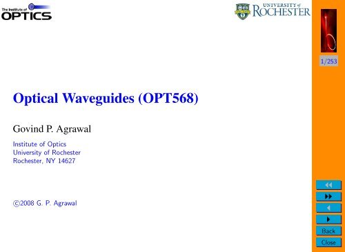
Optical Waveguides (<strong>OPT568</strong>)<br />
Govind P. Agrawal<br />
<strong>Institute</strong> <strong>of</strong> <strong>Optics</strong><br />
<strong>University</strong> <strong>of</strong> <strong>Rochester</strong><br />
<strong>Rochester</strong>, NY 14627<br />
c○2008 G. P. Agrawal<br />
◭◭<br />
◮◮<br />
◭<br />
◮<br />
Back<br />
Close
Introduction<br />
• Optical waveguides confine light inside them.<br />
• Two types <strong>of</strong> waveguides exist:<br />
⋆ Metallic waveguides (coaxial cables,<br />
useful for microwaves).<br />
⋆ Dielectric waveguides (optical fibers).<br />
• This course focuses on dielectric waveguides<br />
and optoelectronic devices made with them.<br />
• Physical Mechanism: Total Internal Reflection.<br />
2/253<br />
◭◭<br />
◮◮<br />
◭<br />
◮<br />
Back<br />
Close
Total Internal Reflection<br />
• Refraction <strong>of</strong> light at a dielectric interface is governed by<br />
Snell’s law: n 1 sinθ i = n 2 sinθ t (around 1620).<br />
• When n 1 > n 2 , light bends away from the normal (θ t > θ i ).<br />
• At a critical angle θ i = θ c , θ t becomes 90 ◦ (parallel to interface).<br />
• Total internal reflection occurs for θ i > θ c .<br />
3/253<br />
◭◭<br />
◮◮<br />
◭<br />
◮<br />
Back<br />
Close
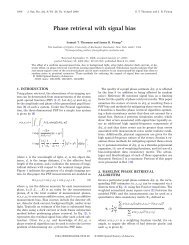
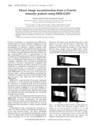
Historical Details<br />
4/253<br />
Daniel Colladon Experimental Setup John Tyndall<br />
• TIR is attributed toJohn Tyndall (1854 experiment in London).<br />
• Book City <strong>of</strong> Light (Jeff Hecht, 1999) traces history <strong>of</strong> TIR.<br />
• First demonstration in Geneva in 1841 by Daniel Colladon<br />
(Comptes Rendus, vol. 15, pp. 800-802, Oct. 24, 1842).<br />
• Light remained confined to a falling stream <strong>of</strong> water.<br />
◭◭<br />
◮◮<br />
◭<br />
◮<br />
Back<br />
Close
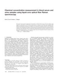
Historical Details<br />
• Tyndall repeated the experiment in a 1854 lecture at the suggestion<br />
<strong>of</strong> Faraday (but Faraday could not recall the original name).<br />
5/253<br />
• Tyndall’s name got attached to TIR because he described the experiment<br />
in his popular book Light and Electricity (around 1860).<br />
• Colladon published an article <strong>The</strong> Colladon Fountain in 1884 to<br />
claim credit but it didn’t work (La Nature, Scientific American).<br />
A fish tank and a laser pointer can be<br />
used to demonstrate the phenomenon<br />
<strong>of</strong> total internal reflection.<br />
◭◭<br />
◮◮<br />
◭<br />
◮<br />
Back<br />
Close
Dielectric Waveguides<br />
6/253<br />
• A thin layer <strong>of</strong> high-index material is sandwiched between two layers.<br />
• Light ray hits the interface at an angle φ = π/2 − θ r<br />
such that n 0 sinθ i = n 1 sinθ r .<br />
• Total internal reflection occurs if φ > φ c = sin −1 (n 2 /n 1 ).<br />
• Numerical aperture is related to maximum angle <strong>of</strong> incidence as<br />
√<br />
NA = n 0 sinθi max = n 1 sin(π/2 − φ c ) = n 2 1 − n2 2 .<br />
◭◭<br />
◮◮<br />
◭<br />
◮<br />
Back<br />
Close
Geometrical-<strong>Optics</strong> Description<br />
• Ray picture valid only within geometrical-optics approximation.<br />
• Useful for a physical understanding <strong>of</strong> waveguiding mechanism.<br />
7/253<br />
• It can be used to show that light remains confined to a waveguide for<br />
only a few specific incident angles angles if one takes into account<br />
the Goos–Hänchen shift (extra phase shift at the interface).<br />
• <strong>The</strong> angles corresponds to waveguide modes in wave optics.<br />
• For thin waveguides, only a single mode exists.<br />
• One must resort to wave-optics description for thin waveguides<br />
(thickness d ∼ λ).<br />
◭◭<br />
◮◮<br />
◭<br />
◮<br />
Back<br />
Close
Maxwell’s Equations<br />
Constitutive Relations<br />
Linear Susceptibility<br />
∇ × E = − ∂B<br />
∂t<br />
∇ × H = ∂D<br />
∂t<br />
∇ · D = 0<br />
∇ · B = 0<br />
D = ε 0 E + P<br />
B = µ 0 H + M<br />
∫ ∞<br />
P(r,t) = ε 0 χ(r,t −t ′ )E(r,t ′ )dt ′<br />
−∞<br />
8/253<br />
◭◭<br />
◮◮<br />
◭<br />
◮<br />
Back<br />
Close
Nonmagnetic Dielectric Materials<br />
• M = 0, and thus B = µ 0 H.<br />
• Linear susceptibility in the Fourier domain: ˜P(ω) = ε 0 χ(ω)Ẽ(ω).<br />
9/253<br />
• Constitutive Relation: ˜D = ε 0 [1 + χ(ω)]Ẽ ≡ ε 0 ε(ω)Ẽ.<br />
• Dielectric constant: ε(ω) = 1 + χ(ω).<br />
• If we use the relation ε = (n + iαc/2ω) 2 ,<br />
n = (1 + Re χ) 1/2 , α = (ω/nc)Im χ.<br />
• Frequency-Domain Maxwell Equations:<br />
∇ × Ẽ = iωµ 0 ˜H, ∇ · (εẼ) = 0<br />
∇ × ˜H = −iωε 0 εẼ, ∇ · ˜H = 0<br />
◭◭<br />
◮◮<br />
◭<br />
◮<br />
Back<br />
Close
Helmholtz Equation<br />
• If losses are small, ε ≈ n 2 .<br />
• Eliminate H from the two curl equations:<br />
10/253<br />
∇ × ∇ × Ẽ = µ 0 ε 0 ω 2 n 2 (ω)Ẽ = ω2<br />
c 2 n2 (ω)Ẽ = k 2 0n 2 (ω)Ẽ.<br />
• Now use the identity<br />
∇ × ∇ × Ẽ ≡ ∇(∇ · Ẽ) − ∇ 2 Ẽ = −∇ 2 Ẽ<br />
• ∇ · Ẽ = 0 only if n is independent <strong>of</strong> r (homogeneous medium).<br />
• We then obtain the Helmholtz equation:<br />
∇ 2 Ẽ + n 2 (ω)k 2 0Ẽ = 0.<br />
◭◭<br />
◮◮<br />
◭<br />
◮<br />
Back<br />
Close
Planar Waveguides<br />
x<br />
11/253<br />
n c<br />
Cover<br />
n 1<br />
y<br />
Core<br />
z<br />
n s<br />
Substrate<br />
• Core film sandwiched between two layers <strong>of</strong> lower refractive index.<br />
• Bottom layer is <strong>of</strong>ten a substrate with n = n s .<br />
• Top layer is called the cover layer (n c ≠ n s ).<br />
• Air can also acts as a cover (n c = 1).<br />
• n c = n s in symmetric waveguides.<br />
◭◭<br />
◮◮<br />
◭<br />
◮<br />
Back<br />
Close
Modes <strong>of</strong> Planar Waveguides<br />
• An optical mode is solution <strong>of</strong> Maxwell’s equations satisfying all<br />
boundary conditions.<br />
12/253<br />
• Its spatial distribution does not change with propagation.<br />
• Modes are obtained by solving the curl equations<br />
∇ × E = iωµ 0 H,<br />
∇ × H = −iωε 0 n 2 E<br />
• <strong>The</strong>se six equations solved in each layer <strong>of</strong> the waveguide.<br />
• Boundary condition: Tangential component <strong>of</strong> E and H be<br />
continuous across both interfaces.<br />
• Waveguide modes are obtained by imposing<br />
the boundary conditions.<br />
◭◭<br />
◮◮<br />
◭<br />
◮<br />
Back<br />
Close
Modes <strong>of</strong> Planar Waveguides<br />
∂E z<br />
∂y − ∂E y<br />
∂z<br />
= iωµ 0 H x ,<br />
∂E x<br />
∂z − ∂E z<br />
∂x = iωµ 0H y ,<br />
∂E y<br />
∂x − ∂E x<br />
∂y<br />
= iωµ 0 H z ,<br />
∂H z<br />
∂y − ∂H y<br />
∂z = iωε 0n 2 E x<br />
∂H x<br />
∂z − ∂H z<br />
∂x = iωε 0n 2 E y<br />
∂H y<br />
∂x − ∂H x<br />
∂y = iωε 0n 2 E z<br />
• Assume waveguide is infinitely wide along the y axis.<br />
• E and H are then y-independent.<br />
• For any mode, all filed components vary with z as exp(iβz). Thus,<br />
∂E<br />
∂y = 0,<br />
∂H<br />
∂y = 0,<br />
∂E<br />
∂z = iβE,<br />
∂H<br />
∂z = iβH.<br />
13/253<br />
◭◭<br />
◮◮<br />
◭<br />
◮<br />
Back<br />
Close
TE and TM Modes<br />
• <strong>The</strong>se equations have two distinct sets <strong>of</strong> linearly polarized solutions.<br />
• For Transverse-Electric (TE) modes, E z = 0 and E x = 0.<br />
14/253<br />
• TE modes are obtained by solving<br />
d 2 E y<br />
dx 2 + (n2 k 2 0 − β 2 )E y = 0,<br />
• Magnetic field components are related to E y as<br />
k 0 = ω √ ε 0 µ 0 = ω/c.<br />
H x = − β<br />
ωµ 0<br />
E y , H y = 0, H z = − i<br />
ωµ 0<br />
dE y<br />
dx .<br />
• For transverse magnetic (TM) modes, H z = 0 and H x = 0.<br />
• Electric filed components are now related to H y as<br />
E x =<br />
β<br />
ωε 0 n 2H y, E y = 0, E z = i<br />
ωε 0 n 2 dH y<br />
dx .<br />
◭◭<br />
◮◮<br />
◭<br />
◮<br />
Back<br />
Close
Solution for TE Modes<br />
d 2 E y<br />
dx + 2 (n2 k0 2 − β 2 )E y = 0.<br />
• We solve this equation in each layer separately using<br />
n = n c , n 1 , and n s .<br />
⎧<br />
⎨<br />
E y (x) =<br />
⎩<br />
B c exp[−q 1 (x − d)]; x > d,<br />
Acos(px − φ) ; |x| ≤ d<br />
B s exp[q 2 (x + d)] ; x < −d,<br />
• Constants p, q 1 , and q 2 are defined as<br />
p 2 = n 2 1k 2 0 − β 2 , q 2 1 = β 2 − n 2 ck 2 0, q 2 2 = β 2 − n 2 sk 2 0.<br />
• Constants B c , B s , A, and φ are determined from the boundary<br />
conditions at the two interfaces.<br />
15/253<br />
◭◭<br />
◮◮<br />
◭<br />
◮<br />
Back<br />
Close
Boundary Conditions<br />
• Tangential components <strong>of</strong> E and H continuous across any interface<br />
with index discontinuity.<br />
16/253<br />
• Mathematically, E y and H z should be continuous at x = ±d.<br />
• E y is continuous at x = ±d if<br />
B c = Acos(pd − φ);<br />
B s = Acos(pd + φ).<br />
• Since H z ∝ dE y /dx, dE y /dx should also be continuous at x = ±d:<br />
pAsin(pd − φ) = q 1 B c , pAsin(pd + φ) = q 2 B s .<br />
• Eliminating A,B c ,B s from these equations, φ must satisfy<br />
tan(pd − φ) = q 1 /p, tan(pd + φ) = q 2 /p<br />
◭◭<br />
◮◮<br />
◭<br />
◮<br />
Back<br />
Close
TE Modes<br />
• Boundary conditions are satisfied when<br />
pd − φ = tan −1 (q 1 /p) + m 1 π, pd + φ = tan −1 (q 2 /p) + m 2 π<br />
17/253<br />
• Adding and subtracting these equations, we obtain<br />
2φ = mπ − tan −1 (q 1 /p) + tan −1 (q 2 /p)<br />
2pd = mπ + tan −1 (q 1 /p) + tan −1 (q 2 /p)<br />
• <strong>The</strong> last equation is called the eigenvalue equation.<br />
• Multiple solutions for m = 0,1,2,... are denoted by TE m .<br />
• Effective index <strong>of</strong> each TE mode is ¯n = β/k 0 .<br />
◭◭<br />
◮◮<br />
◭<br />
◮<br />
Back<br />
Close
TM Modes<br />
• Same procedure is used to obtain TM modes.<br />
• Solution for H y has the same form in three layers.<br />
18/253<br />
• Continuity <strong>of</strong> E z requires that n −2 (dH y /dx) be continuous<br />
at x = ±d.<br />
• Since n is different on the two sides <strong>of</strong> each interface,<br />
eigenvalue equation is modified to become<br />
( ) ( )<br />
n<br />
2pd = mπ + tan −1 2<br />
1 q 1 n<br />
+ tan −1 2<br />
1 q 2<br />
.<br />
n 2 c p<br />
n 2 s p<br />
• Multiple solutions for different values <strong>of</strong> m.<br />
• <strong>The</strong>se are labelled as TM m modes.<br />
◭◭<br />
◮◮<br />
◭<br />
◮<br />
Back<br />
Close
TE Modes <strong>of</strong> Symmetric Waveguides<br />
• For symmetric waveguides n c = n s .<br />
• Using q 1 = q 2 ≡ q, TE modes satisfy<br />
19/253<br />
• Define a dimensionless parameter<br />
q = ptan(pd − mπ/2).<br />
V = d √ p 2 + q 2 = k 0 d<br />
√<br />
n 2 1 − n2 s,<br />
• If we use u = pd, the eigenvalue equation can be written as<br />
√<br />
V<br />
2<br />
− u 2 = utan(u − mπ/2).<br />
• For given values <strong>of</strong> V and m, this equation is solved to find p = u/d.<br />
◭◭<br />
◮◮<br />
◭<br />
◮<br />
Back<br />
Close
TE Modes <strong>of</strong> Symmetric Waveguides<br />
• Effective index ¯n = β/k 0 = (n 2 1 − p2 /k 2 0 )1/2 .<br />
• Using 2φ = mπ − tan −1 (q 1 /p) + tan −1 (q 2 /p)<br />
with q 1 = q 2 , phase φ = mπ/2.<br />
• Spatial distribution <strong>of</strong> modes is found to be<br />
{<br />
B± exp[−q(|x| − d)]; |x| > d,<br />
E y (x) =<br />
Acos(px − mπ/2) ; |x| ≤ d,<br />
where B ± = Acos(pd ∓ mπ/2) and the lower sign is chosen for<br />
x < 0.<br />
• Modes with even values <strong>of</strong> m are symmetric around<br />
x = 0 (even modes).<br />
• Modes with odd values <strong>of</strong> m are antisymmetric around<br />
x = 0 (odd modes).<br />
20/253<br />
◭◭<br />
◮◮<br />
◭<br />
◮<br />
Back<br />
Close
TM Modes <strong>of</strong> Symmetric Waveguides<br />
• We can follow the same procedure for TM modes.<br />
• Eigenvalue equation for TM modes:<br />
21/253<br />
(n 1 /n s ) 2 q = ptan(pd − mπ/2).<br />
• TM modes can also be divided into even and odd modes.<br />
◭◭<br />
◮◮<br />
◭<br />
◮<br />
Back<br />
Close
Symmetric Waveguides<br />
• TE 0 and TM 0 modes have no nodes within the core.<br />
• <strong>The</strong>y are called the fundamental modes <strong>of</strong> a planar waveguide.<br />
• Number <strong>of</strong> modes supported by a waveguide depends on the V<br />
parameter.<br />
• A mode ceases to exist when q = 0 (no longer confined to the core).<br />
• This occurs for both TE and TM modes when V = V m = mπ/2.<br />
• Number <strong>of</strong> modes = Largest value <strong>of</strong> m for which V m > V .<br />
• A waveguide with V = 10 supports 7 TE and 7 TM modes<br />
(V 6 = 9.42 but V 7 exceeds 10).<br />
• A waveguide supports a single TE and a single TM mode when<br />
V < π/2 (single-mode condition).<br />
22/253<br />
◭◭<br />
◮◮<br />
◭<br />
◮<br />
Back<br />
Close
Modes <strong>of</strong> Asymmetric Waveguides<br />
• We can follow the same procedure for n c ≠ n s .<br />
• Eigenvalue equation for TE modes:<br />
2pd = mπ + tan −1 (q 1 /p) + tan −1 (q 2 /p)<br />
• Eigenvalue equation for TM modes:<br />
2pd = mπ + tan −1 ( n<br />
2<br />
1 q 1<br />
n 2 c p<br />
• Constants p, q 1 , and q 2 are defined as<br />
) ( ) n<br />
+ tan −1 2<br />
1 q 2<br />
n 2 s p<br />
p 2 = n 2 1k 2 0 − β 2 , q 2 1 = β 2 − n 2 ck 2 0, q 2 2 = β 2 − n 2 sk 2 0.<br />
• Each solution for β corresponds to a mode with effective index<br />
¯n = β/k 0 .<br />
• If n 1 > n s > n c , guided modes exist as long as n 1 > ¯n > n s .<br />
23/253<br />
◭◭<br />
◮◮<br />
◭<br />
◮<br />
Back<br />
Close
Modes <strong>of</strong> Asymmetric Waveguides<br />
• Useful to introduce two normalized parameters as<br />
24/253<br />
b = ¯n2 − n 2 s<br />
n 2 1 − n2 s<br />
, δ = n2 s − n 2 c<br />
n 2 1 − .<br />
n2 s<br />
• b is a normalized propagation constant (0 < b < 1).<br />
• Parameter δ provides a measure <strong>of</strong> waveguide asymmetry.<br />
• Eigenvalue equation for TE modes in terms V,b,δ:<br />
2V √ √<br />
√<br />
b<br />
b + δ<br />
1 − b = mπ + tan −1 1 − b + tan−1 1 − b .<br />
• Its solutions provide universal dispersion curves.<br />
◭◭<br />
◮◮<br />
◭<br />
◮<br />
Back<br />
Close
Modes <strong>of</strong> Asymmetric Waveguides<br />
Normalized propagation constant, b<br />
1<br />
0.9<br />
0.8<br />
0.7<br />
0.6<br />
0.5<br />
0.4<br />
0.3<br />
0.2<br />
0.1<br />
m = 0<br />
0<br />
0 1 2 3 4 5 6 7 8 9 10<br />
Normalized frequency, V<br />
Solid lines (δ = 5); dashed lines (δ = 0).<br />
1<br />
2<br />
3<br />
4<br />
5<br />
25/253<br />
◭◭<br />
◮◮<br />
◭<br />
◮<br />
Back<br />
Close
Mode-Cut<strong>of</strong>f Condition<br />
• Cut<strong>of</strong>f condition corresponds to the value <strong>of</strong> V for which mode<br />
ceases to decay exponentially in one <strong>of</strong> the cladding layers.<br />
• It is obtained by setting b = 0 in eigenvalue equation:<br />
V m (TE) = mπ<br />
2 + 1 2 tan−1 √ δ.<br />
• Eigenvalue equation for the TM modes:<br />
2V √ ( √ ) (<br />
1 − b = mπ + tan −1 n 2 1 b<br />
+ tan −1<br />
1 − b<br />
• <strong>The</strong> cut<strong>of</strong>f condition found by setting b = 0:<br />
V m (TM) = mπ<br />
2 + 1 ( n<br />
2√ )<br />
1<br />
2 tan−1 δ .<br />
n 2 c<br />
n 2 s<br />
n 2 1<br />
n 2 c<br />
√ )<br />
b + δ<br />
.<br />
1 − b<br />
26/253<br />
◭◭<br />
◮◮<br />
◭<br />
◮<br />
Back<br />
Close
Mode-Cut<strong>of</strong>f Condition<br />
• For a symmetric waveguide (δ = 0), these two conditions reduce to<br />
a single condition, V m = mπ/2.<br />
27/253<br />
• TE and TM modes for a given value <strong>of</strong> m have the same cut<strong>of</strong>f.<br />
• A single-mode waveguide is realized if V parameter <strong>of</strong> the waveguide<br />
satisfies<br />
√<br />
V ≡ k 0 d n 2 1 − n2 s < π 2<br />
• Fundamental mode always exists for a symmetric waveguide.<br />
• An asymmetric waveguide with 2V < tan −1 √ δ does not support<br />
any bounded mode.<br />
◭◭<br />
◮◮<br />
◭<br />
◮<br />
Back<br />
Close
Spatial Distribution <strong>of</strong> Modes<br />
⎧<br />
⎨ B c exp[−q 1 (x − d)]; x > d,<br />
E y (x) = Acos(px − φ) ; |x| ≤ d<br />
⎩<br />
B s exp[q 2 (x + d)] ; x < −d,<br />
• Boundary conditions: B c = Acos(pd − φ), B s = Acos(pd + φ)<br />
• A is related to total power P = 1 ∫ ∞<br />
2 −∞ ẑ · (E × H)dx:<br />
P =<br />
β<br />
2ωµ 0<br />
∫ ∞<br />
−∞<br />
|E y (x)| 2 dx = βA2<br />
4ωµ 0<br />
(<br />
2d + 1 q 1<br />
+ 1 q 2<br />
).<br />
• Fraction <strong>of</strong> power propagating inside the waveguide layer:<br />
∫ d<br />
−d<br />
Γ =<br />
|E y(x)| 2 dx<br />
∫ ∞<br />
−∞ |E y(x)| 2 dx = 2d + sin2 (pd − φ)/q 1 + sin 2 (pd + φ)/q 2<br />
.<br />
2d + 1/q 1 + 1/q 2<br />
• For fundamental mode Γ ≪ 1 when V ≪ π/2.<br />
28/253<br />
◭◭<br />
◮◮<br />
◭<br />
◮<br />
Back<br />
Close
Rectangular Waveguides<br />
• Rectangular waveguide confines light in both x and y dimensions.<br />
• <strong>The</strong> high-index region in the middle core layer has a finite width 2w<br />
and is surrounded on all sides by lower-index materials.<br />
• Refractive index can be different on all sides <strong>of</strong> a rectangular waveguide.<br />
29/253<br />
◭◭<br />
◮◮<br />
◭<br />
◮<br />
Back<br />
Close
Modes <strong>of</strong> Rectangular Waveguides<br />
• To simplify the analysis, all shaded cladding regions are assumed to<br />
have the same refractive index n c .<br />
30/253<br />
• A numerical approach still necessary for an exact solution.<br />
• Approximate analytic solution possible with two simplifications;<br />
Marcatili, Bell Syst. Tech. J. 48, 2071 (1969).<br />
⋆ Ignore boundary conditions associated with hatched regions.<br />
⋆ Assume core-cladding index differences are small on all sides.<br />
• Problem is then reduced to solving two planar-waveguide problems<br />
in the x and y directions.<br />
◭◭<br />
◮◮<br />
◭<br />
◮<br />
Back<br />
Close
Modes <strong>of</strong> Rectangular Waveguides<br />
• One can find TE- and TM-like modes for which either E z or H z is<br />
nearly negligible compared to other components.<br />
31/253<br />
• Modes denoted as E x mn and E y mn obtained by solving two coupled<br />
eigenvalue equations.<br />
( ) ( )<br />
n<br />
2p x d = mπ + tan −1 2<br />
1 q 2 n<br />
n 2 2 p + tan −1 2<br />
1 q 4<br />
x n 2 4 p ,<br />
x<br />
( ) ( )<br />
2p y w = nπ + tan −1 q3<br />
+ tan −1 q5<br />
,<br />
p y p y<br />
p 2 x = n 2 1k 2 0 − β 2 − p 2 y, p 2 y = n 2 1k 2 0 − β 2 − p 2 x,<br />
q 2 2 = β 2 + p 2 y − n 2 2k 2 0, q 2 4 = β 2 + p 2 y − n 2 4k 2 0,<br />
q 2 3 = β 2 + p 2 x − n 2 3k 2 0, q 2 5 = β 2 + p 2 x − n 2 5k 2 0,<br />
◭◭<br />
◮◮<br />
◭<br />
◮<br />
Back<br />
Close
Effective-Index Method<br />
• Effective-index method appropriate when thickness <strong>of</strong> a rectangular<br />
waveguide is much smaller than its width (d ≪ w).<br />
32/253<br />
• Planar waveguide problem in the x direction is solved first to obtain<br />
the effective mode index n e (y).<br />
• n e is a function <strong>of</strong> y because <strong>of</strong> a finite waveguide width.<br />
• In the y direction, we use a waveguide <strong>of</strong> width 2w such that n y = n e<br />
if |y| < w but equals n 3 or n 5 outside <strong>of</strong> this region.<br />
• Single-mode condition is found to be<br />
V x = k 0 d<br />
√<br />
n 2 1 − n2 4 < π/2,<br />
√<br />
V y = k 0 w n 2 e − n 2 5 < π/2<br />
◭◭<br />
◮◮<br />
◭<br />
◮<br />
Back<br />
Close
Design <strong>of</strong> Rectangular Waveguides<br />
33/253<br />
• In (g) core layer is covered with two metal stripes.<br />
• Losses can be reduced by using a thin buffer layer (h).<br />
◭◭<br />
◮◮<br />
◭<br />
◮<br />
Back<br />
Close
Materials for Waveguides<br />
• Semiconductor Waveguides: GaAs, InP, etc.<br />
• Electro-Optic Waveguides: mostly LiNbO 3 .<br />
• Glass Waveguides: silica (SiO 2 ), SiON.<br />
⋆ Silica-on-silicon technology<br />
⋆ Laser-written waveguides<br />
• Silicon-on-Insulator Technology<br />
• Polymers Waveguides: Several organic<br />
polymers<br />
34/253<br />
◭◭<br />
◮◮<br />
◭<br />
◮<br />
Back<br />
Close
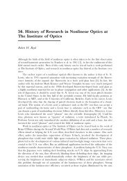
Semiconductor Waveguides<br />
Useful for semiconductor lasers, modulators, and photodetectors.<br />
• Semiconductors allow fabrication<br />
<strong>of</strong> electrically active devices.<br />
35/253<br />
• Semiconductors belonging to III–<br />
V Group <strong>of</strong>ten used.<br />
• Two semiconductors with different<br />
refractive indices needed.<br />
• <strong>The</strong>y must have different<br />
bandgaps but same lattice<br />
constant.<br />
• Nature does not provide such<br />
semiconductors.<br />
◭◭<br />
◮◮<br />
◭<br />
◮<br />
Back<br />
Close
Ternary and Quaternary Compounds<br />
• A fraction <strong>of</strong> the lattice sites in a binary semiconductor (GaAs, InP,<br />
etc.) is replaced by other elements.<br />
36/253<br />
• Ternary compound Al x Ga 1−x As is made by replacing a fraction x <strong>of</strong><br />
Ga atoms by Al atoms.<br />
• Bandgap varies with x as<br />
E g (x) = 1.424 + 1.247x (0 < x < 0.45).<br />
• Quaternary compound In 1−x Ga x As y P 1−y useful in the wavelength<br />
range 1.1 to 1.6 µm.<br />
• For matching lattice constant to InP substrate, x/y = 0.45.<br />
• Bandgap varies with y as E g (y) = 1.35 − 0.72y + 0.12y 2 .<br />
◭◭<br />
◮◮<br />
◭<br />
◮<br />
Back<br />
Close
Fabrication Techniques<br />
Epitaxial growth <strong>of</strong> multiple layers on a base substrate (GaAs or InP).<br />
Three primary techniques:<br />
37/253<br />
• Liquid-phase epitaxy (LPE)<br />
• Vapor-phase epitaxy (VPE)<br />
• Molecular-beam epitaxy (MBE)<br />
VPE is also called chemical-vapor<br />
deposition (CVD).<br />
Metal-organic chemical-vapor deposition (MOCVD) is <strong>of</strong>ten used in<br />
practice.<br />
◭◭<br />
◮◮<br />
◭<br />
◮<br />
Back<br />
Close
Quantum-Well Technology<br />
• Thickness <strong>of</strong> the core layer plays a central role.<br />
• If it is small enough, electrons and holes act as if they are confined<br />
to a quantum well.<br />
38/253<br />
• Confinement leads to quantization <strong>of</strong> energy bands into subbands.<br />
• Joint density <strong>of</strong> states acquires a staircase-like structure.<br />
• Useful for making modern quantum-well, quantum wire, and<br />
quantum-dot lasers.<br />
• in MQW lasers, multiple core layers (thickness 5–10 nm) are<br />
separated by transparent barrier layers.<br />
• Use <strong>of</strong> intentional but controlled strain improves performance<br />
in strained quantum wells.<br />
◭◭<br />
◮◮<br />
◭<br />
◮<br />
Back<br />
Close
Doped Semiconductor Waveguides<br />
• To build a laser, one needs to inject current into the core layer.<br />
• This is accomplished through a p–n junction formed by<br />
making cladding layers p- and n-types.<br />
39/253<br />
• n-type material requires a dopant with an extra electron.<br />
• p-type material requires a dopant with one less electron.<br />
• Doping creates free electrons or holes within a semiconductor.<br />
• Fermi level lies in the middle <strong>of</strong> bandgap for undoped<br />
(intrinsic) semiconductors.<br />
• In a heavily doped semiconductor, Fermi level lies inside<br />
the conduction or valence band.<br />
◭◭<br />
◮◮<br />
◭<br />
◮<br />
Back<br />
Close
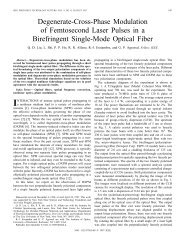
p–n junctions<br />
• Fermi level continuous across the<br />
p–n junction in thermal equilibrium.<br />
40/253<br />
• A built-in electric field separates<br />
electrons and holes.<br />
• Forward biasing reduces the builtin<br />
electric field.<br />
• An electric current begins to flow:<br />
I = I s [exp(qV /k B T ) − 1].<br />
• Recombination <strong>of</strong> electrons and<br />
holes generates light.<br />
(a)<br />
(b)<br />
◭◭<br />
◮◮<br />
◭<br />
◮<br />
Back<br />
Close
Electro-Optic Waveguides<br />
• Use Pockels effect to change refractive index <strong>of</strong> the core layer with<br />
an external voltage.<br />
41/253<br />
• Common electro-optic materials: LiNbO 3 , LiTaO 3 , BaTiO 3 .<br />
• LiNbO 3 used commonly for making optical modulators.<br />
• For any anisotropic material D i = ε 0 ∑ 3 j=1 ε i j E j .<br />
• Matrix ε i j can be diagonalized by rotating the coordinate system<br />
along the principal axes.<br />
• Impermeability tensor η i j = 1/ε i j describes changes induced by an<br />
external field as η i j (E a ) = η i j (0) + ∑ k r i jk E a k .<br />
• Tensor r i jk is responsible for the electro-optic effect.<br />
◭◭<br />
◮◮<br />
◭<br />
◮<br />
Back<br />
Close
Lithium Niobate Waveguides<br />
• LiNbO 3 waveguides do not require an epitaxial growth.<br />
• A popular technique employs diffusion <strong>of</strong> metals into a LiNbO 3 substrate,<br />
resulting in a low-loss waveguide.<br />
42/253<br />
• <strong>The</strong> most commonly used element: Titanium (Ti).<br />
• Diffusion <strong>of</strong> Ti atoms within LiNbO 3 crystal increases refractive<br />
index and forms the core region.<br />
• Out-diffusion <strong>of</strong> Li atoms from substrate should be avoided.<br />
• Surface flatness critical to ensure a uniform waveguide.<br />
◭◭<br />
◮◮<br />
◭<br />
◮<br />
Back<br />
Close
LiNbO 3 Waveguides<br />
• A proton-exchange technique is also used for LiNbO 3 waveguides.<br />
• A low-temperature process (∼ 200 ◦ C) in which Li ions are replaced<br />
with protons when the substrate is placed in an acid bath.<br />
43/253<br />
• Proton exchange increases the extraordinary part <strong>of</strong> refractive index<br />
but leaves the ordinary part unchanged.<br />
• Such a waveguide supports only TM modes and is useful for some<br />
applications because <strong>of</strong> its polarization selectivity.<br />
• High-temperature annealing used to stabilizes the index difference.<br />
• Accelerated aging tests predict a lifetime <strong>of</strong> over 25 years at a temperature<br />
as high as 95 ◦ C.<br />
◭◭<br />
◮◮<br />
◭<br />
◮<br />
Back<br />
Close
LiNbO 3 Waveguides<br />
44/253<br />
• Electrodes fabricated directly on the surface <strong>of</strong> wafer (or on<br />
an optically transparent buffer layer.<br />
• An adhesion layer (typically Ti) first deposited to ensure that<br />
metal sticks to LiNbO 3 .<br />
• Photolithography used to define the electrode pattern.<br />
◭◭<br />
◮◮<br />
◭<br />
◮<br />
Back<br />
Close
Silica Glass Waveguides<br />
• Silica layers deposited on top <strong>of</strong> a Si substrate.<br />
• Employs the technology developed for integrated circuits.<br />
45/253<br />
• Fabricated using flame hydrolysis with reactive ion etching.<br />
• Two silica layers are first deposited using flame hydrolysis.<br />
• Top layer converted to core by doping it with germania.<br />
• Both layers solidified by heating at 1300 ◦ C (consolidation process).<br />
• Photolithography used to etch patterns on the core layer.<br />
• Entire structure covered with a cladding formed using flame hydrolysis.<br />
A thermo-optic phase shifter <strong>of</strong>ten formed on top.<br />
◭◭<br />
◮◮<br />
◭<br />
◮<br />
Back<br />
Close
Silica-on-Silicon Technique<br />
46/253<br />
Steps used to form silica waveguides on top <strong>of</strong> a Si Substrate<br />
◭◭<br />
◮◮<br />
◭<br />
◮<br />
Back<br />
Close
Silica Waveguide properties<br />
• Silica-on-silicon technology produces uniform waveguides.<br />
• Losses depend on the core-cladding index difference<br />
∆ = (n 1 − n 2 )/n 1 .<br />
• Losses are low for small values <strong>of</strong> ∆ (about 0.017 dB/cm<br />
for ∆ = 0.45%).<br />
• Higher values <strong>of</strong> ∆ <strong>of</strong>ten used for reducing device length.<br />
• Propagation losses ∼0.1 dB/cm for ∆ = 2%.<br />
• Planar lightwave circuits: Multiple waveguides and optical<br />
components integrated over the same silicon substrate.<br />
• Useful for making compact WDM devices (∼ 5 × 5 cm 2 ).<br />
• Large insertion losses when a PLC is connected to optical fibers.<br />
47/253<br />
◭◭<br />
◮◮<br />
◭<br />
◮<br />
Back<br />
Close
Packaged PLCs<br />
48/253<br />
• Package design for minimizing insertion losses.<br />
• Fibers inserted into V-shaped grooves formed on a glass substrate.<br />
• Glass substrate connected to the PLC chip using an adhesive.<br />
• A glass plate placed on top <strong>of</strong> V grooves is bonded to the PLC chip<br />
◭◭<br />
◮◮<br />
◭<br />
◮<br />
Back<br />
Close
with the same adhesive.<br />
49/253<br />
◭◭<br />
◮◮<br />
◭<br />
◮<br />
Back<br />
Close
Silicon Oxynitride Waveguides<br />
• Employ Si substrate but use SiON for the core layer.<br />
• SiON alloy is made by combining SiO 2 with Si 3 N 4 , two dielectrics<br />
with refractive indices <strong>of</strong> 1.45 and 2.01.<br />
50/253<br />
• Refractive index <strong>of</strong> SiON layer can vary from 1.45–2.01.<br />
• SiON film deposited using plasma-enhanced chemical vapor<br />
deposition (SiH 4 combined with N 2 O and NH 3 ).<br />
• Low-pressure chemical vapor deposition also used<br />
(SiH 2 Cl 2 combined with O 2 and NH 3 ).<br />
• Photolithography pattern formed on a 200-nm-thick chromium layer.<br />
• Propagation losses typically
Laser-Written Waveguides<br />
• CW or pulsed light from a laser used for “writing” waveguides in<br />
silica and other glasses.<br />
51/253<br />
• Photosensitivity <strong>of</strong> germanium-doped silica exploited to enhance<br />
refractive index in the region exposed to a UV laser.<br />
• Absorption <strong>of</strong> 244-nm light from a KrF laser changes refractive index<br />
by ∼10 −4 only in the region exposed to UV light.<br />
• Index changes >10 −3 can be realized with a 193-nm ArF laser.<br />
• A planar waveguide formed first through CVD, but core layer is<br />
doped with germania.<br />
• An UV beam focused to ∼1 µm scanned slowly to enhance n selectively.<br />
UV-written sample then annealed at 80 ◦ C.<br />
◭◭<br />
◮◮<br />
◭<br />
◮<br />
Back<br />
Close
Laser-Written Waveguides<br />
52/253<br />
• Femtosecond pulses from a Ti:sapphire laser can be used to write<br />
waveguides in bulk glasses.<br />
• Intense pulses modify the structure <strong>of</strong> silica through<br />
multiphoton absorption.<br />
• Refractive-index changes ∼10 −2 are possible.<br />
◭◭<br />
◮◮<br />
◭<br />
◮<br />
Back<br />
Close
Silicon-on-Insulator Technology<br />
53/253<br />
• Core waveguide layer is made <strong>of</strong> Si (n 1 = 3.45).<br />
• A silica layer under the core layer is used for lower cladding.<br />
• Air on top acts as the top cladding layer.<br />
• Tightly confined waveguide mode because <strong>of</strong> large index difference.<br />
• Silica layer formed by implanting oxygen, followed with annealing.<br />
◭◭<br />
◮◮<br />
◭<br />
◮<br />
Back<br />
Close
Polymer Waveguides<br />
54/253<br />
• Polymers such as halogenated acrylate, fluorinated polyimide, and<br />
deuterated polymethylmethacrylate (PMMA) have been used.<br />
• Polymer films can be fabricated on top <strong>of</strong> Si, glass, quartz,<br />
or plastic through spin coating.<br />
• Photoresist layer on top used for reactive ion etching <strong>of</strong> the core<br />
layer through a photomask.<br />
◭◭<br />
◮◮<br />
◭<br />
◮<br />
Back<br />
Close
Optical Fibers<br />
55/253<br />
• Contain a central core surrounded by a lower-index cladding<br />
• Two-dimensional waveguides with cylindrical symmetry<br />
• Graded-index fibers: Refractive index varies inside the core<br />
◭◭<br />
◮◮<br />
◭<br />
◮<br />
Back<br />
Close
Total internal reflection<br />
• Refraction at the air–glass interface:<br />
n 0 sinθ i = n 1 sinθ r<br />
• Total internal reflection at the core-cladding interface<br />
if φ > φ c = sin −1 (n 2 /n 1 ).<br />
56/253<br />
Numerical Aperture: Maximum angle <strong>of</strong> incidence<br />
n 0 sinθ max<br />
i = n 1 sin(π/2 − φ c ) = n 1 cosφ c =<br />
√<br />
n 2 1 − n2 2<br />
◭◭<br />
◮◮<br />
◭<br />
◮<br />
Back<br />
Close
Modal Dispersion<br />
• Multimode fibers suffer from modal dispersion.<br />
• Shortest path length L min = L (along the fiber axis).<br />
• Longest path length for the ray close to the critical angle<br />
57/253<br />
L max = L/sinφ c = L(n 1 /n 2 ).<br />
• Pulse broadening: ∆T = (L max − L min )(n 1 /c).<br />
• Modal dispersion: ∆T /L = n 2 1 ∆/(n 2c).<br />
• Limitation on the bit rate<br />
∆T < T B = 1/B; B∆T < 1; BL < n 2c<br />
n 2 1 ∆.<br />
• Single-mode fibers essential for high performance.<br />
◭◭<br />
◮◮<br />
◭<br />
◮<br />
Back<br />
Close
Graded-Index Fibers<br />
58/253<br />
• Refractive index n(ρ) =<br />
{<br />
n1 [1 − ∆(ρ/a) α ]; ρ < a,<br />
n 1 (1 − ∆) = n 2 ; ρ ≥ a.<br />
• Ray path obtained by solving d2 ρ<br />
= 1 dn<br />
dz 2 n dρ .<br />
• For α = 2, ρ = ρ 0 cos(pz) + (ρ ′ 0 /p)sin(pz).<br />
• All rays arrive simultaneously at periodic intervals.<br />
• Limitation on the Bit Rate: BL < 8c<br />
n 1 ∆ 2 .<br />
◭◭<br />
◮◮<br />
◭<br />
◮<br />
Back<br />
Close
Fiber Design<br />
59/253<br />
• Core doped with GeO 2 ; cladding with fluorine.<br />
• Index pr<strong>of</strong>ile rectangular for standard fibers.<br />
• Triangular index pr<strong>of</strong>ile for dispersion-shifted fibers.<br />
• Raised or depressed cladding for dispersion control.<br />
◭◭<br />
◮◮<br />
◭<br />
◮<br />
Back<br />
Close
Silica Fibers<br />
Two-Stage Fabrication<br />
• Preform: Length 1 m, diameter 2 cm; correct index pr<strong>of</strong>ile.<br />
• Preform is drawn into fiber using a draw tower.<br />
60/253<br />
Preform Fabrication Techniques<br />
• Modified chemical vapor deposition (MCVD).<br />
• Outside vapor deposition (OVD).<br />
• Vapor Axial deposition (VAD).<br />
◭◭<br />
◮◮<br />
◭<br />
◮<br />
Back<br />
Close
Fiber Draw Tower<br />
61/253<br />
◭◭<br />
◮◮<br />
◭<br />
◮<br />
Back<br />
Close
Plastic Fibers<br />
• Multimode fibers (core diameter as large as 1 mm).<br />
• Large NA results in high coupling efficiency.<br />
62/253<br />
• Use <strong>of</strong> plastics reduces cost but loss exceeds 50 dB/km.<br />
• Useful for data transmission over short distances (
Plastic Fibers<br />
• Preform made with the interfacial gel polymerization method.<br />
• A cladding cylinder is filled with a mixture <strong>of</strong> monomer (same<br />
used for cladding polymer), index-increasing dopant, a chemical for<br />
initiating polymerization, and a chain-transfer agent.<br />
63/253<br />
• Cylinder heated to a 95 ◦ C and rotated on its axis for a period <strong>of</strong><br />
up to 24 hours.<br />
• Core polymerization begins near cylinder wall.<br />
• Dopant concentration increases toward core center.<br />
• This technique automatically creates a gradient in the core index.<br />
◭◭<br />
◮◮<br />
◭<br />
◮<br />
Back<br />
Close
Microstructure Fibers<br />
64/253<br />
• New types <strong>of</strong> fibers with air holes in cladding region.<br />
• Air holes reduce the index <strong>of</strong> the cladding region.<br />
• Narrow core (2 µm or so) results in tighter mode confinement.<br />
• Air-core fibers guide light through the photonic-crystal effect.<br />
• Preform made by stacking silica tubes in a hexagonal pattern.<br />
◭◭<br />
◮◮<br />
◭<br />
◮<br />
Back<br />
Close
Fiber Modes<br />
• Maxwell’s equations in the Fourier domain lead to<br />
∇ 2 Ẽ + n 2 (ω)k 2 0Ẽ = 0.<br />
65/253<br />
• n = n 1 inside the core but changes to n 2 in the cladding.<br />
• Useful to work in cylindrical coordinates ρ,φ,z.<br />
• Common to choose E z and H z as independent components.<br />
• Equation for E z in cylindrical coordinates:<br />
∂ 2 E z<br />
∂ρ + 1 ∂E z<br />
2 ρ ∂ρ + 1 ∂ 2 E z<br />
ρ 2 ∂φ + ∂ 2 E z<br />
2 ∂z + 2 n2 k0E 2 z = 0.<br />
• H z satisfies the same equation.<br />
◭◭<br />
◮◮<br />
◭<br />
◮<br />
Back<br />
Close
Fiber Modes (cont.)<br />
• Use the method <strong>of</strong> separation <strong>of</strong> variables:<br />
• We then obtain three ODEs:<br />
E z (ρ,φ,z) = F(ρ)Φ(φ)Z(z).<br />
d 2 Z/dz 2 + β 2 Z = 0,<br />
d 2 Φ/dφ 2 + m 2 Φ = 0,<br />
d 2 F<br />
dρ + 1 (<br />
)<br />
dF<br />
2 ρ dρ + n 2 k0 2 − β 2 − m2<br />
F = 0.<br />
ρ 2<br />
• β and m are two constants (m must be an integer).<br />
• First two equations can be solved easily to obtain<br />
Z(z) = exp(iβz),<br />
• F(ρ) satisfies the Bessel equation.<br />
Φ(φ) = exp(imφ).<br />
66/253<br />
◭◭<br />
◮◮<br />
◭<br />
◮<br />
Back<br />
Close
Fiber Modes (cont.)<br />
• General solution for E z and H z :<br />
{ AJm (pρ)exp(imφ)exp(iβz) ; ρ ≤ a,<br />
E z =<br />
CK m (qρ)exp(imφ)exp(iβz); ρ > a.<br />
67/253<br />
H z =<br />
{ BJm (pρ)exp(imφ)exp(iβz) ; ρ ≤ a,<br />
DK m (qρ)exp(imφ)exp(iβz); ρ > a.<br />
p 2 = n 2 1 k2 0 − β 2 , q 2 = β 2 − n 2 2 k2 0 .<br />
• Other components can be written in terms <strong>of</strong> E z and H z :<br />
E ρ = i (<br />
β ∂E )<br />
z<br />
p 2 ∂ρ + µ ω ∂H z<br />
0 , E φ = i ( β<br />
ρ ∂φ<br />
p 2 ρ<br />
H ρ = i<br />
p 2 (<br />
β ∂H z<br />
∂ρ − ε 0n 2ω ρ<br />
∂E z<br />
∂φ<br />
∂E z<br />
∂φ − µ 0ω ∂H z<br />
∂ρ<br />
)<br />
,<br />
)<br />
, H φ = i ( β ∂H z<br />
p 2 ρ ∂φ + ε 0n 2 ω ∂E z<br />
∂ρ<br />
)<br />
.<br />
◭◭<br />
◮◮<br />
◭<br />
◮<br />
Back<br />
Close
Eigenvalue Equation<br />
• Boundary conditions: E z , H z , E φ , and H φ<br />
across the core–cladding interface.<br />
should be continuous<br />
68/253<br />
• Continuity <strong>of</strong> E z and H z at ρ = a leads to<br />
AJ m (pa) = CK m (qa), BJ m (pa) = DK m (qa).<br />
• Continuity <strong>of</strong> E φ and H φ provides two more equations.<br />
• Four equations lead to the eigenvalue equation<br />
[ ][ J<br />
′<br />
m (pa)<br />
pJ m (pa) + K′ m(qa) J<br />
′<br />
m (pa)<br />
qK m (qa) pJ m (pa) + n2 2<br />
n 2 1<br />
(<br />
= m2 1<br />
a 2 p + 1 )( ) 1 2 q 2 p + n2 2 1<br />
2 n 2 1<br />
q 2<br />
p 2 = n 2 1 k2 0 − β 2 , q 2 = β 2 − n 2 2 k2 0 .<br />
K ′ m(qa)<br />
qK m (qa)<br />
]<br />
◭◭<br />
◮◮<br />
◭<br />
◮<br />
Back<br />
Close
Eigenvalue Equation<br />
• Eigenvalue equation involves Bessel functions and their derivatives.<br />
It needs to be solved numerically.<br />
69/253<br />
• Noting that p 2 + q 2 = (n 2 1 − n2 2 )k2 0 , we introduce the dimensionless<br />
V parameter as<br />
√<br />
V = k 0 a n 2 1 − n2 2 .<br />
• Multiple solutions for β for a given value <strong>of</strong> V .<br />
• Each solution represents an optical mode.<br />
• Number <strong>of</strong> modes increases rapidly with V parameter.<br />
• Effective mode index ¯n = β/k 0 lies between n 1 and n 2 for all bound<br />
modes.<br />
◭◭<br />
◮◮<br />
◭<br />
◮<br />
Back<br />
Close
Effective Mode Index<br />
70/253<br />
• Useful to introduce a normalized quantity<br />
b = ( ¯n − n 2 )/(n 1 − n 2 ), (0 < b < 1).<br />
• Modes quantified through β(ω) or b(V ).<br />
◭◭<br />
◮◮<br />
◭<br />
◮<br />
Back<br />
Close
Classification <strong>of</strong> Fiber Modes<br />
• In general, both E z and H z are nonzero (hybrid modes).<br />
• Multiple solutions occur for each value <strong>of</strong> m.<br />
71/253<br />
• Modes denoted by HE mn or EH mn (n = 1,2,...) depending on whether<br />
H z or E z dominates.<br />
• TE and TM modes exist for m = 0 (called TE 0n and TM 0n ).<br />
• Setting m = 0 in the eigenvalue equation, we obtain two equations<br />
[ ] [ J<br />
′<br />
m (pa)<br />
pJ m (pa) + K′ m(qa)<br />
J<br />
′<br />
= 0, m (pa)<br />
qK m (qa)<br />
pJ m (pa) + n2 2 K ′ ]<br />
m(qa)<br />
n 2 = 0<br />
1<br />
qK m (qa)<br />
• <strong>The</strong>se equations govern TE 0n and TM 0n modes <strong>of</strong> fiber.<br />
◭◭<br />
◮◮<br />
◭<br />
◮<br />
Back<br />
Close
Linearly Polarized Modes<br />
• Eigenvalue equation simplified considerably for weakly guiding fibers<br />
(n 1 − n 2 ≪ 1):<br />
[ ] J<br />
′ 2 (<br />
m (pa)<br />
pJ m (pa) + K′ m(qa)<br />
= m2 1<br />
qK m (qa) a 2 p + 1 ) 2<br />
.<br />
2 q 2<br />
• Using properties <strong>of</strong> Bessel functions, the eigenvalue equation can<br />
be written in the following compact form:<br />
p J l−1(pa)<br />
J l (pa) = −qK l−1(qa)<br />
K l (qa) ,<br />
where l = 1 for TE and TM modes, l = m − 1 for HE modes, and<br />
l = m + 1 for EH modes.<br />
• TE 0,n and TM 0,n modes are degenerate. Also, HE m+1,n and EH m−1,n<br />
are degenerate in this approximation.<br />
72/253<br />
◭◭<br />
◮◮<br />
◭<br />
◮<br />
Back<br />
Close
Linearly Polarized Modes<br />
• Degenerate modes travel at the same velocity through fiber.<br />
• Any linear combination <strong>of</strong> degenerate modes will travel without<br />
change in shape.<br />
73/253<br />
• Certain linearly polarized combinations produce LP mn modes.<br />
⋆ LP 0n is composed <strong>of</strong> <strong>of</strong> HE 1n .<br />
⋆ LP 1n is composed <strong>of</strong> TE 0n + TM 0n + HE 2n .<br />
⋆ LP mn is composed <strong>of</strong> HE m+1,n + EH m−1,n .<br />
• Historically, LP modes were obtained first using a simplified analysis<br />
<strong>of</strong> fiber modes.<br />
◭◭<br />
◮◮<br />
◭<br />
◮<br />
Back<br />
Close
Fundamental Fiber Mode<br />
• A mode ceases to exist when q = 0 (no decay in the cladding).<br />
• TE 01 and TM 01 reach cut<strong>of</strong>f when J 0 (V ) = 0.<br />
• This follows from their eigenvalue equation<br />
after setting q = 0 and pa = V .<br />
p J 0(pa)<br />
J 1 (pa) = −qK 0(qa)<br />
K 1 (qa)<br />
• Single-mode fibers require V < 2.405 (first zero <strong>of</strong> J 0 ).<br />
• <strong>The</strong>y transport light through the fundamental HE 11 mode.<br />
• This mode is almost linearly polarized (|E z | 2 ≪ |E x | 2 )<br />
{ A[J0 (pρ)/J<br />
E x (ρ,φ,z) =<br />
0 (pa)]e iβz ; ρ ≤ a,<br />
A[K 0 (qρ)/K 0 (qa)]e iβz ; ρ > a.<br />
74/253<br />
◭◭<br />
◮◮<br />
◭<br />
◮<br />
Back<br />
Close
Fundamental Fiber Mode<br />
• Use <strong>of</strong> Bessel functions is not always practical.<br />
• It is possible to approximate spatial distribution <strong>of</strong> HE 11 mode<br />
with a Gaussian for V in the range 1 to 2.5.<br />
• E x (ρ,φ,z) ≈ Aexp(−ρ 2 /w 2 )e iβz .<br />
• Spot size w depends on V parameter.<br />
75/253<br />
◭◭<br />
◮◮<br />
◭<br />
◮<br />
Back<br />
Close
Single-Mode Properties<br />
• Spot size: w/a ≈ 0.65 + 1.619V −3/2 + 2.879V −6 .<br />
• Mode index:<br />
76/253<br />
¯n = n 2 + b(n 1 − n 2 ) ≈ n 2 (1 + b∆),<br />
b(V ) ≈ (1.1428 − 0.9960/V ) 2 .<br />
• Confinement factor:<br />
Γ = P core<br />
P total<br />
=<br />
∫ a<br />
0 |E x| 2 (<br />
ρ dρ<br />
∫ ∞<br />
0 |E x| 2 ρ dρ = 1 − exp<br />
• Γ ≈ 0.8 for V = 2 but drops to 0.2 for V = 1.<br />
)<br />
− 2a2 .<br />
w 2<br />
• Mode properties completely specified if V parameter is known.<br />
◭◭<br />
◮◮<br />
◭<br />
◮<br />
Back<br />
Close
Fiber Birefringence<br />
• Real fibers exhibit some birefringence ( ¯n x ≠ ¯n y ).<br />
• Modal birefringence quite small (B m = | ¯n x − ¯n y | ∼ 10 −6 ).<br />
• Beat length: L B = λ/B m .<br />
• State <strong>of</strong> polarization evolves periodically.<br />
• Birefringence varies randomly along fiber length (PMD) because <strong>of</strong><br />
stress and core-size variations.<br />
77/253<br />
◭◭<br />
◮◮<br />
◭<br />
◮<br />
Back<br />
Close
Fiber Losses<br />
78/253<br />
Definition: P out = P in exp(−αL), α (dB/km) = 4.343α.<br />
• Material absorption (silica, impurities, dopants)<br />
• Rayleigh scattering (varies as λ −4 )<br />
◭◭<br />
◮◮<br />
◭<br />
◮<br />
Back<br />
Close
Losses <strong>of</strong> Plastic Fibers<br />
79/253<br />
• Large absorption losses <strong>of</strong> plastics result from vibrational modes <strong>of</strong><br />
molecular bonds (C—C, C—O, C—H, and O—H).<br />
• Transition-metal impurities (Fe, Co, Ni, Mn, and Cr) absorb strongly<br />
in the range 0.6–1.6 µm.<br />
• Residual water vapors produce strong peak near 1390 nm.<br />
◭◭<br />
◮◮<br />
◭<br />
◮<br />
Back<br />
Close
Fiber Dispersion<br />
• Origin: Frequency dependence <strong>of</strong> the mode index n(ω):<br />
β(ω) = ¯n(ω)ω/c = β 0 + β 1 (ω − ω 0 ) + β 2 (ω − ω 0 ) 2 + ··· ,<br />
80/253<br />
where ω 0 is the carrier frequency <strong>of</strong> optical pulse.<br />
• Transit time for a fiber <strong>of</strong> length L : T = L/v g = β 1 L.<br />
• Different frequency components travel at different speeds and arrive<br />
at different times at output end (pulse broadening).<br />
◭◭<br />
◮◮<br />
◭<br />
◮<br />
Back<br />
Close
Fiber Dispersion (continued)<br />
• Pulse broadening governed by group-velocity dispersion:<br />
∆T = dT<br />
dω ∆ω = d L<br />
∆ω = L dβ 1<br />
dω v g dω ∆ω = Lβ 2∆ω,<br />
where ∆ω is pulse bandwidth and L is fiber length.<br />
81/253<br />
• GVD parameter: β 2 =<br />
(<br />
d 2 β<br />
dω 2 )ω=ω 0<br />
.<br />
• Alternate definition:<br />
D = d<br />
dλ<br />
(<br />
)<br />
1<br />
v g<br />
= − 2πc<br />
λ 2 β 2 .<br />
• Limitation on the bit rate: ∆T < T B = 1/B, or<br />
B(∆T ) = BLβ 2 ∆ω ≡ BLD∆λ < 1.<br />
◭◭<br />
◮◮<br />
◭<br />
◮<br />
Back<br />
Close
Material Dispersion<br />
• Refractive index <strong>of</strong> <strong>of</strong> any material is frequency dependent.<br />
• Material dispersion governed by the Sellmeier equation<br />
n 2 (ω) = 1 +<br />
M<br />
∑<br />
j=1<br />
B j ω 2 j<br />
ω 2 j − ω2.<br />
82/253<br />
◭◭<br />
◮◮<br />
◭<br />
◮<br />
Back<br />
Close
Waveguide Dispersion<br />
• Mode index ¯n(ω) = n 1 (ω) − δn W (ω).<br />
• Material dispersion D M results from n 1 (ω) (index <strong>of</strong> silica).<br />
• Waveguide dispersion D W results from δn W (ω) and depends on<br />
core size and dopant distribution.<br />
• Total dispersion D = D M + D W can be controlled.<br />
83/253<br />
◭◭<br />
◮◮<br />
◭<br />
◮<br />
Back<br />
Close
Dispersion in Microstructure Fibers<br />
84/253<br />
• Air holes in cladding and a small core diameter help to shift ZDWL<br />
in the region near 800 nm.<br />
• Waveguide dispersion D W is very large in such fibers.<br />
• Useful for supercontinuum generation using mode-locking pulses<br />
from a Ti:sapphire laser.<br />
◭◭<br />
◮◮<br />
◭<br />
◮<br />
Back<br />
Close
Higher-Order Dispersion<br />
• Dispersive effects do not disappear at λ = λ ZD .<br />
• D cannot be made zero at all frequencies within the pulse spectrum.<br />
85/253<br />
• Higher-order dispersive effects are governed by<br />
the dispersion slope S = dD/dλ.<br />
• S can be related to third-order dispersion β 3 as<br />
S = (2πc/λ 2 ) 2 β 3 + (4πc/λ 3 )β 2 .<br />
• At λ = λ ZD , β 2 = 0, and S is proportional to β 3 .<br />
◭◭<br />
◮◮<br />
◭<br />
◮<br />
Back<br />
Close
Commercial Fibers<br />
Fiber Type and A eff λ ZD D (C band) Slope S<br />
Trade Name (µm 2 ) (nm) ps/(km-nm) ps/(km-nm 2 )<br />
Corning SMF-28 80 1302–1322 16 to 19 0.090<br />
Lucent AllWave 80 1300–1322 17 to 20 0.088<br />
Alcatel ColorLock 80 1300–1320 16 to 19 0.090<br />
Corning Vascade 101 1300–1310 18 to 20 0.060<br />
TrueWave-RS 50 1470–1490 2.6 to 6 0.050<br />
Corning LEAF 72 1490–1500 2 to 6 0.060<br />
TrueWave-XL 72 1570–1580 −1.4 to −4.6 0.112<br />
Alcatel TeraLight 65 1440–1450 5.5 to 10 0.058<br />
86/253<br />
◭◭<br />
◮◮<br />
◭<br />
◮<br />
Back<br />
Close
Polarization-Mode Dispersion<br />
• Real fibers exhibit some birefringence ( ¯n x ≠ ¯n y ).<br />
• Orthogonally polarized components <strong>of</strong> a pulse travel at different<br />
speeds. <strong>The</strong> relative delay is given by<br />
∆T =<br />
L<br />
∣ − L ∣ ∣∣∣<br />
= L|β 1x − β 1y | = L(∆β 1 ).<br />
v gx v gy<br />
• Birefringence varies randomly along fiber length (PMD) because <strong>of</strong><br />
stress and core-size variations.<br />
• RMS Pulse broadening:<br />
σ T ≈ (∆β 1 ) √ 2l c L ≡ D p<br />
√<br />
L.<br />
• PMD parameter D p ∼ 0.01–10 ps/ √ km<br />
• PMD can degrade the system performance considerably (especially<br />
for old fibers).<br />
87/253<br />
◭◭<br />
◮◮<br />
◭<br />
◮<br />
Back<br />
Close
Pulse Propagation Equation<br />
• Optical Field at frequency ω at z = 0:<br />
Ẽ(r,ω) = ˆxF(x,y) ˜B(0,ω)exp(iβz).<br />
88/253<br />
• Optical field at a distance z:<br />
˜B(z,ω) = ˜B(0,ω)exp(iβz).<br />
• Expand β(ω) is a Taylor series around ω 0 :<br />
β(ω) = ¯n(ω) ω c ≈ β 0 + β 1 (∆ω) + β 2<br />
2 (∆ω)2 + β 3<br />
6 (∆ω)3 .<br />
• Introduce Pulse envelope:<br />
B(z,t) = A(z,t)exp[i(β 0 z − ω 0 t)].<br />
◭◭<br />
◮◮<br />
◭<br />
◮<br />
Back<br />
Close
Pulse Propagation Equation<br />
• Pulse envelope is obtained using<br />
A(z,t) = 1 ∫ ∞<br />
d(∆ω)Ã(0,∆ω)exp<br />
2π −∞<br />
[<br />
iβ 1 z∆ω + i 2 β 2z(∆ω) 2 + i 6 β 3z(∆ω) 3 − i(∆ω)t<br />
]<br />
.<br />
89/253<br />
• Calculate ∂A/∂z and convert to time domain by replacing<br />
∆ω with i(∂A/∂t).<br />
• Final equation:<br />
∂A<br />
∂z + β ∂A<br />
1<br />
∂t + iβ 2 ∂ 2 A<br />
2 ∂t − β 3 ∂ 3 A<br />
2 6 ∂t = 0. 3<br />
• With the transformation t ′ = t − β 1 z and z ′ = z, it reduces to<br />
∂A<br />
∂z + iβ 2 ∂ 2 A<br />
′ 2 ∂t − β 3 ∂ 3 A<br />
= 0.<br />
′2 6 ∂t<br />
′3<br />
◭◭<br />
◮◮<br />
◭<br />
◮<br />
Back<br />
Close
Pulse Propagation Equation<br />
• If we neglect third-order dispersion, pulse evolution is governed by<br />
∂A<br />
∂z + iβ 2 ∂ 2 A<br />
2 ∂t = 0. 2<br />
90/253<br />
• Compare with the paraxial equation governing diffraction:<br />
2ik ∂A<br />
∂z + ∂ 2 A<br />
∂x 2 = 0.<br />
• Slit-diffraction problem identical to pulse propagation problem.<br />
• <strong>The</strong> only difference is that β 2 can be positive or negative.<br />
• Many results from diffraction theory can be used for pulses.<br />
• A Gaussian pulse should spread but remain Gaussian in shape.<br />
◭◭<br />
◮◮<br />
◭<br />
◮<br />
Back<br />
Close
Major Nonlinear Effects<br />
• Self-Phase Modulation (SPM)<br />
• Cross-Phase Modulation (XPM)<br />
91/253<br />
• Four-Wave Mixing (FWM)<br />
• Stimulated Brillouin Scattering (SBS)<br />
• Stimulated Raman Scattering (SRS)<br />
Origin <strong>of</strong> Nonlinear Effects in Optical Fibers<br />
• Third-order nonlinear susceptibility χ (3) .<br />
• Real part leads to SPM, XPM, and FWM.<br />
• Imaginary part leads to SBS and SRS.<br />
◭◭<br />
◮◮<br />
◭<br />
◮<br />
Back<br />
Close
Self-Phase Modulation (SPM)<br />
• Refractive index depends on intensity as<br />
n ′ j = n j + ¯n 2 I(t).<br />
92/253<br />
• ¯n 2 = 2.6 × 10 −20 m 2 /W for silica fibers.<br />
• Propagation constant: β ′ = β + k 0 ¯n 2 P/A eff ≡ β + γP.<br />
• Nonlinear parameter: γ = 2π ¯n 2 /(A eff λ).<br />
• Nonlinear Phase shift:<br />
φ NL =<br />
∫ L<br />
0<br />
(β ′ − β)dz =<br />
∫ L<br />
0<br />
γP(z)dz = γP in L eff .<br />
• Optical field modifies its own phase (SPM).<br />
• Phase shift varies with time for pulses (chirping).<br />
◭◭<br />
◮◮<br />
◭<br />
◮<br />
Back<br />
Close
SPM-Induced Chirp<br />
93/253<br />
• SPM-induced chirp depends on the pulse shape.<br />
• Gaussian pulses (m = 1): Nearly linear chirp across the pulse.<br />
• Super-Gaussian pulses (m = 1): Chirping only near pulse edges.<br />
• SPM broadens spectrum <strong>of</strong> unchirped pulses; spectral narrowing<br />
possible in the case <strong>of</strong> chirped pulses.<br />
◭◭<br />
◮◮<br />
◭<br />
◮<br />
Back<br />
Close
Nonlinear Schrödinger Equation<br />
• Nonlinear effects can be included by adding a nonlinear term to the<br />
equation used earlier for dispersive effects.<br />
94/253<br />
• This equation is known as the Nonlinear Schrödinger Equation:<br />
∂A<br />
∂z + iβ 2 ∂ 2 A<br />
2 ∂t = 2 iγ|A|2 A.<br />
• Nonlinear parameter: γ = 2π ¯n 2 /(A eff λ).<br />
• Fibers with large A eff help through reduced γ.<br />
• Known as large effective-area fiber or LEAF.<br />
• Nonlinear effects leads to formation <strong>of</strong> optical solitons.<br />
◭◭<br />
◮◮<br />
◭<br />
◮<br />
Back<br />
Close
Cross-Phase Modulation (XPM)<br />
• Refractive index seen by one wave depends on the intensity <strong>of</strong> other<br />
copropagating channels.<br />
95/253<br />
E(r,t) = A a (z,t)F a (x,y)exp(iβ 0a z − iω a t)<br />
+A b (z,t)F b (x,y)exp(iβ 0b z − iω b t)],<br />
• Propagation constants are found to be modified as<br />
β a ′ = β a + γ a (|A a | 2 + 2|A b | 2 ), β b ′ = β b + γ b (|A b | 2 + 2|A a | 2 ).<br />
• Nonlinear phase shifts produced become<br />
φ NL<br />
a = γ a L eff (P a + 2P b ), φ NL<br />
b = γ b L eff (P b + 2P a ).<br />
• <strong>The</strong> second term is due to XPM.<br />
◭◭<br />
◮◮<br />
◭<br />
◮<br />
Back<br />
Close
Impact <strong>of</strong> XPM<br />
• In the case <strong>of</strong> a WDM system, total nonlinear phase shift is<br />
96/253<br />
φ j NL = γL eff<br />
(P j + 2 ∑ P m<br />
).<br />
m≠ j<br />
• Phase shift varies from bit to bit depending on the bit pattern in<br />
neighboring channels.<br />
• It leads to interchannel crosstalk and affects system performance<br />
considerably.<br />
• XPM is also beneficial for applications such as optical switching,<br />
wavelength conversion, etc.<br />
• Mathematically, XPM effects are governed by two coupled NLS<br />
equations.<br />
◭◭<br />
◮◮<br />
◭<br />
◮<br />
Back<br />
Close
Four-Wave Mixing<br />
• FWM converts two photons from one or two pump beams into two<br />
new frequency-shifted photons.<br />
• Energy conservation: ω 1 + ω 2 = ω 3 + ω 4 .<br />
• Degenerate FWM: 2ω 1 = ω 3 + ω 4 .<br />
• Momentum conservation or phase matching is required.<br />
• FWM efficiency governed by phase mismatch:<br />
∆ = β(ω 3 ) + β(ω 4 ) − β(ω 1 ) − β(ω 2 ).<br />
• In the degenerate case (ω 1 = ω 2 ), ω 3 = ω 1 +Ω, and ω 4 = ω 1 −Ω.<br />
• Expanding β in a Taylor series, ∆ = β 2 Ω 2 .<br />
• FWM becomes important for WDM systems designed with lowdispersion<br />
fibers.<br />
97/253<br />
◭◭<br />
◮◮<br />
◭<br />
◮<br />
Back<br />
Close
FWM: Good or Bad?<br />
• FWM leads to interchannel crosstalk in WDM systems.<br />
• It can be avoided through dispersion management.<br />
98/253<br />
On the other hand ...<br />
FWM can be used beneficially for<br />
• Parametric amplification<br />
• Optical phase conjugation<br />
• Demultiplexing <strong>of</strong> OTDM channels<br />
• Wavelength conversion <strong>of</strong> WDM channels<br />
• Supercontinuum generation<br />
◭◭<br />
◮◮<br />
◭<br />
◮<br />
Back<br />
Close
Brillouin Scattering<br />
• Scattering <strong>of</strong> light from acoustic waves (electrostriction).<br />
• Energy and momentum conservation laws require<br />
Ω B = ω p − ω s and k A = k p − k s .<br />
99/253<br />
• Brillouin shift: Ω B = |k A |v A = 2v A |k p |sin(θ/2).<br />
• Only possibility: θ = π for single-mode fibers<br />
(backward propagating Stokes wave).<br />
• Using k p = 2π ¯n/λ p , ν B = Ω B /2π = 2 ¯nv A /λ p .<br />
• With v A = 5.96 km/s and ¯n = 1.45, ν B ≈ 11 GHz near 1.55 µm.<br />
• Stokes wave grows from noise.<br />
• Not a very efficient process at low pump powers.<br />
◭◭<br />
◮◮<br />
◭<br />
◮<br />
Back<br />
Close
Stimulated Brillouin Scattering<br />
• Becomes a stimulated process at high input power levels.<br />
• Governed by two coupled equations:<br />
100/253<br />
dI p<br />
dz = −g BI p I s − α p I p ,<br />
− dI s<br />
dz = +g BI p I s − α s I s .<br />
• Brillouin gain has a narrow Lorentzian spectrum (∆ν ∼ 20 MHz).<br />
◭◭<br />
◮◮<br />
◭<br />
◮<br />
Back<br />
Close
SBS Threshold<br />
• Threshold condition: g B P th L eff /A eff ≈ 21.<br />
• Effective fiber length: L eff = [1 − exp(−αL)]/α.<br />
• Effective core area: A eff ≈ 50–80 µm 2 .<br />
• Peak Brillouin gain: g B ≈ 5 × 10 −11 m/W.<br />
• Low threshold power for long fibers (∼5 mW).<br />
• Most <strong>of</strong> the power reflected backward after the SBS threshold.<br />
Threshold can be increased using<br />
• Phase modulation at frequencies >0.1 GHz.<br />
• Sinusoidal strain along the fiber.<br />
• Nonuniform core radius or dopant density.<br />
101/253<br />
◭◭<br />
◮◮<br />
◭<br />
◮<br />
Back<br />
Close
Stimulated Raman Scattering<br />
• Scattering <strong>of</strong> light from vibrating molecules.<br />
• Scattered light shifted in frequency.<br />
102/253<br />
• Raman gain spectrum extends over 40 THz.<br />
• Raman shift at Gain peak: Ω R = ω p − ω s ∼ 13 THz).<br />
(a)<br />
(b)<br />
◭◭<br />
◮◮<br />
◭<br />
◮<br />
Back<br />
Close
SRS Threshold<br />
• SRS governed by two coupled equations:<br />
dI p<br />
dz = −g RI p I s − α p I p<br />
103/253<br />
dI s<br />
dz = g RI p I s − α s I s .<br />
• Threshold condition: g R P th L eff /A eff ≈ 16.<br />
• Peak Raman gain: g R ≈ 6 × 10 −14 m/W near 1.5 µm.<br />
• Threshold power relatively large (∼ 0.6 W).<br />
• SRS is not <strong>of</strong> concern for single-channel systems.<br />
• Leads to interchannel crosstalk in WDM systems.<br />
◭◭<br />
◮◮<br />
◭<br />
◮<br />
Back<br />
Close
Fiber Components<br />
• Fibers can be used to make many optical components.<br />
• Passive components<br />
104/253<br />
⋆ Directional Couplers<br />
⋆ Fiber Gratings<br />
⋆ Fiber Interferometers<br />
⋆ Isolators and Circulators<br />
• Active components<br />
⋆ Doped-Fiber Amplifiers<br />
⋆ Raman and Parametric Amplifiers<br />
⋆ CW and mode-locked Fiber Lasers<br />
◭◭<br />
◮◮<br />
◭<br />
◮<br />
Back<br />
Close
Directional Couplers<br />
Port 1<br />
Coupling region<br />
Core 1<br />
Port 1<br />
105/253<br />
Port 2<br />
Core 2<br />
Port 2<br />
• Four-port devices (two input and two output ports).<br />
• Output can be split in two different directions;<br />
hence the name directional couplers.<br />
• Can be fabricated using fibers or planar waveguides.<br />
• Two waveguides are identical in symmetric couplers.<br />
• Evanescent coupling <strong>of</strong> modes in two closely spaced waveguides.<br />
• Overlapping <strong>of</strong> modes in the central region leads to power transfer.<br />
◭◭<br />
◮◮<br />
◭<br />
◮<br />
Back<br />
Close
<strong>The</strong>ory <strong>of</strong> Directional Couplers<br />
• Coupled-mode theory commonly used for couplers.<br />
• Begin with the Helmholtz equation ∇ 2 Ẽ + ñ 2 k 2 0Ẽ = 0.<br />
106/253<br />
• ñ(x,y) = n 0 everywhere except in the region occupied by two cores.<br />
• Approximate solution:<br />
Ẽ(r,ω) ≈ ê[Ã 1 (z,ω)F 1 (x,y) + Ã 2 (z,ω)F 2 (x,y)]e iβz .<br />
• F m (x,y) corresponds to the mode supported by the each waveguide:<br />
∂ 2 F m<br />
∂x 2<br />
+ ∂ 2 F m<br />
∂y 2 + [n2 m(x,y)k 2 0 − ¯β 2 m]F m = 0.<br />
• A 1 and A 2 vary with z because <strong>of</strong> the mode overlap.<br />
◭◭<br />
◮◮<br />
◭<br />
◮<br />
Back<br />
Close
Coupled-Mode Equations<br />
• Coupled-mode theory deals with amplitudes A 1 and A 2 .<br />
• We substitute assumed solution in Helmholtz equation, multiply by<br />
, and integrate over x–y plane to obtain<br />
F ∗<br />
1<br />
or F∗ 2<br />
107/253<br />
dà 1<br />
dz<br />
dà 2<br />
dz<br />
= i( ¯β 1 − β)Ã 1 + iκ 12 Ã 2 ,<br />
= i( ¯β 2 − β)Ã 2 + iκ 21 Ã 1 ,<br />
• Coupling coefficient is defined as<br />
κ mp = k2 0<br />
2β<br />
∫ ∫ ∞<br />
(ñ 2 − n 2 p)FmF ∗ p dxdy,<br />
−∞<br />
• Modes are normalized such that ∫∫ ∞<br />
−∞ |F m(x,y)| 2 dx dy = 1.<br />
◭◭<br />
◮◮<br />
◭<br />
◮<br />
Back<br />
Close
Time-Domain Coupled-Mode Equations<br />
• Expand ¯β m (ω) in a Taylor series around the carrier frequency ω 0 as<br />
¯β m (ω) = β 0m + (ω − ω 0 )β 1m + 1 2 (ω − ω 0) 2 β 2m + ··· ,<br />
108/253<br />
• Replace ω − ω 0 by i(∂/∂t) while taking inverse Fourier transform<br />
∂A 1<br />
∂z + 1 ∂A 1<br />
+ iβ 21 ∂ 2 A 1<br />
v g1 ∂t 2 ∂t 2 = iκ 12 A 2 + iδ a A 1 ,<br />
∂A 2<br />
∂z + 1 ∂A 2<br />
+ iβ 22 ∂ 2 A 2<br />
v g2 ∂t 2 ∂t 2 = iκ 21 A 1 − iδ a A 2 ,<br />
where v gm ≡ 1/β 1m and<br />
δ a = 1 2 (β 01 − β 02 ), β = 1 2 (β 01 + β 02 ).<br />
• For a symmetric coupler, δ a = 0 and κ 12 = κ 21 ≡ κ.<br />
◭◭<br />
◮◮<br />
◭<br />
◮<br />
Back<br />
Close
Power-Transfer Characteristics<br />
• Consider first the simplest case <strong>of</strong> a CW beam incident on one <strong>of</strong><br />
the input ports <strong>of</strong> a coupler.<br />
109/253<br />
• Setting time-dependent terms to zero we obtain<br />
dA 1<br />
dz = iκ 12A 2 + iδ a A 1 ,<br />
dA 2<br />
dz = iκ 21A 1 − iδ a A 2 .<br />
• Eliminating dA 2 /dz, we obtain a simple equation for A 1 :<br />
d 2 A 1<br />
dz 2 + κ2 e A 1 = 0, κ e = √ κ 2 + δ 2 a (κ = √ κ 12 κ 21 ).<br />
• General solution when A 1 (0) = A 0 and A 2 (0) = 0:<br />
A 1 (z) = A 0 [cos(κ e z) + i(δ a /κ e )sin(κ e z)],<br />
A 2 (z) = A 0 (iκ 21 /κ e )sin(κ e z).<br />
◭◭<br />
◮◮<br />
◭<br />
◮<br />
Back<br />
Close
Power-Transfer Characteristics<br />
1.0<br />
0.1<br />
110/253<br />
Power Fraction<br />
0.5<br />
1<br />
0.0<br />
4<br />
0 1 2 3 4 5 6<br />
Normalized Distance<br />
• Even though A 2 = 0 at z = 0, some power is transferred to the<br />
second core as light propagates inside a coupler.<br />
• Power transfer follows a periodic pattern.<br />
• Maximum power transfer occurs for κ e z = mπ/2.<br />
• Coupling length is defined as L c = π/(2κ e ).<br />
◭◭<br />
◮◮<br />
◭<br />
◮<br />
Back<br />
Close
Symmetric Coupler<br />
• Maximum power transfer occurs for a symmetric coupler (δ a = 0)<br />
• General solution for a symmetric coupler <strong>of</strong> length L:<br />
A 1 (L) = A 1 (0)cos(κL) + iA 2 (0)sin(κL)<br />
A 2 (L) = iA 1 (0)sin(κL) + A 2 (0)cos(κL)<br />
111/253<br />
• This solution can be written in a matrix form as<br />
( ) ( )(<br />
A1 (L) cos(κL) isin(κL) A1 (0)<br />
=<br />
A 2 (L) isin(κL) cos(κL) A 2 (0)<br />
)<br />
.<br />
• When A 2 (0) = 0 (only one beam injected), output fields become<br />
A 1 (L) = A 1 (0)cos(κL),<br />
A 2 (L) = iA 2 (0)sin(κL)<br />
• A coupler acts as a beam splitter; notice 90 ◦ phase shift for the<br />
cross port.<br />
◭◭<br />
◮◮<br />
◭<br />
◮<br />
Back<br />
Close
Transfer Matrix <strong>of</strong> a Coupler<br />
• Concept <strong>of</strong> a transfer matrix useful for couplers because a single<br />
matrix governs all its properties.<br />
112/253<br />
• Introduce ρ = P 1 (L)/P 0 = cos 2 (κL) as a fraction <strong>of</strong> input power<br />
P 0 remaining in the same port <strong>of</strong> coupler.<br />
• Transfer matrix can then be written as<br />
( √ρ √ i 1 − ρ<br />
T c =<br />
i √ √<br />
).<br />
1 − ρ ρ<br />
• This matrix is symmetric to ensure that the coupler behaves the<br />
same way if direction <strong>of</strong> light propagation is reversed.<br />
• <strong>The</strong> 90 ◦ phase shift important for many applications.<br />
◭◭<br />
◮◮<br />
◭<br />
◮<br />
Back<br />
Close
Applications <strong>of</strong> Directional Couplers<br />
• Simplest application <strong>of</strong> a fiber coupler is as an optical tap.<br />
• If ρ is close to 1, a small fraction <strong>of</strong> input power is transferred to<br />
the other core.<br />
113/253<br />
• Another application consists <strong>of</strong> dividing input power equally between<br />
the two output ports (ρ = 1 2 ).<br />
• Coupler length L is chosen such that κL = π/4 or L = L c /2.<br />
Such couplers are referred to as 3-dB couplers.<br />
• Couplers with L = L c transfer all input power to the cross port.<br />
• By choosing coupler length appropriately, power can be divided between<br />
two output ports in an arbitrary manner.<br />
◭◭<br />
◮◮<br />
◭<br />
◮<br />
Back<br />
Close
Coupling Coefficient<br />
• Length <strong>of</strong> a coupler required depends on κ.<br />
• Value <strong>of</strong> κ depends on the spacing d between two cores.<br />
114/253<br />
• For a symmetric coupler, κ can be approximated as<br />
κ =<br />
πV<br />
2k 0 n 1 a 2 exp[−(c 0 + c 1 ¯ d + c 2 ¯ d 2 )]<br />
( ¯ d = d/a).<br />
• Constants c 0 , c 1 , and c 2 depend only on V .<br />
• Accurate to within 1% for values <strong>of</strong> V and d¯<br />
in the range 1.5 ≤<br />
V ≤ 2.5 and 2 ≤ d¯<br />
≤ 4.5.<br />
• As an example, κ ∼ 1 cm −1 for d ¯ = 3 but it reduces to 0.01 cm −1<br />
when d¯<br />
exceeds 5.<br />
◭◭<br />
◮◮<br />
◭<br />
◮<br />
Back<br />
Close
Supermodes <strong>of</strong> a Coupler<br />
• Are there launch conditions for which no power transfer occurs?<br />
• Under what conditions à 1 and à 2 become z-independent?<br />
115/253<br />
dà 1<br />
dz<br />
dà 2<br />
dz<br />
= i( ¯β 1 − β)Ã 1 + iκ 12 Ã 2 ,<br />
= i( ¯β 2 − β)Ã 2 + iκ 21 Ã 1 ,<br />
• This can occur when the ratio f = Ã 2 (0)/Ã 1 (0) satisfies<br />
f = β − ¯β 1<br />
κ 12<br />
= κ 21<br />
β − ¯β 2<br />
.<br />
• This equation determines β for supermodes<br />
β ± = 1 2 ( ¯β 1 + ¯β 2 ) ± √ δ 2 a + κ 2 .<br />
◭◭<br />
◮◮<br />
◭<br />
◮<br />
Back<br />
Close
Supermodes <strong>of</strong> a Coupler<br />
• Spatial distribution corresponding to two eigenvalues is given by<br />
F ± (x,y) = (1 + f 2 ±) −1/2 [F 1 (x,y) + f ± F 2 (x,y)].<br />
• <strong>The</strong>se two specific linear combinations <strong>of</strong> F 1 and F 2 constitute the<br />
supermodes <strong>of</strong> a fiber coupler.<br />
• In the case <strong>of</strong> a symmetric coupler, f ± = ±1, and supermodes<br />
become even and odd combinations <strong>of</strong> F 1 and F 2 .<br />
• When input conditions are such that a supermode is excited, no<br />
power transfer occurs between two cores <strong>of</strong> a coupler.<br />
• When light is incident on one core, both supermodes are excited.<br />
• Two supermodes travel at different speeds and develop a relative<br />
phase shift that is responsible for periodic power transfer between<br />
two cores.<br />
116/253<br />
◭◭<br />
◮◮<br />
◭<br />
◮<br />
Back<br />
Close
Effects <strong>of</strong> Fiber Dispersion<br />
• Coupled-mode equations for a symmetric coupler:<br />
∂A 1<br />
∂z + iβ 2 ∂ 2 A 1<br />
2 ∂T 2 = iκA 2<br />
∂A 2<br />
∂z + iβ 2 ∂ 2 A 2<br />
2 ∂T 2 = iκA 1 (1)<br />
• GVD effects negligible if coupler length L ≪ L D = T 2<br />
0 /|β 2|.<br />
• GVD has no effect on couplers for which L D ≫ L c .<br />
• L D exceeds 1 km for T 0 > 1 ps but typically L c < 10 m.<br />
• GVD effects important only for ultrashort pulses (T 0 < 0.1 ps).<br />
• Picosecond pulses behave in the same way as CW beams.<br />
• Pulse energy transferred to neighboring core periodically.<br />
117/253<br />
◭◭<br />
◮◮<br />
◭<br />
◮<br />
Back<br />
Close
Dispersion <strong>of</strong> Coupling Coefficient<br />
• Frequency dependence <strong>of</strong> κ cannot be ignored in all cases:<br />
κ(ω) ≈ κ 0 + (ω − ω 0 )κ 1 + 1 2 (ω − ω 0) 2 κ 2 ,<br />
118/253<br />
• Modified coupled-mode equations become<br />
∂A 1<br />
∂z + κ ∂A 2<br />
1<br />
∂T + iβ 2 ∂ 2 A 1<br />
2 ∂T + iκ 2 ∂ 2 A 2<br />
2 2 ∂T 2 = iκ 0 A 2 ,<br />
∂A 2<br />
∂z + κ ∂A 1<br />
1<br />
∂T + iβ 2 ∂ 2 A 2<br />
2 ∂T + iκ 2 ∂ 2 A 1<br />
2 2 ∂T 2 = iκ 0 A 1 .<br />
• Approximate solution when β 2 = 0 and κ 2 = 0:<br />
A 1 (z,T ) = 1 2<br />
[<br />
A0 (T − κ 1 z)e iκ 0z + A 0 (T + κ 1 z)e −iκ 0z ] ,<br />
A 2 (z,T ) = 1 2<br />
[<br />
A0 (T − κ 1 z)e iκ 0z − A 0 (T + κ 1 z)e −iκ 0z ] ,<br />
• Pulse splits into two subpulses after a few coupling lengths.<br />
◭◭<br />
◮◮<br />
◭<br />
◮<br />
Back<br />
Close
Fiber Gratings<br />
• Silica fibers exhibit a photosensitive effect.<br />
• Refractive index can be changed permanently when fiber is exposed<br />
to UV radiation.<br />
119/253<br />
• Photosensitivity was discovered in 1978 by chance.<br />
• Used routinely to make fiber Bragg gratings in which mode index<br />
varies in a periodic fashion along fiber length.<br />
• Fiber gratings can be designed to operate over a wide range <strong>of</strong><br />
wavelengths.<br />
• Most useful in the wavelength region 1.55 µm because <strong>of</strong> its<br />
relevance to fiber-optic communication systems.<br />
• Fiber gratings act as a narrowband optical filter.<br />
◭◭<br />
◮◮<br />
◭<br />
◮<br />
Back<br />
Close
Bragg Diffraction<br />
120/253<br />
• Bragg diffraction must satisfy the phase-matching condition<br />
k i − k d = mk g , k g = 2π/Λ.<br />
• In single-mode fibers, all three vectors lie along fiber axis.<br />
• Since k d = −k i , diffracted light propagates backward.<br />
• A fiber grating acts as a reflector for a specific wavelength for which<br />
k g = 2k i , or λ = 2 ¯nΛ.<br />
• This condition is known as the Bragg condition.<br />
◭◭<br />
◮◮<br />
◭<br />
◮<br />
Back<br />
Close
First Fiber Grating<br />
• In a 1978 experiment, Hill et al. launched blue light from an argonion<br />
laser into a 1-m-long fiber.<br />
• Reflected power increased with time and became nearly 100%.<br />
• Mechanism behind grating formation was understood much later.<br />
• <strong>The</strong> 4% reflection occurring at the fiber ends creates a standingwave<br />
pattern.<br />
• Two-photon absorption changes glass structure changes and alters<br />
refractive index in a periodic fashion.<br />
• Grating becomes stronger with time because it enhances the visibility<br />
<strong>of</strong> fringe pattern.<br />
• By 1989, a holographic technique was used to form the fringe pattern<br />
directly using a 244-nm UV laser.<br />
121/253<br />
◭◭<br />
◮◮<br />
◭<br />
◮<br />
Back<br />
Close
Photosensitivity <strong>of</strong> Fibers<br />
• Main Mechanism: Formation <strong>of</strong> defects in the core <strong>of</strong> a Ge-doped<br />
silica fiber.<br />
• Ge atoms in fiber core leads to formation <strong>of</strong> oxygen-deficient bonds<br />
(Si–Ge, Si–Si, and Ge–Ge bonds).<br />
• Absorption <strong>of</strong> 244-nm radiation breaks defect bonds.<br />
• Modifications in glass structure change absorption spectrum.<br />
• Refractive index also changes through Kramers–Kronig relation<br />
∆n(ω ′ ) = c π<br />
∫ ∞<br />
0<br />
∆α(ω)dω<br />
ω 2 − ω ′2 .<br />
• Typically, ∆n is ∼ 10 −4 near 1.5 µm, but it can exceed 0.001 in<br />
fibers with high Ge concentration.<br />
122/253<br />
◭◭<br />
◮◮<br />
◭<br />
◮<br />
Back<br />
Close
Photosensitivity <strong>of</strong> Fibers<br />
• Standard telecommunication fibers not suitable for forming Bragg<br />
gratings ( 0.01 possible by soaking fiber in hydrogen gas at high pressures<br />
(200 atm).<br />
• Density <strong>of</strong> Ge–Si oxygen-deficient bonds increases in hydrogen-soaked<br />
fibers.<br />
• Once hydrogenated, fiber needs to be stored at low temperature to<br />
maintain its photosensitivity.<br />
• Gratings remain intact over long periods <strong>of</strong> time.<br />
◭◭<br />
◮◮<br />
◭<br />
◮<br />
Back<br />
Close
Fabrication Techniques<br />
124/253<br />
• A dual-beam holographic technique is used commonly.<br />
• Cylindrical lens is used to expand UV beam along fiber length.<br />
• Fringe pattern formed on fiber surface creates an index grating.<br />
• Grating period Λ related to λ uv as Λ = λ uv /(2sinθ).<br />
• Λ can be varied over a wide range by changing θ.<br />
• Wavelength reflected by grating is set by λ = 2 ¯nΛ.<br />
◭◭<br />
◮◮<br />
◭<br />
◮<br />
Back<br />
Close
Fabrication Techniques<br />
• Several variations <strong>of</strong> the basic technique have been developed.<br />
• Holographic technique requires a UV laser with excellent temporal<br />
and spatial coherence.<br />
125/253<br />
• Excimer lasers used commonly have relatively poor beam quality.<br />
• It is difficult to maintain fringe pattern over fiber core over a duration<br />
<strong>of</strong> several minutes.<br />
• Fiber gratings can be written using excimer laser pulses.<br />
• Pulse energies required are close to 40 mJ for 20-ns pulses.<br />
• Exposure time reduced considerably, relaxing coherence<br />
requirements.<br />
◭◭<br />
◮◮<br />
◭<br />
◮<br />
Back<br />
Close
Phase-Mask Technique<br />
• Commercial production makes use <strong>of</strong> a phase-mask technique.<br />
• Phase mask acts as a master grating that is transferred to the fiber<br />
using a suitable method.<br />
126/253<br />
• A patterned layer <strong>of</strong> chromium is deposited on a quartz substrate<br />
using electron-beam lithography and reactive ion etching.<br />
• Demands on the temporal and spatial coherence <strong>of</strong> UV beam are<br />
much less stringent when a phase mask is used.<br />
• Even a non-laser source such as a UV lamp can be used.<br />
• Quality <strong>of</strong> fiber grating depends completely on the master phase<br />
mask.<br />
◭◭<br />
◮◮<br />
◭<br />
◮<br />
Back<br />
Close
Phase-Mask Interferometer<br />
• Phase mask can also be used to form an interferometer.<br />
• UV laser beam falls normally on the phase mask and is diffracted<br />
into several beams through Raman–Nath scattering.<br />
• <strong>The</strong> zeroth-order is blocked or cancelled with a suitable technique.<br />
• Two first-order diffracted beams interfere on fiber surface and form<br />
a fringe pattern.<br />
• Grating period equals one-half <strong>of</strong> phase mask period.<br />
• This method is tolerant <strong>of</strong> any beam-pointing instability.<br />
• Relatively long gratings can be made with this technique.<br />
• Use <strong>of</strong> a single silica block that reflects two beams internally forms<br />
a compact interferometer.<br />
127/253<br />
◭◭<br />
◮◮<br />
◭<br />
◮<br />
Back<br />
Close
Point-by-Point Fabrication<br />
• Grating is fabricated onto a fiber period by period.<br />
• This technique bypasses the need <strong>of</strong> a master phase mask.<br />
128/253<br />
• Short sections (w < |Λ) <strong>of</strong> fiber exposed to a single high-energy UV<br />
pulse.<br />
• Spot size <strong>of</strong> UV beam focused tightly to a width w.<br />
• Fiber moved by a distance Λ − w before next pulse arrives.<br />
• A periodic index pattern can be created in this manner.<br />
• Only short fiber gratings (
Grating <strong>The</strong>ory<br />
• Refractive index <strong>of</strong> fiber mode varies periodically as<br />
ñ(ω,z) = ¯n(ω) + δn g (z) =<br />
∞<br />
∑ δn m exp[2πim(z/Λ)].<br />
m=−∞<br />
• Total field Ẽ in the Helmholtz equation has the form<br />
Ẽ(r,ω) = F(x,y)[Ã f (z,ω)exp(iβ B z) + Ã b (z,ω)exp(−iβ B z)],<br />
where β B = π/Λ is the Bragg wave number.<br />
• If we assume à f and à b vary slowly with z and keep only nearly<br />
phase-matched terms, we obtain coupled-mode equations<br />
∂à f<br />
∂z<br />
− ∂à b<br />
∂z<br />
= iδ(ω)à f + iκà b ,<br />
= iδ(ω)à b + iκà f ,<br />
129/253<br />
◭◭<br />
◮◮<br />
◭<br />
◮<br />
Back<br />
Close
Coupled-Mode Equations<br />
• Coupled-mode equations look similar to those obtained for couplers<br />
with one difference: Second equations has a negative derivative<br />
130/253<br />
• This is expected because <strong>of</strong> backward propagation <strong>of</strong> A b .<br />
• Parameter δ(ω) = β(ω) − β B measures detuning from the Bragg<br />
wavelength.<br />
• Coupling coefficient κ is defined as<br />
κ = k ∫∫ ∞<br />
0 −∞ δn 1|F(x,y)| 2 dxdy<br />
∫∫ ∞ .<br />
−∞ |F(x,y)|2 dxdy<br />
• For a sinusoidal grating, δn g = n a cos(2πz/Λ), δn 1 = n a /2 and<br />
κ = πn a /λ.<br />
◭◭<br />
◮◮<br />
◭<br />
◮<br />
Back<br />
Close
Time-Domain Coupled-Mode Equations<br />
• Coupled-mode equations can be converted to time domain by<br />
expanding β(ω) as<br />
131/253<br />
β(ω) = β 0 + (ω − ω 0 )β 1 + 1 2 (ω − ω 0) 2 β 2 + 1 6 (ω − ω 0) 3 β 3 + ··· ,<br />
• Replacing ω − ω 0 with i(∂/∂t), we obtain<br />
∂A f<br />
∂z + 1 ∂A f<br />
v g ∂t<br />
+ iβ 2<br />
2<br />
∂ 2 A f<br />
= iδ<br />
∂t 2 0 A f + iκA b ,<br />
− ∂A b<br />
∂z + 1 ∂A b<br />
+ iβ 2<br />
v g ∂t 2<br />
∂ 2 A b<br />
∂t 2 = iδ 0 A b + iκA f ,<br />
• δ 0 = (ω 0 − ω B )/v g and v g = 1/β 1 is the group velocity.<br />
• When compared to couplers, <strong>The</strong> only difference is the − sign appearing<br />
in the second equation.<br />
◭◭<br />
◮◮<br />
◭<br />
◮<br />
Back<br />
Close
Photonic Bandgap<br />
• In the case <strong>of</strong> a CW beam, the general solution is<br />
à f (z) = A 1 exp(iqz) + A 2 exp(−iqz),<br />
à b (z) = B 1 exp(iqz) + B 2 exp(−iqz),<br />
132/253<br />
• Constants A 1 , A 2 , B 1 , and B 2 satisfy<br />
(q − δ)A 1 = κB 1 , (q + δ)B 1 = −κA 1 ,<br />
(q − δ)B 2 = κA 2 , (q + δ)A 2 = −κB 2 .<br />
• <strong>The</strong>se relations are satisfied if q obeys<br />
q = ± √ δ 2 − κ 2 .<br />
• This dispersion relation is <strong>of</strong> paramount importance for gratings.<br />
◭◭<br />
◮◮<br />
◭<br />
◮<br />
Back<br />
Close
Dispersion Relation <strong>of</strong> Gratings<br />
6<br />
δ/κ<br />
133/253<br />
2<br />
q/κ<br />
-6 -2 2 6<br />
-2<br />
-6<br />
• If frequency <strong>of</strong> incident light is such that −κ < δ < κ,<br />
q becomes purely imaginary.<br />
• Most <strong>of</strong> the incident field is reflected under such conditions.<br />
• <strong>The</strong> range |δ| ≤ κ is called the photonic bandgap or stop band.<br />
• Outside this band, propagation constant <strong>of</strong> light is modified by the<br />
grating to become β e = β B ± q.<br />
◭◭<br />
◮◮<br />
◭<br />
◮<br />
Back<br />
Close
Grating Dispersion<br />
• Since q depends on ω, grating exhibits dispersive effects.<br />
• Grating-induced dispersion adds to the material and waveguide dispersions<br />
associated with a waveguide.<br />
• To find its magnitude, we expand β e in a Taylor series:<br />
134/253<br />
β e (ω) = β g 0 + (ω − ω 0)β g 1 + 1 2 (ω − ω 0) 2 β g 2 + 1 6 (ω − ω 0) 3 β g 3 + ··· ,<br />
( ) m<br />
where βm g = dm q 1<br />
dω m ≈ d m q<br />
v g dδ m .<br />
• Group velocity V G = 1/β g 1 = ±v g√<br />
1 − κ2 /δ 2 .<br />
• For |δ| ≫ κ, optical pulse is unaffected by grating.<br />
• As |δ| approaches κ, group velocity decreases and becomes zero at<br />
the edges <strong>of</strong> a stop band.<br />
◭◭<br />
◮◮<br />
◭<br />
◮<br />
Back<br />
Close
Grating Dispersion<br />
600<br />
400<br />
10 cm −1 5 1<br />
135/253<br />
200<br />
β 2<br />
g<br />
(ps 2 /cm)<br />
0<br />
-200<br />
-400<br />
-600<br />
-20 -10 0 10 20<br />
δ (cm −1 )<br />
• Second- and third-order dispersive properties are governed by<br />
β g 2 = −sgn(δ)κ2 /v 2 g<br />
(δ 2 − κ 2 ) 3/2 , β g 3 = 3|δ|κ2 /v 3 g<br />
(δ 2 − κ 2 ) 5/2.<br />
• GVD anomalous for δ > 0 and normal for δ < 0.<br />
◭◭<br />
◮◮<br />
◭<br />
◮<br />
Back<br />
Close
Grating as an Optical Filter<br />
• What happens to optical pulses incident on a fiber grating?<br />
• If pulse spectrum falls entirely within the stop band,<br />
pulse is reflected by the grating.<br />
136/253<br />
• If a part <strong>of</strong> pulse spectrum is outside the stop band, that part<br />
is transmitted by the grating.<br />
• Clearly, shape <strong>of</strong> reflected and transmitted pulses will be quite<br />
different depending on detuning from Bragg wavelength.<br />
• We can calculate reflection and transmission coefficients for each<br />
spectral component and then integrate over frequency.<br />
• In the linear regime, a fiber grating acts as an optical filter.<br />
◭◭<br />
◮◮<br />
◭<br />
◮<br />
Back<br />
Close
Grating Reflectivity<br />
• Reflection coefficient can be calculated from the solution<br />
à f (z) = A 1 exp(iqz) + r(q)B 2 exp(−iqz)<br />
à b (z) = B 2 exp(−iqz) + r(q)A 1 exp(iqz)<br />
r(q) = q − δ = − κ<br />
κ q + δ .<br />
137/253<br />
• Reflection coefficient r g = Ãb(0)<br />
à f (0) = B 2+r(q)A 1<br />
A 1 +r(q)B 2<br />
.<br />
• Using boundary condition à b (L) = 0, B 2 = −r(q)A 1 exp(2iqL).<br />
• Using this value <strong>of</strong> B 2 , we obtain<br />
r g (δ) =<br />
iκ sin(qL)<br />
qcos(qL) − iδ sin(qL) .<br />
◭◭<br />
◮◮<br />
◭<br />
◮<br />
Back<br />
Close
Grating Reflectivity<br />
1.0<br />
0.8<br />
5<br />
0<br />
138/253<br />
Reflectivity<br />
0.6<br />
0.4<br />
Phase<br />
-5<br />
0.2<br />
-10<br />
0.0<br />
-10 -5 0 5 10<br />
-15<br />
-10 -5 0 5 10<br />
Detuning<br />
Detuning<br />
(a)<br />
(b)<br />
• κL = 2 (dashed line); κL = 3 (solid line).<br />
• Reflectivity approaches 100% for κL = 3 or larger.<br />
• κ = 2πδn 1 /λ can be used to estimate grating length.<br />
• For δn 1 ≈ 10 −4 , λ = 1.55 µm, L > 5 5 mm to yield κL > 2.<br />
◭◭<br />
◮◮<br />
◭<br />
◮<br />
Back<br />
Close
Grating Apodization<br />
139/253<br />
(a)<br />
• Reflectivity sidebands originate from a Fabry–Perot cavity formed<br />
by weak reflections occurring at the grating ends.<br />
• An apodization technique is used to remove these sidebands.<br />
• Intensity <strong>of</strong> the UV beam across the grating is varied such that it<br />
drops to zero gradually near the two grating ends.<br />
• κ increases from zero to its maximum value in the center.<br />
(b)<br />
◭◭<br />
◮◮<br />
◭<br />
◮<br />
Back<br />
Close
Grating Properties<br />
140/253<br />
(a)<br />
(p)<br />
• 80-ps pulses transmitted through an apodized grating.<br />
• Pulses were delayed considerably close to a stop-band edge.<br />
• Pulse width changed because <strong>of</strong> grating-induced GVD effects.<br />
• Slight compression near δ = 1200 m −1 is due to SPM.<br />
◭◭<br />
◮◮<br />
◭<br />
◮<br />
Back<br />
Close
Nonuniform Gratings<br />
• Grating parameters κ and δ become z-dependent in a nonuniform<br />
grating.<br />
141/253<br />
• Examples <strong>of</strong> nonuniform gratings include chirped gratings, phaseshifted<br />
gratings, and superstructure gratings.<br />
• In a chirped grating, optical period ¯nΛ changes along grating length.<br />
• Since λ B = 2 ¯nΛ sets the Bragg wavelength, stop band shifts along<br />
the grating length.<br />
• Mathematically, δ becomes z-dependent.<br />
• Chirped gratings have a much wider stop band because it is formed<br />
by a superposition <strong>of</strong> multiple stop bands.<br />
◭◭<br />
◮◮<br />
◭<br />
◮<br />
Back<br />
Close
Chirped Fiber Gratings<br />
• Linearly chirped gratings are commonly used in practice.<br />
• Bragg wavelength λ B changes linearly along grating length.<br />
142/253<br />
• <strong>The</strong>y can be fabricated either by varying physical period Λ or by<br />
changing ¯n along z.<br />
• To change Λ, fringe spacing is made nonuniform by interfering<br />
beams with different curvatures.<br />
• A cylindrical lens is <strong>of</strong>ten used in one arm <strong>of</strong> interferometer.<br />
• Chirped fiber gratings can also be fabricated by tilting or stretching<br />
the fiber, using strain or temperature gradients, or stitching multiple<br />
uniform sections.<br />
◭◭<br />
◮◮<br />
◭<br />
◮<br />
Back<br />
Close
Chirped Fiber Gratings<br />
143/253<br />
• Useful for dispersion compensation in lightwave systems.<br />
• Different spectral components reflected by different parts <strong>of</strong> grating.<br />
• Reflected pulse experiences a large amount <strong>of</strong> GVD.<br />
• Nature <strong>of</strong> GVD (normal vs. anomalous) is controllable.<br />
◭◭<br />
◮◮<br />
◭<br />
◮<br />
Back<br />
Close
Superstructure Gratings<br />
• Gratings have a single-peak transfer function.<br />
• Some applications require optical filters with multiple peaks.<br />
144/253<br />
• Superstructure gratings have multiple equally spaced peaks.<br />
• Grating designed such that κ varies periodically along its length.<br />
Such doubly periodic devices are also called sampled gratings.<br />
• Such a structure contain multiple grating sections with constant<br />
spacing among them.<br />
• It can be made by blocking small regions during fabrication such<br />
that κ = 0 in the blocked regions.<br />
• It can also be made by etching away parts <strong>of</strong> a grating.<br />
◭◭<br />
◮◮<br />
◭<br />
◮<br />
Back<br />
Close
Fiber Interferometers<br />
• Two passive components—couplers and gratings—can be combined<br />
to form a variety <strong>of</strong> fiber-based optical devices.<br />
145/253<br />
• Four common ones among them are<br />
⋆ Ring and Fabry–Perot resonators<br />
⋆ Sagnac-Loop interferometers<br />
⋆ Mach–Zehnder interferometers<br />
⋆ Michelson interferometers<br />
• Useful for optical switching and other WDM applications.<br />
◭◭<br />
◮◮<br />
◭<br />
◮<br />
Back<br />
Close
Fiber-Ring Resonators<br />
146/253<br />
Input<br />
Fiber coupler<br />
Output<br />
• Made by connecting input and output ports <strong>of</strong> one core <strong>of</strong> a directional<br />
coupler to form a ring.<br />
• Transmission characteristics obtained using matrix relation<br />
( ) ( √ρ √ ) ( )<br />
A f<br />
i 1 − ρ<br />
=<br />
A i i √ Ac<br />
√ .<br />
1 − ρ ρ A t<br />
• After one round trip, A f /A c = exp[−αL/2 + iβ(ω)L] ≡ √ ae iφ<br />
where a = exp(−αL) ≤ 1 and φ(ω) = β(ω)L.<br />
◭◭<br />
◮◮<br />
◭<br />
◮<br />
Back<br />
Close
Transmission Spectrum<br />
147/253<br />
• <strong>The</strong> transmission coefficient is found to be<br />
t r (ω) ≡ √ T r e iφ t<br />
= A t<br />
A i<br />
=<br />
• Spectrum shown for a = 0.95 and ρ = 0.9.<br />
√ a −<br />
√ ρe<br />
−iφ<br />
1 − √ aρe iφ ei(π+φ) .<br />
• If a = 1 (no loss), T r = 1 (all-pass resonator) but phase varies as<br />
√ ρ sinφ<br />
φ t (ω) = π + φ + 2tan −1<br />
1 − √ ρ cosφ .<br />
◭◭<br />
◮◮<br />
◭<br />
◮<br />
Back<br />
Close
All-Pass Resonators<br />
• Frequency dependence <strong>of</strong> transmitted phase for all-pass resonators<br />
can be used for many applications.<br />
148/253<br />
• Different frequency components <strong>of</strong> a pulse are delayed by different<br />
amounts near a cavity resonance.<br />
• A ring resonator exhibits GVD (similar to a fiber grating).<br />
• Since group delay τ d = dφ t /dω, GVD parameter is given by<br />
β 2 = 1 L<br />
d 2 φ t<br />
dω 2 .<br />
• A fiber-ring resonator can be used for dispersion compensation.<br />
• If a single ring does not provide enough dispersion, several rings can<br />
be cascaded in series.<br />
• Such a device can compensate dispersion <strong>of</strong> multiple channels.<br />
◭◭<br />
◮◮<br />
◭<br />
◮<br />
Back<br />
Close
Fabry–Perot Resonators<br />
Grating<br />
Fiber<br />
Grating<br />
149/253<br />
(a)<br />
Mirror<br />
Fiber<br />
Fiber<br />
(b)<br />
Coupler<br />
Coupler<br />
• Use <strong>of</strong> couplers and gratings provides an all-fiber design.<br />
(c)<br />
• Transmissivity can be calculated by adding contributions <strong>of</strong> successive<br />
round trips to transmitted field.<br />
◭◭<br />
◮◮<br />
◭<br />
◮<br />
Back<br />
Close
Transmission Spectrum<br />
• Transmitted field:<br />
A t = A i e iπ (1−R 1 ) 1/2 (1−R 2 ) 1/2 [ 1 + √ R 1 R 2 e iφ R<br />
+ R 1 R 2 e 2iφ R<br />
+ ···],<br />
• Phase shift during a single round trip: φ R = 2β(ω)L.<br />
• When R m = R 1 = R 2 ,<br />
A t = (1−R m)A i e iπ<br />
1−R m exp(2iφ R ) .<br />
• Transmissivity is given by the Airy formula<br />
∣ T R =<br />
A t ∣∣∣<br />
2<br />
(1 − R m ) 2<br />
∣ =<br />
A i (1 − R m ) 2 + 4R m sin 2 (φ R /2) .<br />
• Round-trip phase shift φ R = (ω − ω 0 )τ r , where τ r is the<br />
round-trip time.<br />
150/253<br />
◭◭<br />
◮◮<br />
◭<br />
◮<br />
Back<br />
Close
Free Spectral Range and Finesse<br />
• Sharpness <strong>of</strong> resonance peaks quantified through the finesse<br />
F R =<br />
Peak bandwidth<br />
Free spectral range = π√ R m<br />
,<br />
1 − R m<br />
151/253<br />
• Free spectral range ∆ν L is obtained from phase-matching condition<br />
2[β(ω + 2π∆ν L ) − β(ω)]L = 2π.<br />
• ∆ν L = 1/τ r , where τ r = 2L/v g is the round-trip time.<br />
• FP resonators are useful as an optical filter with periodic passbands.<br />
• Center frequencies <strong>of</strong> passbands can be tuned by changing physical<br />
mirror spacing or by modifying the refractive index.<br />
◭◭<br />
◮◮<br />
◭<br />
◮<br />
Back<br />
Close
Sagnac Interferometers<br />
152/253<br />
• Made by connecting two output ports <strong>of</strong> a fiber coupler to form<br />
a fiber loop.<br />
• No feedback mechanism; all light entering exits after a round trip.<br />
• Two counterpropagating parts share the same optical path and<br />
interfere at the coupler coherently.<br />
• <strong>The</strong>ir phase difference determines whether input beam is<br />
reflected or transmitted.<br />
◭◭<br />
◮◮<br />
◭<br />
◮<br />
Back<br />
Close
Fiber-Loop Mirrors<br />
• When a 3-dB fiber coupler is used, any input is totally reflected.<br />
• Such a device is called the fiber-loop mirror.<br />
153/253<br />
• Fiber-loop mirror can be used for all-optical switching by exploiting<br />
nonlinear effects such as SPM and XPM.<br />
• Such a nonlinear optical loop mirror transmits a high-power signal<br />
while reflecting it at low power levels.<br />
• Useful for many applications such as mode locking, wavelength conversion,<br />
and channel demultiplexing.<br />
◭◭<br />
◮◮<br />
◭<br />
◮<br />
Back<br />
Close
Nonlinear Fiber-Loop Mirrors<br />
• Input field splits into two parts: A f = √ ρA 0 , A b = i √ 1 − ρ A 0 .<br />
• After one round trip, A ′ f = A f exp[iφ 0 + iγ(|A f | 2 + 2|A b | 2 )L],<br />
A ′ b = A b exp(iφ 0 + iγ(|A b | 2 + 2|A f | 2 )L].<br />
154/253<br />
• Reflected and transmitted fields after fiber coupler:<br />
( ) ( √ρ √ ) (<br />
At<br />
i 1 − ρ A<br />
′<br />
=<br />
A r i √ f<br />
√<br />
1 − ρ ρ<br />
A ′ b<br />
)<br />
.<br />
• Transmissivity T S ≡ |A t | 2 /|A 0 | 2 <strong>of</strong> the Sagnac loop:<br />
T S = 1 − 2ρ(1 − ρ){1 + cos[(1 − 2ρ)γP 0 L]},<br />
• If ρ ≠ 1/2, fiber-loop mirror can act as an optical switch.<br />
◭◭<br />
◮◮<br />
◭<br />
◮<br />
Back<br />
Close
Nonlinear Transmission Characteristics<br />
155/253<br />
• At low powers, little light is transmitted if ρ is close to 0.5.<br />
• At high powers, SPM-induced phase shift leads to 100% transmission<br />
whenever |1 − 2ρ|γP 0 L = (2m − 1)π.<br />
• Switching power for m = 1 is 31 W for a 100-m-long fiber loop<br />
when ρ = 0.45 and γ = 10 W −1 /km.<br />
• It can be reduced by increasing loop length or γ.<br />
◭◭<br />
◮◮<br />
◭<br />
◮<br />
Back<br />
Close
Nonlinear Switching<br />
• Most experiments use short optical pulses with high peak powers.<br />
• In a 1989 experiment, 180-ps pulses were injected into a 25-m<br />
Sagnac loop.<br />
156/253<br />
• Transmission increased from a few percent to 60% as peak power<br />
was increased beyond 30 W.<br />
• Only the central part <strong>of</strong> the pulse was switched.<br />
• Shape deformation can be avoided by using solitons.<br />
• Switching threshold can be reduced by incorporating a fiber amplifier<br />
within the loop.<br />
◭◭<br />
◮◮<br />
◭<br />
◮<br />
Back<br />
Close
Nonlinear Amplifying-Loop Mirror<br />
• If amplifier is located close to the fiber coupler, it introduces an<br />
asymmetry beneficial to optical switching.<br />
157/253<br />
• Even a 50:50 coupler (ρ = 0.5) can be used for switching.<br />
• In one direction pulse is amplified as it enters the loop.<br />
• Counterpropagating pulse is amplified just before it exits the loop.<br />
• Since powers in two directions differ by a large amount, differential<br />
phase shift can be quite large.<br />
• Transmissivity <strong>of</strong> loop mirror is given by<br />
T S = 1 − 2ρ(1 − ρ){1 + cos[(1 − ρ − Gρ)γP 0 L]}.<br />
• Switching power P 0 = 2π/[(G − 1)γL].<br />
◭◭<br />
◮◮<br />
◭<br />
◮<br />
Back<br />
Close
Nonlinear Amplifying-Loop Mirror<br />
• Since G ∼ 30 dB, switching power is reduced considerably.<br />
• Such a device can switch at peak power levels below 1 mW.<br />
158/253<br />
• In a 1990 experiment, 4.5 m <strong>of</strong> Nd-doped fiber was spliced within<br />
a 306-m fiber loop formed with a 3-dB coupler.<br />
• Switching was observed using 10-ns pulses.<br />
• Switching power was about 0.9 W even when amplifier provided<br />
only 6-dB gain.<br />
• A semiconductor optical amplifier inside a 17-m fiber loop produced<br />
switching at 250 µW with 10-ns pulses.<br />
◭◭<br />
◮◮<br />
◭<br />
◮<br />
Back<br />
Close
Dispersion-Unbalanced Sagnac Loops<br />
• Sagnac interferometer can also be unbalanced by using a fiber whose<br />
GVD varies along the loop length.<br />
159/253<br />
• A dispersion-decreasing fiber or several fibers with different dispersive<br />
properties can be used.<br />
• In the simplest case Sagnac loop is made with two types <strong>of</strong> fibers.<br />
• Sagnac interferometer is unbalanced as counterpropagating waves<br />
experience different GVD during a round trip.<br />
• Such Sagnac loops remain balanced for CW beams.<br />
• As a result, optical pulses can be switched to output port while any<br />
CW background noise is reflected.<br />
• Such a device can improve the SNR <strong>of</strong> a noisy signal.<br />
◭◭<br />
◮◮<br />
◭<br />
◮<br />
Back<br />
Close
XPM-Induced Switching<br />
• XPM can also be used for all-optical switching.<br />
• A control signal is injected into the Sagnac loop such that it propagates<br />
in only one direction.<br />
• It induces a nonlinear phase shift through XPM in that direction.<br />
• In essence, control signal unbalances the Sagnac loop.<br />
• As a result, a low-power CW signal is reflected in the absence <strong>of</strong> a<br />
control pulse but is transmitted in its presence.<br />
• As early as 1989, a 632-nm CW signal was switched using intense<br />
532-nm picosecond pump pulses with 25-W peak power.<br />
• Walk-<strong>of</strong>f effects induced by group-velocity mismatch affect the device.<br />
It is better to us orthogonally polarized control at the same<br />
wavelength.<br />
160/253<br />
◭◭<br />
◮◮<br />
◭<br />
◮<br />
Back<br />
Close
Mach–Zehnder Interferometers<br />
161/253<br />
• A Mach–Zehnder (MZ) interferometer is made by connecting two<br />
fiber couplers in series.<br />
• Such a device has the advantage that nothing is reflected back<br />
toward the input port.<br />
• MZ interferometer can be unbalanced by using different path lengths<br />
in its two arms.<br />
• This feature also makes it susceptible to environmental fluctuations.<br />
◭◭<br />
◮◮<br />
◭<br />
◮<br />
Back<br />
Close
Transmission Characteristics<br />
• Taking into account both the linear and nonlinear phase shifts,<br />
optical fields at the second coupler are given by<br />
162/253<br />
A 1 = √ ρ 1 A 0 exp(iβ 1 L 1 + iρ 1 γ|A 0 | 2 L 1 ),<br />
A 2 = i √ 1 − ρ 1 A 0 exp[iβ 2 L 2 + i(1 − ρ 1 )γ|A 0 | 2 L 2 ],<br />
• Transmitted fields from two ports:<br />
( ) ( √<br />
A3<br />
ρ2 i √ )( )<br />
1 − ρ<br />
=<br />
2<br />
A 4 i √ A1<br />
√ .<br />
1 − ρ 2 ρ2 A 2<br />
• Transmissivity <strong>of</strong> the bar port is given by<br />
T b = ρ 1 ρ 2 +(1−ρ 1 )(1−ρ 2 )−2[ρ 1 ρ 2 (1−ρ 1 )(1−ρ 2 )] 1/2 cos(φ L +φ NL ),<br />
• φ L = β 1 L 1 − β 2 L 2 and φ NL = γP 0 [ρ 1 L 1 − (1 − ρ 1 )L 2 ].<br />
◭◭<br />
◮◮<br />
◭<br />
◮<br />
Back<br />
Close
Transmission Characteristics<br />
163/253<br />
• Nonlinear switching for two values <strong>of</strong> φ L .<br />
• A dual-core fiber was used to make the interferometer (L 1 = L 2 ).<br />
• This configuration avoids temporal fluctuations occurring invariably<br />
when two separate fiber pieces are used.<br />
◭◭<br />
◮◮<br />
◭<br />
◮<br />
Back<br />
Close
XPM-Induced Switching<br />
164/253<br />
• Switching is also possible through XPM-induced phase shift.<br />
• Control beam propagates in one arm <strong>of</strong> the MZ interferometer.<br />
• MZ interferometer is balanced in the absence <strong>of</strong> control,<br />
and signal appears at port 4.<br />
• When control induces a π phase shift through XPM, signal is directed<br />
toward port 3.<br />
• Switching power can be lowered by reducing effective core area<br />
A eff <strong>of</strong> fiber.<br />
◭◭<br />
◮◮<br />
◭<br />
◮<br />
Back<br />
Close
Michelson Interferometers<br />
• Can be made by splicing Bragg gratings at the output ports <strong>of</strong><br />
a fiber coupler.<br />
165/253<br />
• It functions like a MZ interferometer.<br />
• Light propagating in its two arms interferes at the same coupler<br />
where it was split.<br />
• Acts as a nonlinear mirror, similar to a Sagnac interferometer.<br />
• Reflectivity R M = ρ 2 + (1 − ρ) 2 − 2ρ(1 − ρ)cos(φ L + φ NL ).<br />
• Nonlinear characteristics similar to those <strong>of</strong> a Sagnac loop.<br />
• Often used for passive mode locking <strong>of</strong> lasers (additive-pulse<br />
mode locking).<br />
◭◭<br />
◮◮<br />
◭<br />
◮<br />
Back<br />
Close
Isolators and Circulators<br />
• Isolators and circulators fall into the category <strong>of</strong> nonreciprocal<br />
devices.<br />
166/253<br />
• Such a device breaks the time-reversal symmetry inherent in optics.<br />
• It requires that device behave differently when the direction <strong>of</strong> light<br />
propagation is reversed.<br />
• A static magnetic field must be applied to break time-reversal symmetry.<br />
• Device operation is based on the Faraday effect.<br />
• Faraday effect: Changes in the state <strong>of</strong> polarization <strong>of</strong> an optical<br />
beam in a magneto-optic medium in the presence <strong>of</strong> a magnetic<br />
field.<br />
◭◭<br />
◮◮<br />
◭<br />
◮<br />
Back<br />
Close
Faraday Effect<br />
• Refractive indices <strong>of</strong> some materials become different for RCP and<br />
LCP components in the presence <strong>of</strong> a magnetic field.<br />
• On a more fundamental level, Faraday effect has its origin in the<br />
motion <strong>of</strong> electrons in the presence <strong>of</strong> a magnetic field.<br />
• It manifests as a change in the state <strong>of</strong> polarization as the beam<br />
propagates through the medium.<br />
• Polarization changes depend on the direction <strong>of</strong> magnetic field but<br />
not on the direction in which light is traveling.<br />
• Mathematically, two circularly polarized components propagate with<br />
β ± = n ± (ω/c).<br />
• Circular birefringence depends on magnetic field as<br />
δn = n + − n − = K F H dc .<br />
167/253<br />
◭◭<br />
◮◮<br />
◭<br />
◮<br />
Back<br />
Close
Faraday Rotator<br />
• Relative phase shift between RCP and LCP components is<br />
δφ = (ω/c)K F H dc l M = V c H dc l M ,<br />
168/253<br />
where V c = (ω/c)K F is the Verdet constant.<br />
• Plane <strong>of</strong> polarization <strong>of</strong> light is rotated by an angle<br />
θ F = 1 2 δφ.<br />
• Most commonly used material: terbium gallium garnet with Verdet<br />
constant <strong>of</strong> ∼0.1 rad/(Oe-cm).<br />
• Useful for making a device known as the Faraday rotator.<br />
• Magnetic field and medium length are chosen to induce 45 ◦ change<br />
in direction <strong>of</strong> linearly polarized light.<br />
◭◭<br />
◮◮<br />
◭<br />
◮<br />
Back<br />
Close
Optical Isolators<br />
Polarizer<br />
Direction <strong>of</strong><br />
Magnertic<br />
Field<br />
Analyzer<br />
169/253<br />
Fiber<br />
GRIN<br />
Lens<br />
Faraday<br />
Isolator<br />
GRIN<br />
Lens<br />
Fiber<br />
• Optical analog <strong>of</strong> a rectifying diode.<br />
• Uses a Faraday rotator sandwiched between two polarizers.<br />
• Second polarizer tilted at 45 ◦ from first polarizer.<br />
• Polarization-independent isolators process orthogonally polarized components<br />
separately and combine them at the output end.<br />
• Commercial isolators provide better than 30-dB isolation in a compact<br />
package (4 cm×5 mm wide).<br />
◭◭<br />
◮◮<br />
◭<br />
◮<br />
Back<br />
Close
Optical Circulators<br />
170/253<br />
• A circulator directs backward propagating light does to another port<br />
rather than discarding it, resulting in a three-port device.<br />
• More ports can be added if necessary.<br />
• Such devices are called circulators because they direct light to different<br />
ports in a circular fashion.<br />
• Design <strong>of</strong> optical circulators becomes increasingly complex as the<br />
number <strong>of</strong> ports increases.<br />
◭◭<br />
◮◮<br />
◭<br />
◮<br />
Back<br />
Close
Active Fiber Components<br />
• No electrical pumping possible as silica is an insulator.<br />
• Active components can be made but require optical pumping.<br />
171/253<br />
• Fiber core is <strong>of</strong>ten doped with a rare-earth element to realize optical<br />
gain through optical pumping.<br />
• Active Fiber components<br />
⋆ Doped-Fiber Amplifiers<br />
⋆ Raman Amplifiers (SRS)<br />
⋆ Parametric Amplifiers (FWM)<br />
⋆ CW and mode-locked Fiber Lasers<br />
◭◭<br />
◮◮<br />
◭<br />
◮<br />
Back<br />
Close
Doped-Fiber Amplifiers<br />
• Core doped with a rare-earth element during manufacturing.<br />
• Many different elements such as erbium, neodymium, and ytterbium,<br />
can be used to make fiber amplifiers (and lasers).<br />
172/253<br />
• Amplifier properties such as operating wavelength and gain bandwidth<br />
are set by the dopant.<br />
• Silica fiber plays the passive role <strong>of</strong> a host.<br />
• Erbium-doped fiber amplifiers (EDFAs) operate near 1.55 µm and<br />
are used commonly for lightwave systems.<br />
• Yb-doped fiber are useful for high-power applications.<br />
• Yb-doped fiber lasers can emit > 1 kW <strong>of</strong> power.<br />
◭◭<br />
◮◮<br />
◭<br />
◮<br />
Back<br />
Close
Optical Pumping<br />
173/253<br />
• Optical gain realized when a doped fiber is pumped optically.<br />
• In the case <strong>of</strong> EDFAs, semiconductor lasers operating near 0.98-<br />
and 1.48-µm wavelengths are used.<br />
• 30-dB gain can be realized with only 10–15 mW <strong>of</strong> pump power.<br />
• Efficiencies as high as 11 dB/mW are possible.<br />
◭◭<br />
◮◮<br />
◭<br />
◮<br />
Back<br />
Close
Amplifier Gain<br />
• Gain coefficient can be written as<br />
g(ω) =<br />
g 0 (P p )<br />
1 + (ω − ω 0 ) 2 T2 2 + P/P .<br />
s<br />
174/253<br />
• T 2 is the dipole relaxation time (typically
Gain Spectrum<br />
• For P ≪ P s , small-signal gain is <strong>of</strong> the form<br />
g(ω) =<br />
g 0<br />
1 + (ω − ω 0 ) 2 T 2<br />
2<br />
• Lorentzian Gain spectrum with a FWHM ∆ν g = 1<br />
πT 2<br />
.<br />
• Amplifier gain G(ω) has a peak value G 0 = exp(g 0 L).<br />
[<br />
ln2<br />
• Its FWHM is given by ∆ν A = ∆ν g<br />
.<br />
ln(G 0 /2)] 1/2.<br />
• Amplifier bandwidth is smaller than gain bandwidth.<br />
• Gain spectrum <strong>of</strong> EDFAs has a double-peak structure with a<br />
bandwidth >35 nm.<br />
• EDFAs can provide amplification over a wide spectral region<br />
(1520–1610 nm).<br />
175/253<br />
◭◭<br />
◮◮<br />
◭<br />
◮<br />
Back<br />
Close
Amplifier Noise<br />
• All amplifiers degrade SNR <strong>of</strong> the amplified signal because <strong>of</strong><br />
spontaneous emission.<br />
• SNR degradation quantified through the noise figure F n defined as<br />
F n = (SNR) in /(SNR) out .<br />
• In general, F n depends on several detector parameters related to<br />
thermal noise.<br />
• For an ideal detector (no thermal noise)<br />
F n = 2n sp (1 − 1/G) + 1/G ≈ 2n sp .<br />
• Spontaneous emission factor n sp = N 2 /(N 2 − N 1 ).<br />
• For a fully inverted amplifier (N 2 ≫ N 1 ), n sp = 1.<br />
• 51-dB gain realized with F n = 3.1 dB at 48 mW pump power.<br />
176/253<br />
◭◭<br />
◮◮<br />
◭<br />
◮<br />
Back<br />
Close
Amplifier Design<br />
177/253<br />
• EDFAs are designed to provide uniform gain over the entire<br />
C band (1530–1570 nm).<br />
• An optical filter is used for gain flattening.<br />
• It <strong>of</strong>ten contains several long-period fiber gratings.<br />
• Two-stage design helps to reduce the noise level as it permits to<br />
place optical filter in the middle.<br />
• Noise figure is set by the first stage.<br />
◭◭<br />
◮◮<br />
◭<br />
◮<br />
Back<br />
Close
Amplifier Design<br />
178/253<br />
• A two-stage design is used for L-band amplifiers operating<br />
in the range 1570–1610 nm.<br />
• First stage pumped at 980 nm and acts as a traditional EDFA.<br />
• Second stage has a long doped fiber (200 m or so) and is pumped<br />
bidirectionally using 1480-nm lasers.<br />
• An optical isolator blocks the backward-propagating ASE.<br />
• Such cascaded amplifiers provide flat gain with relatively low noise<br />
level levels.<br />
◭◭<br />
◮◮<br />
◭<br />
◮<br />
Back<br />
Close
Raman Amplifiers<br />
• A Raman amplifier uses stimulated Raman scattering (SRS) for<br />
signal amplification.<br />
179/253<br />
• SRS is normally harmful for WDM systems.<br />
• <strong>The</strong> same process useful for making Raman amplifiers.<br />
• Raman amplifiers can provide large gain over a wide bandwidth in<br />
any spectral region using a suitable pump.<br />
• Require long fiber lengths (>1 km) compared with EDFAs.<br />
• Fiber used for data transmission can itself be employed as a<br />
Raman-gain medium.<br />
• This scheme is referred to as distributed Raman amplification.<br />
◭◭<br />
◮◮<br />
◭<br />
◮<br />
Back<br />
Close
Raman Amplifiers<br />
180/253<br />
• Similar to EDFAs, Raman amplifiers must be pumped optically.<br />
• Pump and signal injected into the fiber through a fiber coupler.<br />
• Pump power is transferred to the signal through SRS.<br />
• Pump and signal counterpropagate in the backward-pumping configuration<br />
<strong>of</strong>ten used in practice.<br />
• Signal amplified exponentially as e gL with<br />
g(ω) = g R (ω)(P p /A eff ).<br />
◭◭<br />
◮◮<br />
◭<br />
◮<br />
Back<br />
Close
Raman Gain and Bandwidth<br />
181/253<br />
(a)<br />
(b)<br />
• Raman gain spectrum g R (Ω) has a broad peak located near 13 THz.<br />
• <strong>The</strong> ratio g R /A eff is a measure <strong>of</strong> Raman-gain efficiency and depends<br />
on fiber design.<br />
• A dispersion-compensating fiber (DCF) can be 8 times more efficient<br />
than a standard silica fiber.<br />
• Gain bandwidth ∆ν g is about 6 THz.<br />
• Multiple pumps can be used make gain spectrum wider and flatter.<br />
◭◭<br />
◮◮<br />
◭<br />
◮<br />
Back<br />
Close
Single-Pump Raman Amplification<br />
• Governed by a set <strong>of</strong> two coupled nonlinear equations:<br />
dP s<br />
dz = g R<br />
A eff<br />
P p P s − α s P s ,<br />
η dP p<br />
dz = −ω p<br />
ω s<br />
g R<br />
A eff<br />
P p P s − α p P p ,<br />
182/253<br />
• η = ±1 depending on the pumping configuration.<br />
• In practice, P p ≫ P s , and pump depletion can be ignored.<br />
• P p (z) = P 0 exp(−α p z) in the forward-pumping case.<br />
• Signal equation is then easily integrated to obtain<br />
P s (L) = P s (0)exp(g R P 0 L eff /A eff − α s L) ≡ G(L)P s (0),<br />
where L eff = [1 − exp(−α p L)]/α p .<br />
◭◭<br />
◮◮<br />
◭<br />
◮<br />
Back<br />
Close
Bidirectional Pumping<br />
• In the case <strong>of</strong> backward-pumping, boundary condition becomes<br />
P p (L) = P 0 .<br />
183/253<br />
• Solution <strong>of</strong> pump equation becomes P p (z) = P 0 exp[−α p (L − z)].<br />
• Same amplification factor as for forward pumping.<br />
• In the case <strong>of</strong> bidirectional pumping, the solution is<br />
( ∫<br />
gR<br />
z<br />
)<br />
P s (z) ≡ G(z)P s (0) = P s (0)exp P p (z)dz − α s L ,<br />
A eff<br />
0<br />
where P p (z) = P 0 { f p exp(−α p z) + (1 − f p )exp[−α p (L − z)]}.<br />
• P 0 is total power and f p is its fraction in forward direction.<br />
• Amplifier properties depend on f p .<br />
◭◭<br />
◮◮<br />
◭<br />
◮<br />
Back<br />
Close
Bidirectional Pumping<br />
184/253<br />
• Change in signal power along a 100-km-long Raman amplifier as f p<br />
is varied in the range 0 to 1.<br />
• In all cases, g R /A eff = 0.7 W −1 /km, α s = 0.2 dB/km, α p = 0.25<br />
dB/km, and G(L) = 1.<br />
• Which pumping configuration is better from a system standpoint?<br />
◭◭<br />
◮◮<br />
◭<br />
◮<br />
Back<br />
Close
Forward or Backward Pumping?<br />
• Forward pumping superior from the noise viewpoint.<br />
• Backward pumping better in practice as it reduces nonlinear effects<br />
(signal power small throughout fiber link).<br />
185/253<br />
• Accumulated nonlinear phase shift induced by SPM is given by<br />
φ NL = γ<br />
∫ L<br />
0<br />
P s (z)dz = γP s (0)<br />
∫ L<br />
0<br />
G(z)dz.<br />
• Increase in φ NL because <strong>of</strong> Raman amplification is quantified by<br />
the ratio<br />
R NL = φ ∫<br />
NL(pump on)<br />
L<br />
φ NL (pump <strong>of</strong>f) = L−1 eff<br />
G(z)dz.<br />
0<br />
• This ratio is smallest for backward pumping.<br />
◭◭<br />
◮◮<br />
◭<br />
◮<br />
Back<br />
Close
Multiple-Pump Raman Amplification<br />
• Raman amplifiers need high pump powers.<br />
• Gain spectrum is 20–25 nm wide but relatively nonuniform.<br />
186/253<br />
• Both problems can be solved using multiple pump lasers at<br />
suitably optimized wavelengths.<br />
• Even though Raman gain spectrum <strong>of</strong> each pump is not very flat,<br />
it can be broadened and flattened using multiple pumps.<br />
• Each pump creates its own nonuniform gain pr<strong>of</strong>ile over a<br />
specific spectral range.<br />
• Superposition <strong>of</strong> several such spectra can create relatively flat gain<br />
over a wide spectral region.<br />
◭◭<br />
◮◮<br />
◭<br />
◮<br />
Back<br />
Close
Example <strong>of</strong> Raman Gain Spectrum<br />
187/253<br />
(a)<br />
(b)<br />
• Five pump lasers operating at 1,420, 1,435, 1,450, 1,465, and<br />
1,495 nm are used.<br />
• Individual pump powers chosen to provide uniform gain over a<br />
80-nm bandwidth (top trace).<br />
• Raman gain is polarization-sensitive. Polarization problem is solved<br />
using two orthogonally polarized pump lasers at each wavelength.<br />
• It can also be solved by depolarizing output <strong>of</strong> each pump laser.<br />
◭◭<br />
◮◮<br />
◭<br />
◮<br />
Back<br />
Close
Example <strong>of</strong> Raman Gain Spectrum<br />
188/253<br />
• Measured Raman gain for a Raman amplifier pumped with 12 lasers.<br />
• Pump powers used (shown on the right) were below 100 mW for<br />
each pump laser.<br />
• Pump powers and wavelengths are design parameters obtained by<br />
solving a complex set <strong>of</strong> equations.<br />
◭◭<br />
◮◮<br />
◭<br />
◮<br />
Back<br />
Close
Noise in Raman Amplifiers<br />
• Spontaneous Raman scattering adds noise to the amplified signal.<br />
• Noise is temperature dependent as it depends on phonon<br />
population in the vibrational state.<br />
189/253<br />
• Evolution <strong>of</strong> signal is governed by<br />
dA s<br />
dz =<br />
g R<br />
2A eff<br />
P p (z)A s − α s<br />
2 A s + f n (z,t),<br />
• f n (z,t) is modeled as a Gaussian stochastic process with<br />
〈 f n (z,t) f n (z ′ ,t ′ )〉 = n sp hν 0 g R P p (z)δ(z − z ′ )δ(t −t ′ ),<br />
• n sp (Ω) = [1 − exp(−¯hΩ/k B T )] −1 , Ω = ω p − ω s .<br />
◭◭<br />
◮◮<br />
◭<br />
◮<br />
Back<br />
Close
Noise in Raman Amplifiers<br />
• Integrating over amplifier length, A s (L) = √ G(L)A s (0) + A sp :<br />
A sp = √ ∫ L<br />
( ∫<br />
f n (z,t)<br />
z<br />
G(L) √ dz, G(z) = exp [g R P p (z ′ ) − α s ]dz<br />
).<br />
′<br />
0 G(z)<br />
0<br />
190/253<br />
• Spontaneous power added to the signal is given by<br />
P sp = n sp hν 0 g R B opt G(L)<br />
∫ L<br />
0<br />
P p (z)<br />
G(z) dz,<br />
• B opt is the bandwidth <strong>of</strong> the Raman amplifier (or optical filter).<br />
• Total noise power higher by factor <strong>of</strong> 2 when both polarization<br />
components are considered.<br />
◭◭<br />
◮◮<br />
◭<br />
◮<br />
Back<br />
Close
Noise in Raman Amplifiers<br />
• Noise figure <strong>of</strong> a Raman amplifier is given by<br />
F n =<br />
P sp<br />
Ghν 0 ∆ f = n B opt<br />
spg R<br />
∆ f<br />
∫ L<br />
0<br />
P p (z)<br />
G(z) dz.<br />
191/253<br />
• Common to introduce the concept <strong>of</strong> an effective noise figure<br />
as F eff = F n exp(−α s L).<br />
• F eff can be less than 1 (negative on the decibel scale).<br />
• Physically speaking, distributed gain counteracts fiber losses and<br />
results in better SNR compared with lumped amplifiers.<br />
• Forward pumping results in less noise because Raman gain is concentrated<br />
toward the input end.<br />
◭◭<br />
◮◮<br />
◭<br />
◮<br />
Back<br />
Close
Parametric Amplifiers<br />
• Make use <strong>of</strong> four-wave mixing (FWM) in optical fibers.<br />
• Two pumps (at ω 1 and ω 2 ) launched with the signal at ω 3 .<br />
192/253<br />
• <strong>The</strong> idler field generated internally at a frequency<br />
ω 4 = ω 1 + ω 2 − ω 3 .<br />
• Signal and idler both amplified through FWM.<br />
• Such a device can amplify signal by 30–40 dB if a phase-matching<br />
condition is satisfied.<br />
• It can also act as a wavelength converter.<br />
• Idler phase is reverse <strong>of</strong> the signal (phase conjugation).<br />
◭◭<br />
◮◮<br />
◭<br />
◮<br />
Back<br />
Close
Simple <strong>The</strong>ory<br />
• FWM is described by a set <strong>of</strong> 4 coupled nonlinear equations.<br />
• <strong>The</strong>se equations must be solved numerically in general.<br />
193/253<br />
• If we assume intense pumps (negligible depletion), and treat pump<br />
powers as constant, signal and idler fields satisfy<br />
dA 3<br />
dz<br />
dA ∗ 4<br />
dz<br />
= 2iγ[(P 1 + P 2 )A 3 + √ P 1 P 2 e −iθ A ∗ 4],<br />
= −2iγ[(P 1 + P 2 )A ∗ 4 + √ P 1 P 2 e iθ A 3 ],<br />
• P 1 = |A 1 | 2 and P 2 = |A 2 | 2 are pump powers.<br />
• θ = [∆β − 3γ(P 1 + P 2 )]z represents total phase mismatch.<br />
• Linear part ∆β = β 3 + β 4 − β 1 − β 2 , where β j = ñ j ω j /c.<br />
◭◭<br />
◮◮<br />
◭<br />
◮<br />
Back<br />
Close
Signal and Idler Equations<br />
• Two coupled equations can be solved analytically as they are linear<br />
first-order ODEs.<br />
• Notice that A 3 couples to A ∗ 4<br />
(phase conjugation).<br />
• Introducing B j = A j exp[−2iγ(P 1 + P 2 )z], we obtain the following<br />
set <strong>of</strong> two equations:<br />
dB 3<br />
dz<br />
dB ∗ 4<br />
dz<br />
= 2iγ √ P 1 P 2 e −iκz B ∗ 4,<br />
= −2iγ √ P 1 P 2 e iκz B 3 ,<br />
• Phase mismatch: κ = ∆β + γ(P 1 + P 2 ).<br />
• κ = 0 is possible if pump wavelength lies close to ZDWL but in the<br />
anomalous-dispersion regime <strong>of</strong> the fiber.<br />
194/253<br />
◭◭<br />
◮◮<br />
◭<br />
◮<br />
Back<br />
Close
Parametric Gain<br />
• General solution for signal and idler fields:<br />
B 3 (z) = (a 3 e gz + b 3 e −gz )exp(−iκz/2),<br />
B ∗ 4(z) = (a 4 e gz + b 4 e −gz )exp(iκz/2),<br />
195/253<br />
• a 3 , b 3 , a 4 , and b 4 are determined from boundary conditions.<br />
• Parametric gain g depends on pump powers as<br />
g = √ (γP 0 r) 2 − (κ/2) 2 , r = 2 √ P 1 P 2 /P 0 , P 0 = P 1 + P 2 .<br />
• In the degenerate case, single pump provides both photons<br />
for creating a pair <strong>of</strong> signal and idler photons.<br />
• In this case P 1 = P 2 = P 0 and r = 1.<br />
• Maximum gain g max = γP 0 occurs when κ = 0.<br />
◭◭<br />
◮◮<br />
◭<br />
◮<br />
Back<br />
Close
Single-Pump Parametric Amplifiers<br />
• A single pump is used to pump a parametric amplifier.<br />
• Assuming P 4 (0) = 0 (no input at idler frequency), signal and idler<br />
powers at z = L are<br />
196/253<br />
P 3 (L) = P 3 (0)[1 + (1 + κ 2 /4g 2 )sinh 2 (gL)],<br />
P 4 (L) = P 3 (0)(1 + κ 2 /4g 2 )sinh 2 (gL),<br />
• Parametric gain g = √ (γP 0 ) 2 − (κ/2) 2 .<br />
• Amplification factor G p = P 3(L)<br />
P 3 (0) = 1 + (γP 0/g) 2 sinh 2 (γP 0 L).<br />
• When phase matching is perfect (κ = 0) and gL ≫ 1<br />
G p = 1 + sinh 2 (γP 0 L) ≈ 1 4 exp(2γP 0L).<br />
◭◭<br />
◮◮<br />
◭<br />
◮<br />
Back<br />
Close
Single-Pump Parametric Amplifiers<br />
40<br />
35<br />
P 0<br />
= 1 W<br />
197/253<br />
30<br />
0.8<br />
Gain dB)<br />
25<br />
20<br />
15<br />
0.6<br />
10<br />
5<br />
0<br />
−2 −1.5 −1 −0.5 0 0.5 1 1.5 2<br />
Signal Detuning (THz)<br />
• G p as a function <strong>of</strong> pump-signal detuning ω s − ω p .<br />
• Pump wavelength close to the zero-dispersion wavelength.<br />
• 500-m-long fiber with γ = 10 W −1 /km and β 2 = −0.5 ps 2 /km.<br />
• Peak gain is close to 38 dB at a 1-W pump level and occurs when<br />
signal is detuned by 1 THz from pump wavelength.<br />
◭◭<br />
◮◮<br />
◭<br />
◮<br />
Back<br />
Close
Single-Pump Parametric Amplifiers<br />
198/253<br />
• Experimental results agree with simple FWM theory.<br />
• 500-m-long fiber with γ = 11 W −1 /km.<br />
• Output <strong>of</strong> a DFB laser was boosted to 2 W using two EDFAs.<br />
• It was necessary to broaden pump spectrum from 10 MHz to >1 GHz<br />
to suppress SBS.<br />
◭◭<br />
◮◮<br />
◭<br />
◮<br />
Back<br />
Close
Dual-Pump Parametric Amplifiers<br />
1- 1+ 2- 2+<br />
199/253<br />
0<br />
<br />
1 - 1 1 + 2 -<br />
2<br />
2 +<br />
• Pumps positioned on opposite sides <strong>of</strong> ZDWL.<br />
• Multiple FWM processes general several idler bands.<br />
• Degenerate FWM : ω 1 + ω 1 → ω 1+ + ω 1− .<br />
• Nondegenerate FWM: ω 1 + ω 2 → ω 1+ + ω 2− .<br />
• Additional gain through combinations<br />
ω 1 + ω 1+ → ω 2 + ω 2− , ω 2 + ω 1+ → ω 1 + ω 2+ .<br />
◭◭<br />
◮◮<br />
◭<br />
◮<br />
Back<br />
Close
Dual-Pump Parametric Amplifiers<br />
40<br />
35<br />
500 mW<br />
200/253<br />
30<br />
Amplfier Gain (dB)<br />
25<br />
20<br />
15<br />
10<br />
5<br />
300 mW<br />
200 mW<br />
0<br />
−60 −40 −20 0 20 40 60<br />
Signal Detuning (nm)<br />
• Examples <strong>of</strong> gain spectra at three pump-power levels.<br />
• A 500-m-long fiber used with γ = 10 W −1 /km, ZDWL = 1570 nm,<br />
β 3 = 0.038 ps 3 /km, and β 4 = 1 × 10 −4 ps 3 /km.<br />
• Two pumps at 1525 and 1618 nm (almost symmetric<br />
around ZDWL) with 500 mW <strong>of</strong> power.<br />
◭◭<br />
◮◮<br />
◭<br />
◮<br />
Back<br />
Close
Dual-Pump Parametric Amplifiers<br />
201/253<br />
Gain (dB)<br />
Wavelength (nm)<br />
• Measured gain (symbols) for pump powers <strong>of</strong> 600 and 200 mW at<br />
1,559 and 1,610 nm, respectively.<br />
• Unequal input pump powers were used because <strong>of</strong> SRS.<br />
• SBS was avoided by modulating pump phases at 10 GHz.<br />
• <strong>The</strong>oretical fit required inclusion <strong>of</strong> Raman-induced transfer<br />
<strong>of</strong> powers between the pumps, signal, and idlers.<br />
◭◭<br />
◮◮<br />
◭<br />
◮<br />
Back<br />
Close
Polarization effects<br />
• Parametric gain is negligible when pump and signal are orthogonally<br />
polarized (and maximum when they are copolarized).<br />
202/253<br />
• Parametric gain can vary widely depending on SOP <strong>of</strong> input signal.<br />
• This problem can be solved by using two orthogonally polarized<br />
pumps with equal powers.<br />
• Linearly polarized pumps in most experiments.<br />
• Amplifier gain is reduced drastically compared with<br />
the copolarized case.<br />
• Much higher values <strong>of</strong> gain are possible if two pumps<br />
are chosen to be circularly polarized.<br />
◭◭<br />
◮◮<br />
◭<br />
◮<br />
Back<br />
Close
Polarization effects<br />
203/253<br />
• Two pumps at 1,535 and 1,628 nm launched with 0.5 W powers.<br />
• Gain reduced to 8.5 dB for linearly polarized pumps but increases<br />
to 23 dB when pumps are circularly polarized.<br />
• Reason: Angular momentum should be conserved.<br />
◭◭<br />
◮◮<br />
◭<br />
◮<br />
Back<br />
Close
Fiber Lasers<br />
• Any amplifier can be converted into a laser by placing it inside a<br />
cavity designed to provide optical feedback.<br />
204/253<br />
• Fiber lasers can use a Fabry–Perot cavity if mirrors are butt-coupled<br />
to its two ends.<br />
• Alignment <strong>of</strong> such a cavity is not easy.<br />
• Better approach: deposit dielectric mirrors onto the polished ends<br />
<strong>of</strong> a doped fiber.<br />
• Since pump light passes through the same mirrors, dielectric<br />
coatings can be easily damaged.<br />
• A WDM fiber coupler can solve this problem.<br />
• Another solution is to use fiber gratings as mirrors.<br />
◭◭<br />
◮◮<br />
◭<br />
◮<br />
Back<br />
Close
Ring-Cavity Design<br />
205/253<br />
• A ring cavity is <strong>of</strong>ten used for fiber lasers.<br />
• It can be made without using any mirrors.<br />
• Two ports <strong>of</strong> a WDM coupler connected to form a ring cavity.<br />
• An isolator is inserted for unidirectional operation.<br />
• A polarization controller is needed for conventional fibers that do<br />
not preserve polarization.<br />
◭◭<br />
◮◮<br />
◭<br />
◮<br />
Back<br />
Close
Figure-8 Cavity<br />
206/253<br />
• Ring cavity on right acts as a nonlinear amplifying-loop mirror.<br />
• Nonlinear effects play important role in such lasers.<br />
• At low powers, loop transmissivity is small, resulting in large cavity<br />
losses for CW operation.<br />
• Sagnac loop becomes transmissive for pulses whose peak power<br />
exceeds a critical value.<br />
• A figure-8 cavity permits passive mode locking without any active<br />
elements.<br />
◭◭<br />
◮◮<br />
◭<br />
◮<br />
Back<br />
Close
CW Fiber Lasers<br />
• EDFLs exhibit low threshold<br />
(
Multiwavelength Fiber Lasers<br />
• EDFLs can be designed to emit light at several wavelengths<br />
simultaneously.<br />
208/253<br />
• Such lasers are useful for WDM applications.<br />
• A dual-frequency fiber laser was demonstrated in 1993 using a<br />
coupled-cavity configuration.<br />
• A comb filter (e.g., a Fabry–Perot filter) is <strong>of</strong>ten used for this purpose.<br />
• In a recent experiment, a fiber-ring laser provided output at 52<br />
channels, designed to be 50 GHz apart.<br />
◭◭<br />
◮◮<br />
◭<br />
◮<br />
Back<br />
Close
Mode-Locked Fiber Lasers<br />
209/253<br />
• Saturable absorbers commonly used for passive mode locking.<br />
• A saturable Bragg reflector <strong>of</strong>ten used for this purpose.<br />
• Dispersion and SPM inside fibers play an important role and should<br />
be included.<br />
• 15 cm <strong>of</strong> doped fiber is spliced to a 30-cm section <strong>of</strong> standard fiber<br />
for dispersion control.<br />
• Pulse widths below 0.5 ps formed over a wide range <strong>of</strong> average GVD<br />
(β 2 = −2 to −14 ps 2 /km).<br />
• Harmonic mode locking was found to occur for short cavity lengths.<br />
◭◭<br />
◮◮<br />
◭<br />
◮<br />
Back<br />
Close
Nonlinear Fiber-Loop Mirrors<br />
210/253<br />
• Nonlinear amplifying-loop mirror (NALM) provides mode locking<br />
with an all-fiber ring cavity.<br />
• NALM behaves like a saturable absorber but responds at femtosecond<br />
timescales.<br />
• First used in 1991 and produced 290 fs pulses.<br />
• Pulses as short as 30 fs can be obtained by compressing pulses in a<br />
dispersion-shifted fiber.<br />
◭◭<br />
◮◮<br />
◭<br />
◮<br />
Back<br />
Close
Nonlinear Polarization Rotation<br />
211/253<br />
• Mode locking through intensity-dependent changes in the SOP induced<br />
by SPM and XPM.<br />
• Mode-locking mechanism similar to that used for figure-8 lasers:<br />
orthogonally polarized components <strong>of</strong> same pulse are used.<br />
• In a 1993 experiment, 76-fs pulses with 90-pJ energy and 1 kW <strong>of</strong><br />
peak power generated.<br />
◭◭<br />
◮◮<br />
◭<br />
◮<br />
Back<br />
Close
Planar Waveguides<br />
• Passive components<br />
⋆ Y and X Junctions<br />
⋆ Grating-assisted Directional Couplers<br />
⋆ Mach–Zehnder Filters<br />
⋆ Multimode Interference Couplers<br />
⋆ Star Couplers<br />
⋆ Arrayed-waveguide Gratings<br />
• Active components<br />
⋆ Semiconductor lasers and amplifiers<br />
⋆ Optical Modulators<br />
⋆ Photodetectors<br />
212/253<br />
◭◭<br />
◮◮<br />
◭<br />
◮<br />
Back<br />
Close
Y Junctions<br />
213/253<br />
• A three-port device that acts as a power divider.<br />
• Made by splitting a planar waveguide into two branches bifurcating<br />
at some angle θ.<br />
• Similar to a fiber coupler except it has only three ports.<br />
• Conceptually, it differs considerably from a fiber coupler.<br />
• No coupling region exists in which modes <strong>of</strong> different waveguides<br />
overlap.<br />
◭◭<br />
◮◮<br />
◭<br />
◮<br />
Back<br />
Close
Y Junctions<br />
• Functioning <strong>of</strong> Y junction can be understood as follows.<br />
• In the junction region, waveguide is thicker and supports higherorder<br />
modes.<br />
• Geometrical symmetry forbids excitation <strong>of</strong> asymmetric modes.<br />
• If thickness is changed gradually in an adiabatic manner, even<br />
higher-order symmetric modes are not excited.<br />
• As a result, power is divided into two branches.<br />
• Sudden opening <strong>of</strong> the gap violates adiabatic condition, resulting in<br />
some insertion losses for any Y junction.<br />
• Losses depend on branching angle θ and increase with it.<br />
• θ should be below 1 ◦ to keep insertion losses below 1 dB.<br />
214/253<br />
◭◭<br />
◮◮<br />
◭<br />
◮<br />
Back<br />
Close
Four-Port Couplers<br />
(a)<br />
(b)<br />
215/253<br />
(c)<br />
(d)<br />
• Spacing between waveguides reduced to zero in coupled Y junctions.<br />
• Waveguides cross in the central region in a X coupler.<br />
• In asymmetric X couplers, two input waveguides are identical<br />
but output waveguides have different sizes.<br />
• Power splitting depends on relative phase between two inputs.<br />
• If inputs are equal and in phase, power is transferred to wider core;<br />
when inputs are out <strong>of</strong> phase, power is transferred to narrow core.<br />
◭◭<br />
◮◮<br />
◭<br />
◮<br />
Back<br />
Close
Grating-Assisted Directional Couplers<br />
216/253<br />
• An asymmetric directional coupler with a built-in grating.<br />
• Little power will be transferred in the absence <strong>of</strong> grating.<br />
• Grating helps to match propagation constants and induces power<br />
transfer for specific input wavelengths.<br />
• Grating period Λ = 2π/|β 1 − β 2 |.<br />
• Typically, Λ ∼ 10 µm (a long-period grating).<br />
• A short-period grating used if light is launched in opposite directions.<br />
◭◭<br />
◮◮<br />
◭<br />
◮<br />
Back<br />
Close
Mach–Zehnder Switches<br />
217/253<br />
• Two arm lengths equal in a symmetric MZ interferometer.<br />
• Such a device transfers its input power to the cross port.<br />
• Output can be switched to bar port by inducing a π phase shift in<br />
one arm.<br />
• Phase shift can be induced electrically using a thin-film heater (a<br />
thin layer <strong>of</strong> chromium).<br />
• <strong>The</strong>rmo-optic effect is relatively slow.<br />
• Much faster switching using electro-optic effect in LiNbO 3 .<br />
◭◭<br />
◮◮<br />
◭<br />
◮<br />
Back<br />
Close
Mach–Zehnder Filters<br />
• An asymmetric MZI acts as an optical filter.<br />
• Its output depends on the frequency ω <strong>of</strong> incident light.<br />
218/253<br />
• Transfer function H(ω) = sin(ωτ).<br />
• τ is the additional delay in one arm <strong>of</strong> MZI.<br />
• Such a filter is not sharp enough for applications.<br />
• A cascaded chain <strong>of</strong> MZI provides narrowband optical filters.<br />
• In a chain <strong>of</strong> N cascaded MZIs, one has the freedom <strong>of</strong> adjusting<br />
N delays and N + 1 splitting ratios.<br />
• This freedom can be used to synthesize optical filters with arbitrary<br />
amplitude and phase responses.<br />
◭◭<br />
◮◮<br />
◭<br />
◮<br />
Back<br />
Close
Cascaded Mach–Zehnder Filters<br />
• Transmission through a chain <strong>of</strong> N MZIs can be calculated with the<br />
transfer-matrix approach. In matrix form<br />
F out (ω) = T N+1 D N T N ···D 2 T 2 D 1 T 1 F in ,<br />
219/253<br />
• T m is the transfer matrix and D m is a diagonal matrix<br />
( ) (<br />
cm is<br />
T m =<br />
m<br />
e<br />
iφ m<br />
0<br />
D<br />
is m c m =<br />
m 0 e −iφ m<br />
)<br />
.<br />
• c m = cos(κ m l m ) and s m = sin(κ m l m ) and 2φ m = ωτ m .<br />
• Simple rule: sum over all possible optical paths. A chain <strong>of</strong> two<br />
cascaded MZI has four possible paths:<br />
t b (ω) = ic 1 c 2 s 3 e i(φ 1+φ 2 ) + ic 1 s 2 s 3 e i(φ 1−φ 2 ) +<br />
i 3 s 1 c 2 s 3 e i(−φ 1+φ 2 ) + is 1 s 2 s 3 e −i(φ 1+φ 2 )<br />
◭◭<br />
◮◮<br />
◭<br />
◮<br />
Back<br />
Close
Multimode Interference Couplers<br />
220/253<br />
• MMI couplers are based on the Talbot effect: Self-imaging <strong>of</strong> objects<br />
in a medium exhibiting periodicity.<br />
• Same phenomenon occurs when an input waveguides is connected<br />
to a thick central region supporting multiple modes.<br />
• Length <strong>of</strong> central coupling region is chosen such that optical field is<br />
self-imaged and forms an array <strong>of</strong> identical images at the location<br />
<strong>of</strong> output waveguides.<br />
• Such a device functions as an 1 × N power splitter.<br />
◭◭<br />
◮◮<br />
◭<br />
◮<br />
Back<br />
Close
Multimode Interference Couplers<br />
• Expand input field into mode φ m (x) as A(x,z) = ∑C m φ m (x).<br />
• Field at a distance z: A(x,z) = ∑C m φ m (x)exp(iβ m z).<br />
221/253<br />
• Propagation constant β m for a slab <strong>of</strong> width W e :<br />
β 2 m = n 2 sk 2 0 − p2 m, where p m = (m + 1)π/W e .<br />
• Since p m ≪ k 0 , we can approximate β m as<br />
β m ≈ n s k 0 − (m + 1)2 π 2<br />
2n s k 0 W 2 e<br />
= β 0 −<br />
m(m + 2)π<br />
3L b<br />
,<br />
• Beat length L b =<br />
π<br />
β 0 −β 1<br />
≈ 4n sW 2 e<br />
3λ .<br />
• Input field is reproduced at z = 3L b .<br />
• Multiple images <strong>of</strong> input can form for L < 3L b .<br />
◭◭<br />
◮◮<br />
◭<br />
◮<br />
Back<br />
Close
Star Couplers<br />
222/253<br />
• Some applications make use <strong>of</strong> N × N couplers designed with N<br />
input and N output ports.<br />
• Such couplers are known as star couplers.<br />
• <strong>The</strong>y can be made by combining multiple 3-dB couplers.<br />
• A 8 × 8 star coupler requires twelve 3-dB couplers.<br />
• Device design becomes too cumbersome for larger ports.<br />
◭◭<br />
◮◮<br />
◭<br />
◮<br />
Back<br />
Close
Star Couplers<br />
223/253<br />
• Compact star couplers can be been made using planar waveguides.<br />
• Input and output waveguides connected to a central region.<br />
• Optical field diffracts freely inside central region.<br />
• Waveguides are arranged to have a constant angular separation.<br />
• Input and output boundaries <strong>of</strong> central slab form arcs that are centered<br />
at two focal points with a radius equal to focal distance.<br />
• Dummy waveguides added near edges to ensure a large periodic<br />
array.<br />
◭◭<br />
◮◮<br />
◭<br />
◮<br />
Back<br />
Close
<strong>The</strong>ory Behind Star Couplers<br />
• An infinite array <strong>of</strong> coupled waveguides supports supermodes in the<br />
form <strong>of</strong> Bloch functions.<br />
224/253<br />
• Optical field associated with a supermode:<br />
ψ(x,k x ) = ∑F(x − ma)e imkxa .<br />
m<br />
• F(x) is the mode pr<strong>of</strong>ile and a is the period <strong>of</strong> array.<br />
• k x is restricted to the first Brillouin zone: −π/a < k x < π/a.<br />
• Light launched into one waveguide excites all supermodes within<br />
the first Brillouin zone.<br />
◭◭<br />
◮◮<br />
◭<br />
◮<br />
Back<br />
Close
<strong>The</strong>ory Behind Star Couplers<br />
• As waveguides approach central slab, ψ(x,k x ) evolves into a freely<br />
propagating wave with a curved wavefront.<br />
225/253<br />
• θ ≈ k x /β s , where β s is the propagation constant in the slab.<br />
• Maximum value <strong>of</strong> this angle:<br />
θ BZ ≈ kx<br />
max /β s = π/(β s a).<br />
• Star coupler is designed such that all N waveguides are within<br />
illuminated region: Na/R = 2θ BZ , where R is focal distance.<br />
• With this arrangement, optical power entering from any input<br />
waveguide is divided equally among N output waveguides.<br />
• Silica-on-silicon technology is <strong>of</strong>ten used for star couplers.<br />
◭◭<br />
◮◮<br />
◭<br />
◮<br />
Back<br />
Close
Arrayed-Waveguide Gratings<br />
226/253<br />
• AWG combines two N × M star couplers through an array <strong>of</strong> M<br />
curved waveguides.<br />
• Length difference between neighboring waveguides is constant.<br />
• Constant phase difference between neighboring waveguides produces<br />
grating-like behavior.<br />
◭◭<br />
◮◮<br />
◭<br />
◮<br />
Back<br />
Close
<strong>The</strong>ory Behind AWGs<br />
• Consider a WDM signal launched into an input waveguides.<br />
• First star coupler splits power into many parts and directs them into<br />
the waveguides forming the grating.<br />
227/253<br />
• At the output end, wavefront is tilted because <strong>of</strong> linearly varying<br />
phase shifts.<br />
• Tilt is wavelength-dependent and it forces each channel to focus<br />
onto a different output waveguide.<br />
• Bragg condition for an AWG:<br />
k 0 n w (δl) + k 0 n p a g (θ in + θ out ) = 2πm,<br />
• a g = garting pitch, θ in = pa i /R, and θ out = qa o /R.<br />
◭◭<br />
◮◮<br />
◭<br />
◮<br />
Back<br />
Close
Fabrication <strong>of</strong> AWGs<br />
228/253<br />
• AWGs are fabricated with silica-on-silicon technology.<br />
• Half-wave plate helps to correct for birefringence effects.<br />
• By 2001, 400-channel AWGs were fabricated .<br />
• Such a device requiring fabrication <strong>of</strong> hundreds <strong>of</strong> waveguides on<br />
the same substrate.<br />
◭◭<br />
◮◮<br />
◭<br />
◮<br />
Back<br />
Close
Semiconductor Lasers and Amplifiers<br />
• Semiconductor waveguides useful for making lasers operating<br />
in the wavelength range 400–1600 nm.<br />
229/253<br />
• Semiconductor lasers <strong>of</strong>fer many advantages.<br />
⋆ Compact size, high efficiency, good reliability.<br />
⋆ Emissive area compatible with fibers.<br />
⋆ Electrical pumping at modest current levels.<br />
⋆ Output can be modulated at high frequencies.<br />
• First demonstration <strong>of</strong> semiconductor lasers in 1962.<br />
• Room-temperature operation first realized in 1970.<br />
• Used in laser printers, CD and DVD players, and telecommunication<br />
systems.<br />
◭◭<br />
◮◮<br />
◭<br />
◮<br />
Back<br />
Close
Operating Principle<br />
230/253<br />
• Forward biasing <strong>of</strong> a p–n junction produces free electrons and holes.<br />
• Electron-hole recombination in a direct-bandgap semiconductor<br />
produces light through spontaneous or stimulated emission.<br />
◭◭<br />
◮◮<br />
◭<br />
◮<br />
Back<br />
Close
Basic Structure<br />
231/253<br />
• Active layer sandwiched between p-type and n-type cladding layers.<br />
• <strong>The</strong>ir bandgap difference confines carriers to active layer.<br />
• Active layer’s larger refractive index creates a planar waveguide.<br />
• Single-mode operation require layer thickness below 0.2 µm.<br />
• Cladding layers are transparent to emitted light.<br />
• Whole laser chip is typically under 1 mm in each dimension.<br />
◭◭<br />
◮◮<br />
◭<br />
◮<br />
Back<br />
Close
Advanced Laser Structures<br />
232/253<br />
• A waveguide is also formed in the lateral direction.<br />
• In a ridge-waveguide laser, ridge is formed by etching top cladding<br />
layer close to the active layer.<br />
• SiO 2 ensures that current enters through the ridge.<br />
• Effective mode index is higher under the ridge because <strong>of</strong> low refractive<br />
index <strong>of</strong> silica.<br />
◭◭<br />
◮◮<br />
◭<br />
◮<br />
Back<br />
Close
Buried Heterotructure Laser<br />
• Active region buried on all sides by cladding layers <strong>of</strong> lower index.<br />
• Several different structures have beeb developed.<br />
• Known under names such as etched-mesa BH, planar BH, doublechannel<br />
planar BH, and channelled substrate BH lasers.<br />
• All <strong>of</strong> them allow a relatively large index step (∆n > 0.1) in lateral<br />
direction.<br />
• Single-mode condition requires width to be below 2 µm.<br />
• Laser spot size elliptical (2 × 1 µm 2 ).<br />
• Output beam diffracts considerably as it leaves the laser.<br />
• A spot-size converter is sometimes used to improve coupling<br />
efficiency into a fiber.<br />
233/253<br />
◭◭<br />
◮◮<br />
◭<br />
◮<br />
Back<br />
Close
Control <strong>of</strong> Longitudinal Modes<br />
L<br />
234/253<br />
• Single-mode operation requires lowering <strong>of</strong> cavity loss for a specific<br />
longitudinal mode.<br />
• Longitudinal mode with the smallest cavity loss reaches threshold<br />
first and becomes the dominant mode.<br />
• Power carried by side modes is a small fraction <strong>of</strong> total power.<br />
◭◭<br />
◮◮<br />
◭<br />
◮<br />
Back<br />
Close
Distributed Feedback Lasers<br />
235/253<br />
• Feedback is distributed throughout cavity length in DFB lasers.<br />
• This is achieved through an internal built-in grating<br />
• Bragg condition satisfied for λ = 2 ¯nΛ.<br />
◭◭<br />
◮◮<br />
◭<br />
◮<br />
Back<br />
Close
Distributed Bragg reflector Lasers<br />
• End regions <strong>of</strong> a DBR laser act as mirrors whose reflectivity is<br />
maximum for a wavelength λ = 2 ¯nΛ.<br />
236/253<br />
• Cavity losses are reduced for this longitudinal mode compared with<br />
other longitudinal modes.<br />
• Mode-suppression ratio is determined by gain margin.<br />
• Gain Margin: excess gain required by dominant side mode to reach<br />
threshold.<br />
• Gain margin <strong>of</strong> 3–5 cm −1 is enough for CW DFB lasers.<br />
• Larger gain margin (>10 cm −1 ) needed for pulsed DFB lasers.<br />
• Coupling between DBR and active sections introduces losses<br />
in practice.<br />
◭◭<br />
◮◮<br />
◭<br />
◮<br />
Back<br />
Close
Fabrication <strong>of</strong> DFB Lasers<br />
• Requires advanced technology with multiple epitaxial growths.<br />
• Grating is <strong>of</strong>ten etched onto bottom cladding layer.<br />
237/253<br />
• A fringe pattern is formed first holographically on a photoresist<br />
deposited on the wafer surface.<br />
• Chemical etching used to change cladding thickness in a periodic<br />
fashion.<br />
• A thin layer with refractive index n s < n < n a is deposited on the<br />
etched cladding layer, followed with active layer.<br />
• Thickness variations translate into periodic variations <strong>of</strong> mode index<br />
¯n along the cavity length.<br />
• A second epitaxial regrowth is needed to make a BH device.<br />
◭◭<br />
◮◮<br />
◭<br />
◮<br />
Back<br />
Close
238/253<br />
◭◭<br />
◮◮<br />
◭<br />
◮<br />
Back<br />
Close
Coupled-Cavity Structures<br />
239/253<br />
◭◭<br />
◮◮<br />
◭<br />
◮<br />
Back<br />
Close
Tunable Semiconductor Lasers<br />
• Multisection DFB and DBR lasers developed during the 1990s to<br />
meet conflicting requirements <strong>of</strong> stability and tunability.<br />
240/253<br />
• In a 3-section device, a phase-control section is inserted between<br />
the active and DBR sections.<br />
• Each section can be biased independently.<br />
• Current in the Bragg section changes Bragg wavelength through<br />
carrier-induced changes in mode index.<br />
• Current injected into phase-control section affects phase <strong>of</strong> feedback<br />
from the DBR.<br />
• Laser wavelength can be tuned over 10–15 nm by controlling these<br />
two currents.<br />
◭◭<br />
◮◮<br />
◭<br />
◮<br />
Back<br />
Close
Tuning with a Chirped Grating<br />
• Several other designs <strong>of</strong> tunable DFB lasers have been developed.<br />
• In one scheme, grating is chirped along cavity length.<br />
241/253<br />
• Bragg wavelength itself then changes along cavity length.<br />
• Laser wavelength is determined by Bragg condition.<br />
• Such a laser can be tuned over a wavelength range set by the grating<br />
chirp.<br />
• In a simple implementation, grating period remains uniform but<br />
waveguide is bent to change ¯n.<br />
• Such lasers can be tuned over 5–6 nm.<br />
◭◭<br />
◮◮<br />
◭<br />
◮<br />
Back<br />
Close
Tuning with a superstructure Grating<br />
• Much wider tuning range possible using a superstructure grating.<br />
• Reflectivity <strong>of</strong> such gratings peaks at several wavelengths.<br />
242/253<br />
• Laser can be tuned near each peak by controlling current in phasecontrol<br />
section.<br />
• A quasi-continuous tuning range <strong>of</strong> 40 nm realized in 1995.<br />
• Tuning range can be extended further using a 4-section device in<br />
which two DBR sections are used.<br />
• Each DBR section supports its own comb <strong>of</strong> wavelengths but spacing<br />
in each comb is not the same.<br />
• Coinciding wavelength in the two combs becomes the output wavelength<br />
that can be tuned widely (Vernier effect).<br />
◭◭<br />
◮◮<br />
◭<br />
◮<br />
Back<br />
Close
Tuning with a Directional Coupler<br />
243/253<br />
• A fourth section is added between the gain and phase sections.<br />
• It consist <strong>of</strong> a directional coupler with a superstructure grating.<br />
• Coupler section has two vertically separated waveguides <strong>of</strong> different<br />
thickness (asymmetric directional coupler).<br />
• Grating selectively transfers a single wavelength to passive<br />
waveguide in the coupler section.<br />
• A tuning range <strong>of</strong> 114 nm was produced in 1995.<br />
◭◭<br />
◮◮<br />
◭<br />
◮<br />
Back<br />
Close
Vertical-Cavity Surface-Emitting Lasers<br />
244/253<br />
• VCSELs operate in a single longitudinal mode simply because mode<br />
spacing exceeds the gain bandwidth.<br />
• VCSELs emit light normal to active-layer plane.<br />
• Emitted light is in the form <strong>of</strong> a circular beam.<br />
◭◭<br />
◮◮<br />
◭<br />
◮<br />
Back<br />
Close
VCSEL Fabrication<br />
• Fabrication <strong>of</strong> VCSELs requires growth <strong>of</strong> hundreds <strong>of</strong> layers.<br />
• Active region in the form <strong>of</strong> one or more quantum wells.<br />
• It is surrounded by two high-reflectivity (>99.5%) mirrors.<br />
• Each DBR mirror is made by growing many pairs <strong>of</strong> alternating<br />
GaAs and AlAs layers, each λ/4 thick.<br />
• A wafer-bonding technique is sometimes used for VCSELs operating<br />
in the 1.55-µm wavelength.<br />
• Chemical etching used to form individual circular disks.<br />
• Entire two-dimensional array <strong>of</strong> VCSELs can be tested without separating<br />
individual lasers (low cost).<br />
• Only disadvantage is that VCSELs emit relatively low powers.<br />
245/253<br />
◭◭<br />
◮◮<br />
◭<br />
◮<br />
Back<br />
Close
Semiconductor Optical Amplifiers<br />
246/253<br />
• Reflection feedback from end facets must be suppressed.<br />
• Residual reflectivity must be
Gain Spectrum <strong>of</strong> SOAs<br />
247/253<br />
• Measured gain spectrum exhibits ripples.<br />
• Ripples have origin in residual facet reflectivity.<br />
• Ripples become negligible when G √ R 1 R 2 ≈ 0.04.<br />
• Amplifier bandwidth can then exceed 50 nm.<br />
◭◭<br />
◮◮<br />
◭<br />
◮<br />
Back<br />
Close
Polarization Sensitivity <strong>of</strong> SOAs<br />
248/253<br />
• Amplifier gain different for TE and TM modes.<br />
• Several schemes have been devised to reduce polarization sensitivity.<br />
◭◭<br />
◮◮<br />
◭<br />
◮<br />
Back<br />
Close
SOA as a Nonlinear Device<br />
• Nonlinear effects in SOAs can be used for switching, wavelength<br />
conversion, logic operations, and four-wave mixing.<br />
249/253<br />
• SOAs allow monolithic integration, fan-out and cascadability, requirements<br />
for large-scale photonic circuits.<br />
• SOAs exhibit carrier-induced nonlinearity with n 2 ∼ 10 −9 cm 2 /W.<br />
Seven orders <strong>of</strong> magnitude larger than that <strong>of</strong> silica fibers.<br />
• Nonlinearity slower than that <strong>of</strong> silica but fast enough to make<br />
devices operating at 40 Gb/s.<br />
• Origin <strong>of</strong> nonlinearity: Gain saturation.<br />
• Changes in carrier density modify refractive index.<br />
◭◭<br />
◮◮<br />
◭<br />
◮<br />
Back<br />
Close
Gain Saturation in SOAs<br />
• Propagation <strong>of</strong> an optical pulse inside SOA is governed by<br />
∂A<br />
∂z + 1 ∂A<br />
v g ∂t = 1 2 (1 − iβ c)g(t)A,<br />
250/253<br />
• Carrier-induced index changes included through β c .<br />
• Time dependence <strong>of</strong> g(t) is governed by<br />
∂g<br />
∂t = g 0 − g<br />
− g|A|2 ,<br />
τ c E sat<br />
• For pulses shorter than τ c , first term can be neglected.<br />
• Saturation energy E sat = hν(σ m /σ g ) ∼ 1 pJ.<br />
◭◭<br />
◮◮<br />
◭<br />
◮<br />
Back<br />
Close
<strong>The</strong>ory <strong>of</strong> Gain Saturation<br />
• In terms <strong>of</strong> τ = t − z/v g , A = √ Pexp(iφ), we obtain<br />
∂P<br />
∂z = g(z,τ)P(z,τ), ∂φ<br />
∂z = −1 2 β cg(z,τ),<br />
∂g<br />
∂τ = −g(z,τ)P(z,τ)/E sat.<br />
• Solution: P out (τ) = P in (τ)exp[h(τ)] with h(τ) = ∫ L<br />
0 g(z,τ)dz.<br />
dh<br />
dτ = − 1 [P out (τ) − P in (τ)] = − P in(τ)<br />
(e h − 1).<br />
E sat E sat<br />
• Amplification factor G = exp(h) is given by<br />
G(τ) =<br />
G 0<br />
G 0 − (G 0 − 1)exp[−E 0 (τ)/E sat ] ,<br />
• G 0 = unsaturated amplifier gain and E 0 (τ) = ∫ τ<br />
−∞ P in(τ)dτ.<br />
251/253<br />
◭◭<br />
◮◮<br />
◭<br />
◮<br />
Back<br />
Close
Chirping Induced by SOAs<br />
• Amplifier gain is different for different parts <strong>of</strong> the pulse.<br />
• Leading edge experiences full gain G 0 because amplifier is not yet<br />
saturated.<br />
252/253<br />
• Trailing edge experiences less gain because <strong>of</strong> saturation.<br />
• Gain saturation leads to a time-dependent phase shift<br />
φ(τ) = − 1 2 β ∫ L<br />
c 0 g(z,τ)dz = −1 2 β ch(τ) = − 1 2 β c ln[G(τ)].<br />
• Saturation-induced frequency chirp<br />
∆ν c = − 1 dφ<br />
2π dτ = β c dh<br />
4π dτ = −β cP in (τ)<br />
[G(τ) − 1],<br />
4πE sat<br />
• Spectrum <strong>of</strong> amplified pulse broadens and develops multiple peaks.<br />
◭◭<br />
◮◮<br />
◭<br />
◮<br />
Back<br />
Close
Pulse Shape and Spectrum<br />
253/253<br />
(a)<br />
• A Gaussian pulse amplified by 30 dB. Initially E in /E sat = 0.1.<br />
• Dominant spectral peak is shifted toward red side.<br />
• It is accompanied by several satellite peaks.<br />
• Temporal and spectral changes depend on amplifier gain.<br />
• Amplified pulse can be compressed in a fiber with<br />
anomalous dispersion.<br />
(b)<br />
◭◭<br />
◮◮<br />
◭<br />
◮<br />
Back<br />
Close
![Phase retrieval algorithms: a personal tour [Invited] - The Institute of ...](https://img.yumpu.com/25023725/1/190x249/phase-retrieval-algorithms-a-personal-tour-invited-the-institute-of-.jpg?quality=85)