Ramanujan's Arithmetic-Geometric Mean Continued Fractions and ...

Ramanujan’s Arithmetic-Geometric Mean
Continued Fractions and Dynamics
Jonathan M. Borwein, FRSC, FAAAS, FAA
Prepared for
CARMA Colloquium & Seminar: Nov 4 & 10, 2010
Laureate Professor & Director
University of Newcastle, Callaghan 2308 NSW
www.carma.newcastle.edu.au/∼jb616/#TALKS
Joint work with Richard Crandall — also D. Borwein, Fee, Luke, Mayer
Revised: Nov 9, 2010
1

About Verbal Presentations
I feel so strongly about the wrongness of reading
a lecture that my language may seem immoderate.
· · · The spoken word and the written word are quite
different arts. · · · I feel that to collect an audience
and then read one’s material is like inviting a friend
to go for a walk and asking him not to mind if you
go alongside him in your car. ∗ — Sir Lawrence
Bragg
• What would he say about reading overheads?
∗ From page 76 of Science, July 5, 1996.
2

Srinivasa Ramanujan (1887–1920)
• G. N. Watson (1886–1965), on reading Ramanujan’s
work, describes:
3

a thrill which is indistinguishable from the thrill I
feel when I enter the Sagrestia Nuovo of the Capella
Medici and see before me the austere beauty of the
four statues representing ‘Day,’ ‘Night,’ ‘Evening,’
and ‘Dawn’ which Michelangelo has set over the
tomb of Guiliano de’Medici and Lorenzo de’Medici.
4

1. Abstract
The Ramanujan AGM continued fraction
R η (a, b) =
η +
η +
a
b 2
η +
4a 2
9b2
η + ...
enjoys attractive algebraic properties such as a striking
arithmetic-geometric mean relation & elegant links with
elliptic-function theory.
5

• The fraction presented a serious computational challenge,
which we could not resist.
♣ Resolving this challenge lead to four quite subtle published
papers:
– two published in Experimental Mathematics 13 (2004),
275–286, 287–296 and;
– two in The Ramanujan Journal 13, (2007), 63–101
and 16 (2008), 285–304.
6

In Part I (colloquium): we show how to rapidly evaluate
R for any positive reals a, b, η. The problematic case being
a ≈ b—then subtle transformations allow rapid evaluation.
• On route we find, e.g., that for rational a = b, R η is an
L-series with a ’closed-form.’
• We ultimately exhibit an algorithm yielding D digits
of R in O(D) iterations. ∗
In Part II (seminar): we address the harder theoretical
and computational dilemmas arising when (i) parameters
are allowed to be complex, or (ii) more general fractions
are used.
∗ The big-O constant is independent of the positive-real triple a, b, η.
7

2. Preliminaries
PART I. Entry 12 of Chapter 18 of Ramanujan’s Second
Notebook [BeIII] gives the beautiful:
R η (a, b) =
η +
η +
a
b 2
4a 2
η +
9b2
η + ...
(1.1)
which we interpret—in most of the present treatment—for
real, positive a, b, η > 0.
8

Remarkably, for such parameters, R satisfies an AGM relation:
( a + b
R η
2 , √ )
ab = R η(a, b) + R η (b, a)
(1.2)
2
1. (1.2) is one of many relations we develop for computation of R η .
2. The hard cases occur when b is near to a, including the case
a = b.
3. We eventually exhibit an algorithm uniformly of geometric/linear
convergence across the positive quadrant a, b > 0.
4. Along the way, we find attractive identities, such as that for
R η (r, r), with r rational.
5. Finally, we consider complex a, b—obtaining theorems and conjectures
on the domain of validity for the AGM relation (1.2).
9

Research started in earnest when we noted
R 1 (1, 1) ‘seemed close to’ log 2.
Such is the value of experiment:
one can be led into deep waters.
As can be seen by ‘cancellation’ of the η
elements down the fraction:
R η (a, b) = R 1 (a/η, b/η),
valid because the fraction converges.
Discussed in Ch. 1 of Experimentation
in Mathematics.
10

To prove convergence we put a/R 1 in RCF (reduced continued
fraction) form:
R 1 (a, b) =
a
[A 0 ; A 1 , A 2 , A 3 , . . . ]
(2.1)
:=
A 0 +
A 1 +
a
1
A 2 +
1
1
A 3 + ...
where the A i are all positive real.
11

It is here [Ramanujan’s
work on
elliptic and modular
functions] that
both the profundity
and limitations of
Ramanujan’s knowledge
stand out most
sharply.
— G.H. Hardy
12

Inspection of R yields the RCF elements explicitly and gives
the asymptotics of A n :
For even n
A n = n!2 bn
4−n
(n/2)! 4 a n ∼ 2
π n
b n
a n.
For odd n
A n =
((n − 1)/2!)4
n! 2 4
n−1 an−1
b n+1 ∼ π
2 ab n
a n
b n . 13

• This representation leads immediately to:
Theorem 2.1: For any positive real pair a, b the fraction
R 1 (a, b) converges.
Proof: An RCF converges iff ∑ A i diverges. (This is the
Seidel–Stern theorem [Kh,LW].)
In our case, such divergence is evident for every choice of
real a, b > 0.
c⃝
We later show a different fraction for R(a), and other computationally
efficient constructs.
14

• Note for a = b, divergence of ∑ A i is only logarithmic
— a true indication of slow convergence (we wax more
quantitatively later).
• Our interest started with asking how, for a > 0, to
(rapidly) evaluate
R(a) := R 1 (a, a)
and thence to prove suspected identities.
15

3. Hyperbolic-elliptic Forms
Links between standard Jacobi theta functions
θ 2 (q) := ∑ q (n+1/2)2 ,
θ 3 (q) := ∑ q n2
and elliptic integrals yield various results. We start with:
Theorem 3.1: For real y, η > 0 and q := e −πy
η ∑
k∈D
η ∑
k∈E
sech(kπy/2)
η 2 + k 2
sech(kπy/2)
η 2 + k 2
= R η (θ 2 2 (q), θ2 3 (q)),
= R η (θ 2 3 (q), θ2 2 (q)),
where D, E denote respectively the odd, even integers.
Consequently, the Ramanujan AGM identity (1.2) holds
for positive triples η, a, b.
17

Proof: The sech relations are proved—in equivalent form—
in Berndt’s treatment (Vol II, Ch. 18) of Ramanujan’s
Notebooks [BeIII].
For the AGM, assume 0 < b < a. The assignments
θ2 2 (q)/θ2 3 (q) := b/a, η := θ2 2 (q)/b
are possible (since b/a ∈ [0, 1), see [BB]) and implicitly
define q, η, and together with
θ 2 2 (q) + θ2 3 (q) = θ2 3 (√ q),
2 θ 2 (q)θ 3 (q) = θ 2 2 (√ q)
and repeated use of the sech sums above yield
R 1
(
θ
2
3 (q)/η, θ 2 2 (q)/η) + R 1
(
θ
2
2 (q)/η, θ 2 3 (q)/η)
= 2R 1
(
θ
2
3 ( √ q)/(2η), θ 2 2 (√ q)/(2η) ) .
18

Since
θ2 2 (q) = η b, θ2
3 (q) = η a
the AGM identity (1.2) holds for all pairs with a > b > 0.
The case 0 < a < b is handled by symmetry, or on starting
by setting θ2 2(q)/θ2 3
(q) := a/b.
c⃝
• The wonderful sech identities above stem from classical
work of Rogers, Stieltjes, Preece, and of course
Ramanujan [BeIII] in which one finds the earlier work
detailed.
• The proof given for the AGM identity has been claimed
for various complex a, b sometimes over ambitiously. ∗
∗ Mea culpa indirectly.
19

• These sech series can be used to establish two numerical
series involving the complete elliptic integral
K(k) :=
∫ π/2
0
1
√
dθ.
1 − k 2 sin 2 (θ)
We write K := K(k), K ′ := K(k ′ ) with k ′ :=
Theorem 3.2: For 0 < b < a and k := b/a we have
R 1 (a, b) = πa K
2
∑
n∈Z
)
√
1 − k 2 . ∗
sech ( nπ K′
K
K 2 + π 2 a 2 n2. (3.1)
Correspondingly, for 0 < a < b and k := a/b we have
R 1 (a, b) = 2πb K ∑
n∈D
∗ K(k) is fast computable via the AGM iteration.
)
sech ( nπ2K
K′
4K 2 + π 2 b 2 n2. (3.2)
20

Proof: The series follow from the assignments
θ3 2 (q)/η := max(a, b), θ2 2 (q)/η := min(a, b)
and Jacobi’s nome relations
e −πK′ /K = q,
K(k) = π 2 θ2 3 (q)
inserted appropriately into Theorem 3.1.
c⃝
• The sech-elliptic series (3.1-2) allow fast computation
of R 1 for b not too near a.
• D digits for R 1 (a, b) requires O(D K/K ′ ) summands.
• So, another motive for the following analysis was slow
convergence of the sech-elliptic forms for b ≈ a.
21

• We also have attractive evaluations such as
R 1
(1,
)
1
√
2
= π ( )
1
2 K √2
∑
n∈Z
sech(nπ)
K 2 (1/ √ 2) + n 2 π 2.
Here
see [BB].
K
( )
1
√2
= Γ2 (1/4)
4 √ π ,
• There are similar series for R 1 (1, k N ) at the N-th singular
value, [BBa2].
22

• A similar relation for R 1
(
1/
√
2, 1
)
obtains via (3.2),
and via the AGM relation (1.2) yields the oddity:
R 1
(
1 +
√
2
2 √ 2 , 1
2 1/4 )
= π K
( )
1
√2
∑
n∈Z
sech(nπ/2)
4K 2 (1/ √ 2) + n 2 π 2.
• But we have no closed forms for a ≠ b.
23

4. Six Forms for R(a)
• Recalling that R(a) := R 1 (a, a), we next derive relations
for the hard case b = a.
Interpreting (3.1) as a Riemann-integral in the limit as
b → a − (for a > 0), gives a slew of relations involving
the digamma function [St,AS] ψ := Γ′
Γ
and the Gaussian
hypergeometric function
F = 2 F 1 (a, b; c; ·).
• The following identities are presented in an order that
can be serially derived:
24

Evaluating R(a)
Proposition: For all a > 0:
R(a) =
∫ ∞
0
= 2 a
= 1 2
)
sech ( π x
2 a
1 + x 2 dx
∞∑
( k=1
ψ
(−1) k+1
1 + (2 k − 1) a
( 3
4 4a)
+ 1 ( 1
− ψ
4 4a))
+ 1
= 2a
1 + a F ( 1
2a + 1 2 , 1; 1 2a + 3 2 ; −1 )
= 2
=
∫ 1
∫
0
∞
t 1/a
1 + t 2 dt
0 e−x/a sech(x) dx.
25

Exploiting the Various Forms
The first series or t-integral yield a recurrence
R(a) =
2a ( )
1 + a − R a
,
1 + 2a
while known relations for digamma [AS,St] lead to
R(a) = C(a) + π 2 sec ( π
2a
)
− (4.1)
2a 2 (1 + 8a − 106a 2 + 280a 3 + 9a 4 )
1 − 12a + 25a 2 + 120a 3 − 341a 4 − 108a 5 + 315a 6
for a “rational-zeta” series [BBC]:
C(a) = 1 2
∑
n≥1
{ζ(2n + 1) − 1} (3a − 1)2n − (a − 1) 2n
(4a) 2n 26

• Note that (4.1), while rapidly convergent for some a,
has sec poles, some being cancelled by the rational
function.
– We require a > 1/9 for convergence of the rationalzeta
sum.
– However, the recurrence relation above can be used
to force convergence of such a rational-zeta series.
27

• The hypergeometric form for R(a) is of special interest
because [BBa1] of:
The Gauss continued fraction
F (γ, 1; 1 + γ; −1) = [α 1 , α 2 , · · · , α n , · · · ] (4.2)
=
α 1 +
α 2 +
1
1
α 3 +
1
1
α 4 + ...
28

Here, we have explicitly α 1 = 1 and
α n = γ ((n − 1)/2)!) −2 (n − 1 + γ)
(n−3)/2
∏
j=1
(j + γ) 2
n = 3, 5, 7, . . .
α n = γ −1 (n/2 − 1)! 2 (n − 1 + γ)
n/2−1
∏
j=1
(j + γ) −2
n = 2, 4, 6, . . .
29

Asymptotic Expansions need not Converge
An interesting aspect of formal analysis is based upon the
first sech-integral for R(a). Expanding and using a representation
of the even Euler numbers
one obtains
E 2n := (−1) n ∫ ∞
0 sech(πx/2)x2n dx
R(a) ∼ ∑ n≥0
E 2n a 2n+1 ,
yielding an asymptotic series of zero radius of convergence.
Here the E 2n commence
1, −1, 5, −61, 1385, −50521, 2702765 . . .
30

Moreover, for the asymptotic error, we have [BBa2,BCP]:
∣
∣
N−1
∣∣∣∣∣ R(a) − ∑
E 2n a 2n+1 ≤ |E 2N | a 2N+1 ,
∣
n=1
• It is a classic theorem of Borel [St,BBa2] that for every
real sequence (a n ) there is a C ∞ function f on R with
f (n) (0) = a n .
• Who knew they could be so explicit?
31

• The oft-stated success of Padé approximation is well
exemplified in our case.
If one takes the unique (3, 3) Padé form ∗ we obtain
R(a) ≈ a 1 + 90 a2 + 1433 a 4 + 2304 a 6
1 + 91 a 2 + 1519 a 4 + 3429 a 6.
• This is remarkably good for small a; e.g., yielding
R(1/10) ≈ 0.09904494 correct to the implied precision.
For R(1/2) and the (30, 30) Padé approximant † one
obtains 4 good digits.
∗ Thus, top and bottom of R(a)/a have degree 3 in the variable a 2 .
† Numerator and denominator have degree 30 in a 2 .
32

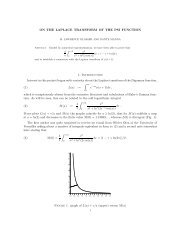
• Though the convergence rate is slower for larger a, the
method allows, say, graphing R to reasonable precision.
A plot of R
Having noted a formal expansion at a = 0, we naturally
asked for: An asymptotic form valid for large a?
• Via a typical asymptotic development, we find more,
namely a convergent expansion for all a > 1:
33

Starting with our second sech integral
∫ ∞
R(a) =
0 e−x/a sech x dx
we again use the Euler numbers and known Hurwitz-zeta
evaluations of sech-power integrals for odd powers. We
obtain a convergent series valid at least for real a > 1:
R(a) = π ( ) π
2 sec − 2 ∑ β(m + 1)
2a
m∈D + a m
= 2 ∑ (
β(k + 1) − 1 ) k
a
k≥0
Here D + denotes positive odd integers and
β(s) := 1/1 s − 1/3 s + 1/5 s − · · ·
is the Catalan primitive L-series mod 4.
34

• Remarkably, we find the leading terms for large a involve
Catalan’s constant G := β(2) via
R(a) = π 2 − 2G a +
π3
16a 2 − · · ·,
a development difficult to infer from casual inspection
of Ramanujan’s fraction.
• Even the asymptote R(∞) = π/2 is hard to so infer,
though it follows from various of the previous representations
for R(a). Using recurrence relations and
various expansions we also obtain results pertaining to
the derivatives of R, notably
)
= π2
(
R ′ (1) = 8(1 − G), R ′ 1
2 24 . 35

• A peculiar property of ψ leads to an exact evaluation
of the imaginary part of the digamma representation
of R(a) when a lies on the circle
in the complex plane.
C 1/2 := {z : |z − 1 2 | = 1 2 }
Imaginary parts of the needed digamma values have a
closed form [AS,St], and we obtain
for
Im(R(a)) = π 2 cosech ( πy
2
y := i
(
1 − 1 )
a
)
− 1 y
and a ∈ C 1/2 .
36

• Note that y is always real, and we have an elementary
form for Im(R) on the given continuum set. Admittedly
we have not yet discussed complex parameters; we do
that later.
• The Ramanujan fraction converges at least for a =
b, Re(a) ≠ 0, and it is instructive to compare numerical
evaluations of imaginary parts via the above cosech
identity.
Firmament — made for Coxeter at ninety
37

5. The R Function at Rational Arguments
For positive integers p, q, we have from the above
( ) (
p 1
R = 2p
q q + p − 1
q + 3p + 1
)
q + 5p − . . . ,
which is in the form of a Dirichlet L-function. One way to
evaluate L-functions is via Fourier-transforms to pick out
terms from a general logarithmic series. An equivalent,
elementary form for the digamma at rational arguments is
a celebrated result of Gauss. In our case
( )
p
q
⎧
⎨
R
=
4p ∑
odd k>0
⎩ − log ( 1 − e 2πi k/(4p)) − 1 n
e −2πi k(q+p)/(4p) ×
q+p−1 ∑
n=1
e 2πi kn/(4p) ⎫
⎬
⎭ . 38

After various simplifications, forcing everything to be realvalued,
we arrive at a finite closed form. Namely:
R
( p
q)
= −2p
− 2
+ 2π
p+q−1
∑
n=1
∑
1 ( )
δn≡p+q mod 4p − δ n≡3p+q mod 4p
n
0

Exact Evaluations
R(1/4) = π 2 − 4 , R(1/3) = 1 − log 2,
3
R(1) = log 2, R(1/2) = 2 − π/2,
R(2/3) = 4 − π √
2
− √ 2 log(1 + √ 2),
R(3/2) = π + √ 3 log (2 − √ 3),
R(2) = √ { π
2
2 − log(1 + √ }
2) ,
R(3) = π √
3
− log 2,
40

• And, of course, many other attractive forms.
• From (5.1) for positive integer q one has
R(1/q) = rational + (−1) (q−1)/2 log 2
(q odd)
R(1/q) = rational + (−1) q/2 π/2
(q even)
as also follow from R(1) = log 2, R(1/2) = 2−π/2 and
( )
1
R = 2
( )
1
q q − 1 − R .
q − 2
• An alluring evaluation involves the golden mean:
R(5) = √
π
τ √ + log 2 − √ 5 log τ, (τ := (1+ √ 5)/2).
5
41

• Such evaluations—based on (5.1)—can involve quite
delicate symbolic work.
• We have not analyzed evaluating R(a) for irrational a
by approximating a first via high-resolution rationals,
and then using (5.1).
Such a development would be of both computational
and theoretical interest.
42

• Armed with exact knowledge of R(p/q) we find some
interesting Gauss-fraction results, in the form of rational
multiples of
F (γ, 1; 1 + γ; −1) = [α 1 , α 2 , . . . ].
For example, (4.2) yields
R(1) = log 2 =
1 +
1
1
1
2 +
3 + 1
1 + ...
,
43

But alas the beginnings of this fraction are misleading;
subsequent elements a n run
log 2 = [1, 2, 3, 1, 5, 2 3 , 7, 1 2 , 9, 2 5 , . . . ],
being as α n = n, 4/n resp. for n odd, even.
Similarly, one can derive
2 − 2 log 2 = [1 3 , r 2 , 2 3 , r 4 , 3 3 , r 6 , 4 3 , . . . ],
are com-
where the even-indexed fraction elements r 2n
putable rationals.
• Though these RCFs do not have integer elements, the
growths of the α n provide a clue to the convergence
rate, which we study in a subsequent section.
44

6. Transformation of R 1 (a, b)
The big step. We noted that the sech-elliptic series (3.1)
(also (3.2)) will converge slowly when b ≈ a, yet in
Sections 4, 5 we successfully addressed the case b = a.
We now establish a series representation when b < a
but b is very near to a.
We employ the wonderful fact that sech is its own Fourier
transform, in that
∫ ∞
−∞ ei γx sech(λx) dx = π λ sech ( πγ
2λ
)
.
46

Using this relation, one can perform a Poisson transform
of the sech-elliptic series (3.1).
• The success of the transform depends on analyzing
I(λ, γ) :=
∫ ∞
−∞
sechλx
1 + x 2 ei γx dx.
One may obtain the differential equation:
− ∂2 I
∂γ 2 + I = π ( ) πγ
λ sech 2λ
and solve it — after some machinations.
47

We obtained
I(λ, γ) = π
cos λ e−γ + 2π λ
∑
−πd γ/(2λ)
(−1) (d−1)/2 e
d∈D + 1 − π 2 d 2 /(4λ 2 )
where D + denotes the positive odd integers.
.
• When λ = πD/2 for some odd D, the 1/ cos pole conveniently
cancels a corresponding pole in the summation,
and the result can be inferred either by avoiding d = D
in the sum and inserting a precise residual term
∆I = π(−1) (D−1)/2 e −γ (γ + 1/2)/λ,
or more simply by taking a numerical limit as λ → πD/2.
48

• When γ → 0 we can recover the ψ-function form of the
integral of sech(λx)/(1 + x 2 ).
Via Poisson transformation of (3.1) we obtain, for 0 < b < a,
( ) πa
R 1 (a, b) = R
2K ′ + π 1
cos K′ e
a
2K/a (6.1)
− 1
+ 8πa K ′ ∑ (−1) (d−1)/2 1
4K ′2 − π 2 d 2 a 2 e πd K/K′ − 1
d∈D +
where k := b/a, K := K(k), K ′ := K(k ′ ), and D + again
denotes the positive odd integers.
A similar Poisson transform obtains from (3.2) in the case
b > a > 0. Such transforms appear recondite, but we have
what we desired: convergence is rapid for b ≈ a: because
K/K ′ ∼ ∞.
49

7. Convergence Results
For an RCF x = [a 0 , a 1 , . . . ] (i.e., each a i is nonnegative but
need not be integer) one has the usual recurrence relations ∗
with
p n = a n · p n−1 + 1 · p n−2 ,
q n = a n · q n−1 + 1 · q n−2 ,
(p 0 , p −1 , q 0 , q −1 ) := (a 0 , 1, 1, 0).
∗ The corresponding matrix scheme with b n
generally to CF’s.
inserted for ‘1’ applies
50

We also have the approximation rule for the convergents
∣
∣ x − p ∣ ∣∣∣∣
n
<
q n
1
q n q n+1
,
so that convergence rates can be bounded by virtue of the
growth of the q n .
• One may iterate the recurrence in various ways, obtaining
for example
(
q n = 1 + a n a n−1 + a )
n
q n−2 −
a n
q n−4 .
a n−2 a n−2
51

An immediate application is
Theorem 7.1: For the RCF form of the Gauss fraction,
F (γ, 1; 1 + γ; −1) = [α 1 , α 2 , . . . ], and for γ > 1/2 we have
∣
∣ F − p ∣ ∣∣∣∣
n
<
q n
where c is an absolute constant.
c
8 n/2,
Remark: One can obtain sharper γ-dependent bounds.
We intend here just to show geometric convergence; i.e.
that the number of good digits grows at least linearly in
the number of iterates.
Also note that for the R(a) evaluation of current interest,
γ = 1/2 + 1/(2a) so that the condition on γ is natural.
52

Proof: From the element assignments in (4.2) we have
α n α n−1 =
4
(n − 1 + γ)(n − 2 + γ);
(n − 1) 2
1 < n odd ,
α n α n−1 =
1
(n − 1 + γ)(n − 2 + γ);
(n/2 − 1 + γ) 2
n even .
We also have q 1 = 1, q 2 = 1 + 1/γ > 2 so that for sufficiently
large n we have α n α n−1 + 1 > 4,2 respectively as n
is odd, even.
From the estimate q n > (α n α n−1 + 1)q n−2 the desired bound
follows.
c⃝
53

• A clever computational acceleration for Gauss fractions
is described in [BBa1,AAR,LW]. Consider the previously
displayed fraction log 2 = [1, 2, 3, 1, 5, 2/3, . . .].
Generally a “tail” t N of this construct, meaning a subfraction
starting from the N-th element, runs like so:
t N :=
1
.
4
N + 1
1
N + 1 +
4
N + 2 + 1
N + 3 + ...
We hope this tail t N is near the periodic fraction
[4/N, N, 4/N, N, . . . ] = N( √ 2 − 1)/2.
54

• This suggests that if we evaluate the Gauss fraction
and stop at element 4/N, this one element should be
replaced by 2(1 + √ 2)/N.
- in our own numerical experiments, this trick always
adds a few digits precision.
• As suggested in [LW], there are higher-order takes of
this idea; e.g., the use of longer periods for the tail
sub-fraction.
- as the reference shows, experimentally, the acceleration
can be significant.
55

Convergence Rates
We now attack convergence of the Ramanujan RCF, viz
a
R 1 (a, b) = [A 0; A 1 , A 2 , A 3 , . . . ].
with the A i defined subsequent to (2.1).
• The q n convergents are linear combinations of a i · b j ’s
for i, j even integers, and can be explicitly determined.
56

This leads to
q n ≥ 1 + bn−2
a n
n ∏
m even
(
1 − 1 ) 2
m
> 1 + 1
2n
b n−2
a n
q n ≥ 1 b 2 + an−1
b n+1
n−1 ∏
m even
for n even,
( m
m + 1
> 1 b 2 + 1 n
) 2
a n−1
b n+1
for n odd.
57

• We are ready for a convergence result —which can be
sharpened — for the original Ramanujan construct:
Theorem 7.2: For the Ramanujan RCF
a
R 1 (a, b) = [A 0; A 1 , A 2 , A 3 , . . .]
we have for b > a > 0
∣
a
R 1 (a, b) − p ∣ ∣∣∣∣
n
<
q n
while for a > b > 0 we have
∣
a
R 1 (a, b) − p ∣ ∣∣∣∣
n
<
q n
2nb4
(b/a) n,
nb/a
(a/b) n.
Proof: The given bounds follow directly upon inspection
of the products q n q n+1 .
c⃝
58

• As previously intimated, convergence for a = b is slow.
What we can prove is:
Theorem 7.3: For real a > 0, we have
∣
a
R(a) − p ∣ ∣∣∣∣
n
< c(a)
q n
n h(a),
where c(a), h(a) are n-independent constants.
The exponent h(a) can be taken to be
h(a) = c 0 min(1, 4π 2 /a 2 )
where the constant c 0 is absolute (can be sharpened—and
made more explicit.)
59

Remark: The bound is computationally poor, but convergence
does occur. Indeed, for a = b or even a ≈ b we now
have many other, rapidly convergent options.
Proof: Inductively, assume for (n-independent) d(a), g(a)
and n ∈ [1, N −1] that q n < dn g . The asymptotics following
(2.1) mean A n > f(a)/n for an n-independent f.
Then we have a bound for the next q N :
q N > f N d(N − 1)g + d (N − 2) g .
For g < 1, 0 < x ≤ 1/2 we have
(1 − x) g > 1 − gx − gx 2 ,
and the constants d, g can be arranged so that q N > dN g ;
hence the induction goes through.
c⃝
60

We reprise the import of these three theorems:
• (Theorem 7.1) The Gauss fraction for R(a) exhibits
(at least) geometric/linear convergence.
• (Theorem 7.2) So does the original Ramanujan form
R 1 (a, b) when a/b or b/a is (significantly) greater than
unity .
• (Theorem 7.3) When a = b we still have convergence
in the original form.
As suggested by Theorem 7.3 convergence is far below
geometric/linear.
61

8. A Uniformly Convergent Algorithm
• We now give a complete algorithm to evaluate the
original fraction R η (a, b) for positive real parameters.
• Convergence is uniform — for any positive real triple
η, a, b we obtain D good digits in no more than c D
computational iterations, where c is independent of the
size of η, a, b. ∗
∗ ‘Iterations’ mean continued-fraction recurrence steps, or seriessummand
additions.
62

Algorithm for R η (a, b) with real η, a, b > 0:
1. Observe that R η (a, b) = R 1 (a/η, b/η) so with impunity we may
assume η = 1 and evaluate only R 1 .
2. If (a/b > 2 or b/a > 2) return original (1.1), or equivalently (2.1);
3. If (a = b) {
if (a = p/q rational) return finite form (5.1); else return the Gauss
RCF (4.2) or rational-zeta form (4.1) or (4.3) or some other
scheme such as rapid ψ computations; }
4. If (b < a) {
if (b is not too close to a) ∗ , return sech-elliptic result (3.1); else
return Poisson-transform result (6.1); }
5. (We have b > a) Return, as in (1.2),
2R 1
((a + b)/2, √ )
ab − R 1 (b, a).
c⃝
∗ Say, |1 − b/a| > ε > 0 for any fixed ε > 0.
63

• It is an implicit tribute to Ramanujan’s ingenuity that
the final step (4) of the algorithm allows the entire procedure
to go through for all positive real parameters.
• One may avoid step (4) by invoking a Poisson transformation
of (3.2), but Ramanujan’s AGM identity is
finer!
64

PART II: 9. About Complex Parameters
PART II. Complex parameters a, b, η are complex, as we
found via extensive experimentation.
We attack this by assuming η = 1 and defining
D := {(a, b) ∈ C 2 : R 1 (a, b) converges},
i.e., the convergents for (1.1) have a well-defined limit.
• There are literature claims [BeIII] that
{(a, b) ∈ C 2 : Re(a), Re(b) > 0} ⊆ D,
i.e., that convergence occurs whenever both parameters
have positive real part.
65

• This is false — as we shall
show. The exact identification
of D is very delicate.
• R 1 (a, b) typically diverges for |a| = |b|: we observed numerically
∗ that
( √ 1 −3
R 1
2 + 2 , 1 √ )
−3
2 − 2
and R 1 (1, i) have ‘period two’ — as is generic — while
R 1 (t i, t i) is ‘chaotic’ for t > 0.
∗ After a caution on checking only even terms!
66

• We have implicitly used, for positive reals a ≠ b and
perforce for the Jacobian parameter
the fact that
q :=
min(a, b)
max(a, b)
0 ≤ θ 2(q)
θ 3 (q) < 1.
∈ [0, 1),
• If, however, one plots complex q with this ratio of absolute
value less than one, a complicated fractal
structure emerges, as shown in the Figures below —
this leads to the theory of modular forms [BB].
• Thence the sech relations of Theorem 2.1 are suspect
for complex q.
67

• Numerically, the identities appear to fail when |θ 2 (q)/θ 3 (q)|
exceeds unity as graphed in white for |q| < 1:
• Such fractal behaviour is ubiquitous.
68

• Where |θ 4 (q)/θ 3 (q)| > 1 in first quadrant. ∗
∗ Colours show gradations between zero and one.
69

Though the fraction R 1 (a, b)
converges widely, the AGM
relation (1.2) does not hold
across D.
Using a := 1, b := −3/2 + i/4 the computationalist will find
that the AGM relation fails:
⎛
R 1
⎝− 1 4 + i √ ⎞
8 , − 3 2 + i ⎠ ≠ R 1 (1, b) + R 1 (b, 1)
.
4
2
• The key to determining the domain for the AGM relation
seems to be the ordering of the moduli of the
relevant parameters.
70

• We take the elliptic integral K(k) for complex k to be
defined by
K(k) = π 2 F ( 1
2 , 1 2 ; 1; k2 ).
• The hypergeometric function F converges absolutely
for k in the disk (|k| < 1) and is continued analytically.
• For any numbers z = re iϕ under discussion, r ≥ 0, arg(z) ∈
(−π, +π] and so
√ z :=
√ re iϕ/2 .
• We start with some numerically based Conjectures now
proven:
71

Theorem 9.0 (Analytic continuation): Consider complex
pairs (a, b). Then
If |a| > |b| the original fraction R 1 (a, b) exists and agrees
with the sech series (3.1).
If |a| < |b| the original fraction R 1 (a, b) exists and agrees
with the sech series (3.2).
Theorem 9.1: R(a) := R 1 (a, a) converges iff a ∉ I. That
is, the fraction diverges if and only if a is pure imaginary.
Moreover, for a ∈ C\I the fraction converges to a holomorphic
function of a in the appropriate open half-plane.
Theorem 9.2: R 1 (a, b) converges for all real pairs; that is
whenever Im(a) = Im(b) = 0.
72

Theorem 9.3: (i) The even/odd parts of R 1 (1, i) (e.g.)
converge to distinct limits.
(ii) There are Re(a), Re(b) > 0 such that R 1 (a, b) diverges.
⋆ Define
• H := {z ∈ C :
• K := {z ∈ C :
2√ z
∣
1+z
2z
∣
∣ < 1},
1+z 2 ∣ ∣∣ < 1}.
Theorem 9.4: If a/b ∈ K then R 1 (a, b) and R 1 (b, a) both
converge.
Theorem 9.5: H ⊂ K (properly).
These results combine to give a region of validity for the
AGM relation:
73

Theorem 9.6: If a/b ∈ H then R 1 (a, b) & R 1 (b, a) converge,
and the arithmetic mean (a + b)/2 dominates the
geometric mean √ ab in modulus.
• As to the problematic issues regarding the AGM relation
(1.2) · · · . We performed “scatter diagram”
analysis (very robust) to find computationally where
the AGM relation held in the parameter space.
⋆ The results (shown to
the right in yellow) were
quite spectacular!
• And led to the Theorems
above.
74

• With C ′ := {z ∈ C : |z| = 1, z 2 ≠ 1}, we were led to:
Theorem 9.11:
R 1 (a, b) is
The precise domain of convergence for
D 0 = {(a, b) ∈ C × C : (a/b ∉ C ′ ) or (a 2 = b 2 , b ∉ I)}.
Hence, for a/b ∈ C ′ we have divergence. Also, R 1 (a, b) converges
to an analytic function of a or b on the domain
D 2 := {(a, b) ∈ C × C : |a/b| ̸= 1} ⊂ D 0 .
• Note, we are not harming Theorems 9.4–9.6 because
neither H nor K intersects C ′ .
• The “bifurcation” of Theorem 9.11 is very subtle.
75

Theorem 9.12: Restricting a/b ∈ H implies the truth of
the AGM relation (1.2) with all three fractions converging.
Proof: For a/b ∈ H, the ratio (a + b)/(2 √ ab) ∉ C ′ and via
9.11 we have sufficient analyticity to apply Berndt’s technique
of Part I.
c⃝
• A picturesque take on Theorems 9.4–9.6 and 9.12 is:
Equivalently, a/b belongs to the closed exterior
of ∂H, which in polar-coordinates is given by the
cardioid-knot
r 2 + (2 cos ϕ − 4)r + 1 = 0
drawn in the complex plane (r := |a/b|).
76

• a/b ∈ H: the arithmetic mean dominating the geometric
mean in modulus.
A cardioid-knot, on the (yellow) exterior of which the Ramanujan
AGM relation (1.2), (9.1) holds.
77

Proof:
A pair from Theorem 9.11 meets
1 ≤
∣
a + b
2 √ ab
2
∣
= 1 4
∣
∣
√ 1 ∣∣∣∣ 2
z + √z ,
with z := a/b. Thus, for z := re iϕ we have 4 ≤ r + 2 cos ϕ + 1/r,
which defines the exterior ∗ of the cardioid-knot curve. c⃝
• To clarify, consider the two lobes of ∂H: We fuse the
orbits of the ± instances, yielding:
√
r = 2 − cos θ ± (1 − cos θ)(3 − cos θ).
• Thus, H has a small loop around the origin, with leftintercept
√ 8 − 3 + 0i, and a wider contour whose leftintercept
is −3 − √ 8 + 0i.
∗ As determined by Jordan crossings.
78

• The condition a/b ∈ H (K) is symmetric: if a/b is in
H (K) then so is b/a, since r → 1/r leaves the polar
formula invariant.
• In particular, the AGM relation holds whenever (a, b) ∈
D and a/b lies on the exterior rays:
a
b or b a ∈ [√ 8 − 3, ∞) ∪ (∞, −3 − √ 8],
thus including all positive real pairs (a, b) as well as a
somewhat wider class.
• Similarly, the AGM relation holds for pairs (a, b) = (1, iβ)
with
±β ∈ [0, 2 − √ 3] ∪ [2 + √ 3, ∞).
79

Remark. We performed extensive numerical experiments
without faulting Theorems 9.11 and 9.12.
• Even with a = b we needed (a, a) ∈ D; recall (i, i) (also
(1, i)) provably is not in D.
The unit circle only intersects H at z = 1.
Where R exists (not yellow) and where the AGM holds (red).
z
∣ ∣
√ ∣ ∣ z ∣∣∣ ∣∣∣
∣ 2 1 + z∣ ⇒ 2
1 + z 2 < 1.
80

⋄ A key component of our proofs, actually valid in any B ∗
algebra, is:
Theorem 9.13.
complex matrices.
Let (A n ), (B n ) be sequences of k × k
Suppose that ∏ n
j=1
A j converges as n → ∞ to an invertible
limit while ∑ ∞
j=1
∥B j ∥ < ∞. Then
n∏
j=1
(A j + B j )
also converges to a finite complex matrix.
81

• Theorem 9.13 appears new even in C 1 !
⋆ It allows one to linearize nonlinear matrix recursions —
ignoring O ( 1/n 2) terms for convergence purposes.
• This is how the issue we now turn to, of the dynamics
of (t n ), arose when applied to the matrix form of the
partial fraction for R 1 :
A n =
A n +B n is linearization
{ ⎡ }}
( )
{
ab 2 n
⎤
I + 1
2an
⎢
⎣
0
( ba
) 2 n
0
⎥
⎦ −
B n
{ }} {
( ) 1
O
n 2
82

10. Visual Dynamics from a ‘Black Box’
• Six months after the discoveries we had a beautiful proof
using genuinely new dynamical results.
Starting from the linear dynamical system t 0 := t 1 := 1:
t n ←↪
1
n t n−1 + ω n−1
(1 − 1 n
)
t n−2 ,
where ω n = a 2 , b 2 for n even, odd respectively — or is much
more general.
• Indeed √ n t n is bounded ⇔ R 1 (a, b) diverges [actually
t n = q n−1 /n!]
83

• Numerically all one learns is that it is “tending to zero
slowly”. Pictorially we see significantly more:
• Scaling by √ n, and coloring odd and even iterates, fine
structure appears.
84

The attractors for various |a| = |b| = 1.
85

⋆ This is now fully explained, especially the original rate
of convergence, which follows by a fine singular-value
argument. The radii are also determined.
• We used our matrix stability theorem to show the hard
case: |a| = |b|, a ≠ b, a ≠ 0 implies divergence of the
fraction.
• A Cinderella generated applet at
http://www.carma.newcastle.edu.au/~jb616/rama.html
neatly illustrates the behaviour of t n .
♠ L. Lorentzen (2008) has now provided a fine more conventional
proof of Theorem 9.11.
86

11. The ’Chaotic’ Case
Jacobsen-Masson theory used in Theorem 9.1 shows, unlike
R 1 (1, i), even/odd fractions for R 1 (i, i) behave “chaotically,”
neither converge.
When a = b = i, (t n ) exhibit a fourfold quasi-oscillation, as
n runs through values mod 4.
⋆ Plotted versus n, the (real) sequence t n (1,1) exhibits
the “serpentine oscillation” of four separate “necklaces.”
87

For a = i, the detailed asymptotic is
√
2
t n (1, 1) =
π cosh π (
1
1
√
(1 + O ×
2 n n))
where
⎧
⎨
⎩
(−1) n/2 cos(θ − log(2n)/2)
(−1) (n+1)/2 sin(θ − log(2n)/2)
n is even
n is odd
θ := arg Γ((1 + i)/2).
88

The subtle four fold serpent.
♠ This behaviour seems very difficult to infer directly from
the recurrence.
89

♡ Analysis is based on a striking hypergeometric parametrization
which was both experimentally discovered and
computer proved!
It is
where
t n (1, 1) = 1 2 F n(a) + 1 2 F n(−a),
a n 2 1−ω
F n (a) := −
ω β(n + ω, −ω) 2 F 1
(ω, ω; n + 1 + ω; 1 2
where
and ω = 1−1/a
2
.
β(n + 1 + ω, −ω) =
Γ (n + 1)
Γ (n + 1 + ω) Γ (−ω) ,
)
,
90

12. More General Fractions
Study of R devolved to hard but compelling conjectures
on complex dynamics, with many interesting proven and
unproven generalizations (e.g., Borwein-Luke, 2008).
For any sequence a ≡ (a n ) ∞ n=1
, we considered fractions
like
S 1 (a) =
1 +
1 2 a 2 1
2 2 a 2 2
1 + 32 a 2 3
1 + . ..
91

• We studied convergence properties for deterministic
and random sequences (a n ).
• For the deterministic case the best results are for periodic
sequences, satisfying
for all j and some finite c.
a j = a j+c
• The cases (i) a n = Const ∈ C, (ii) a n = −a n+1 ∈ C, (iii)
|a 2n | = 1, a 2n+1 = i, and (iv) a 2n = a 2m , a 2n+1 = a 2m+1
with |a n | = |a m | ∀ m, n ∈ N, were already covered.
92

A period three dynamical system
(odd and even iterates)

13. Final Open Problems
• On the basis of numerical experiments, we note that
some “deeper” AGM identity might hold.
- there are pairs {a, b} so
(
R 1 (a, b) + R 1 (b, a) a + b
≠ R 1
2
2 , √ )
ab
but the LHS agrees numerically with some variant,
S 1 ((a + b)/2, √ ab), naively chosen from (3.1)
or (3.2).
- such coincidences are remarkable and difficult to
predict.
93

1. What precisely is the domain of pairs for which R 1 (a, b)
converges, and some AGM holds?
2. Relatedly, when does the fraction depart from its various
analytic representations?
3. While R(i) := R 1 (i, i) does not converge, the ψ-function
representation of Section 4 has a definite value at a = i.
Does some limit such as lim ϵ→0 R 1 (i + ϵ, i) exist and
coincide?
4. Despite a host of closed forms for R(a) := R 1 (a, a), we
know no nontrivial closed form for R 1 (a, b) with a ≠ b.
94

G.H. Hardy
All physicists and a good many quite respectable
mathematicians are contemptuous about proof.
Beauty is the first test. There is no permanent
place in the world for ugly mathematics.
Acknowledgements: Thanks are due to David Bailey,
Bruce Berndt, Joseph Buhler, Stephen Choi, William Jones,
and Lisa Lorentzen for many useful discussions.
95

14. Other References
AS Milton Abramowitz and Irene A. Stegun, Handbook of Mathematical
Functions, Dover Publications, New York, 1970.
AAR George E. Andrews, Richard Askey and Ranjan Roy, Special Functions,
Cambridge University Press, 1999.
BeII, III Bruce C. Berndt, Ramanujan’s Notebooks, Parts II & III, Springer-
Verlag, 1999.
BBa1 Jonathan M. Borwein and David H. Bailey, Mathematics by Experiment:
Plausible reasoning in the 21st century, A.K. Peters Ltd,
Ed 2, 2008.
BBa2 Jonathan M. Borwein and David H. Bailey, Experimentation in
Mathematics: Computational paths to discovery, A.K. Peters Ltd,
2004.
96

BB Jonathan M. Borwein and Peter B. Borwein, Pi and the AGM:
A study in analytic number theory and computational complexity,
CMS Series of Monographs and Advanced books in Mathematics,
John Wiley & Sons, 1987.
BBC Jonathan M. Borwein, David M. Bradley and Richard E. Crandall,
Computational strategies for the Riemann zeta function, Journal
of Computational and Applied Mathematics, 121 (2000), 247–
296.
BCP Jonathan M. Borwein, Kwok-Kwong Stephen Choi and Wilfrid
Pigulla, Continued fractions as accelerations of series, American
Mathematical Monthly, 6 (2005), 493–501.
JT W. Jones and W. Thron, Continued Fractions: Analytic Theory
and Applications, Addison–Wesley, 1980.
Kh A. Khintchine, Continued fractions, University of Chicago Press,
Chicago, 1964.
97

LL L. Lorentzen, Convergence and divergence of the Ramanujan AGM
fraction, Ramanujan J. 16 (2008), 83–95.
LW L. Lorentzen and H. Waadeland, Continued Fractions with Applications,
North-Holland, Amsterdam, 1992.
St Karl R. Stromberg, An Introduction to Classical Real Analysis,
Wadsworth, 1981.