Title : Alternate Mixed Method: Old Wine in a New Bottle - IRCC
Title : Alternate Mixed Method: Old Wine in a New Bottle - IRCC
Title : Alternate Mixed Method: Old Wine in a New Bottle - IRCC

You also want an ePaper? Increase the reach of your titles
YUMPU automatically turns print PDFs into web optimized ePapers that Google loves.
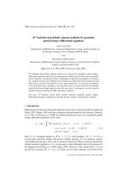
<strong>Alternate</strong> <strong>Mixed</strong> <strong>Method</strong>: <strong>Old</strong> <strong>W<strong>in</strong>e</strong> <strong>in</strong> a <strong>New</strong><br />
<strong>Bottle</strong><br />
Amiya Kumar Pani 1<br />
akp@math.iitb.ac.<strong>in</strong><br />
Industrial Mathematics Group<br />
Department of Mathematics<br />
IIT Bombay, Powai<br />
Mumbai-400 076<br />
August 17, 2011<br />
1 Collaborators: G. Fairweather, R.K.S<strong>in</strong>ha, Arul Veda Manickam ,Kannan<br />
Moudgalya, M.A. Ali and A.K. Otta<br />
1 / 37 <strong>IRCC</strong>, IITB <strong>Alternate</strong> <strong>Mixed</strong> <strong>Method</strong>
Sketch of the Talk<br />
On Computational Mathematics<br />
A new way of look<strong>in</strong>g at Mathematics<br />
Broad Focus<br />
Why <strong>Mixed</strong> <strong>Method</strong><br />
An Example <strong>in</strong> Enhanced Oil Recovery<br />
To illustrate with simpler Problem<br />
Classical <strong>Mixed</strong> <strong>Method</strong> (p, u)<br />
Formulation: What we have ga<strong>in</strong>ed & What we have lost<br />
LBB Consistency Condition<br />
Order of Convergence<br />
Disadvantages<br />
2 / 37 <strong>IRCC</strong>, IITB <strong>Alternate</strong> <strong>Mixed</strong> <strong>Method</strong>
Sketch of the Talk (contd.)<br />
Proposed <strong>Mixed</strong> <strong>Method</strong><br />
Basic Idea: symmetrization<br />
<strong>Old</strong> w<strong>in</strong>e <strong>in</strong> a new bottle : justification<br />
Order of convergence<br />
Comparision<br />
Modified <strong>Method</strong><br />
Non-conformity<br />
Improved rate of convergence<br />
Summary and Extension<br />
3 / 37 <strong>IRCC</strong>, IITB <strong>Alternate</strong> <strong>Mixed</strong> <strong>Method</strong>
On Computational Mathematics<br />
☞ When a given problem is approximated us<strong>in</strong>g a f<strong>in</strong>ite<br />
mach<strong>in</strong>e ( mach<strong>in</strong>e with a f<strong>in</strong>ite precession), we commit<br />
round off errors or truncation errors at every stage of<br />
computation.<br />
☞ It is, therefore, essential to have a control on these errors.<br />
☞ To illustrate the effect of round off or truncation error,<br />
consider solv<strong>in</strong>g<br />
AX = b, (1)<br />
where b is a given vector and A is a Hilbert matrix, which<br />
is given by<br />
1<br />
A ij =<br />
i + j − 1 .<br />
4 / 37 <strong>IRCC</strong>, IITB <strong>Alternate</strong> <strong>Mixed</strong> <strong>Method</strong>
On Computational Mathematics (contd.)<br />
In other words<br />
⎡<br />
A n×n =<br />
⎢<br />
⎣<br />
1<br />
1<br />
3<br />
· · ·<br />
n<br />
1<br />
1<br />
4<br />
· · ·<br />
n+1<br />
1<br />
1<br />
5<br />
· · ·<br />
n+2<br />
· · · · · · · · · · · · · · ·<br />
1 1 1<br />
1<br />
n n+1 n+2<br />
· · ·<br />
2n−1<br />
1<br />
1<br />
2<br />
1 1<br />
2 3<br />
1 1<br />
3 4<br />
⎤<br />
⎥<br />
⎦<br />
5 / 37 <strong>IRCC</strong>, IITB <strong>Alternate</strong> <strong>Mixed</strong> <strong>Method</strong>
On Computational Mathematics (contd.)<br />
☞ It is easy check that<br />
det A ≠ 0,<br />
and hence, the matrix A is nons<strong>in</strong>gular.<br />
☞ Therefore, (1) yields<br />
X := A −1 b. (2)<br />
☞ When you compute with f<strong>in</strong>ite mach<strong>in</strong>e: a small change <strong>in</strong><br />
b gives rise to a drastic change <strong>in</strong> the solution.<br />
☞ For example, consider<br />
b ′ = (1, 0, 0, · · · , 0) 1×50<br />
and a slight perturbation of b:<br />
˜b ′ = (1 + 10 −3 , 0, 0, · · · , 0) 1×50 .<br />
6 / 37 <strong>IRCC</strong>, IITB <strong>Alternate</strong> <strong>Mixed</strong> <strong>Method</strong>
On Computational Mathematics (contd.)<br />
☞ Now,<br />
‖b − ˜b‖ max := max<br />
1≤i≤50 |b i − ˜b i | ≤ 10 −3 .<br />
For comput<strong>in</strong>g solution of<br />
AX = b, and A˜X = ˜b,<br />
us<strong>in</strong>g a f<strong>in</strong>ite mach<strong>in</strong>e, we observe that<br />
‖X − ˜X‖ max = max<br />
1≤i≤50 |X i − ˜X i | ≤ 2.9329 × 10 6 .<br />
small chage <strong>in</strong> b gives rise to drastic change <strong>in</strong> the<br />
solution.<br />
☞ Therefore, if we use low end mach<strong>in</strong>e and then high end<br />
mach<strong>in</strong>e, there will be be a drastic change <strong>in</strong> the solution<br />
and it is not acceptable as an approximate solution.<br />
7 / 37 <strong>IRCC</strong>, IITB <strong>Alternate</strong> <strong>Mixed</strong> <strong>Method</strong>
On Computational Mathematics (contd.)<br />
☞ To probe a bit: it is the effect of round off error.<br />
Therefore, a new way of look<strong>in</strong>g at Mathematics<br />
has emerged <strong>in</strong> the last fifty or sixty<br />
years. A part from Pure and Applied Mathematics,<br />
now a new branch called ‘Computational<br />
Mathematics’ has developed.<br />
☞ In this talk, we concentrate on ’Computational PDEs’.<br />
8 / 37 <strong>IRCC</strong>, IITB <strong>Alternate</strong> <strong>Mixed</strong> <strong>Method</strong>
Computational PDEs<br />
Broad Focus:<br />
To provide mathematical justifications <strong>in</strong> terms of<br />
stability and convergence to widely used numerical<br />
schemes for computational PDEs.<br />
To design and develop reliable and efficient algorithms<br />
for numerical solutions to PDEs.<br />
By reliability, we mean that for a given tolerance and<br />
measurement, the computed solution stays near to the<br />
exact unknown solution that too with<strong>in</strong> the prescribed<br />
tolerance with respect to the given measurement.<br />
By efficient, we understand that this can be achieved with<br />
m<strong>in</strong>imal computational effort.<br />
Theme of this talk: propose a new method with proper<br />
mathematical justifications.<br />
9 / 37 <strong>IRCC</strong>, IITB <strong>Alternate</strong> <strong>Mixed</strong> <strong>Method</strong>
To motivate through an example from Enhanced Oil<br />
Recovery<br />
In tertiary oil recovery an <strong>in</strong>expensible fluid is <strong>in</strong>jected <strong>in</strong>to the<br />
reservoir to mix with the hydrocarbon (Oil) and then push the<br />
mixture towards the production wells.<br />
10 / 37 <strong>IRCC</strong>, IITB <strong>Alternate</strong> <strong>Mixed</strong> <strong>Method</strong>
Enhanced Oil Recovery (contd.)<br />
Assum<strong>in</strong>g that there is no volume change due to mix<strong>in</strong>g and the<br />
fluid is slightly compressible , the mathematical model gives<br />
rise to the follow<strong>in</strong>g system of PDEs:<br />
For a given T > 0, f<strong>in</strong>d a pair (p,c) such that<br />
✓<br />
d(c) ∂p<br />
∂t<br />
− ∇.(a(c)∇p) = q, (x, t) ∈ Ω × J<br />
φc t + b(c) ∂p<br />
✒<br />
∂t<br />
+ u.∇c − ∇.(D(u)∇c) = g(c)<br />
with no flow boundary conditions and <strong>in</strong>itial condition<br />
✏<br />
✑<br />
p(x, 0) = p 0 (x), c(x, 0) = c 0 (x), x ∈ I.<br />
11 / 37 <strong>IRCC</strong>, IITB <strong>Alternate</strong> <strong>Mixed</strong> <strong>Method</strong>
Enhanced Oil Recovery (contd.)<br />
• Ω is a bounded doma<strong>in</strong> <strong>in</strong> IR 2 , J = (0, T ).<br />
• u is the Darcy velocity,<br />
u = −(a(c)∇p).<br />
• a(c) = k(x)<br />
µ(c)<br />
, k(x)- the permeability, µ(c) - viscosity.<br />
• φ -the porosity<br />
• q is the total external flow.<br />
• D = D(x, u) is diffusion coefficient.<br />
• ˜c is a function specified at <strong>in</strong>jection po<strong>in</strong>t and equals to c at<br />
production po<strong>in</strong>t, c = c 1 = 1 − c 2 , where c 1 and c 2 is the<br />
concentrations of the two fluid components, 0 ≤ c ≤ 1.<br />
• g(c) = (c − ˜c)q,<br />
• c 0 (x) is a function must be specified.<br />
12 / 37 <strong>IRCC</strong>, IITB <strong>Alternate</strong> <strong>Mixed</strong> <strong>Method</strong>
Quantity of Interest<br />
Quantity of Interest: Concentration c<br />
(as more accurate evaluation of c is related<br />
to ‘How much oil (hydrocarbon) can<br />
be extracted from the Reservoir’)<br />
☞ For accurate evaluation of concentration c, we need more<br />
accurate evaluation of u as u not p appears <strong>in</strong> the<br />
concentration equation.<br />
Rule of the game: consider both p and u as primary<br />
variables,that is, comute both simultaneously.<br />
13 / 37 <strong>IRCC</strong>, IITB <strong>Alternate</strong> <strong>Mixed</strong> <strong>Method</strong>
To illustrate with Simpler Problem<br />
F<strong>in</strong>d p on Ω × (0, T ] such that p satisfies<br />
✗<br />
✔<br />
p t − ∇ · (a(x)∇p) = f (x, t), (x, t) ∈ Ω × J, (3)<br />
✖<br />
p = 0, (x, t) ∈ ∂Ω × J,<br />
p(x, 0) = p 0 , x ∈ Ω.<br />
Ω be a bounded doma<strong>in</strong> <strong>in</strong> R d , d = 2, 3 with smooth<br />
boundary ∂Ω.<br />
a ≥ a 0 > 0<br />
p t = ∂p<br />
∂t<br />
and J = (0, T ] with T < ∞.<br />
✕<br />
14 / 37 <strong>IRCC</strong>, IITB <strong>Alternate</strong> <strong>Mixed</strong> <strong>Method</strong>
Why <strong>Mixed</strong> <strong>Method</strong>s ?<br />
☞ To approximate p (temperature distribution) and its flux<br />
(heat flux) u = −a ▽ p through standard numerical<br />
procedures (FDM or FEM):<br />
Compute an approximation to p that is say p h .<br />
Post-process it to obta<strong>in</strong> an approximation to u that is<br />
u h = a ▽ p h .<br />
☞ Outcome: Inaccurate approximation to u.<br />
(due to numerical differentiation or/and multiplication by<br />
rough coefficient a).<br />
15 / 37 <strong>IRCC</strong>, IITB <strong>Alternate</strong> <strong>Mixed</strong> <strong>Method</strong>
Objective of <strong>Mixed</strong> <strong>Method</strong>s.<br />
☞ Reformulate the problem with both p and u as primary<br />
variables.<br />
☞ Split (3) as a system ✓<br />
✒<br />
with p(x, 0) = p 0 .<br />
αu = ∇p, α = 1 a ,<br />
∂p<br />
∂t<br />
− ∇ · u = f .<br />
✏<br />
✑<br />
☞ Weak Formulation. Let V = L 2 (Ω) : space of squre<br />
<strong>in</strong>tegrable functions, and<br />
{<br />
}<br />
W = H(div, Ω) = w : w ∈ (L 2 (Ω)) d , ∇ · w ∈ L 2 (Ω)<br />
with norm<br />
‖w‖ H(div,Ω) = (‖w‖ 2 + ‖∇ · w‖ 2 ) 1/2 .<br />
16 / 37 <strong>IRCC</strong>, IITB <strong>Alternate</strong> <strong>Mixed</strong> <strong>Method</strong>
Weak Formulation<br />
F<strong>in</strong>d (p, u) : (0, T ] ↦→ V × W such that<br />
(αu, w) + (∇ · w, p) = 0, w ∈ W,<br />
( ∂p<br />
∂t<br />
, v) − (∇ · u, v) = (f , v), v ∈ V . (2b)<br />
(2a)<br />
Galerk<strong>in</strong> Procedure. Choose the f<strong>in</strong>ite element spaces V h of<br />
V and W h of W . Seek a pair (p h , u h ) : (0, T ] ↦→ V h × W h such<br />
that<br />
(αu h , w h ) + (∇ · w h , p h ) = 0, w h ∈ W h ,<br />
( ∂p h<br />
∂t<br />
, v h ) − (∇ · u h , v h ) = (f , v h ), v h ∈ V h .<br />
17 / 37 <strong>IRCC</strong>, IITB <strong>Alternate</strong> <strong>Mixed</strong> <strong>Method</strong>
Error Analysis.<br />
☞ LBB Consistency Condition: to compensate nonsymmetric<br />
(v h ,∇·w h )<br />
sup<br />
‖w h ‖<br />
≥ β‖v<br />
H(div;Ω)<br />
h ‖ V , v ∈ V h .<br />
w h ∈ W h /{0}<br />
☞ Restriction on the construction of f<strong>in</strong>ite dimensional<br />
subspaces V h and W h .<br />
∇ · W h = V h<br />
18 / 37 <strong>IRCC</strong>, IITB <strong>Alternate</strong> <strong>Mixed</strong> <strong>Method</strong>
Raviart-Thomas-Nedelec Spaces.<br />
T h : quasi-uniform triangulation of Ω (assum<strong>in</strong>g Ω is a polygon)<br />
by triangles K of diameter at most h.<br />
19 / 37 <strong>IRCC</strong>, IITB <strong>Alternate</strong> <strong>Mixed</strong> <strong>Method</strong>
Raviart-Thomas-Nedelec Spaces.<br />
☞ Now V h = {v h ∈ V : v h | K ∈ P r−1 (K ), K ∈ T h }.<br />
☞ P j - a polynomial of degree at most j.<br />
☞ Approximation property: <strong>in</strong>f vh ∈V h<br />
‖v − v h ‖ ≤ Ch r ‖v‖ r .<br />
☞ For W h , set Q(K ) = [P r−1 ] 2 ⊕ Span(xP r−1 (K ))<br />
(space of <strong>in</strong>complete polynomials ly<strong>in</strong>g <strong>in</strong> between P r and<br />
P r−1 ) and def<strong>in</strong>e<br />
W h = {w h ∈ H(div, Ω) : w h | K ∈ Q(K ), K ∈ T h }.<br />
☞ Approximation property: <strong>in</strong>f wh ∈W h<br />
‖w − w h ‖ ≤ Ch r ‖w‖ r .<br />
☞ This construction preserves the relation<br />
∇ · W h = V h .<br />
20 / 37 <strong>IRCC</strong>, IITB <strong>Alternate</strong> <strong>Mixed</strong> <strong>Method</strong>
Convergence.<br />
For example: when r = 1<br />
V h = {v ∈ L 2 : v| K ∈ P 0 (K ), K ∈ T h }.<br />
and<br />
W h = {w ∈ H(div; Ω) : w| K = (a 1,K +b K x 1 , a 2,K +b K x 2 ) K ∈ T h }.<br />
(Johnson & Thomeé , RAIRO 1981)<br />
‖(p h − p)(t)‖ ≤ Ch r {‖p(t)‖ r + ∫ t<br />
0 ‖p t(τ)‖ r dτ}<br />
‖(u h − u)(t)‖ ≤ Ch r {‖p(t)‖ r+1 + ∫ t<br />
0 ‖p t(τ)‖ r dτ}<br />
For r = 1: Order of Convergence is One<br />
21 / 37 <strong>IRCC</strong>, IITB <strong>Alternate</strong> <strong>Mixed</strong> <strong>Method</strong>
Disadvantages.<br />
❶ Due to quasi-uniformity condition, there is difficulty <strong>in</strong><br />
apply<strong>in</strong>g adaptive methods.<br />
❷ LBB consistency condition must be satisfied, and this<br />
imposes severe restriction on the construction of f<strong>in</strong>ite<br />
element spaces<br />
❸ Computationally more simple and attractive C 0 -piecewise<br />
l<strong>in</strong>ear spaces to approximate both of p and u can not be<br />
used.<br />
22 / 37 <strong>IRCC</strong>, IITB <strong>Alternate</strong> <strong>Mixed</strong> <strong>Method</strong>
<strong>Alternate</strong> <strong>Method</strong>.<br />
☞ Attempts <strong>in</strong> the Past. (Specially for Elliptic Problems)<br />
Use of some short of stabilizers (computationally more<br />
complex and time consum<strong>in</strong>g). In fact, LBB-condition can<br />
be thought of as a stabilizer.<br />
☞ Ma<strong>in</strong> Culprit. Non-symmetric form of<br />
(∇ · w h , p h ), (∇ · u h , v h ).<br />
☞ Possible Remedy: Try to symmetrize.<br />
To provide an answer to the 14th open problem cited <strong>in</strong> a<br />
workshop on Free and Mov<strong>in</strong>g Boundary Problems held <strong>in</strong><br />
Berl<strong>in</strong> (1977), a k<strong>in</strong>d of symmetrization technique is used<br />
by us for one phase unidimensional Stefan problem (Pani<br />
and Das, IMA J. Numer. Anal. 1989, 1991,...)<br />
Spurt of Activities around 1993 for elliptic problems us<strong>in</strong>g<br />
Least Square <strong>Method</strong>.<br />
23 / 37 <strong>IRCC</strong>, IITB <strong>Alternate</strong> <strong>Mixed</strong> <strong>Method</strong>
Proposed Scheme<br />
☞ Split (3) as two first order system<br />
☞ Try to symmetrize.<br />
u = a∇p,<br />
p t − ∇·u = f .<br />
(4a)<br />
(4b)<br />
☞ Mulptiply (4a) by ∇v and (4b) by ∇ · w. Then <strong>in</strong>tegrate over<br />
Ω. Write (p t , ∇ · w) = −(∇p t , w) = −(αu t , w), where<br />
α = 1/a.<br />
☞ Weak Formulation. F<strong>in</strong>d a pair {p, u} : J ↦→ H 1 0 × W<br />
satisfy<strong>in</strong>g for w ∈ W<br />
(a∇p, ∇v) = (u, ∇v) , v ∈ H 1 0 , (5a)<br />
(αu t , w) + (∇·u, ∇·w) = − (f , ∇·w) .(5b)<br />
24 / 37 <strong>IRCC</strong>, IITB <strong>Alternate</strong> <strong>Mixed</strong> <strong>Method</strong>
Galerk<strong>in</strong> Approximation.<br />
☞ For all K ∈ T h<br />
V h = { v h ∈ C 0 (Ω) : v h | K ∈ P k (K ), v h = 0 on ∂Ω }<br />
W h = {q h ∈ W : (q h ) i | K ∈ P r (K ), i = 1, · · · , d}<br />
☞ Approximation property:<br />
<strong>in</strong>f vh ∈V h<br />
‖v − v h ‖ + h‖∇(v − v h )‖ ≤ Ch k+1 ‖v‖ k+1 .<br />
<strong>in</strong>f wh ∈W h<br />
‖w − w h ‖ + h‖∇(w − w h )‖ ≤ Ch r+1 ‖v‖ r+1 .<br />
☞ Determ<strong>in</strong>e a pair {p h , u h } : J ↦→ V h × W h satisfy<strong>in</strong>g for<br />
w h ∈ W h<br />
(a∇p h , ∇v h ) = (u h , ∇v h ) , v h ∈ V h , (6a)<br />
(αu ht , w h ) + (∇·u h , ∇·w h ) = − (f , ∇·w h ) (6b)<br />
25 / 37 <strong>IRCC</strong>, IITB <strong>Alternate</strong> <strong>Mixed</strong> <strong>Method</strong>
Semidiscrete Error Estimates.<br />
with appropriately chosen <strong>in</strong>itial pair {p h (0), u h (0)} to be<br />
def<strong>in</strong>ed later.<br />
Theorem<br />
With u 0 = a∇p 0 , assume that<br />
‖u 0 − u 0h ‖ H(div,Ω) ≤ Ch r ‖u 0 ‖ r+1 .<br />
Then there is a constant C <strong>in</strong>dependent of h such that<br />
‖∇(p − p h )(t)‖ + ‖∇ · (u − u h )(t)‖ ≤ C(u, p) h m<strong>in</strong>(r,k) ,<br />
‖(p − p h )(t)‖ + ‖(u − u h )(t)‖ ≤ C(u, p) h m<strong>in</strong>(r,k+1) .<br />
26 / 37 <strong>IRCC</strong>, IITB <strong>Alternate</strong> <strong>Mixed</strong> <strong>Method</strong>
Remark.<br />
✍ For k = r, the error estimate ‖∇ · (u − u h )(t)‖ is optimal.<br />
However, the rate of convergence <strong>in</strong> L 2 -norm is not<br />
optimal. This is due to the presence of ∇ · ρ term <strong>in</strong> the<br />
right hand side of (8b). It is possible to choose the auxiliary<br />
projection ũ I through<br />
(∇ · (u − ũ I ), ∇ · w h ) = 0, w h ∈ W h ,<br />
so that the term conta<strong>in</strong><strong>in</strong>g ∇ · ρ is zero. But it is not<br />
possible to obta<strong>in</strong> optimal L 2 -estimate for ρ t term.<br />
27 / 37 <strong>IRCC</strong>, IITB <strong>Alternate</strong> <strong>Mixed</strong> <strong>Method</strong>
☞ Note that Aub<strong>in</strong>-Nitsche duality argument requires the<br />
follow<strong>in</strong>g regularity result<br />
‖Φ‖ 2 ≤ C‖g‖<br />
(∗)<br />
for the associated operator equation<br />
☞ This may not be true. But for<br />
∇(∇ · Φ) = g.<br />
−∆Φ = ∇ × ∇ × Φ − ∇(∇ · Φ)<br />
the regularity condition (*) holds.<br />
Question:<br />
‘Is it possible to modify the formulation<br />
so that an additional term ∇ × ∇ × Φ<br />
is <strong>in</strong>troduced?’<br />
28 / 37 <strong>IRCC</strong>, IITB <strong>Alternate</strong> <strong>Mixed</strong> <strong>Method</strong>
Modified <strong>Method</strong><br />
☞ Observe that ∇ × (∇φ) = 0.<br />
☞ Rewrite (1) as<br />
p t − ∇·u = f , (x, t) ∈ Ω × J,<br />
∇ × (αu) = 0, (x, t) ∈ Ω × J, (αu = ∇p),<br />
(n ∧ αu) = 0, (x, t) ∈ ∂Ω × J, p(0) = p 0 ,<br />
n - the outward normal<br />
∧ - exterior product.<br />
☞ Weak Formulation: Let<br />
W = {w ∈ (H 1 ) d : n ∧ w = 0 on ∂Ω, d = 2, 3}.<br />
Seek a pair {p, u} : J −→ H0 1 × W such that<br />
(∇p, ∇v) = (αu, ∇v), v ∈ H0 1,<br />
(8a)<br />
(αu t , w) + A(u, w) = −(f , ∇ · w), w ∈ (H 1 ) d , (8b)<br />
where<br />
A(φ, w) = (∇ · φ, ∇ · w) + (∇ × αφ, ∇ × αw).<br />
29 / 37 <strong>IRCC</strong>, IITB <strong>Alternate</strong> <strong>Mixed</strong> <strong>Method</strong>
Galerk<strong>in</strong> Formulation.<br />
☞ A(·, ·) satisfies the coercivity condition<br />
A(φ, φ ≥ µ 0 ‖φ‖ 2 1 ,<br />
for some positive constant µ 0 , [refer to Naittaanmäki and<br />
Saranen (1981)].<br />
☞ Galerk<strong>in</strong> Formulation. V h is def<strong>in</strong>ed earlier.<br />
W h = {w h ∈ C(¯Ω) d : (w h ) i | K ∈ P r (K ), i = 1, · · · , d,<br />
(n ∧ αw h ) = 0, at the nodes on ∂Ω}.<br />
S<strong>in</strong>ce (n ∧ αw h ) = 0 only at the boundary nodes,<br />
W h ⊂ W,(non-conform<strong>in</strong>g method).<br />
☞ Determ<strong>in</strong>e a pair {p h , u h } ∈ V h × W h such that w h ∈ W h ,<br />
(∇p h , ∇v h ) = (αu h , ∇v h ), v ∈ V h ,<br />
(9a)<br />
(αu ht , w h ) + A(u h , w h ) = −(f , ∇ · w h ), (9b)<br />
30 / 37 <strong>IRCC</strong>, IITB <strong>Alternate</strong> <strong>Mixed</strong> <strong>Method</strong>
Error Analysis<br />
Theorem (Theorem 2)<br />
Assume that u h (0) = ũ h (0) with u(0) = a∇p 0 . Then, there<br />
exists a positive constant C <strong>in</strong>dependent of h such that<br />
‖(p − p h )(t)‖ + ‖(u − u h )(t)‖ + h‖(p − p)(t)‖ 1 ≤<br />
‖(u − u h )(t)‖ 1<br />
]<br />
≤<br />
Ch m<strong>in</strong>(k+1,r+1)<br />
Ch<br />
r<br />
31 / 37 <strong>IRCC</strong>, IITB <strong>Alternate</strong> <strong>Mixed</strong> <strong>Method</strong>
Remarks.<br />
1 With k = r we have<br />
‖p − p h ‖ L ∞ (L 2 ) + ‖u − u h ‖ L ∞ ((L 2 ) d ) = O(hr+1 ).<br />
2 Compared to Johnson and Thomeé [1981] the present<br />
analysis yields better results for L 2 -estimate of u − u h with<br />
higher regularity assumption on the exact solution. Further,<br />
‖u − u h ‖ = O(h r+1 ) even if k ≠ r with k < r.<br />
3 When d = 2 that is Ω ⊂ R 2 and u h (0) = ũ h (0), then us<strong>in</strong>g<br />
Sobolev imbedd<strong>in</strong>g theorem and superconvergence<br />
estimates for the ∇ζ and ∇ξ, we have the follow<strong>in</strong>g<br />
maximum norm estimates<br />
‖(p − p h )(t)‖ L ∞ ≤ C(log 1 h )hm<strong>in</strong>(k+1,r+1)<br />
provided we assume quasi-uniform condition on the f<strong>in</strong>ite<br />
element mesh.<br />
32 / 37 <strong>IRCC</strong>, IITB <strong>Alternate</strong> <strong>Mixed</strong> <strong>Method</strong>
Summary & Conclud<strong>in</strong>g Remarks<br />
✌ The Galerk<strong>in</strong> approximation has the same rate of<br />
convergence as <strong>in</strong> the case of classical mixed f<strong>in</strong>ite<br />
element method, but without LBB consistency condition<br />
and also without quasiuniform assumption on the f<strong>in</strong>ite<br />
element mesh.<br />
✌ S<strong>in</strong>ce the estimate for ‖u − u h ‖ is not optimal <strong>in</strong> two- and<br />
three space dimensions, a modification is proposed and<br />
analyzed to derive sharper estimate <strong>in</strong> L 2 -norm.<br />
33 / 37 <strong>IRCC</strong>, IITB <strong>Alternate</strong> <strong>Mixed</strong> <strong>Method</strong>
Contd.<br />
✌ Compared to classical classical mixed method, the present<br />
method allows to use two different f<strong>in</strong>ite element spaces for<br />
approximat<strong>in</strong>g p and its flux u. In particular, use of<br />
piecewise l<strong>in</strong>ear polynomial spaces yields O(h 2 ) order of<br />
convergence <strong>in</strong> both p − p h and u − u h <strong>in</strong> L 2 − norm.<br />
Although higher regularity on the solution is assumed, but<br />
better convergence results are proved specially for the flux.<br />
34 / 37 <strong>IRCC</strong>, IITB <strong>Alternate</strong> <strong>Mixed</strong> <strong>Method</strong>
Contd.<br />
Our major results:<br />
✍ Amiya K. Pani (1998),Parabolic equation with non-self<br />
adjo<strong>in</strong>t elliptic part, SIAM J. Numer. Anal. 35, pp.712–727.<br />
✍ Amiya K. Pani and Gareme Fairweather (2002),<br />
H 1 -Galerk<strong>in</strong> mixed f<strong>in</strong>ite element methods for parabolic<br />
<strong>in</strong>tegro-differential equations, IMA J. Numer. Anal. 22, pp.<br />
231–252.<br />
✍ Amiya K. Pani and Graeme Fairweather (2002), An<br />
H 1 -Galerk<strong>in</strong> mixed f<strong>in</strong>ite element method for an evolution<br />
equation with a positive type memory term, SIAM J.<br />
Numer. Anal. 40, pp. 1475–1490.<br />
35 / 37 <strong>IRCC</strong>, IITB <strong>Alternate</strong> <strong>Mixed</strong> <strong>Method</strong>
Contd.<br />
✎ Rajen K. S<strong>in</strong>ha, Ajay K. Otta and Amiya K. Pani (2004), An<br />
H 1 -Galerk<strong>in</strong> mixed method for second order hyperbolic<br />
equations, International J. Numer. Anal and Model<strong>in</strong>g, 1,<br />
pp. 111-130.<br />
✎ S. Arul Veda Manickam, Kannan M. Moudgalya and A. K.<br />
Pani (2004), Higher order fully discrete scheme comb<strong>in</strong>ed<br />
with H 1 -Galerk<strong>in</strong> mixed f<strong>in</strong>ite element method for<br />
semil<strong>in</strong>ear reaction-diffusion equations, J. Applied<br />
Mathematics and Comput<strong>in</strong>g, 15, pp. 1-28.<br />
✎ M. A. Mohamed Ali, Ph.D. dissertation on ‘Numerical<br />
<strong>Method</strong>s for Enhanced Oil Recovery <strong>in</strong> Reservoir Studies’,<br />
August ’97.<br />
36 / 37 <strong>IRCC</strong>, IITB <strong>Alternate</strong> <strong>Mixed</strong> <strong>Method</strong>
THANK YOU<br />
37 / 37 <strong>IRCC</strong>, IITB <strong>Alternate</strong> <strong>Mixed</strong> <strong>Method</strong>