2-5 Constant Acceleration and Equations of Motion

Constant Acceleration and Equations of Motion 

http://edugen.wiley.com/edugen/courses/crs1354/pc/c02/content/touger8730c02_2_5.xform?c... 

Page 1 of 6 

8/22/2006 

2-5 Constant Acceleration and Equations of Motion 

Constant Acceleration If an object's acceleration is constant, or uniform, its value never changes, so the 

instantaneous and average accelerations are the same. In that case, as in Figure 2-12, a graph of v versus t is a straight line, 

that is, its slope is the same everywhere. 

Graphing Uniformly Accelerated Motion For constant acceleration, Equation 2-7 becomes 

Proceeding as we did to obtain Equation 2-6, we call the velocity v o at t = 0, and let v be its velocity at any later instant t. 

Then 

Solving for v in 

gives us 

(2-9) 

In words: velocity at time t = initial velocity + change in velocity due to acceleration during the interval (t − 0). 

This has the general form y = b + mx or y = y o + mx of a straight line equation; t and v are the horizontally and vertically 

plotted variables, v o is the initial value of the latter—that is, the vertical intercept—and a is the rate of change or slope. To 

see how you can use this to interpret a graph of v versus t, let's work through Example 2-6. 

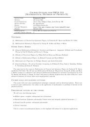
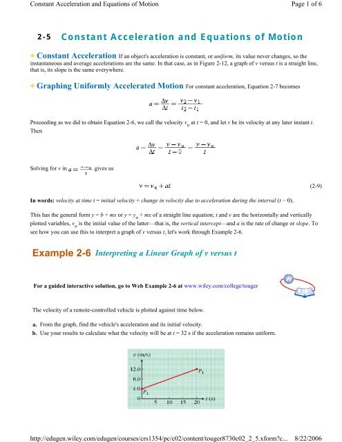
Example 2-6 Interpreting a Linear Graph of v versus t 

For a guided interactive solution, go to Web Example 2-6 at www.wiley.com/college/touger 

The velocity of a remote-controlled vehicle is plotted against time below. 

a. From the graph, find the vehicle's acceleration and its initial velocity. 

b. Use your results to calculate what the velocity will be at t = 32 s if the acceleration remains uniform.




8/22/2006 

Brief Solution 

Choice of approach. Note that v = v o + at has the same form as y = y o + mx. 

a. Slope and intercept: We can read the vertical intercept directly off the graph (point P 1 ). This is the initial velocity: v o 

= 4 m/s. 

The acceleration is the slope of the graph, which we can find from any two points on the line. In the given graph, we 

arbitrarily select points 

Thus, 

b. Equation of motion: Once we know v o and a, we can use Equation 2-9 to find v at any value of t. Thus, 

Note that both terms, v o and at, have units of velocity. 

Related homework: Problem 2-30. 

Average Velocity Suppose an object accelerates uniformly from a velocity v o at t = 0 to a velocity v at some 

later instant t. The average velocity over this interval will then be midway between the values of v o and v. In other words, it 

is the numerical average of these two values: 

(2-10) 

It is important to realize that this is generally not true when the acceleration is not uniform. Figure 2-15 shows this: in graph 

ii, the velocity is below 

for most of the interval from 0 to t, so its time-averaged value is lower. For graph iii, by 

similar reasoning, the average velocity is higher than .




8/22/2006 

Figure 2-15 Average velocities for cases of uniform and nonuniform motion. 

Before solving problems about uniformly accelerated bodies, we should first ask where in the real world do we find bodies 

experiencing constant acceleration? We will have more to say about the conditions needed for constant acceleration in 

Chapters 4 and 5, when we discuss how objects affect one another's motions. For now, we won't try to generalize. We 

simply acknowledge that there is constant acceleration when measurements show that there is, and we give examples of this 

occurring. 

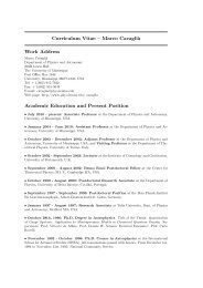
Range Finder Measurements One way of doing the necessary measurements is with a sonic range finder 

(or motion detector) connected to a computer (Figure 2-16). Software loaded into the computer enables it to do calculations 

and plot graphs using the input from the range finder. The range finder emits ultrasound pulses that travel at constant speed. 

It determines how far away a body is by sending out a pulse, detecting the pulse reflected back from the body, and timing 

the duration of the round trip. One common model makes 15 such measurements each second, so that for a moving body, 

displacements ∆x can be calculated for tiny intervals ∆t, which are measured by the computer's internal clock. Then, using 

, the software directs the computer to calculate values of average velocities that are approximately instantaneous 

because the intervals are so small. From these values, the computer can therefore use to calculate acceleration 

values that are likewise approximately instantaneous. Using these simple equations (which do not require a to be uniform) 

to do hundreds of calculations each second, the computer can find x, v, and a at successive clock readings t, and it can 

display the results as graphs. 

Figure 2-16 Range finder set-up for motion measurements. 

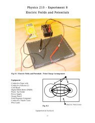
Figure 2-17 shows two situations for which these measurements are easily done. In 2-17a, the hand gives the block a shove 

to the right and the detector is turned on (t = 0) as soon as the block leaves the hand. In 2-17b, the detector is turned on 

when the weight strung over the pulley begins to fall. Figure 2-18 shows the resulting graphs. (Compare the x versus t plots 

with the graphs for cars B and C in Figure 2-8.) The v versus t graphs have constant slope, so the acceleration is 

uniform. The a versus t plots reinforce this point: They are horizontal—the value of a is not going up or down.




8/22/2006 

Figure 2-17 Making measurements on the motion of a block with a range finder. 

Figure 2-18 Motion graphs for the blocks in Figure 2-17. 

Recall that the v versus t graphs (in Figure 2-12) for the carts in Figure 2-13 are also straight lines, so the carts' 

accelerations are also constant. In short, there are a variety of situations that we can treat as having constant or roughly 

constant acceleration. 

Example 2-7 A Racing Car Speeds Up 

A racing car goes from 30 m/s to 50 m/s over a 5.0-s interval. If the acceleration is constant, how far does it go during this 

time? 

Solution 

Restating the problem. The question asks for a distance traveled during a time interval: What is |∆x| during a particular ∆t




8/22/2006 

of 5 s if v changes from v 1 = 30 m/s to v 2 = 50 m/s during this time interval? 

What we know/what we don't. 

Choice of approach. (1) Because the acceleration is constant, the average velocity meets the condition that , 

which we can use to find v . (2) Once we know v , we can use the definition of average velocity 

to find ∆x. 

The mathematical solution. 

1. 

2. Since . 

Related homework: Problems 2-35, 2-36, and 2-37. 

Completely Describing Motion from Initial Conditions Suppose an object starts out at t = 0 

with a certain initial velocity v o , and it has an acceleration a, which we know is constant. From the definition of 

acceleration, we obtained Equation 2-9, which can tell us the velocity v of the object at each subsequent instant t (see 

Example 2-6b). To describe the object's motion completely, we would need to know not only its velocity but its position x 

(or its displacement x − x o ) at each instant. To find an expression that tells us this, we can reason algebraically from 

definitions and the condition for constant acceleration. 

The definition of average velocity (Equation 2-3) now becomes 

, so that 

But 

(Equation 2-10), so 

Because we have previously found that v = v o + at, we can use this to substitute for v: 

Simplifying the right-hand side, we get 

(2-11) 

If we know the initial values (x o , v o , and an a that doesn't change), we can use this equation to find the object's position x at 

any later instant t.




8/22/2006 

Compare Equation 2-11 with x − x o = vt, which is valid whenever v is constant. If v does not change from its initial value 

v o , then a, its rate of change, is zero, and Equation 2-11 reduces to x − x o = v o t. Otherwise, the last term on the right-hand 

side of Equation 2-11 represents an additional contribution to the position. This contribution is needed because the velocity 

is changing. 

In describing a body's motion, you may also wish to find its velocity at each position x, without having to know t. To obtain 

an equation that does this, we start with what we already know and do some algebra: 

With these substitutions, we get 

For simplicity, we next solve for v 2 rather than v, obtaining 

(2-12) 

Note that solving for v would then give you 

that is, you get both positive and negative values of v. For a situation like the one in Figure 2-13b, both values are 

meaningful because the cart will pass a position x once on its way up and again on its way down. 

Copyright © 2004 by John Wiley & Sons, Inc. or related companies. All rights reserved.

2-5 Constant Acceleration and Equations of Motion

Create successful ePaper yourself

Delete template?

Save as template?