Scatter Diagrams Correlation Classifications Correlation ... - Statistics
Scatter Diagrams Correlation Classifications Correlation ... - Statistics
Scatter Diagrams Correlation Classifications Correlation ... - Statistics

Create successful ePaper yourself
Turn your PDF publications into a flip-book with our unique Google optimized e-Paper software.
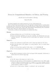
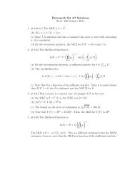
<strong>Scatter</strong> <strong>Diagrams</strong><br />
<strong>Correlation</strong> <strong>Classifications</strong><br />
• <strong>Scatter</strong> diagrams are used<br />
to demonstrate<br />
correlation between two<br />
quantitative variables.<br />
• Often, this correlation is<br />
linear.<br />
• This means that a straight<br />
line model can be<br />
developed.<br />
Weight<br />
19<br />
18<br />
17<br />
16<br />
15<br />
14<br />
13<br />
12<br />
20<br />
21<br />
22<br />
Length<br />
23<br />
24<br />
• <strong>Correlation</strong> can be<br />
classified into three basic<br />
categories<br />
• Linear<br />
• Nonlinear<br />
• No correlation<br />
Weight<br />
19<br />
18<br />
17<br />
16<br />
15<br />
14<br />
13<br />
12<br />
20<br />
Regression Plot<br />
21<br />
22<br />
23<br />
Length<br />
24<br />
Chapter 5 # 1<br />
Chapter 5 # 2<br />
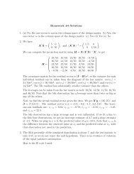
<strong>Correlation</strong> <strong>Classifications</strong><br />
<strong>Correlation</strong> <strong>Classifications</strong><br />
• Two variables may be<br />
correlated but not through<br />
a linear model.<br />
• This type of model is<br />
called non-linear<br />
• The model might be one<br />
100<br />
of a curve.<br />
0<br />
0<br />
5<br />
10<br />
15<br />
result<br />
500<br />
400<br />
300<br />
200<br />
Curvilinear <strong>Correlation</strong><br />
sample<br />
• Two quantitative<br />
variables may not be<br />
correlated at all<br />
C4<br />
50<br />
40<br />
30<br />
20<br />
10<br />
0<br />
-10<br />
-20<br />
-30<br />
-40<br />
0<br />
5<br />
10<br />
15<br />
Animalno<br />
20<br />
25<br />
Chapter 5 # 3<br />
Chapter 5 # 4
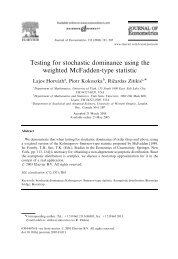
Linear <strong>Correlation</strong><br />
Linear <strong>Correlation</strong><br />
• Variables that are<br />
correlated through a<br />
linear relationship can<br />
display either positive<br />
or negative correlation<br />
• Positively correlated<br />
variables vary directly.<br />
Weight<br />
19<br />
18<br />
17<br />
16<br />
15<br />
14<br />
13<br />
12<br />
Regression Plot<br />
• Negatively correlated<br />
variables vary as<br />
opposites<br />
• As the value of one<br />
variable increases the<br />
other decreases<br />
Student GPA<br />
4<br />
3<br />
Regression Plot<br />
20<br />
21<br />
22<br />
Length<br />
23<br />
24<br />
2<br />
0<br />
10<br />
20<br />
Hours Worked<br />
30<br />
40<br />
Chapter 5 # 5<br />
Chapter 5 # 6<br />
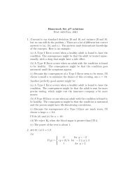
Strength of <strong>Correlation</strong><br />
Strength of <strong>Correlation</strong><br />
• <strong>Correlation</strong> may be strong,<br />
moderate, or weak.<br />
• You can estimate the<br />
strength be observing the<br />
variation of the points<br />
around the line<br />
• Large variation is weak<br />
correlation<br />
Student GPA<br />
4<br />
3<br />
Regression Plot<br />
• When the data is<br />
distributed quite close<br />
to the line the<br />
correlation is said to<br />
be strong<br />
• The correlation type is<br />
independent of the<br />
strength.<br />
Final Exam Score<br />
95<br />
90<br />
85<br />
80<br />
75<br />
70<br />
65<br />
60<br />
55<br />
50<br />
Regression Plot<br />
2<br />
55<br />
65<br />
75<br />
85<br />
95<br />
0<br />
10<br />
20<br />
Hours Worked<br />
30<br />
40<br />
Midterm Stats Grade<br />
Chapter 5 # 7<br />
Chapter 5 # 8
The <strong>Correlation</strong> Coefficient<br />
Interpreting r<br />
• The strength of a linear relationship is measured<br />
by the correlation coefficient<br />
• The sample correlation coefficient is given the<br />
symbol “r”<br />
• The population correlation coefficient has the<br />
symbol “ρ”.<br />
• The sign of the correlation coefficient tells us the<br />
direction of the linear relationship<br />
⎮ If r is negative ( 0) the correlation is positive. The<br />
line slopes up<br />
Chapter 5 # 9<br />
Chapter 5 # 10<br />
Interpreting r<br />
Cautions<br />
• The size (magnitude) of the correlation<br />
coefficient tells us the strength of a linear<br />
relationship<br />
⎮ If | r | > 0.90 implies a strong linear association<br />
⎮ For 0.65 < | r | < 0.90 implies a moderate linear<br />
association<br />
⎮ For | r | < 0.65 this is a weak linear association<br />
• The correlation coefficient only gives us an<br />
indication about the strength of a linear<br />
relationship.<br />
• Two variables may have a strong curvilinear<br />
relationship, but they could have a “weak” value<br />
for r<br />
Chapter 5 # 11<br />
Chapter 5 # 12
Fundamental Rule of <strong>Correlation</strong><br />
Setting<br />
• <strong>Correlation</strong> DOES NOT imply causation<br />
– Just because two variables are highly correlated does<br />
not mean that the explanatory variable “causes” the<br />
response<br />
• Recall the discussion about the correlation<br />
between sexual assaults and ice cream cone sales<br />
• A chemical engineer would like to determine if a<br />
relationship exists between the extrusion<br />
temperature and the strength of a certain<br />
formulation of plastic. She oversees the<br />
production of 15 batches of plastic at various<br />
temperatures and records the strength results.<br />
Chapter 5 # 13<br />
Chapter 5 # 14<br />
The Study Variables<br />
• The two variables of interest in this study are the strength<br />
of the plastic and the extrusion temperature.<br />
• The independent variable is extrusion temp. This is the<br />
variable over which the experimenter has control. She<br />
can set this at whatever level she sees as appropriate.<br />
• The response variable is strength. The value of “strength”<br />
is thought to be “dependent on” temperature.<br />
The Experimental Data<br />
Temp 120 125 130 135 140<br />
Str 18 22 28 31 36<br />
Temp 145 150 155 160 165<br />
Str 40 47 50 52 58<br />
Chapter 5 # 15<br />
Chapter 5 # 16
The <strong>Scatter</strong> Plot<br />
Conclusions by Inspection<br />
• The scatter diagram for<br />
the temperature versus<br />
strength data allows us to<br />
deduce the nature of the<br />
relationship between these<br />
two variables<br />
Strength (psi)<br />
60<br />
50<br />
40<br />
30<br />
20<br />
<strong>Scatter</strong> diagram of Strength vs Temperature<br />
120 130 140 150 160 170<br />
Temperature (F)<br />
• Does there appear to be a relationship between the<br />
study variables?<br />
• Classify the relationship as: Linear, curvilinear, no<br />
relationship<br />
• Classify the correlation as positive, negative, or no<br />
correlation<br />
• Classify the strength of the correlation as strong,<br />
moderate, weak, or none<br />
What can we conclude simply from the scatter diagram?<br />
Chapter 5 # 17<br />
Chapter 5 # 18<br />
Computing r<br />
Computing r<br />
r<br />
=<br />
1 ⎪⎧<br />
⎛<br />
Σ⎨<br />
⎜<br />
n −1<br />
⎪⎩ ⎝<br />
x − x ⎞⎛<br />
⎜<br />
y − y<br />
⎟<br />
s<br />
x ⎠⎝<br />
s y<br />
⎞⎪⎫<br />
⎟<br />
⎬<br />
⎠⎪⎭<br />
r<br />
=<br />
1<br />
Σ<br />
n −1<br />
[( )( )]<br />
Z x<br />
Z y<br />
df<br />
z-scores<br />
for x data<br />
z-scores<br />
for y data<br />
Chapter 5 # 19<br />
Chapter 5 # 20
Computing r - Example<br />
Classifying the strength of linear<br />
correlation<br />
See example handout for the plastic strength versus<br />
extrusion temperature setting<br />
•The strength of a linear correlation between the response<br />
and the explanatory variable can be assigned based on r<br />
These classifications are discipline dependent<br />
Chapter 5 # 21<br />
Chapter 5 # 22<br />
Classifying the strength of linear<br />
correlation<br />
For this class the following criteria are adopted:<br />
If |r| > 0.90 then the correlation is strong<br />
If |r| < 0.65 then the correlation is weak<br />
If 0.65 < |r| < 0.90 then the correlation is<br />
moderate<br />
<strong>Scatter</strong> <strong>Diagrams</strong> and Statistical<br />
Modeling and Regression<br />
• We’ve already seen that the best graphic for<br />
illustrating the relation between two quantitative<br />
variables is a scatter diagram. We’d like to take<br />
this concept a step farther and, actually develop a<br />
mathematical model for the relationship between<br />
two quantitative variables<br />
Chapter 5 # 23<br />
Chapter 5 # 24
The Line of Best Fit Plot<br />
Using the Line of Best Fit to Make<br />
Predictions<br />
• Since the data appears to<br />
be linearly related we can<br />
find a straight line model<br />
that fits the data better<br />
than all other possible<br />
straight line models.<br />
• This is the Line of Best<br />
Fit (LOBF)<br />
Strength<br />
60<br />
50<br />
40<br />
30<br />
20<br />
120<br />
130<br />
140<br />
Temp<br />
150<br />
160<br />
170<br />
• Based on this graphical<br />
model, what is the<br />
predicted strength for<br />
plastic that has been<br />
extruded at 142 degrees?<br />
Strength<br />
60<br />
50<br />
40<br />
30<br />
20<br />
120<br />
130<br />
140<br />
Temp<br />
150<br />
160<br />
170<br />
Chapter 5 # 25<br />
Chapter 5 # 26<br />
Using the Line of Best Fit to Make<br />
Predictions<br />
Using the Line of Best Fit to Make<br />
Predictions<br />
• Given a value for the<br />
predictor variable, determine<br />
the corresponding value of<br />
the dependent variable<br />
graphically.<br />
• Based on this model we<br />
would predict a strength of<br />
appx. 39 psi for plastic<br />
extruded at 142 F<br />
• Based on this graphical<br />
model, at what<br />
temperature would I need<br />
to extrude the plastic in<br />
order to achieve a strength<br />
of 45 psi?<br />
Strength<br />
60<br />
50<br />
40<br />
30<br />
20<br />
120<br />
130<br />
140<br />
Temp<br />
150<br />
160<br />
170<br />
Chapter 5 # 27<br />
Chapter 5 # 28
Using the Line of Best Fit to Make<br />
Predictions<br />
Computing the LSR model<br />
• Locate 45 on the response<br />
axis (y-axis)<br />
• Draw a horizontal line to<br />
the LOBF<br />
• Drop a vertical line down<br />
to the independent axis<br />
• The intercepted value is<br />
the temp. required to<br />
achieve a strength of 45<br />
psi<br />
• Given a LSR line for bivariate data, we can use that<br />
line to make predictions.<br />
• How do we come up with the best linear model<br />
from all possible models?<br />
Chapter 5 # 29<br />
Chapter 5 # 30<br />
Bivariate data and the sample linear<br />
regression model<br />
• For example, look at<br />
the fitted line plot of<br />
powerboat<br />
registrations and the<br />
number of manatees<br />
killed.<br />
• It appears that a linear<br />
model would be a<br />
good one.<br />
yˆ = b o + b1<br />
x<br />
Chapter 5 # 31<br />
The straight line model<br />
• Any straight line is completely defined by two<br />
parameters:<br />
⎮ The slope – steepness either positive or negative<br />
⎮ The y-intercept – this is where the graph crosses the<br />
vertical axis<br />
Chapter 5 # 32
The Parameter Estimators<br />
Calculating the Parameter Estimators<br />
• In our model “b 0 ” is the estimator for the<br />
intercept. The true value for this parameter is β 0<br />
• “b 1 ” estimates the slope. The true value for this<br />
• The equation for the LOBF is:<br />
yˆ = bo + b1<br />
x<br />
parameter is β 1<br />
Chapter 5 # 34<br />
Chapter 5 # 33<br />
Calculating the Parameter Estimators<br />
Computing the Intercept Estimator<br />
• To get the slope estimator we use:<br />
b<br />
b<br />
1<br />
or<br />
1<br />
=<br />
n Σ<br />
⎛<br />
= r<br />
⎜<br />
⎝<br />
n Σ<br />
s<br />
s<br />
( x y )<br />
y<br />
x<br />
2<br />
( x ) − ( Σ x )<br />
⎞<br />
⎟<br />
⎠<br />
−<br />
Σ<br />
x<br />
⋅<br />
Σ<br />
2<br />
y<br />
Chapter 5 # 35<br />
• The intercept estimator is computed from the<br />
variable means and the slope:<br />
b0 = y − b1<br />
x<br />
• Realize that both the slope and intercept<br />
estimated in these last two slides are really point<br />
estimates for the true slope and y-intercept<br />
Chapter 5 # 36
Revisit the manatee example<br />
Computing the estimators<br />
Look at the summary statistics and correlation<br />
coefficient data from the manatee example<br />
Variable N Mean SEMean StDev<br />
Boats 10 74.10 2.06 6.51<br />
Deaths 10 55.80 5.08 16.05<br />
Minitab correlation coefficient output<br />
<strong>Correlation</strong>s: Boats, Deaths<br />
Pearson correlation of Boats and Deaths = 0.921<br />
P-Value = 0.000<br />
So the slope is:<br />
b<br />
b<br />
1<br />
1<br />
⎛ s<br />
= r<br />
⎜<br />
⎝ s<br />
y<br />
x<br />
⎞<br />
⎟<br />
⎠<br />
⎛16.05<br />
⎞<br />
= 0.921⎜<br />
⎟ = 2.27<br />
⎝ 6.51 ⎠<br />
Chapter 5 # 37<br />
Chapter 5 # 38<br />
Computing the estimators<br />
Put it together<br />
And the intercept is calculated using the slope<br />
information along with the variable means:<br />
• In general terms any old linear regression<br />
equation is:<br />
response = intercept + slope(predictor)<br />
b<br />
0<br />
= y − b x<br />
1<br />
= 55.8 − 2.27<br />
= −112.4<br />
( 74.1)<br />
• Specifically for the manatee example the sample<br />
regression equation is:<br />
Deaths = -112.7 + 2.27(boats)<br />
Chapter 5 # 39<br />
Chapter 5 # 40
The slope estimate<br />
The slope estimate<br />
• b 1 is the estimated slope of the line<br />
• The interpretation of the slope is, “The amount of change<br />
in the response for every one unit change in the<br />
independent variable.”<br />
• In our example the estimated slope is 2.27<br />
• This is interpreted as, “For each additional 10,000 boats<br />
registered, an additional 2.27 more manatees are killed<br />
Chapter 5 # 41<br />
Chapter 5 # 42<br />
The intercept estimate<br />
The intercept Estimate<br />
• Recall the sample regression model:<br />
“b 0 ” is the estimated y- intercept<br />
yˆ = b0<br />
+ b1<br />
x<br />
The interpretation of the y-intercept is, “The<br />
value of the response when the control (or<br />
independent) variable has a value of 0.”<br />
• Sometimes this value is meaningful. For example<br />
resting metabolic rate versus ambient temperature in<br />
Centigrade ( o C)<br />
• Sometimes it’s not meaningful at all.<br />
• This is an example where the y-intercept just serves to<br />
make the model fit better. There can be no such thing as<br />
a –112.7 manatees killed<br />
Chapter 5 # 43<br />
Chapter 5 # 44
Regression Output<br />
Regression Output<br />
Use the minitab regression output for the<br />
manatee example to predict the expected<br />
number of manatees killed when the number of<br />
power boat registrations is 750,000 (x = 75)<br />
• The sample regression equation is:<br />
ManateesKilled = -112.7 + 2.27(boats)<br />
• So:<br />
ManateesKilled = -112.7 + 2.27(75) = 57.6<br />
• This means that we expect between 57 and 58<br />
manatees killed in a year where 750,000 power<br />
boats are registered.<br />
Chapter 5 # 45<br />
Chapter 5 # 46<br />
Regression Output<br />
Regression Output<br />
Use the minitab regression output for the<br />
manatee example to predict the expected<br />
number of manatees killed when the number of<br />
power boat registrations is 850,000 (x = 85)<br />
• The sample regression equation is:<br />
ManateesKilled = -112.7 + 2.27(boats)<br />
• So:<br />
ManateesKilled = -112.7 + 2.27(85) = 80.25<br />
• This means that we expect between 80 and 81<br />
manatees killed in a year where 750,000 power<br />
boats are registered.<br />
Chapter 5 # 47<br />
Chapter 5 # 48
Regression Output<br />
STOP!! YOU HAVE VIOLATED<br />
THE CARDINAL RULE OF REGRESSION<br />
Cardinal Rule of Regression<br />
• NEVER NEVER NEVER NEVER NEVER NEVER<br />
predict a response value from a predictor value that is<br />
outside of the experimental range.<br />
• The only predictions we can make (statistically) are<br />
predictions for responses where powerboat registrations<br />
are between 670,000 and 840,000.<br />
• This means that our prediction for the year when 850,000<br />
powerboats were registered is garbage<br />
Chapter 5 # 49<br />
Chapter 5 # 50<br />
Regression Estimates<br />
The coefficient of determination<br />
• r 2 is called the coefficient of determination.<br />
• r 2 is a proportion, so it is a number between 0 and 1<br />
inclusive.<br />
• r 2 quantifies the amount of variation in the response that is<br />
due to the variability in the predictor variable.<br />
• r 2 values close to 0 mean that our estimated model is a<br />
poor one while values close to 1 imply that our model<br />
does a great job explaining the variation<br />
The r 2 Value<br />
• If r 2 is, say, 0.857 we can conclude that 85.7% of the<br />
variability in the response is explained by the<br />
variability in the independent variable.<br />
• This leaves 100 - 85.7 = 14.3% left unexplained. It’s<br />
only the unexplained variation that is incorporated into<br />
the “uncertainty”<br />
Chapter 5 # 51<br />
Chapter 5 # 52
2 and the correlation coefficient<br />
<strong>Scatter</strong> of Points and r 2<br />
• r 2 is related to the correlation coefficient<br />
• It’s just the square of r<br />
• The interpretation as the proportion of variation in the<br />
response that is explained by the variation in the<br />
predictor variable makes it an important statistic<br />
r 2 = 0.848 r 2 = 0.992<br />
Chapter 5 # 53<br />
Chapter 5 # 54