Solution to Homework #12 - Statistics

Homework #12 solutions
Stat 530, Spring 2010
1. #8.15 We can use the Neymann-Pearson lemma because H 0 and H 1 are simple. Recall
from a previous problem (and the second exam) that T = ∑ n
i=1 X 2 i is sufficient for σ 2 ,
and we also know that T/σ 2 ∼ χ 2 (n), because the X i /σ are independent standard normal
random variables.
Therefore
and
g(t|σ 2 ) = 1 σ 2 1
Γ(n/1)2 n/2 ( t
σ 2 ) n/2−1
e −t/(2σ2 )
g(t|σ1)
2 ( ) σ
2 n/2−1 {
g(t|σ0) = 0
exp − 1 (
n∑ 1
x 2 2 σ1
2 i − 1 )}
.
2
i=1
σ1
2 σ0
2
A test that is UMP will reject H 0 if this ratio is “large” which is equivalent to rejecting
H 0 when ∑ n
i=1 x 2 i is “small,” as was to be shown. If α = 0.05, say, then we find c so that
or
P
( n
)
∑
P Xi 2 > c|σ0
2 = .05,
i=1
( n ∑
i=1
( ) 2 Xi
> c )
|σ 2
σ 0 σ0
2 0 = .05,
so we choose c = σ 2 0q, where q is the 95th percentile of a χ 2 (n) density.
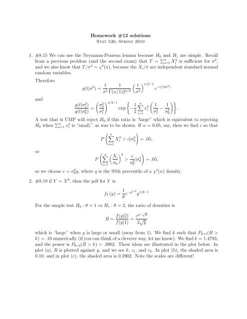
2. #8.19 if Y = X θ , then the pdf for Y is
f Y (y) = 1 θ e−y1/θ y 1/θ−1
For the simple test H 0 : θ = 1 vs H 1 : θ = 2, the ratio of densities is
R = f(y|2)
f(y|1) = ey−√ y
2 √ y
which is “large” when y is large or small (away from 1). We find k such that P θ=1 (R >
k) = .10 numerically (if you can think of a cleverer way, let me know). We find k = 1.4793,
and the power is P θ=2 (R > k) = .3902. These ideas are illustrated in the plot below. In
plot (a), R is plotted against y, and we see k, c 1 , and c 2 . In plot (b), the shaded area is
0.10, and in plot (c), the shaded area is 0.3902. Note the scales are different!

Another note: Clearly there are lots of different size-α tests for this problem. This test
does not have “equal probability tails” but we know that if we choose the size-α test that
does, it will have lower power.
(a)
(b)
(c)
R
1 2 3 4 5 6
k
c1
c2
0 1 2 3 4 5
exp(-yp)
0.0 0.2 0.4 0.6 0.8 1.0
c1
c2
0 1 2 3 4 5
exp(-sqrt(yp))/2/sqrt(yp)
0 1 2 3 4 5 6
c1
c2
0 1 2 3 4 5
Y
yp
yp
3. #8.20 The possible values of the ratio of the distributions are 6, 5, 4, 3, 2, 1, .79/.94, for x
values 1 through 7, respectively. We reject H 0 when the ratio is “large”, and if we want
α = .04, our decision rule is: reject H 0 when x ≤ 4. Then the power is P (X ≤ 4|H 1 ) = .18.
4. #8.22 Let Y = ∑ 10
i=1 X i , and note that Y is suffiecient for p. (a) We can compute
f(y|p = 1/4)
f(y|p = 1/2) = 3−y (3/2) 10 ,
so we reject when y is “small.” (We already did this for the likelihood ratio test, but
now we know it is UMP.) The probability that Y ≤ 2, under H 0 , is 0.0547. The power is
P (Y ≤ 2|H 1 ) = .526.
(b) P (Y ≥ 6) = .377 is the test size.
power
0.0 0.2 0.4 0.6 0.8 1.0
0.0 0.2 0.4 0.6 0.8 1.0
p

(c) The possible levels of α correspond to the possible decision rules. All decision rules
corresponding to UMP tests are of the form: reject H 0 when Y ≥ k, and for k = 1, . . . , 10,
the test sizes are 0.999, 0.989, 0.945, 0.828, 0.623, 0.377, 0.172, 0.055, 0.011, 0.001.
5. #8.25 (a) Choose any θ 1 < θ 2 . Then the likelihood ratio is
f(t|θ 2 )
f(t|θ 1 )
which is increasing in t.
{
= exp − 1 [
(t − θ2 ) 2 − (t − θ
2σ 2 1 ) 2]}
{
= exp − 1 [ ] } {
θ
2 1
2σ 2 2 − θ1
2 exp
σ t(θ 2 2 − θ 1 )}
(b) Choose any θ 1 < θ 2 . Then the likelihood ratio is
f(t|θ 2 )
f(t|θ 1 )
= e−θ2 θ2/t!
t
e −θ1 θ1/t!
t ( ) t
= e −(θ 2−θ 1 ) θ2
θ 1
which is increasing in t.
(c) Choose any θ 1 < θ 2 . Then the likelihood ratio is
f(t|θ 2 )
f(t|θ 1 )
=
(
n
t
(
n
t
)
)
θ t 2(1 − θ 2 ) n−t
θ t 1(1 − θ 1 ) n−t
=
( ) n ( ) t
1 − θ2 θ2 (1 − θ 1 )
1 − θ 1 θ 1 (1 − θ 2 )
which is increasing in t.
6. #8.31 We showed previously that the sum T = ∑ n
i=1 X i is sufficient for λ, and that T is
Poisson with mean nλ. Hence, by the previous problem, the family {g(t|λ) has MLR, so
that a UMP level-α test is of the form: reject H 0 iff T > t 0 . For example, if n = 20 and
if we want α ≈ .01, we reject H 0 if T > 79, and α = .00782.
7. #8.34 (a) If g(t|θ) = h(t − θ), then
P θ1 (T > c) =
∫ ∞
c
g(tθ 1 )dt

=
=
∫ ∞
c
∫ ∞
h(t − θ 1 )dt
c−θ 1
h(u)du
∫ ∞
≥ h(u)du
c−θ 2
≥ P θ2 (T > c)
where the first inequality is because θ 2 > θ 1 and h(u) ≥ 0.
(b) Suppose the family has increasing MLR, and consider θ 1 > θ 0 . By the the Neymann-
Pearson lemma, the test that rejects H 0 if g(t|θ 1 )/g(t|θ 0 ) > k is a UMP level-α test where
α = P θ0 (g(t|θ 1 )/g(t|θ 0 ) > k). Because the ratio g(t|θ 1 )/g(t|θ 0 ) is monotone increasing
in t, this test is equivalent to: reject H 0 if T > t 0 , where α = P θ0 (T > t 0 ). Then the
corollary to the Neymann-Pearson lemma says that the power is larger than the test size,
so P θ1 (T > t 0 ) > P θ0 (T > t 0 ) which was what we wanted.
8. #8.37 (a) Consider the sufficient statistic T = ¯X. Using T , we get that the likelihood
ratio is
λ(t) = sup 1
θ≤θ 0
e − 1
2πσ 2 2σ 2 (t−θ)2
1
sup θ e − 1
2πσ 2 2σ 2 (t−θ)2
We know that the MLE for θ is t, so if t = ¯x ≤ θ 0 , λ(t) = 1 and we accept H 0 . If ¯x > t,
then the maximum of the numerator occurs at θ 0 , and we get: reject H 0 if
e − 1
2σ 2 (t−θ 0) 2
is large, which occurs when t−θ 0 is large. Therefore, we get the same test in the likelihood
ratio approach.
(b) We showed in a previous problem that the family g(¯x|θ) has increasing MLR, so we
reject H 0 when T > t 0 for the UMP level-α test.
(c) For unknown σ 2 , we write the likelihood ratio as
λ(x) =
) n
2
exp{− 1 ∑ ni=1
(x
2πˆσ 0
2 2ˆσ 0
2 i − ˆθ 0 ) 2 }
( ) n
1 2
exp{− 1 ∑ ni=1
(x
2πˆσ 2 2ˆσ 2 i − ˆθ)
.
2 }
( 1
when ¯x ≤ θ 0 , the ratio is 1, but when ¯x > θ 0 , we have ˆθ 0 = θ 0 and
ˆσ 0 2 = 1 n∑
(x i − θ 0 ) 2 ,
n
i=1

while ˆθ = ¯x and ˆσ 2 = ∑ n
i=1 (x i − ¯x) 2 . Then
λ(x) =
[ ∑ ni=1
(x i − ¯x) 2 ] n
2
∑ ni=1 .
(x i − θ 0 ) 2
The null hypothesis is rejected when this is small, or when
∑ ni=1
(x i − θ 0 ) 2
∑ ni=1
(x i − ¯x) 2
is large. This can be written as
∑ ni=1
(x i − ¯x) 2 + n(¯x − θ 0 ) 2
∑ ni=1
(x i − ¯x) 2 = 1 + n(¯x − θ 0) 2
so we can reject H 0 when
(¯x − θ 0 ) 2
is large. This is when
¯x − θ 0
S
is large or small, which leads to the t-test.
9. #8.41 (a) The likelihood is
L(µ X , µ Y , σ 2 |x, y) =
S 2
(n − 1)S 2
( ) 1 (n+m)/2
{
exp − 1 [
∑ n
(x
2πσ 2 2σ 2 i − µ x ) 2 +
i=1
]}
m∑
(y i − µ y ) 2
i=1
Taking the log, partial derivatives with respect to the three parameters, and setting to
zero, etc., gives the usual MLEs:
ˆµ x = 1 n∑
x i = ¯x,
n
i=1
ˆµ y = 1 m∑
y i = ȳ,
m
i=1
and
ˆσ 2 = 1 [ n
]
∑
m∑
(x i − ¯x) 2 + (y i − ȳ) 2 .
m + n
i=1
i=1
Restricting µ x = µ y = µ, the MLE for µ is
ˆµ 0 =
∑ ni=1
x i + ∑ m
i=1 y i
m + n

and for σ 2 we get
Then the likelihood ratio is
[ ] m+n {
ˆσ
2 2
λ(x, y) = exp
=
ˆσ 2 0
[ ˆσ
2
ˆσ 2 0
] m+n
2
.
ˆσ 0 2 = 1 [
∑ n
(x i − ˆµ 0 ) 2 +
m + n
i=1
− 1
2ˆσ 2 0
[ n ∑
(x i − ˆµ 0 ) 2 +
i=1
]
n∑
(y i − ˆµ 0 ) 2
i=1
]
m∑
(y i − ˆµ 0 ) 2 + 1 [ n
]}
∑
m∑
(x
i=1
2ˆσ 2 i − ¯x) 2 − (y i − ȳ) 2
i=1
i=1
Now,
(m + n)ˆσ 0 2 =
n∑ m∑
x 2 i + yi 2 − 2(n¯x + mȳ)ˆµ 0 + (m + n)ˆµ 2 0
i=1 i=1
=
n∑
n∑
(x i − ¯x) 2 + n¯x 2 + (y i − ȳ) 2 + mȳ 2 − 2(n¯x + mȳ)ˆµ 0 + (m + n)ˆµ 2 0
i=1
i=1
= (m + n)ˆσ 2 + n¯x 2 + mȳ 2 (mȳ + n¯x)2
−
m + n
= (m + n)ˆσ 2 + mn
m + n (¯x − ȳ)2 .
So,
ˆσ 0
2
ˆσ = 1 + mn ( ) ¯x − ȳ 2
.
2 (m + n) 2 ˆσ
Then λ(x, y) is small when |¯x − ȳ|/ˆσ is large, and ˆσ 2 is proportional to Sp.
2
(b) Because under H 0 , the X i and Y i values are iid, we have shown that Sp 2 is an unbiased
estimator of σ 2 and (m + n − 2)Sp/σ 2 2 ∼ χ 2 (n + m − 2). We also know that (¯x − ȳ) is
normal with mean zero and variance (1/m + 1/n)σ 2 . Therefore,
¯x − ȳ
Z =
∼ N(0, 1).
√(1/m + 1/n)σ2 We also showed that ¯X and ∑ n
i=1 (X i − ¯X) 2 are independent and ditto for the Y -values,
so that Z and S 2 p are independent. Then
T =
Z
√
(m + n − 2)S
2
p /σ 2 /(m + n − 2)
∼ t(m + n − 2).
(c) If the “core” measurements are the x i and the “periphery” measurements are the y i ,
then I get ¯x = 1249.857 and ȳ = 1261.333 and S 2 p = 433.13, so the observed value of the
T statistic is t = −1.291, and te p-value is .21. We accept H 0 and conclude there the
means are the same.