MetaMorphs - Webdocs Cs Ualberta
MetaMorphs - Webdocs Cs Ualberta
MetaMorphs - Webdocs Cs Ualberta

You also want an ePaper? Increase the reach of your titles
YUMPU automatically turns print PDFs into web optimized ePapers that Google loves.
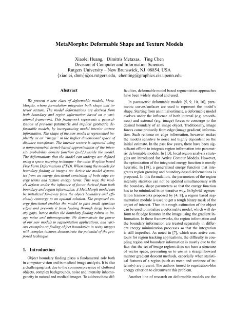
<strong>MetaMorphs</strong>: Deformable Shape and Texture Models<br />
Xiaolei Huang, Dimitris Metaxas, Ting Chen<br />
Division of Computer and Information Sciences<br />
Rutgers University – New Brunswick, NJ 08854, USA<br />
{xiaolei, dnm}@cs.rutgers.edu, chenting@graphics.cis.upenn.edu<br />
Abstract<br />
We present a new class of deformable models, Meta-<br />
Morphs, whose formulation integrates both shape and interior<br />
texture. The model deformations are derived from<br />
both boundary and region information based on a variational<br />
framework. This framework represents a generalization<br />
of previous parametric and implicit geometric deformable<br />
models, by incorporating model interior texture<br />
information. The shape of the new model is represented implicitly<br />
as an “image” in the higher dimensional space of<br />
distance transforms. The interior texture is captured using<br />
a nonparametric kernel-based approximation of the intensity<br />
probability density function (p.d.f.) inside the model.<br />
The deformations that the model can undergo are defined<br />
using a space warping technique - the cubic B-spline based<br />
Free Form Deformations (FFD). When using the models for<br />
boundary finding in images, we derive the model dynamics<br />
from an energy functional consisting of both edge energy<br />
terms and texture energy terms. This way, the models<br />
deform under the influence of forces derived from both<br />
boundary and region information. A MetaMorph model can<br />
be initialized far-away from the object boundary and efficiently<br />
converge to an optimal solution. The proposed energy<br />
functional enables the model to pass small spurious<br />
edges and prevents it from leaking through large boundary<br />
gaps, hence makes the boundary finding robust to image<br />
noise and inhomogeneity. We demonstrate the power<br />
of our new models to segmentation applications, and various<br />
examples on finding object boundaries in noisy images<br />
with complex textures demonstrate the potential of the proposed<br />
technique.<br />
1. Introduction<br />
Object boundary finding plays a fundamental role both<br />
in computer vision and in medical image analysis. It is also<br />
a challenging task due to the common presence of cluttered<br />
objects, complex backgrounds, noise and intensity inhomogeneity<br />
in natural and medical images. To address these difficulties,<br />
deformable model based segmentation approaches<br />
have been widely studied and used.<br />
In parametric deformable models [5, 9, 10, 16], parametric<br />
curves/surfaces are used to represent the model’s<br />
shape. Starting from an initial estimate, a deformable model<br />
evolves under the influence of both internal (e.g. smoothness)<br />
and external (e.g. image) forces to converge to the<br />
desired boundary of an image object. Traditionally, image<br />
forces come primarily from edge (image gradient) information.<br />
Such reliance on edge information, however, makes<br />
the models sensitive to noise and highly dependent on the<br />
initial estimate. In the past few years, there have been significant<br />
efforts to integrate region information into parametric<br />
deformable models. In [13], local region analysis strategies<br />
are introduced for Active Contour Models. However,<br />
the optimization of the integrated energy function is mostly<br />
heuristic. In [18], a generalized energy function that integrates<br />
region growing and boundary-based deformations is<br />
proposed. In this formulation, the parameters of the region<br />
intensity statistics can not be updated simultaneously with<br />
the boundary shape parameters so that the energy function<br />
has to be minimized in an iterative way. In hybrid segmentation<br />
frameworks proposed by [4, 8], a region based segmentation<br />
module is used to get a rough binary mask of the<br />
object of interest. Then this rough estimation of the object<br />
can be used to initialize a deformable model, which will deform<br />
to fit edge features in the image using the gradient information.<br />
In these frameworks, the region information and<br />
the boundary information are treated separately in different<br />
energy minimization processes so that the integration<br />
is still imperfect. As noted in [7], which uses active contours<br />
for region tracking applications, the difficulty in coupling<br />
region and boundary information is mostly due to the<br />
fact that the set of image regions does not have a structure<br />
of vector space, preventing us to use in a straightforward<br />
manner gradient descent methods, especially when statistical<br />
features of a region (such as mean and variance of intensity)<br />
are present. The authors turned to registration-like<br />
energy criterion to circumvent this problem.<br />
Another line of research on deformable models are the
implicit geometric models [3, 11, 12, 14, 17], which are<br />
implemented in the level set based curve evolution framework.<br />
In the Mumford and Shah model for segmentation<br />
[11], an optimal piecewise smooth function is pursued to approximate<br />
an observed image, such that the function varies<br />
smoothly within each region, and rapidly or discontinuously<br />
across the boundaries of different regions. Solutions for the<br />
reduced cases of this minimal partition problem have been<br />
proposed in the level set framework [17]. In [12, 14], variational<br />
frameworks are proposed for image segmentation by<br />
unifying boundary and region-based information sources,<br />
and level set approaches are used to implement the resulting<br />
PDE systems. However, all these frameworks assume piecewise<br />
constant, or Gaussian intensity distributions within<br />
each partitioned region. This limits their power and robustness<br />
in finding objects whose interiors have high noise level,<br />
intensity inhomogeneity, and/or complex multi-modal intensity<br />
distributions. Furthermore, the computational cost of<br />
these level-set based implementations tends to be high.<br />
To address the above limitations in previous efforts to<br />
incorporate region information in deformable models, we<br />
introduce in this paper a new class of deformable models,<br />
which we term “<strong>MetaMorphs</strong>”. The MetaMorph models<br />
possess both shape and interior texture, and integrate<br />
boundary and region information coherently in a common<br />
variational framework. The model shapes in our framework<br />
are embedded in a higher dimensional space of distance<br />
transforms, thus represented by distance map “images”.<br />
The model deformations are efficiently parameterized<br />
using the cubic B-spline based Free Form Deformations<br />
(FFD) [1, 2, 6]. The interior intensity statistics of the<br />
models are captured using nonparametric kernel-based approximations,<br />
which can represent complex multi-modal<br />
distributions. When finding object boundaries in images,<br />
the dynamics of the MetaMorph models are derived from<br />
an energy functional consisting of both edge/boundary energy<br />
terms and intensity/region energy terms. In our formulation,<br />
both types of energy terms are differentiable with respect<br />
to the model deformation parameters. This allows for<br />
a unified gradient-descent based deformation parameter updating<br />
paradigm using both boundary and region information.<br />
During model evolution, the boundary and region energy<br />
terms will have complementary effects. They will aid<br />
the model to grow/shrink and overcome local minima due to<br />
small spurious edges inside the object, to prevent the model<br />
from leaking at boundary gaps, and to enable the segmentation<br />
of objects with intensity inhomogeneity and complex<br />
interior statistics.<br />
The remainder of the paper is organized as follows. In<br />
section 2, we introduce the shape and texture representations<br />
of the MetaMorph models. In section 3, we derive the<br />
MetaMorph model dynamics from both boundary and region<br />
information. In section 4, the overall model fitting al-<br />
(1)<br />
(2)<br />
(a) (b) (c)<br />
Figure 1. Shape representation and deformations of the<br />
MetaMorph models. (1) The model shape. (2) The implicit<br />
“image” representation of the model shape. (a) Initial<br />
model. (b) Example FFD control lattice deformation to<br />
expand the model. (c) Another example of the free-form<br />
model deformation given the control lattice deformation.<br />
gorithm and experimental results are presented, and we conclude<br />
with discussions in section 5.<br />
2. The MetaMorph Models<br />
In this section, we present the shape and texture representations<br />
of the MetaMorph deformable models, and define<br />
the model deformations.<br />
2.1. The Model’s Shape Representation<br />
The model’s shape is embedded implicitly in a higher dimensional<br />
space of distance transforms. The Euclidean distance<br />
transform is used to embed an evolving model as the<br />
zero level set of a higher dimensional distance function. In<br />
order to facilitate notation, we consider the 2D case. Let<br />
Φ : Ω → R + be a Lipschitz function that refers to the distance<br />
transform for the model shape M. By definition Ω is<br />
bounded since it refers to the image domain. The shape defines<br />
a partition of the domain: the region that is enclosed by<br />
M, [R M ], the background [Ω − R M ], and on the model,<br />
[∂R M ] (In practice, we consider a narrow band around the<br />
model M in the image domain as ∂R M ). Given these definitions<br />
the following implicit shape representation is considered:<br />
⎧<br />
⎨<br />
0, x ∈ ∂R M<br />
Φ M (x) = +ED(x, M) > 0, x ∈ R M<br />
⎩<br />
−ED(x, M) < 0, x ∈ [Ω − R M ]<br />
where ED(x, M) refers to the min Euclidean distance between<br />
the image pixel location x = (x, y) and the model<br />
M.<br />
Such treatment makes the model shape representation an<br />
“image”, which greatly facilitates the integration of boundary<br />
and region information. It also provides a feature space
0.3<br />
0.25<br />
0.2<br />
0.15<br />
0.1<br />
0.05<br />
0.3<br />
0.25<br />
0.2<br />
0.15<br />
0.1<br />
0.05<br />
0.3<br />
0.25<br />
0.2<br />
0.15<br />
0.1<br />
0.05<br />
0<br />
50 100 150 200 250<br />
0<br />
50 100 150 200 250<br />
0<br />
50 100 150 200 250<br />
in which objective functions that are optimized using a gradient<br />
descent method can be conveniently used. A sufficient<br />
condition for convergence of the gradient descent methods<br />
requires continuous first derivatives. The considered<br />
implicit representation satisfies such a condition. One can<br />
prove that the gradient of the distance function is a unit vector<br />
in the normal direction of the shape. This property will<br />
make our model evolution fast. Examples of this implicit<br />
representation can be found in [Fig. (1).2]. This shape representation<br />
in 3D is similarly defined in a volumetric embedding<br />
space.<br />
(1)<br />
0<br />
(2)<br />
0<br />
2.2. The Model’s Deformations<br />
The deformations that MetaMorph models can undergo<br />
are defined using a space warping technique, the Free Form<br />
Deformations (FFD) [15]. The essence of FFD is to deform<br />
an object by manipulating a regular control lattice F overlaid<br />
on its volumetric embedding space. One of the main<br />
advantages of the FFD technique is that it imposes implicit<br />
smoothness constraints during deformation, since it guarantees<br />
C 1 continuity at control points and C 2 continuity<br />
everywhere else. Therefore there is no need for introducing<br />
computationally expensive regularization components<br />
on the deformed shapes. Another advantage is that, since<br />
FFD is a space warping technique, it integrates naturally<br />
with the implicit model shape representation in a higher dimensional<br />
embedding space. In this paper, we consider an<br />
Incremental Free Form Deformations (IFFD) formulation<br />
using the cubic B-spline basis [6].<br />
Let us consider a regular lattice of control points<br />
F m,n = (F x m,n, F y m,n); m = 1, ..., M,<br />
n = 1, ..., N<br />
overlaid to a region Γ c = {x} = {(x, y)|1 ≤ x ≤ X, 1 ≤<br />
y ≤ Y } in the embedding space that encloses the model in<br />
its object-centered coordinate system. Let us denote the initial<br />
configuration of the control lattice as F 0 , and the deforming<br />
control lattice as F = F 0 + δF . Under these assumptions,<br />
the incremental FFD parameters, which are also<br />
the deformation parameters for the model, are the deformations<br />
of the control points in both directions (x, y):<br />
q = {(δF x m,n, δF y m,n)}; (m, n) ∈ [1, M] × [1, N]<br />
The deformed position of a pixel x = (x, y) given the deformation<br />
of the control lattice from F 0 to F , is defined in<br />
terms of a tensor product of Cubic B-spline polynomials:<br />
D(q; x) = x + δD(q; x) =<br />
3∑<br />
k=0 l=0<br />
3∑<br />
B k (u)B l (v)<br />
(F 0 i+k,j+l + δF i+k,j+l ) (1)<br />
where i = ⌊ x X · (M − 1)⌋ + 1, j = ⌊ y Y · (N − 1)⌋ + 1. The<br />
terms of the deformation component refer to:<br />
(3)<br />
0<br />
(a) (b) (c) (d)<br />
Figure 2. The Endocardium segmentation. (1) Initial<br />
model. (2) Intermediate result. (3) Final converged result.<br />
(a) The evolving model drawn in colored lines (blue or red)<br />
on original image. (b) Interior of the evolving model. (c)<br />
The intensity p.d.f of the model interior. The X axis is the<br />
intensity value in the range of [0, 255] and the Y axis is the<br />
probability value in the range of [0, 1]. (d) The image probability<br />
map based on the p.d.f of the model interior.<br />
• δF i+l,j+l , (k, l) ∈ [0, 3] × [0, 3] are the deformations<br />
of pixel x’s (sixteen) adjacent control points,<br />
• B k (u) is the k th basis function of a Cubic B-spine, defined<br />
by:<br />
B 0 (u) = (1 − u) 3 /6, B 1 (u) = (3u 3 − 6u 2 + 4)/6<br />
B 2 (u) = (−3u 3 + 3u 2 + 3u + 1)/6, B 3 (u) = u 3 /6<br />
with u = x X · (M − 1) − ⌊ x X · (M − 1)⌋. B l(v) is<br />
similarly defined.<br />
• δD(q; x) = ∑ 3<br />
k=0<br />
∑ 3<br />
l=0 B k(u)B l (v)δF i+k,j+l is the<br />
incremental deformation for pixel x.<br />
One example for the model deformations is shown in<br />
[Fig. (1)]. An initial model is shown in [Fig. (1).a], with regular<br />
control lattice. When its embedding space deforms due<br />
to the deformation of the FFD control lattice as shown in<br />
[Fig. (1).b], the model undergoes an expansion in its objectcentered<br />
coordinate system. [Fig. (1).c] shows another example<br />
of free-form model deformation given the FFD control<br />
lattice deformation.<br />
The extension of the models to account for deformations<br />
in 3D is straightforward, by using control lattices in the 3D<br />
space and a 3D tensor product of B-spline polynomials.<br />
2.3. The Model’s Texture<br />
Rather than using traditional statistical parameters (such<br />
as mean and variance) to approximate the intensity distribution<br />
of the model interior, we model the distribution using
a nonparametric kernel-based method. The nonparametric<br />
approximation is differentiable, more generic and can represent<br />
complex multi-modal intensity distributions.<br />
Suppose the model is placed on an image I, the image region<br />
bounded by current model Φ M is R M , then the probability<br />
of a pixel’s intensity value i being consistent with<br />
the model interior intensity can be derived using a Gaussian<br />
kernel as:<br />
P(i ∣ ∫∫<br />
1<br />
1<br />
∣Φ M ) =<br />
√ e −(i−I(y))2<br />
2σ<br />
V (R M )<br />
2 dy (2)<br />
R M 2πσ<br />
where V (R M ) denotes the volume of R M , and σ is a constant<br />
specifying the width of the gaussian kernel.<br />
Using this nonparametric approximation, the intensity<br />
distribution of the model interior gets updated automatically<br />
while the model deforms. The initialization of the model<br />
texture is flexible. We can either start with a small model inside<br />
the texture region to be segmented, or use supervised<br />
learning to specify the desired texture a Priori. One example<br />
of the model interior texture representation can be seen in<br />
[Fig. (2)]. In the figure, we show the zero level set of the current<br />
model Φ M in colored lines [Fig. (2).a], the model interior<br />
region R M [Fig. (2).b], the probability density function<br />
(p.d.f.) for the intensity of current model interior P(i ∣ ∣Φ M )<br />
for i = 0, ...255 [Fig. (2).c], and the probability map of every<br />
pixel’s intensity in the image according to the model interior<br />
distribution [Fig. (2).d].<br />
3. The MetaMorph Dynamics<br />
We demonstrate the MetaMorph model fitting dynamics<br />
in the context object segmentation. However, the approach<br />
is general and can be applied to many other computer vision<br />
problems<br />
In order to fit to the boundary of an object, the motion<br />
of the model is driven by both gradient (edge) energy terms<br />
and texture (intensity) energy terms derived from the image.<br />
The overall energy functional E consists of two parts –<br />
the shape data terms E S , and the intensity data terms E I :<br />
E = E S + kE I (3)<br />
where k is a constant balancing the contribution of the two<br />
parts. In our formulation, we are able to omit the model<br />
smoothness term in traditional parametric or level-set based<br />
deformable models, since this smoothness is implicit by using<br />
the Free Form Deformations. Next, we derive the shape<br />
and intensity data terms respectively.<br />
3.1. The Shape Data Terms<br />
The gradient information is a very important source of<br />
the image forces for a deformable model. We encode the<br />
gradient information of an image using a “shape image” Φ,<br />
which is derived from the un-signed distance transform of<br />
(a) (b) (c)<br />
Figure 4. The effect of small spurious edges inside the<br />
object of interest (endocardium of the Left Ventricle) on the<br />
“shape image”. (a) The original MR image. (b) The edge<br />
map of the image. (c) The derived “shape image”, with<br />
edges points drawn in yellow. Note the effect of the small<br />
spurious edges on the “shape image” inside the object.<br />
the edge map of the image. In [Fig. (4).c], we can see the<br />
“shape image” of an example MR heart image.<br />
To evolve a MetaMorph model toward image edges, we<br />
define two shape data terms – an interior term E Si and a<br />
boundary term E Sb :<br />
E S = E Si + aE Sb (4)<br />
3.1.1. The Interior Shape Data Term In the interior<br />
shape data term of the model, we aim to minimize the<br />
Sum-of-Squared-Differences between the implicit shape<br />
representation values in the model interior and the underlying<br />
“shape image” values at corresponding deformed<br />
positions. This can be written as:<br />
E Si =<br />
1<br />
V (R M )<br />
∫∫<br />
R M<br />
(<br />
ΦM (x) − Φ(D(q; x)) ) 2<br />
dx (5)<br />
During optimization, this term will deform the model along<br />
the gradient direction of the underlying “shape image”.<br />
Thus it will expand or shrink the model accordingly, serving<br />
as a two-way balloon force without explicitly introducing<br />
such forces, and making the attraction range of the model<br />
large.<br />
3.1.2. The Boundary Shape Data Term The previous<br />
interior shape term is good in attracting the model toward<br />
boundary structures from far-away locations. However,<br />
when there are small spurious edges detected within<br />
an object due to texture, the “shape image” inside the object<br />
could differ in the surrounding areas of those small edges.<br />
One such example can be seen in [Fig. (4).a-c]. To make<br />
the model deformation more robust to such situations, we<br />
consider a separated boundary shape data term, which allows<br />
higher weights for pixels in a narrow band around the<br />
model boundary ∂R M .<br />
E Sb =<br />
1<br />
V (∂R M )<br />
∫∫<br />
∂R M<br />
(<br />
Φ(D(q; x))<br />
) 2dx (6)<br />
Intuitively, this term will encourage the deformation that<br />
maps the model boundary to the image edge locations where
7 8 8 8 8 8 9 9 8 8 7 7 6 6 5 5 4 4 3 2 1 1 0 1 2 3 2 1 0 1 2<br />
8 8 9 9 9 9 9 109 9 8 8 7 7 6 6 5 4 4 3 2 1 0 1 2 3 2 1 0 1 1<br />
9 9 101010101011109 9 9 8 8 7 6 5 4 4 3 2 1 0 1 2 3 2 1 1 0 1<br />
9 101111111111111110109 8 7 6 5 4 4 3 2 1 1 0 1 2 3 3 2 1 0 1<br />
101111121212121111109 9 8 7 6 5 4 3 2 1 1 0 1 1 2 3 3 2 1 0 1<br />
1112121313121111109 9 8 8 7 6 5 4 3 2 1 0 1 1 2 3 4 3 2 1 0 1<br />
12131313121111109 8 8 7 7 6 6 5 4 3 2 1 0 1 2 3 4 4 3 2 1 0 1<br />
131313121111109 8 8 7 6 6 5 5 5 4 3 2 1 0 1 1 2 3 4 3 2 1 0 1<br />
1413131211109 8 8 7 6 6 5 4 4 4 4 3 2 1 1 0 1 2 3 4 3 2 1 0 1<br />
14131211109 9 8 7 6 6 5 4 4 3 3 3 3 3 2 1 0 1 2 3 4 3 2 1 0 1<br />
14131211109 8 7 6 6 5 4 4 3 2 2 2 2 3 2 1 0 1 2 3 4 3 2 1 1 0<br />
131211109 9 8 7 6 5 4 4 3 2 1 1 1 1 2 2 1 1 1 2 3 4 4 3 2 1 0<br />
131211109 8 7 6 5 4 4 3 2 1 1 0 0 1 2 3 2 2 2 3 4 4 4 3 2 1 0<br />
131211109 8 7 6 5 4 3 2 1 1 0 1 1 1 2 3 3 3 3 4 4 4 4 3 2 1 0<br />
131211109 8 7 6 5 4 3 2 1 0 1 1 2 2 3 4 4 4 4 4 5 4 3 2 1 1 0<br />
121111109 8 7 6 5 4 3 2 1 0 1 2 3 3 4 4 5 5 5 5 5 4 3 2 1 0 1<br />
1211109 8 8 7 6 5 4 3 2 1 0 1 2 3 4 4 5 6 6 6 6 5 4 3 2 1 0 1<br />
11109 9 8 7 6 5 4 4 3 2 1 0 1 2 3 4 5 6 6 7 7 6 5 4 3 2 1 0 1<br />
11109 8 7 6 6 5 4 3 2 1 1 0 1 2 3 4 5 6 7 7 6 5 4 4 3 2 1 0 1<br />
109 8 8 7 6 5 4 4 3 2 1 0 1 1 2 3 4 5 6 7 7 6 5 4 3 2 1 1 0 1<br />
9 8 8 7 6 5 4 4 3 2 1 1 0 1 2 3 4 4 5 6 7 6 5 4 4 3 2 1 0 1 1<br />
8 8 7 6 6 5 4 3 2 1 1 0 1 1 2 3 4 5 6 7 6 6 5 4 3 2 1 1 0 1 2<br />
7 7 6 6 5 4 4 3 2 1 0 1 1 2 3 4 4 5 6 7 6 5 4 4 3 2 1 0 1 1 2<br />
6 6 5 5 4 4 3 2 1 1 0 1 2 3 4 4 5 6 7 6 5 4 4 3 2 1 1 0 1 2 3<br />
5 5 4 4 4 3 2 1 1 0 1 1 2 3 4 5 6 6 6 6 5 4 3 2 1 1 0 1 1 2 3<br />
4 4 4 3 3 2 1 1 0 1 1 2 3 4 4 5 6 6 6 5 4 4 3 2 1 0 1 1 2 3 4<br />
3 4 3 2 2 1 1 0 1 1 2 3 4 4 5 6 6 6 5 4 4 3 2 1 1 0 1 2 3 4 4<br />
2 3 2 1 1 1 0 1 1 2 3 4 4 5 6 6 6 5 4 4 3 2 1 1 0 1 1 2 3 4 5<br />
1 2 1 1 0 0 1 1 2 3 4 4 5 6 6 5 5 4 4 3 2 1 1 0 1 1 2 3 4 4 5<br />
1 2 1 0 1 1 1 2 3 4 4 5 6 6 5 4 4 4 3 2 1 1 0 1 1 2 3 4 4 4 4<br />
1 1 1 0 1 2 2 3 4 4 5 6 5 5 4 4 3 3 2 1 1 0 1 1 2 3 4 3 3 3 3<br />
(a) (b) (c) (d)<br />
Figure 3. The boundary shape data term constraints at small gaps in the edge map. (a) Original Image. (b) The edge map, note the<br />
small gap inside the red square region. (c) The “shape image”. (d) Zoom-in view of the region inside the red square. The numbers<br />
are the “shape image” values at each pixel location. The red dots are edge points, the blue squares indicate a path favored by the<br />
boundary term for a MetaMorph model.<br />
the underlying “shape image” distance values are as small<br />
(or as close to zero) as possible. In the shape energy functional<br />
[Eqn. (4)], by setting the value of constant a > 1,<br />
those model boundary pixels get higher weights.<br />
One additional advantage of the boundary shape data<br />
term is that, at an edge with small gaps, this term will constrain<br />
the model to go along the “geodesic” path, which coincides<br />
with the smooth shortest path connecting the two<br />
open ends of a gap. This behavior can be seen from [Fig.<br />
(3)]. Note that at a small gap of the edge map, the boundary<br />
term will favor a path with the smallest accumulative<br />
distance values to the edge points.<br />
3.2. The Intensity Data Terms<br />
One of the most attractive aspects of our MetaMorph deformable<br />
models is that they possess interior texture, and<br />
their deformations are influenced by forces derived from<br />
image region information. This information is very important<br />
to help the models out of local minima, and converge to<br />
the true object boundaries. In [Fig. (4)], the spurious edges<br />
both inside and around the object boundary degrade the reliability<br />
of the “shape image” and the shape data terms. Yet<br />
the intensity probability map computed based on the interior<br />
texture of an initial model, as shown in [Fig. (2).1.d],<br />
gives a pretty clear indication of the rough boundary of the<br />
object. In another MR heart image shown in [Fig. (6).1.a], a<br />
large portion of the object (Endocardium) boundary is missing<br />
during computation of the edge map, due to errors in<br />
edge detection [Fig. (6).1.b]. Relying solely on the “shape<br />
image” [Fig. (6).1.c] and shape data terms, a model would<br />
have leaked through the large gap and mistakenly converged<br />
to the outer epicardium boundary. In this situation, the intensity<br />
probability maps [Fig. (6).2-4.d] computed based<br />
on the model interior statistics become the key to optimal<br />
model convergence.<br />
(a) (b) (c) (d)<br />
Figure 5. Deriving the “region of interest” intensity data<br />
term. (a) The model shown (in yellow) on the original image.<br />
(b) The intensity probability map based on the model<br />
interior statistics. (c) The region of interest (ROI) derived<br />
from the thresholded probability map. The threshold is the<br />
mean probability over the entire image. (d) The “shape image”<br />
encoding boundary information of the ROI.<br />
In our framework, the intensity energy function E I consists<br />
of two intensity data terms – a “Region Of Interest”<br />
(ROI) term E Ir , and a Maximum Likelihood term E Im :<br />
E I = E Ir + bE Im (7)<br />
3.2.1. The ROI Intensity Data Term In the “Region Of<br />
Interest” (ROI) term, we aim to evolve the model toward the<br />
boundary of current region of interest, which is determined<br />
based on current model interior intensity distribution.<br />
Given a model M on image I [Fig. (5).a], we first compute<br />
the image intensity probability map P I [Fig. (5).b],<br />
based on the model interior intensity statistics (see section<br />
2.3). Then a small threshold (typically the mean probability<br />
over the entire image domain) is applied on P I to produce<br />
a binary image BP I , in which pixels with probabilities<br />
higher than the threshold have value 1. Morphological<br />
operations are used to fill in small holes in BP I . We then<br />
take the connected component on this binary image overlapping<br />
the model as current region of interest (ROI). Suppose<br />
the binary mask of this ROI is BI r [Fig. (5).c], we en-
1<br />
0.9<br />
0.8<br />
0.7<br />
0.6<br />
0.5<br />
0.4<br />
0.3<br />
0.2<br />
0.1<br />
0.9<br />
0.8<br />
0.7<br />
0.6<br />
0.5<br />
0.4<br />
0.3<br />
0.2<br />
0.1<br />
0<br />
50 100 150 200 250<br />
1<br />
0.9<br />
0.8<br />
0.7<br />
0.6<br />
0.5<br />
0.4<br />
0.3<br />
0.2<br />
0.1<br />
0<br />
50 100 150 200 250<br />
1<br />
0<br />
50 100 150 200 250<br />
(1)<br />
(2) 0<br />
(3) 0<br />
3.2.2. The Maximum Likelihood Intensity Data Term<br />
The previous ROI intensity term is very efficient to deform<br />
the model toward object boundary when the model is still<br />
far-away. When the model gets close to the boundary, however,<br />
the ROI derived may become less reliable due to gradual<br />
intensity changes in the boundary areas. To achieve better<br />
convergence, we design another Maximum Likelihood<br />
(ML) intensity data term that constrains the model to deform<br />
toward areas where the pixel probabilities of belonging<br />
to the model interior intensity distribution are high. This<br />
ML term is formalized by maximizing the log-likelihood of<br />
pixel intensities in a narrow band around the model after deformation:<br />
E Im<br />
= −<br />
= −<br />
∫∫<br />
1<br />
V (∂R M )<br />
[<br />
1<br />
V (∂R M )<br />
∫∫∂R M<br />
∂R M<br />
logP(I(D(q; x)) ∣ ∣Φ M )dx<br />
1<br />
log + log √<br />
1<br />
V (R M ) 2πσ<br />
]<br />
dx (9)<br />
+log ∫∫ e −(I(D(q;x))−I(y))2<br />
2σ<br />
R 2 dy<br />
M<br />
During model evolution, when the model is still far away<br />
from object boundary, this ML term generates very little<br />
forces to influence the model deformation. When the model<br />
gets close to object boundary, however, the ML term generates<br />
significant forces to prevent the model from leaking<br />
through large gaps (e.g. in Fig. 6), and help the model to<br />
converge to the true object boundary.<br />
(4) 0<br />
(a) (b) (c) (d)<br />
Figure 6. Segmentation of the Endocardium of the Left<br />
Ventricle in a MR image with a large portion of the object<br />
boundary edge missing. (1.a) The original image. (1.b)<br />
The edge map. (1.c) The “shape image”. (2) Initial model,<br />
with zero level set model shape shown in blue. (3) Intermediate<br />
model, with zero level set model shape shown in red.<br />
(4) converged model. (a) current model on the image. (b)<br />
model interiors. (c) the interior intensity p.d.f.s. (d) intensity<br />
probability maps.<br />
code its boundary information by computing the “shape image”<br />
of BI r , which is the un-signed distance transform of<br />
the region boundary [Fig. (5).d]. Denote this “shape image”<br />
as Φ r , the ROI intensity data term is defined as follows:<br />
E Ir =<br />
1<br />
V (R M )<br />
∫∫<br />
R M<br />
(<br />
ΦM (x) − Φ r (D(q; x)) ) 2<br />
dx (8)<br />
This ROI intensity data term is the most effective in<br />
countering the effect of small spurious edges inside the object<br />
of interest (e.g. in Figs. (4,7). It also provides implicit<br />
balloon forces to quickly deform the model toward object<br />
boundary.<br />
3.3. Model Evolution<br />
In our formulations above, both shape data terms and<br />
intensity data terms are differentiable with respect to the<br />
model deformation parameters q, thus a unified gradientdescent<br />
based parameter updating scheme can be derived<br />
using both boundary and region information. Based on the<br />
definitions of the energy functions, one can derive the following<br />
evolution equation for each element q i in the model<br />
deformation parameters q:<br />
∂E<br />
∂q i<br />
= ( ∂E Si<br />
∂q i<br />
+ a ∂E S b<br />
) ( ∂E Ir<br />
+ k + b ∂EI )<br />
m<br />
∂q i ∂q i ∂q i<br />
• The motion due to the shape data terms are:<br />
∫∫<br />
∂E Si 1<br />
=<br />
2 ( Φ M (x) − Φ(D(q; x)) )·<br />
∂q i V (R M ) R M<br />
( ∂<br />
− ∇Φ(D(q; x)) · D(q; x) ) dx<br />
∂q i<br />
∫∫<br />
∂E Sb 1<br />
=<br />
2Φ(D(q; x))·<br />
∂q i V (∂R M ) ∂R M<br />
( ∂<br />
∇Φ(D(q; x)) · D(q; x) ) dx<br />
∂q i<br />
• And the motion due to the intensity data terms are:<br />
∫∫<br />
∂E Ir 1<br />
=<br />
2 ( Φ M (x) − Φ r(D(q; x)) )·<br />
∂q i V (R M ) R M<br />
( ∂<br />
− ∇Φr(D(q; x)) · D(q; x) ) dx<br />
∂q i<br />
∂E Im<br />
∂q i<br />
1<br />
= −<br />
V (∂R M )<br />
e<br />
∫∫R −(I(D(q;x))−I(y))2<br />
2σ 2<br />
M<br />
(10)<br />
∫∫∂R M<br />
[ (<br />
∫∫R M<br />
e −(I(D(q;x))−I(y))2<br />
2σ 2 dy ) −1<br />
( ∂<br />
∇I(D(q; x)) · D(q; x) ) ]<br />
)dy dx<br />
∂q i<br />
(I(D(q; x)) − I(y))<br />
· (−<br />
σ 2 ·<br />
In the above formulas, the partial derivatives with respect to<br />
∂<br />
the deformation (FFD) parameters,<br />
∂q i<br />
D(q; x), can be easily<br />
derived from the model deformation formula for D(q; x)<br />
[Eqn. (1)]. Details are given in the Appendix.
0.3<br />
0.25<br />
0.2<br />
0.15<br />
0.1<br />
0.05<br />
0.3<br />
0.25<br />
0.2<br />
0.15<br />
0.1<br />
0.05<br />
0.3<br />
0.25<br />
0.2<br />
0.15<br />
0.1<br />
0.05<br />
0<br />
50 100 150 200 250<br />
0<br />
50 100 150 200 250<br />
0<br />
50 100 150 200 250<br />
4. The Model Fitting Algorithm and Experimental<br />
Results<br />
The overall model fitting algorithm consists of the following<br />
steps:<br />
(1)<br />
1. Initialize the deformation parameters q to be q 0 , which<br />
indicates no deformation.<br />
2. Compute ∂E<br />
∂q i<br />
for each element q i in the deformation<br />
parameters q.<br />
3. Update the parameters q ′ i = q i − λ · ∂E<br />
∂q i<br />
.<br />
4. Using the new parameters, compute the new model<br />
M ′ = D(q ′ ; M).<br />
5. Update the model. Let M = M ′ , re-compute the implicit<br />
representation of the model Φ M , and the new<br />
partitions of the image domain by the new model:<br />
[R M ], [Ω−R M ], and [∂R M ]. Also re-initialize a regular<br />
FFD control lattice to cover the new model, and<br />
update the “region of interest” shape image φ r based<br />
on the new model interior.<br />
6. Repeat steps 1-5 until convergence.<br />
In the algorithm, after each iteration, both shape and interior<br />
intensity statistics of the model get updated based on<br />
the model dynamics, and deformation parameters get reinitialized<br />
for the new model. This allows continuous, both<br />
large-scale and small-scale deformations for the model to<br />
converge to the energy minimum.<br />
In order to achieve good performance, the three weight<br />
factors, k, a and b in the energy functional (see [Eqn. (10)])<br />
need to be assigned with care. In the current protocol we<br />
use, we always assign higher weights to data terms consisting<br />
of model boundary pixels, i.e. the boundary shape data<br />
term E Sb and the Maximum Likelihood intensity data term<br />
E Im . Thus we set a > 1, b > 1. The weighting factor between<br />
the shape terms and intensity terms, k, is determined<br />
by a confidence measure, C e , of the computed edge map. To<br />
decide this confidence value, we compute the “region of interest”<br />
(see section 3.2.1) after initializing a model, then C e<br />
is determined by the complexity of the original image gradient<br />
or edge map in this ROI. The confidence value is low if<br />
there are high gradient and edges inside the region; the value<br />
is high, otherwise. Then we set the value for the weighting<br />
factor k = 1 C e<br />
.<br />
Some examples of using our MetaMorph models and the<br />
weighting factors described above for boundary finding in<br />
images have been shown in [Fig. (2)] and [Fig. (6)]. In [Fig.<br />
(7)], we show another example in which we segment the Endocardium<br />
of the left ventricle in a noisy tagged MR heart<br />
image. Note that, due to the tagging lines and intensity inhomogeneity,<br />
the detected edges of the object are fragmented,<br />
and there are spurious small edges inside the region. In this<br />
(2)<br />
0<br />
(3)<br />
0<br />
(4)<br />
0<br />
(a) (b) (c) (d)<br />
Figure 7. The tagged MR heart image. (1.a) The original<br />
image. (1.b) The edge map. (1.c) The edge points overlaid<br />
on original image. (1.d) The “shape image”. (2) Initial<br />
model. (3) Intermediate result. (4) Final model (after<br />
50 iterations). (2-4)(a) The evolving model. (2-4)(b) The<br />
model interior. (2-4)(c) The model interior intensity probability<br />
density. (2-4)(d) The intensity probability map of the<br />
image based on the p.d.f in (c).<br />
(a) (b) (c) (d) (e)<br />
Figure 8. Boundary finding in the pepper image. (a) Original<br />
image, with initial model drawn in blue. (b) The shape<br />
image derived from edge map, with edges drawn in yellow.<br />
(c) The intensity probability map derived based on model<br />
interior statistics. (d) Region of Interest (ROI) extracted. (e)<br />
Final segmentation result.<br />
case, the integration of both shape and texture information<br />
is critical in helping the model out of local minima.<br />
On natural images, we show an example using the pepper<br />
image in [Fig. (8)]. Starting from a small model initialized<br />
inside the object, the model quickly deforms to the object<br />
boundary. In this example, a low weight is given to the<br />
interior shape data term due to the spurious edges inside the<br />
“region of interest”. High weights are given to both boundary<br />
shape term and maximum likelihood intensity term so<br />
that the converged model is optimized on the boundary.<br />
The MetaMorph model evolution is computationally efficient,<br />
due to our use of the FFD parameterization of the
model deformations. For all the examples shown, the segmentation<br />
process takes less than 200ms to converge on a<br />
2Ghz PC station.<br />
5. Conclusions<br />
In this paper, we have presented a new class of deformable<br />
models, <strong>MetaMorphs</strong>, which possess both boundary<br />
shape and interior intensity statistics. In our framework,<br />
boundary and region information are coupled coherently to<br />
drive the deformations of the models toward object boundaries.<br />
This framework represents a generalization of previous<br />
parametric and geometric deformable models, to take<br />
into account model interior texture information. It does not<br />
require learning statistical shape and appearance models a<br />
priori, but the model deformations are constrained such that<br />
interior statistics of the models after deformation are consistent<br />
with the statistics learned from the past history of the<br />
model interiors. The algorithm can be straightforwardly applied<br />
in 3D, and can handle efficiently the merging of multiple<br />
models that are evolving simultaneously.<br />
In our future work, we will conduct more principled and<br />
quantitative study in assigning the weight factors between<br />
the energy function components, and validate the segmentation<br />
results. We will also extend the framework to deal<br />
with large-scale textures, using gabor filters and other related<br />
techniques.<br />
Appendix<br />
We can analytically derive the partial derivatives<br />
∂<br />
∂q i<br />
D(q; x) for the incremental B-spline FFD parameters<br />
in q:<br />
δF m,n = (δF x m,n, δF y m,n); m = 1, ..., M,<br />
n = 1, ..., N<br />
Without loss of generality, one can consider the (m, n)th<br />
control point and its deformations in both directions. Then,<br />
from the definition for the deformations D(q; x), the following<br />
relations hold:<br />
∂ δD(q; x)<br />
∂δF x m,n<br />
∂ δD(q; x)<br />
∂δF y m,n<br />
⎧<br />
⎪⎨<br />
=<br />
⎪⎩<br />
⎧ [<br />
⎪⎨<br />
=<br />
⎪⎩<br />
Acknowledgments<br />
[<br />
Bm−i (u) B n−j (v)<br />
0<br />
]<br />
,0 ≤ m − i, n − j ≤ 3<br />
0, otherwise<br />
0<br />
B m−i (u) B n−j (v)<br />
]<br />
,0 ≤ m − i, n − j ≤ 3<br />
0, otherwise<br />
This research has been supported by the NSF-0205671<br />
grant. We also would like to acknowledge many stimulating<br />
discussions with Nikos Paragios and Chenyang Xu.<br />
References<br />
[1] A. A. Amini, Y. Chen, M. Elayyadi, and P. Radeva. Tag surface<br />
reconstruction and tracking of myocardial beads from<br />
SPAMM-MRI with parametric b-spline surfaces. IEEE Transactions<br />
on Medical Imaging, 20(2):94–103, 2001.<br />
[2] E. Bardinet, L. D. Cohen, and N. Ayache. A parametric deformable<br />
model to fit unstructured 3D data. Computer Vision<br />
and Image Understanding, 71(1):39–54, 1998.<br />
[3] V. Caselles, R. Kimmel, and G. Sapiro. Geodesic active contours.<br />
In IEEE Int’l Conf. on Computer Vision, pages 694–<br />
699, 1995.<br />
[4] T. Chen and D. Metaxas. Image segmentation based on the<br />
integration of markov random fields and deformable models.<br />
In Proc. of Int’l Conf. on Medical Imaging Copmuting and<br />
Computer-Assisted Intervention, pages 256–265, 2000.<br />
[5] L. D. Cohen and I. Cohen. Finite-element methods for active<br />
contour models and balloons for 2-D and 3-D images.<br />
IEEE Trans. on Pattern Analysis and Machine Intelligence,<br />
15:1131–1147, 1993.<br />
[6] X. Huang, N. Paragios, and D. Metaxas. Establishing local<br />
correspondences towards compact representations of anatomical<br />
structures. In Proc. of Int’l Conf. on Medical Imaging<br />
Computing and Computer-Assisted Intervention, LNCS 2879,<br />
pages 926–934, 2003.<br />
[7] S. Jehan-Besson, M. Barlaud, and G. Aubert. Shape gradients<br />
for histogram segmentation using active contours. In IEEE<br />
Int’l Conf. on Computer Vision, pages 408–415, 2003.<br />
[8] T. Jones and D. Metaxas. Automated 3D segmentation using<br />
deformable models and fuzzy affinity. In Proc. of Information<br />
Processing in Medical Imaging, pages 113–126, 1997.<br />
[9] M. Kass, A. Witkin, and D. Terzopoulos. Snakes: Active contour<br />
models. Int’l Journal of Computer Vision, 1:321–331,<br />
1987.<br />
[10] D. Metaxas. Physics-Based Deformable Models. Kluwer<br />
Academic Publishers, 1996.<br />
[11] D. Mumford and J. Shah. Optimal approximations by<br />
piecewise smooth functions and associated variational problems.<br />
Communications on Pure and Applied Mathematics,<br />
42(5):577–685, 1989.<br />
[12] N. Paragios and R. Deriche. Geodesic active regions and<br />
level set methods for supervised texture segmentation. Int’l<br />
Journal of Computer Vision, 46(3):223–247, 2002.<br />
[13] R. Ronfard. Region-based strategies for active contour models.<br />
International Journal of Computer Vision, 13(2):229–251,<br />
1994.<br />
[14] M. Rousson and R. Deriche. A variational framework for<br />
active and adaptive segmentation of vector valued images.<br />
In Proceedings of the IEEE Workshop on Motion and Video<br />
Computing, Orlando, Florida, Dec. 2002.<br />
[15] T. W. Sederberg and S. R. Parry. Free-form deformation of<br />
solid geometric models. In Proceedings of the 13th Annual<br />
Conference on Computer Graphics, pages 151–160, 1986.<br />
[16] L. H. Staib and J. S. Duncan. Boundary finding with parametrically<br />
deformable models. IEEE Transactions on Pattern<br />
Analysis and Machine Intelligence, 14(11):1061–1075, 1992.<br />
[17] L. A. Vese and T. F. Chan. A multiphase level set framework<br />
for image segmentation using the Mumford and Shah model.<br />
Int’l Journal of Computer Vision, 50(3):271–293, 2002.<br />
[18] S. Zhu and A. Yuille. Region Competition: Unifying snakes,<br />
region growing, and Bayes/MDL for multi-band image segmentation.<br />
IEEE Trans. on Pattern Analysis and Machine Intelligence,<br />
18(9):884–900, 1996.

![Twitter[PDF]](https://img.yumpu.com/25710531/1/190x143/twitterpdf.jpg?quality=85)