Emission & Concentration Implications of Long-Term Climate Targets

Emission & Concentration Implications
of Long-Term Climate Targets
Malte Meinshausen, 2005

DISS. ETH NO. 15946
EMISSION & CONCENTRATION IMPLICATIONS
OF LONG-TERM CLIMATE TARGETS
A dissertation submitted to the
SWISS FEDERAL INSTITUTE OF TECHNOLOGY ZURICH
for the degree of
Doctor of Natural Sciences
presented by
MALTE MEINSHAUSEN
M.Sc, University of Oxford
Dipl. Umwelt-Natw., ETH Zurich
born 06.Oct.1974
citizen of Germany
accepted on the recommendation of
Prof. Dieter Imboden, examiner
Prof. Christoph Schär, co-examiner
Dr. Michel den Elzen, co-examiner
2005

The longest journey starts with a single step.

C ONTENTS
Summary 7
Zusammenfassung 9
Preface 11
1 Introduction 13
2 How much warming are we committed to and how much can be avoided? 15
2.1 Summary 16
2.2 Introduction 16
2.3 Definitions: Different warming commitment concepts 17
2.3.1 Constant emissions commitment 17
2.3.2 Present forcing commitment 18
2.3.3 Geophysical commitment 19
2.3.4 Feasible scenario commitment 19
2.3.5 What is avoidable warming? 19
2.4 Method 21
2.4.1 Simple climate model 21
2.4.2 AOGCM ensemble mean 21
2.4.3 Handling uncertainties: climate sensitivity 22
2.4.4 Time Horizon, equilibrium considerations and CO 2 equivalence 23
2.4.5 Natural forcings 24
2.5 Results: The warming commitments and avoidable warming 25
2.5.1 Constant emissions 25
2.5.2 The ‘present forcing’ warming commitment 26
2.5.3 The ‘geophysical’ warming commitment and its increase over time 29
2.5.4 The ‘feasible scenario’ warming commitment 31
2.5.5 Risk of overshooting certain warming levels in equilibrium 32
2.5.6 Avoidable warming 36
2.6 Discussion 40
2.6.1 ‘Feasible scenario’ warming commitments might underestimate avoidable warming 40
2.6.2 Extra warming due to delayed mitigation
is likely to exceed the additional geophysical warming commitment 40
2.6.3 Time is running out for limiting warming below 2°C 41
2.6.4 Interaction between aerosol and warming commitment timescale 42
2.6.5 Uncertainty in climate sensitivity. 43
2.6.6 Carbon cycle feedbacks and the warming commitment for a particular emission scenario 43
2.6.7 Possible underestimation of the cooling rate for scenarios with reducing radiative forcing . 43
2.6.8 Ultimate warming commitment bound from below by slow permanent CO 2 sink at ocean floor. 44
2.7 Conclusions 44
3 Multi-Gas Emissions Pathways to Meet Climate Targets 47
3.1 Summary 48
3.2 Introduction 48
3.3 Previous approaches to handling non-CO 2 gases in mitigation pathways and climate impact studies 51
3.4 The ‘Equal Quantile Walk’ method 53

6 M ALTE M EINSHAUSEN, 2005, CLIMATE T ARGETS
3.4.1 Distilling a distribution of possible emission levels 54
3.4.2 Deriving the quantile path 56
3.4.3 Finding emissions pathways 57
3.4.4 The Climate Model 59
3.5 ‘Equal Quantile Walk’ emissions pathways 59
3.5.1 Comparison with previous pathways 59
3.5.2 Radiative forcing (CO 2 equivalent) peaking profiles 62
3.6 Discussion & Limitations 66
3.6.1 Discussions of and possible limitations arising from the method itself 66
3.6.2 Discussion of limitations arising from the underlying database 74
3.7 Conclusions and further work 77
3.8 Appendix A 78
3.8.1 The model 78
3.8.2 Parameter choices 78
3.8.3 Caveats 78
3.8.4 Natural forcings 79
3.9 Appendix B 80
4 Emission implications of long-term climate targets 81
4.1 Summary 82
4.2 Introduction 82
4.3 Method for developing emission pathways with cost-effective multi-gas mixes 84
4.4 Emission pathways and their transient temperature implications 89
4.4.1 CO 2 -equivalent concentration and radiative forcing 89
4.4.2 Temperature increase 91
4.4.3 Emission pathways 93
4.5 Global emission abatement costs 94
4.6 The regional emission implications 96
4.7 The impact of further delay in emission reductions 99
4.7.1 Delay in peaking of global emissions 99
4.7.2 The impact of a further delay in US involvement in emission reductions 100
4.8 Conclusions 103
4.9 Appendix A -Description of the emission pathways calculation 105
4.10 Appendix B - Source of information on marginal abatement costs 106
4.11 Appendix C - Regional and Global Emissions of the pathways presented 107
4.12 Appendix D - Comparison with previous IMAGE multi-gas emission pathways 108
4.12.1 Comparison of the IMAGE S550e and
FAIR-SiMCaP S550e-CPI pathway (excl. LUCF CO 2 emissions) 109
4.12.2 Comparison of the IMAGE S550e and
FAIR-SIMCAP S550e-CPI pathway (incl. LUCF CO 2 emissions) 111
5 On the Risk of Overshooting 2°C 113
5.1 Summary 114
5.2 Introduction 114
5.3 Method 115
5.4 The risk of overshooting 2°C in equilibrium 116
5.5 The risk of overshooting different warming levels 116
5.6 Default stabilization scenarios and their transient temperature implications 119
5.7 (Non-)Flexibility to delay mitigation action 119
5.8 Discussion and Conclusion 120
5.9 Appendix: regional and global emissions of the presented pathways 121
6 Epilogue 124
Future Research 125
Acknowledgements 126
References 127
CV 133

S UMMARY
Long-term climate targets to prevent dangerous climate change, like the limitation of global-mean warming to
2°C above pre-industrial levels, need to be translated into greenhouse gas concentration and emission
implications in order to guide policy implementation. This is the guiding theme for this PhD thesis and might
provide helpful scientific assistance for informed decision making on mitigation.
The work is based on an analysis of the warming that we are already committed to. As throughout the rest of
the dissertation, applying a simple upwelling diffusion energy balance model (MAGICC 4.1) in combination
with literature-based climate sensitivity probability distributions is the main research method. Four different
warming commitments are distinguished. Firstly, a ‘constant emission’ warming commitment is shown to
overshoot 2°C with high probability, with a central estimate of 4.2°C warming up to 2400. Secondly, a
‘present forcing’ warming commitment is unlikely to lead to an overshooting of 2°C. However, the likelihood
of overshooting 2°C warming is quickly increasing, with higher stabilization levels of radiative forcing.
Thirdly, from a geophysical point of view, if all human-induced emissions were ceased tomorrow, it seems
‘exceptionally unlikely’ that 2°C will be overshot (central estimate: 0.7°C by 2100; 0.4°C by 2400). Probably
the most policy relevant of the four, the ‘feasible scenario’ warming commitment, assumes future emissions
according to the lower end of published mitigation scenarios (stabilization at 350ppm to 450ppm CO 2
equivalent). The central temperature projections for this warming commitment are 1.5°C to 2.1°C by 2100
(1.5°C to 2.0°C by 2400) with a probability of overshooting 2°C between 10% and 50% by 2100 and 1%-32%
in equilibrium.
The main focus of the thesis is the provision of tools for assessing emission implications of climate targets.
Comprehensive studies on the emission implications have been hindered so far by the absence of a flexible
method to generate multi-gas emissions pathways, user-definable in shape and the climate target. The
presented method “Equal Quantile Walk” (EQW) is intended to fill this gap, building upon and
complementing existing multi-gas emission scenarios. The EQW method generates new mitigation pathways
by ‘walking along equal quantile paths’ of the emission distributions derived from existing multi-gas IPCC
baseline and stabilization emission scenarios. Sample EQW pathways are derived and the ability of the
method to analyze emission implications in a probabilistic multi-gas framework is demonstrated. The
probability of overshooting a 2°C climate target is derived for different sets of EQW radiative forcing
peaking pathways. If the risk shall be limited to below 30%, it seems necessary to peak CO 2 equivalence
concentrations around 475ppm and return to lower levels after peaking (below 400ppm; ~ 2W/m 2 radiative
forcing).
In addition to the newly developed EQW method a set of multi-gas emission pathways is presented that
builds on an alternative method: By extending previous work of various research groups, the newly created
FAIR-SiMCaP model can design emission pathways that reflect the political framework and nation’s interest
to meet emission allocation targets with cost-efficient mixes of greenhouse gases. A flexible approach is
implemented to find such emission pathways, which meet user-defined targets, such as a limitation on
warming or concentrations.

8 M ALTE M EINSHAUSEN, 2005, CLIMATE T ARGETS
Finally, probabilities of overshooting a global mean temperature limit of 2°C above pre-industrial levels are
presented as a brief synthesis of methods and results that were employed and developed throughout the
thesis. Sensitivity studies were conducted with different timing of the onset of emission reductions for both
EQW and FAIR-SiMCaP pathways. Results suggest that the next 5 to 15 years might determine whether the
risk of overshooting 2°C can be limited to a reasonable range. A further delay might require subsequent
emission reductions rates to be very steep and consequently very expensive.

Z USAMMENFASSUNG
Die Verhinderung gefährlichen Klimawandels ist ein erklärtes Ziel der internationalen Staatengemeinschaft.
Eine Begrenzung der global mittleren Erwärmung wird oftmals als Richtschnur vorgeschlagen, z.B auf
maximal 2°C über vor-industriellen Werten. Um politische Massnahmen zur Reduzierung von
Treibhausgasemissionen entwerfen und bewerten zu können, bedarf es einer Antwort auf die Frage: Wieviel
Emissionen und welche Treibhausgaskonzentrationen sind gemäss unsererm derzeitigen wissenschaftlichen
Verständnis im Einklang mit langfristigen Klimazielen, wie z.B. höchstens 2°C Erwärmung? Diese
Dissertationen versucht einen Beitrag zur Beantwortung dieser Frage zu leisten.
Die Anwendung eines einfachen Klimamodells (MAGICC 4.1) in Kombination mit publizierten
Wahrscheinlichkeitsverteilungen für die Klimasensitivität bildet die methodische Grundlage der folgenden
Kapitel. Die Klimasensitivität ist allgemein definiert als die global mittlere Erwärmung im Gleichgewicht
aufgrund einer Verdopplung der vor-industriellen CO 2 Konzentrationen und ist üblicherweise mit 1.5°C bis
4.5°C quantifiziert worden.
Die Arbeit basiert auf einer Analyse des derzeitig bereits verursachten Klimawandels. Nicht nur der bereits
beobachtete Klimawandel, sondern auch die noch bevorstehende Erwärmung aufgrund historischer
Emissionen ist hier von Interesse. Vier unterschiedliche Konzepte werden analysiert. Im ersten Fall wird
angenommen, dass Treibhausgasemissionen auf derzeitigem Niveau fortgesetzt werden. Die
Wahrscheinlichkeit 2°C Erwärmung langfristig in einem solchen Fall zu überschreiten ist sehr gross. Bis 2400
muss mit einer Erwärmung um 4.2°C gerechnet werden. Im zweiten Fall wird angenommen, dass heutige
Treibhausgaskonzentrationen und das durch den Menschen verursachte Strahlungsungleichgewicht auf
heutigem Niveau fortgesetzt werden. Dieser Fall impliziert ein gewisses Risiko 2°C zu überschreiten. Wenn
das Strahlungsungleichgewicht jedoch weiter vergrössert wird, erhöht sich das Risiko substanziell. Der dritte
Fall untersucht die Frage, wie sich globale Temperaturen entwickeln würden, falls alle menschlich
verursachten Emissionen ab 2005 eingestellt würden. Ein Überschreiten von 2°C erscheint in diesem Fall
höchst unwahrscheinlich (Median: 0.7°C Erwärmung bis 2100; 0.4°C bis 2400). Der für die Politik
relevanteste Fall ist jedoch der vierte: Eine Reihe der publizierten Szenarien mit ambitiöseren
Emissionsreduktionen werden analysiert, welche zu einer Stabilisierung der CO 2 äquivalenten
Konzentrationen zwischen 350ppm und 450ppm führen. Die Wahrscheinlichkeit 2°C zu überschreiten kann
unter Standardannahmen mit 10% bis 50% um das Jahr 2100 und 1% bis 32% im Gleichgewichtsstadium
beziffert werden.
Das Hauptaugenmerk dieser Dissertation knüpft an die vorangegangene Analyse der Emissionsszenarien an
und ist der Bereitstellung von flexiblen Methoden gewidmet, die es erlauben Multi-Gas Emissionspfade für
verschiedene Konzentrations- oder Temperaturniveaus zu erstellen. Solch flexible Methoden könnten
umfassende Studien erleichtern, die die Implikationen von Klimazielen auf notwendige Emissionsreduktionen
untersuchen. Die entwickelte und vorgestellte Methode „Equal Quantile Walk“ (EQW) baut direkt auf
bisherigen Emissionszenarien und ihren Charakteristiken auf. Neue Emissionspfade werden generiert, indem
man in der Verteilung von Emissionsniveaus bisheriger Szenarien entlang gleicher Quantile „läuft“. Einige
EQW Emissionspfade werden hergeleitet und mit bestehenden Emissionspfaden verglichen. Die

10 M ALTE M EINSHAUSEN, 2005, CLIMATE T ARGETS
Wahrscheinlichkeit 2°C zu überschreiten wird für zwei Familien von Emissionspfaden in Abhängigkeit der
jeweils maximalen CO 2 äquivalenten Konzentrationen hergeleitet. Falls das Risiko, dass die globale
Erwärmung 2°C übersteigt, unter 30% gehalten werden soll, darg die maximale CO 2 Äquivalenz
Konzentration 475ppm nicht überschreiten und muss langfristig auf unter 400ppm limitiert werden.
Als Ergänzung zur neu entwickelten EQW-Methode wurde eine bereits verbreitete Technik weiterentwickelt
um Emissionszenarien für verschiedene Klimaziele herzuleiten: Das neu entwickelte FAIR-SiMCaP Modell
kombiniert ein Optimierungsalgorythmus, das einfache Klimamodell MAGICC und das FAIR Modul.
Letzteres ermöglicht eine regionale Differenzierung von globalen Emissionspfaden aufgrund von
spezifischen Gerechtigkeits- und Fairness-kriterien. Im Unterschied zur EQW Methode werden die
individuellen Gase mit einer spezifischen ökonomischen Optimierung hergeleitet. Das FAIR-SiMCaP Modell
basiert auf sogenannten „Global Warming Potentials“ als ‚Tauschwährung’ zwischen den verschiedenen
Treibhausgasen, und der Annahme, dass einzelne Regionen Ihre Kosten für ein bestimmtes Emissionsziel zu
minimieren versuchen. Daher kann der Effekt der gegenwärtigen internationalen Klimaschutz-Abkommen
auf die Emissionsreduktionen verschiedener Gase relativ gut wiedergeben werden.
Schliesslich werden in einer kurzen Synthese nochmals die verschiedene Methoden und Resultate
vorangeganener Kapitel zusammengefasst anhand der Fragestellung: was ist die Wahrscheinlichkeit für
verschiedene Konzentrationsniveaus 2°C zu überschreiten? Sensitivitätsanalysen mit EQW und FAIR-
SiMCaP Emissionspfaden deuten darauf hin, dass die nächsten 5 bis 15 Jahre entscheidend sind, ob das 2°C
Klimaziel mit relativ grosser Wahrscheinlichkeit eingehalten werden kann. Eine weitere Verzögerung von
Emissionsreduktionen könnte zur Folge haben, dass anschliessend notwendige Emissionsreduktionen so
stark ausfallen müssten, dass sie wegen den damit verbundenen ökonomischen Kosten als (politisch) kaum
durchsetzbar einzuschätzen sind.

P REFACE
“What level of greenhouse gases in the atmosphere is self-evidently too much?” did Tony Blair ask, when announcing a
Scientific Symposium on the theme “Avoiding Dangerous Climate Change”.
First of all, one might argue that this is the wrong question to ask 1 , but more on this later. Tony’s question
ultimately aimed at “what level of climate change is dangerous – and should therefore be prevented?”
Interestingly, this is primarily a question for policy makers, not science. Science can deliver insight into the
myriad of impacts, into the continuum of thresholds that are crossed as temperature rises. Science can shed
some light on the possible surprises that are upon us as we push global temperatures outside the bounds,
where the earth has been in for the last thousands of years.
But Science cannot come up with a single threshold. That’s what politicians are for. Deciding on a level of
climate change that is “too much” is a value judgement after having made a trade-off between competing
interests. Of course, a setting where science provides advice without being policy-prescriptive and politicians
making the decisions is all but rare. For example, no credible science advice can state that crossing a 120km/h
speed limit by 1 km/h would result in sudden dangerous speed levels. As a guide for action, a clear limit is
needed, though 2 .
Ideally, policy-makers decide according to the precautionary principle allowing for a little buffer zone before
speeds become life-threatening. Or before climate change becomes dangerous. In reality, though, dangerous
zones seem to already start below the limit. For example, driving with 100km/h is not necessarily safe.
Similar, it seems, in the climate policy field: some of the more forward-looking policy actors on the
international arena already chose a temperature limit: 2°C. Somewhat depressingly, significant thresholds are
likely to be crossed before global mean temperatures rise to 2°C, so e.g. the start of the melting of the
Greenland ice sheet (Huybrechts et al., 1991; Gregory et al., 2004). Up to 7 meter sea level rise could follow
in the long-term. Already today, climate change has been in some sort “dangerous” in so far as it contributed
to the death of 25’000-30’000 people killed by 2003’s European heat wave (Schär et al., 2004; Stott et al.,
2004).
Most importantly, it is a political decision today on which level of climate change is considered too much at
some point in the future. For making the decision, avoidable dangers are weighted against corresponding
mitigation efforts, with the dangers not affecting the person in the driver seat. This makes a speed limit very
different from a temperature limit. The latter is political decision with incomparably higher ethical issues
involved than setting speed limits. In case of doubt where to draw the line of danger, this setting seems
unlikely to be biased in favor of those affected by climate change.
A small observation on the words “self-evidently” seems warranted. Why was this word introduced in Tony’s
question? I might have been intended to relieve the scientist from entering grey areas, preventing them from
1 see presentation by Myles Allen at http://www.stabilisation2005.com/day2/allen.pdf
2 Carlo Jaeger and his presentation at the ECF Symposium in Beijing is thanked for the speed limit allegory.

12 M ALTE M EINSHAUSEN, 2005, CLIMATE T ARGETS
making judgments about necessary buffer zones, trade-offs, and competing values. In other words, Tony just
wanted to get advice on the indisputable danger zone, the 300km/h speed limit equivalent?
Ironically, such a self-evident threshold might be already passed around 2°C: the aforementioned start of the
(irreversible) melting of the Greenland ice sheet as well as the potential disintegration of the West Antarctic
ice sheet. As for example, Rahmstorf and Jaeger (2004) argue, a three to five meter sea level rise until 2300
might follow a 3°C warming and would be a clear incidence of “dangerous” climate change. Furthermore,
they state: “As with any danger, risking a sea level of 3-5m should be considered dangerous although it is not
certain to occur: it would be dangerous even if it were just not very unlikely (say, had more than a 10%
chance of occurring)”.
Anyway, the purpose of this PhD is not to enter the discussion on where the dangerous level is that mustn’t
be crossed under any circumstances. Nor is this PhD trying to give advice on where a temperature limit, as a
guide for action, shall be placed. It is simply noted here that the self-evident dangerous levels and the limits as
guide for action are vastly different things, with the latter ideally involving some thoughts on the
precautionary principle and buffer zones. The purpose of this PhD is however to provide some pieces of
assistance when the question is about translating any temperature limits into the implications for
concentrations and emissions.
So, why might the question be wrong that Tony Blair has asked? The answer is simple: Science can currently
not give the stamp of approval to any greenhouse gas stabilization level (apart from maybe pre-industrial or
350 ppm CO 2eq) being safe. The reason is because science can currently not rule out very high climate
sensitivities, e.g. bigger than 4°C. Again, there is a physical explanation for this as we basically observe the
inverse of climate sensitivity, the feedbacks. And the detectable changes in our observable, the feedbacks, can
be expected to go to zero, in case that the climate sensitivity were increasing to very high levels. Thus, we
cannot firmly rule out high climate sensitivities, since our observations don’t (yet) allow us to - unless we walk
down the real-time experiment with a doubling of CO 2 concentrations for a century at least 3 . Summa
summarum, science can not rule out that a certain stabilization, like 550ppm CO2, is certainly staying below
very high warming levels of 3°C, 4°C, 7°C or even 11°C (Stainforth et al., 2005). Given that no stabilization
level apart from pre-industrial or maybe 350ppm CO 2eq might be safe, science can only provide a relatively
un-informative answer to Tony’s question. However, as Myles Allen discusses, Tony could have asked a
question that can be much better informed by science. That is “What is the injection of greenhouse gases in
the atmosphere that is self-evidently too much?”. So, it’s about peaking profiles that keep the option open to
possibly return to lower stabilization levels in the future. And in fact, while this PhD focused partially on
stabilization profiles due to the “norm” in large parts of the scientific debate, the presented methods were
shown to provide a flexible set of tools that allows assessing the implications of peaking profiles both on
global mean temperature levels as well as on the corresponding emission reduction rates.
3 Again, see talk by Myles Allen on this: http://www.stabilisation2005.com/day2/allen.pdf

1
I NTRODUCTION
This PhD thesis is about scientific advice in regard to the question: “What are the concentration and emission
implications of long-term climate targets?”. For example, the EU adopted a target to limit global mean
temperature increase to below 2°C above pre-industrial levels. Such temperature targets need to be translated
back into greenhouse gas concentrations. In a second step, these concentrations will need to be translated
into emission implications. In both steps, we face significant uncertainties since we don’t know, among other
things, what the real climate sensitivity is or how the carbon cycle might react to a changing climate. Given
these persistent uncertainties, policies will have to make judgments of what acceptable levels of risks are to
exceed certain thresholds, e.g. a temperature target of 2°C.
Continuation of current greenhouse gas emission levels might challenge future decision makers: They will be
faced with the decision whether to allow dangerous levels of climate change or to impose economically
disruptive emission reduction rates. Thus, the intention to achieve climate targets with reasonable certainties
has implications for near-term emission reductions, if both, the overshooting of certain global mean warming
levels and disruptive emission reduction rates, are to be avoided. This dissertation focuses on three key
elements for an informed decision making process on this matter:
Firstly, any informed decision on climate policy requires knowledge in regard to the climate change that is
‘already in the pipeline’. Thus, this dissertation is build on an analysis of what level of warming humanity
might already be committed to and what warming we might be able to avoid (see chapter 2 “Warming
commitment”).
Secondly, flexible methods had to be developed in order to sketch possible ways of meeting different climate
targets (or the same climate target with varying degrees of certainty). Starting from a normative perspective,
the generated emission pathways answer the question: “What are allowable emissions, if a certain climate
target wants to be achieved?”. The climate target can for example be expressed as a limitation to greenhouse
gas concentration levels. Here, two methods were explored to address one key limitation in most previous
mitigation pathways, namely that considerations were often limited to CO 2 only. The first method has been
developed building on the emission characteristics of a wide pool of existing baseline and mitigation
scenarios. This new method, termed “Equal Quantile Walk” (EQW), allows drawing from the experience and
pluralism of approaches published in the literature by different modeling teams. Specifically, the proposed
“EQW” method generates multi-gas emission pathways that assume CO 2 and non-CO 2 emissions for a given
year and region to lie in the same quantile of the distribution of published IPCC baseline and mitigation
scenarios (see chapter 3). The second method is designed to mirror the political framework and nation’s

14 M ALTE M EINSHAUSEN, 2005, CLIMATE T ARGETS
interest to meet climate targets with cost-efficient mixes of greenhouse gases. This work is jointly developed
with Michel den Elzen and builds on the expertise of the FAIR/IMAGE/TIMER model group at the RIVM.
In summary, both methods aim to provide flexible tools to design multi-gas emission pathways. These
emission pathways will provide useful advice, when it comes to questions like “How much will global
emissions have to be reduced by 2020 or 2050 if we want to keep greenhouse gas emissions below 500 or 450
ppm CO 2 equivalence?”
Thirdly, it is important to draw specific attention to the link between greenhouse gas concentrations and the
probability of overshooting certain global mean temperature levels. Thus, the remaining part of this
dissertation focuses on the question which greenhouse gas stabilization levels would be consistent with
certain climate targets for various degrees of risk tolerance. The analysis is extended from concentration to
emission implications building on the EQW and FAIR-SiMCaP methods developed earlier. Specifically, the
impacts of a global delay of mitigation action for future absolute emission levels and reduction rates were
analyzed (Chapter 4).
As this PhD thesis has been developed as a series of papers, it is indicated at the beginning of each chapter,
where the work has been submitted. The thesis closes with a brief epilogue.

2
H OW MUCH WARMING ARE WE
COMMITTED TO AND HOW MUCH CAN
BE AVOIDED?
Bill Hare and Malte Meinshausen 4
Submitted to Climatic Change, 7 November 2004;
Returned to authors for revisions, 8 February 2005;
Re-submitted in revised form, 27 April 2005;
Earlier version published as PIK-Report No. 93, available at www.pik-potsdam.de
4 Authors of this chapter: Bill Hare (Visiting Scientist, Potsdam Institute for Climate Impact Research), Malte Meinshausen (ETH
Zurich). Acknowledgements: The authors would like to thank Ursula Fuentes and Stefan Rahmstorf for most constructive suggestions
which led to substantial improvements in this work. We would also like to thank Michael Oppenheimer, Michael Mastrandrea and two
other anonymous reviewers as well as Marcel Berk, Paul Baer, Michèle Bättig for helpful comments, Vera Tekken for editing support
and Reto Knutti for data analysis of the CCSM3 data. Furthermore, we are thankful to Tom Wigley for providing the MAGICC
climate model. As usual, the authors are to be blamed for any errors of fact and judgement.

16 M ALTE M EINSHAUSEN, 2005, CLIMATE T ARGETS
2.1 SUMMARY
This chapter examines different concepts of a ‘warming commitment’ which is often used in various ways to
describe or imply that a certain level of warming is irrevocably committed to over time frames such as the
next 50 to 100 years, or longer. We review and quantify four different concepts, namely (1) a ‘constant
emission warming commitment’, (2) a ‘present forcing warming commitment’, (3) a ‘zero emission
(geophysical) warming commitment’ and (4) a ‘feasible scenario warming commitment’. While a ‘feasible
scenario warming commitment’ is probably the most relevant one for policy making, it depends centrally on
key assumptions as to the technical, economic and political feasibility of future greenhouse gas emission
reductions. This issue is of direct policy relevance when one considers that the 2002 global mean
temperatures were 0.8+/-0.2°C above the pre-industrial (1861-1890) mean and the European Union has a
stated goal of limiting warming to 2°C above the pre-industrial mean: What is the risk that we are committed
to overshoot 2°C? Using a simple climate model (MAGICC) for probabilistic computations based on the
conventional IPCC uncertainty range for climate sensitivity (1.5°C to 4.5°C) and more recent estimates, we
found that (1) a constant emission scenario is virtually certain to overshoot 2°C with a central estimate of
2.0°C by 2100 (4.2°C by 2400). (2) While for the present radiative forcing levels it seems unlikely (risk
between 0% and 30%, central estimate 1.1°C by 2100 and 1.2°C by 2400), the risk of overshooting is
increasing rapidly if radiative forcing is stabilized much above 400 ppm CO 2 equivalence (1.95 W/m 2 ) in the
long-term. (3) From a geophysical point of view, if all human-induced emissions were ceased tomorrow, it
seems ‘exceptionally unlikely’ that 2°C will be overshoot (central estimate: 0.7°C by 2100; 0.4°C by 2400). (4)
Assuming future emissions according to the lower end of published mitigation scenarios (350ppm CO 2eq to
450ppm CO 2eq) provides the central temperature projections are 1.5°C to 2.1°C by 2100 (1.5°C to 2.0°C by
2400) with a risk of overshooting 2°C between 10% and 50% by 2100 and 1%-32% in equilibrium.
Furthermore, we quantify the ‘avoidable warming’ to be 0.16-0.26°C for every 100GtC of avoided CO 2
emissions - based on a range of published mitigation scenarios.
2.2 INTRODUCTION
In this article we attempt to address - not finally answer – a key question: What warming can be avoided by
climate policy and what cannot?
What warming we are committed to, and what can be avoided, has a major bearing on issues such as the
benefits of climate policy and to decisions relating to Article 2 of the UNFCCC, which is the obligation to
prevent dangerous interference with the climate system. For example, as a first step to operationalize Article 2
of the UNFCCC the Heads of Government of the European Union have confirmed a global goal of not
exceeding a warming of 2°C above pre-industrial levels 5 . With global mean temperatures in 2002 estimated to
be 0.8±0.2°C 6 above the pre-industrial mean (1861-1890) (Folland et al., 2001; Jones and Moberg, 2003) 7 the
question arises of how much flexibility there is left in terms of greenhouse gas emissions in order to stay
below the 2°C target.
If the climate and socio-economic systems lacked significant inertia the question of what warming is
committed by past activities, and what is avoidable through policy action would not be of great concern. The
5 The Presidency Conclusion of the European Council of 22 and 23 March 2005 state in paragraph 43 “The European Council
acknowledges that climate change is likely to have major negative global environmental, economic and social implications. It confirms
that, with a view to achieving the ultimate objective of the UN Framework Convention on Climate Change, the global annual mean
surface temperature increase should not exceed 2ºC above pre-industrial levels.” This decision adds weight to the position first
adopted by the Council of Enviroment Ministers of the European Union in 1996.
6 The temperature anomaly of 2002 compared to 1861-1890 is based on data by Folland et al. (2001) including updates with 2001-
2002 data. The uncertainty band of ±0.2°C is taken from IPCC’s 19 th century warming estimate. An uncertainty analysis based on
error estimates by Folland et al. suggests a slightly lower uncertainty band (2) of ±0.15°C.
7 Own calculations based on data from (Folland et al., 2001; Jones and Moberg, 2003), available at: http://www.metoffice.gov.uk/research/hadleycentre/CR_data/Annual/land+sst_web.txt,
accessed 15. October 2004.

WARMING C OMMITMENT 17
fact that both systems have substantial inertia means that this deceptively simple question has quite complex
scientific dimensions and far reaching policy implications. Lack of scientific certainty in relation to key climate
system properties adds a further layer of complexity to the issue.
In this paper, we provide quantifications of four conceptually different ‘warming commitments’ resulting
from (1) constant emissions, (2) constant greenhouse gas concentrations, (3) an abrupt cessation of emissions
(defined here as the ‘geophysical warming commitment’), and (4) from a range of feasible economic and
technological emission scenarios. In addition to a systematic analysis of warming commitments, the question
is addressed of how much warming is avoidable. Whilst it has been shown that global mean temperature
response is insensitive to differences in SRES non-mitigation emission scenarios in the first several decades of
this century (Stott and Kettleborough, 2002; Knutti et al., 2003), there has been little systematic examination
of the differences between mitigation and non mitigation scenarios. Here we make a first examination of this
issue on different decadal time frames across a range of mitigation and non-mitigation scenarios.
We start out by providing an overview of different concepts of a warming commitment and their respective
limitations. Furthermore, a brief definition of the term “avoidable warming” is given (section 2.3). For most
of our analysis, we rely on a simple upwelling-diffusion energy balance climate model. Special attention is paid
to dealing with the uncertainty in the climate sensitivity (section 2.4). In the results section, we present the
estimated ‘warming commitments’. In addition, we estimate the potential for avoidable warming, and attempt
to generalise the results in terms of avoided cumulative emission over decadal timeframes (section 2.5). In the
penultimate section we discuss the results in terms of scientific uncertainties and their implications for longterm
climate targets (section 2.6). Section 2.7 concludes.
2.3 DEFINITIONS:DIFFERENT WARMING COMMITMENT CONCEPTS
The idea of a warming commitment is often used in climate policy and scientific discussions to convey the
magnitude and time scales of inertia in the climate system with respect to human induced increases in
greenhouse gas concentrations. At least two concepts of a warming commitment can be identified in the
literature. Firstly, a scenario with constant emissions from some reference point, usually the present (IPCC,
2001b, p. 90; Wigley, 2005). Secondly, a warming commitment estimate is sometimes derived from a constant
radiative forcing scenario, usually also from present levels (see e.g. Wetherald et al., 2001; Meehl et al., 2005;
Wigley, 2005). The latter concept is often used to illustrate a more general property of the climate systems
caused by its inertia: the substantial time lag between the forcing and the full realization of the global mean
temperature change resulting from that forcing.
In addition to these concepts we also developed two others. The first we term the ‘geophysical warming
commitment’, which is the warming commitment resulting after an abrupt and complete cessation of
anthropogenic emissions. This captures the change in temperatures that result solely from the operation of
geophysical and chemical processes on the burden of greenhouses gas and other forcing agents in the
atmosphere without consideration of inertia in human, social and economic systems. Due to the inertia in
these latter systems it is assumed that an abrupt and complete cessation is infeasible from any economic,
human and social point of view, hence this is an idealized geophysical thought experiment. The second
concept we term the ‘feasible scenario’ commitment, which is an attempt to describe the interaction between
the inertia of the climate system and socio-economic systems, as will be discussed below. Figure 1 shows
schematically the relationship between these four concepts.
2.3.1 CONSTANT EMISSIONS COMMITMENT
This is defined as the warming that would result at some determined time if present emissions continued
indefinitely. Whilst sometimes used to illustrate a warming commitment, there are several difficulties and
inconsistencies with applying this concept beyond a thought experiment. The time horizon over which the
emissions are held constant more or less determines the warming commitment, which would continue to rise
with emissions. Whilst even over very long time horizons (millennia) maintaining constant emissions would

18 M ALTE M EINSHAUSEN, 2005, CLIMATE T ARGETS
appear feasible as fossil fuel resources are potentially quite large when account is taken of conventional and
unconventional reserves, including methane hydrates are considered, in the end these sources of CO 2 would
run out. A further problem with this concept is that humanity is not committed to keeping emissions at
presently high levels. Whilst emissions are likely to rise in the near future there is every likelihood that at some
point emissions would decline below present levels. In other words, constant emission scenarios do not
indicate a warming commitment – unless today’s emissions levels were considered as a lower bound for the
coming decades and centuries.
2.3.2 PRESENT FORCING COMMITMENT
This is defined here as the warming that would result if the present level of forcing were maintained
indefinitely (or over defined time periods). In other words, the ‘present forcing’ warming commitment is
considered to be the sum of the ‘realized’ and ‘unrealized’ warming (Hansen et al., 1985) that corresponds to
present day composition of the atmosphere and its radiative forcing levels. Hence, this commitment can as
well be termed the “constant-composition” commitment (Wigley, 2005) 8 .
The actual present day radiative forcing is rather uncertain mainly due to uncertain contribution of aerosols.
Central estimates range between 1.7 W/m 2 (Wigley, 2005), or 1.55 W/m2 and 1.1W/m 2 , if individual
radiative forcing estimates given by Hansen et al. (2000) or IPCC TAR are convoluted to a net forcing
estimate. If today’s net radiative forcing is constrained by consistency tests with historic temperature
observations a central estimate between 1.25 to 2.5 W/m 2 seems likely (Knutti et al., 2002). This study uses a
net radiative forcing (human-induced & natural) of 1.93 W/m 2 for 2005 relative to the 1861-1890 period, of
which 0.67W/m 2 is due to natural forcing increases since 1861-1890 9 .
The concept of a present forcing commitment is often used to convey a sense of inertia to policy makers. For
example, the IPCC WGI TAR report states that “Since the climate system requires many years to come into
equilibrium with a change in forcing, there remains a ‘commitment’ to further climate change even if the
forcing itself ceases to change.” (Cubasch et al., 2001).
In terms of assessing a warming commitment that results from the inertia in both the climate and socioeconomic
system, the ‘present forcing’ commitment concept suffers from two problems, one obvious and the
second perhaps less so. First, the greenhouse gas emission reductions required within a year or so to abruptly
stabilize radiative forcing are unrealistically large. At the same time, emission from cooling aerosols would
have to be kept at present (high) levels 10 . Secondly, in the longer term (22 nd century and beyond) it is by no
means clear that radiative forcing would not drop below present levels. As a consequence it is not obvious
that estimates of a ‘warming commitment’ based on constant radiative forcing is a lower bound on warming
commitments in general, although it is sometimes interpreted that way. A scenario that has low emissions in
the 22 nd century and beyond could produce warming levels that approach or drop below the levels implied in
a constant radiative forcing scenario (see Figure 6c).
8 Note that the Hadley centre uses the term ‘current physical commitment’ for what is termed ‘present forcing warming
commitment’ in this study.
9 There are different conventions in the literature in regard to whether volcanic forcing is adjusted to have (1) a zero mean or (2)
left as absolute (negative) perturbation. Consequently, it is an issue is whether net present radiative forcing, including natural forcing,
is specified as (a) difference between present and the negative pre-industrial forcing (average) or (b) the ‘zero line’. Thus, it is not
straightforward to compare all ‘present forcing’ data, if the applied convention is not specified, as is often the case. This study
assumed volcanic forcing as being negative at all times (2) and we report net radiative forcing here as the difference between present
and earlier period’s means (a): the net/human-induced/natural radiative forcing for 2005 relative to the periods 1861-1890 and 1770-
1800 is 1.93/1.26/0.67 W/m 2 and 2.03/1.48/0.54 W/m 2 , respectively. The human-induced forcing for 2005 above 1765 is 1.50
W/m 2 . For natural forcing assumptions, see as well section 2.4.5.
10 Furthermore, it should be considered that from a health policy point of view, continued high aerosol emissions are not
desirable. However, high aerosol emissions would be a temporary effect of a strict ‘constant radiative forcing’ scenario. Radiative
forcing stabilization scenarios that return to present day levels of radiative forcing in the future can be constructed with much reduced
aerosol emissions.

WARMING C OMMITMENT 19
2.3.3 GEOPHYSICAL COMMITMENT
A warming commitment can be defined from a purely geophysical perspective, as the warming that would
result from a complete cessation of anthropogenic emissions. Such a thought experiment has value in terms
of showing the timescales of the climate system without implicit entanglements with socio-economic
assumptions. The term geophysical is used here in the sense that following the cessation of emissions, the
time path of warming is determined solely by the operation of the biogeophysical components of the climate
system assimilating the effects anthropogenic perturbations to atmosphere without further human
intervention. The time path of warming is influenced to a small degree by the assumed natural forcings (solar
irradiance and volcanic eruptions) relative the preindustrial period, but this does not fundamentally affect the
estimates.
An abrupt cessation of anthropogenic emissions is not at all likely, absent a global catastrophe. Hence, a
geophysical warming commitment is primarily of interest when compared to ‘feasible scenario’ commitments.
In this way, one can distinguish between the geophysical and socio-economic inertia components of a longterm
future warming commitment. Note that an abrupt cessation of SO 2 emissions will cause an initial
increase in forcing and temperature levels, thereby overshooting a ‘feasible scenario’ commitment in the
short-term (see Figure 1).
2.3.4 FEASIBLE SCENARIO COMMITMENT
A ‘feasible scenario’ warming commitment can be defined based on emission scenarios that are considered to
be plausible in the sense that they are viewed as technologically, economically and politically feasible. Deriving
such a ‘feasible scenario’ warming commitment requires specific assumptions to be taken about what are
feasible rates of future emission reductions, not just in the short term but also over many decades. Such
commitment estimates could be used to define the outer bounds of climate policy, beyond which policy tools
and technology that are presently judged to be feasible cannot reach. Put another way, energy-economic
models could be used to define the region of climate change space (warming and sea level rise) still accessible
to policy and technology choices.
The estimates of warming commitments with respect to feasible scenarios rely on published examples of
scenarios that stabilize CO 2 at or below 450ppm by 2100 by reputable modeling groups. Specifically, we used
the post SRES A1F1-450 MiniCam, A1B-450 AIM, B1-450 IMAGE scenarios, the A1T–450 MESSAGE,
and its WBGU variant (Nakicenovic and Riahi, 2003) as 450ppm CO 2 stabilization scenarios 11 . In addition,
we use recent scenarios for a CO 2 stabilization at 400ppm that were created by one of the modelling groups
(MESSAGE) involved in the SRES and post-SRES scenarios and carried out for the German Global Change
Advisory Council (WBGU) (Graßl et al., 2003), namely the WBGU B1-400 MESSAGE and the WBGU B2-
400 MESSAGE scenarios (Nakicenovic and Riahi, 2003). Finally, we explore the implications of biomass
scenarios, which also incorporate variants of carbon capture and storage. These latter CO 2-only scenarios aim
to stabilize CO 2 at 350ppm (Azar et al., submitted) and were here complemented by the WBGU B2-400 non-
CO 2 and landuse CO 2 emissions.
‘Feasible scenario’ warming commitments are perhaps the most realistic of definitions in the sense that socioeconomic
inertia is taken into account. However, the presented illustrative ‘feasible scenario’ commitments
do not provide a definitive answer to what is the lower bound of future warming for several reasons, as
discussed in section 2.6.1.
2.3.5 WHAT IS AVOIDABLE WARMING?
When assessing climate policy options, policy makers often want to know what the avoidable warming is
when comparing different mitigation and reference scenarios in the future. Whereas a ‘warming commitment’
is defined with respect to some fixed base climate state (here we have used the pre-industrial mean
11 The Post-SRES scenarios used here are presented in Swart et al. (2002). See as well (Morita et al., 2000; and figure 2-1 in
Nakicenovic and Swart, 2000). Selection is due to data availability.

20 M ALTE M EINSHAUSEN, 2005, CLIMATE T ARGETS
temperature from 1861 to 1890), avoidable warming is defined with respect to an assumed future evolution of
emissions and the climate system under a non-intervention scenario. Thus, we provide estimates of avoidable
warming by computing warming differences of paired mitigation and non-mitigation scenarios of the same
SRES scenario family (see section 2.5.6).
Change to pre-industrial (1861-1890) (˚C)
2.5
2
1.5
1
0.5
pre-industrial
-0.5
Global Mean Surface Temperature
@ 7 AOGCM ensemble mean (~2.8˚C clim. sens.)
Historical data
1
2
3
Zero emissions
climate model
Example of 'feasible scenario'
(here: B2-400-MES-WBGU)
Const. rad. forcing
Realized
warming
Constant emissions
Unrealized
warming
3
2
1
1900 1950 2000 2050 2100
(c) malte.meinshausen@ethz.ch, 2004
2150
4
4
Warming
committments
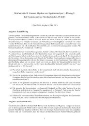
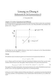
Figure 1 – Four different types of warming commitments. (1) The ‘geophysical’ warming
commitment in case that emissions are abruptly reduced to zero after 2005 (‘Zero Emissions’); Note
that emissions initially rise due to ceased cooling by aerosols. (2) The ‘present forcing’ warming
commitment corresponds to constant radiative forcing at present (2005) levels and comprises the
‘realized’ and ‘unrealized’ warming; (3) the ‘feasible scenario’ warming commitment is the
temperature rise that corresponds to the lowest emission scenario judged feasible. Note that the
mitigation scenario B2-400-MES-WBGU is shown for illustrative purposes only (dash-dotted line:
original scenario up to 2100; dotted part: the extended scenario as described in text). Lastly, (4) the
‘constant emissions’ warming commitment that corresponds to highest warming levels in the long
term. The historical temperature record and its uncertainty (grey shaded area) is taken from Folland
et al. (2001).

WARMING C OMMITMENT 21
2.4 METHOD
This section entails a brief description of the simple climate model MAGICC (2.4.1) employed in this work.
In the non probabilistic components of this work we use a standard ‘7 AOGCM ensemble mean’ (7AEM)
procedure to average over model runs tuned to different AOGCMs (2.4.2). In addition, a probabilistic
procedure allows us to give special attention to uncertainties in the climate’s sensitivity based on a range of
literature estimates (2.4.3). For additional equilibrium calculations standard formulas were applied (2.4.4).
Finally we describe the assumptions made in regard to natural forcings (2.4.5).
2.4.1 SIMPLE CLIMATE MODEL
For the computation of global mean climate indicators, the simple climate model MAGICC 4.1 has been
used 12 . The description in the following paragraph is largely based on Wigley (2003a). MAGICC is the
primary simple climate model that has been used by the IPCC to produce projections of future sea level rise
and global-mean temperatures. Information on earlier versions of MAGICC has been published in Wigley
and Raper (1992) and Raper et al. (1996). The carbon cycle model is the model of Wigley (1993), with further
details given in Wigley (2000) and Wigley and Raper (2001). Modifications to MAGICC made for its use in
the IPCC TAR (IPCC, 2001c) are described in Wigley and Raper (2001; 2002), Wigley et al. (2002) and
(Wigley, 2005). Additional details are given in the IPCC TAR climate projections chapter 9 (Cubasch et al.,
2001). Gas cycle models other than the carbon cycle model are described in the IPCC TAR atmospheric
chemistry chapter 4 (Ehhalt et al., 2001) and in Wigley et al. (2002). The representation of temperature related
carbon cycle feedbacks has been slightly improved in comparison to the MAGICC version used in the IPCC
TAR, so that the magnitude of MAGICC’s climate feedbacks are comparable to the carbon cycle feedbacks
of the Bern-CC and the ISAM model (see Box 3.7 in Prentice et al., 2001) 13 .
The gases that are modeled for each scenario are carbon dioxide (CO 2), methane (CH 4), nitrous oxide (N 2O),
fluorinated gases (HFCs, PFCs, SF 6), and sulphur emissions (SOx) as well as carbon monoxide (CO), volatile
organic compounds (VOC), and nitrogen oxide (NOx). If not otherwise stated, all indicated temperatures are
annual and global mean surface temperature levels above pre-industrial levels (1861-1890)..
2.4.2 AOGCM ENSEMBLE MEAN
Ensemble mean outputs of this simple climate model are the basis for the non-probabilistic results presented
in this study. The ensemble outputs are computed as means of seven model runs. In each run, 13 model
parameters of MAGICC are adjusted to optimal tuning values for seven atmospheric-ocean global circulation
models (AOGCMs) (see Raper et al. (2001). This ‘7 AOGCM ensemble mean’ (7AEM) procedure, which we
will hereafter refer to as 7AEM , is widely used in the IPCC Third Assessment Report and described in
Appendix 9.1 (Cubasch et al., 2001). By using this 7AEM procedure, the implicit assumptions in regard to
climate sensitivity is based on the seven AOGCMs. The mean climate sensitivity for those 7 AOGCMs
models is 2.8°C for doubled CO 2 concentration levels (median is 2.6°C). Clearly, different climate projections
would be obtained, if single model tunings or different climate sensitivities were used, reflecting the
underlying uncertainty in the science.
12 MAGICC 4.1 has been developed by T.M.L. Wigley, S. Raper and M. Hulme and is available at
http://www.cgd.ucar.edu/cas/wigley/magicc/index.html, accessed in May 2004.
13 This improvement of MAGICC only affects the no-feedback results. When climate feedbacks on the carbon cycle are included,
the differences from the IPCC TAR are negligible.

22 M ALTE M EINSHAUSEN, 2005, CLIMATE T ARGETS
2.4.3 HANDLING UNCERTAINTIES: CLIMATE SENSITIVITY
In addition to these 7AEM runs, another approach had to be chosen to deal with the main climate system
uncertainty, the climate sensitivity. The climate sensitivity is simultaneously one of the most fundamental and
uncertain properties of the climate system in relation to policy. Following the convention in the literature it is
defined as the equilibrium increase in global mean surface temperature following a doubling CO 2
concentrations, e.g. doubling of pre-industrial levels (2 x 278=556ppm). Thus, estimates of the climate
sensitivity approximately reflect the equilibrium warming that can be expected under a 550 CO 2 equivalent
stabilization scenario.
There is no single universally agreed estimate of climate sensitivity or even of a probability density function
for it. We have attempted to deal with this uncertainty by making probabilistic calculations for temperature
projected for different probability density functions of climate sensitivity. Whilst varying the climate
sensitivity parameter we have maintained the default set of climate parameters for MAGICC consistent with
the IPCC Third Assessment Report findings (Wigley, 2003a). Specifically, we sampled climate sensitivity at
the quantiles of interest, namely 1%, 5%, 10%, 33% 50%, 66%, 90%, 95% and 99% of the PDFs (cf. Figure 4
and Figure 7).
Clearly, this procedure does not take into account interdependencies between climate sensitivity and other
climate parameters, such as ocean heat diffusion. Ideally, the simple climate model should be run for
parameter sets from a joint probability density distribution for the key uncertainties. We choose to focus only
on climate sensitivity and neglect interdependencies as well as uncertainties in other key climate parameters.
This should be kept in mind when reviewing the results. Neglecting uncertainties in ocean mixing, specifically
the likely lower ocean mixing rates for lower climate sensitivities, might have relatively limited effects
though 14 .
Since its First Assessment Report in 1990, the IPCC has indicated that the climate sensitivity is most likely to
lie in the range 1.5-4.5°C. Prior to the IPCC TAR the IPCC had given a best estimate of 2.5°C. However, in
the TAR no reference was made to a best estimate and instead to an average model range. Hence there is no
real quantitative guidance at this stage arising from the IPCC assessments other than by the “likelihood” of
the climate sensitivity lying in range 1.5°C to 4.5°C.
After the completion of the IPCC TAR, a number of estimates of the climate sensitivity have been published
each with its own strengths and weaknesses (see e.g. IPCC, 2004). Seven of these estimates are used in the
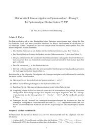
subsequent analysis and shown in Figure 2 15 : Six studies have attempted objective estimation of a probability
density function (PDFs) for climate sensitivity based on contemporary forcing history and the recent
evolution of the climate system: (1) the combined PDF by Andronova and Schlesinger (2001) that takes into
account both solar forcing and sulphate aerosols 16 ; (2-3) estimates by Forest et al. (2002) with expert and
uniform a priori distributions; (4) another observationally based estimate by Gregory et al. (2002); (5) the
uniform prior estimate by Knutti et al. (2003); (6) a recent estimate based on a 53-member ensemble of an
atmosphere GCM, HadAM3, coupled to a mixed layer ocean model to enable integrations to equilibrium
(Murphy et al., 2004). (7) The seventh estimate is drawn from the conventional 1.5°C to 4.5°C IPCC
uncertainty range with a pdf constructed by Wigley and Raper (2001). This estimate assumes that the
distribution is log-normal with the IPCC range being taken as the 90% confidence range. This can be seen as
an attempt to codify the expert judgement character of the IPCC assessments, but, as is emphasized by
14 The projection range for the ‘present forcing’ warming commitment due to the 1.5 to 4.5°C uncertainty range in climate
sensitivity narrows slightly, if a conventional uncertainty range for ocean mixing (1.3 to 4.1 cm 2 /sec, (Wigley, 2005)) is assumed to be
dependent on climate sensitivity. The sensitivity of the simple climate model results to uncertainties in ocean mixing is highest for the
near-term transient climate response and ceases in the long-term equilibrium. Specifically, the uncertainty range narrows in 2050 and
2400 by 18% and 1%, respectively, if the 1.3 (4.1) cm 2 /sec ocean mixing rate is assumed to go hand in hand with a 1.5 (4.5)°C climate
sensitivity in comparison to computing future temperatures by using a medium range 2.3 cm 2 /sec ocean mixing ratio independent of
climate sensitivity. This is generally in line with results by Wigley, who estimated that the effect of ocean mixing uncertainties being
relatively small compared to uncertainties of climate sensitivity and present forcing (Wigley, 2005).
15 Additional estimates of the climate sensitivity and their likely ranges have for example been performed by Harvey and
Kaufmann (2002). However, adding more estimates to the analysis would not have added to the substance of the discussion below.
16 Note, that the conventionally cited ‘combined pdf’ from Andronova & Schlesinger (Andronova and Schlesinger, 2001) has been
combined from estimates that do not take into account aerosol forcing or variations in solar radiation. Therefore, it is not displayed
here.

WARMING C OMMITMENT 23
Wigley and Raper (2001) does not represent either the full range of uncertainty or some “best estimate” based
on all other estimates.
In the following work we have used all of the pdfs described above and to illustrate some of our results we
have chosen to focus on the PDFs (5) to (7) as they span the range of available climate sensitivity PDF
estimates in terms of their shape and methods by which they have been derived (see Figure 2). PDFs (5) and
(6) are based on the recent period but have very different shapes, PDF (7) is roughly similar to the Forest et
al 2002 expert prior estimate but has the virtue for the discussion of results here that it codifies the expert
assessment of the IPCC.
Probability Density (˚C-1)
0.9
0.8
0.7
0.6
0.5
0.4
0.3
0.2
0.1
0
Andronova and Schlesinger (2001) - with sol.&aer. forcing
Forest et al. (2002) - Expert priors
Forest et al. (2002) - Uniform priors
Gregory et al. (2002)
Knutti et al. (2002)
Murphy et al. (2004)
Wigley and Raper (2001) - IPCC lognormal
0 1 2 3 4 5 6 7 8 9 10
Climate Sensitivity (˚C)
Figure 2 - Different estimates of the probability density functions for climate sensitivity.
2.4.4 TIME HORIZON, EQUILIBRIUM CONSIDERATIONS AND CO2 EQUIVALENCE
The time horizon used to explicitly evaluate warming commitments based on defined scenarios here is to the
year 2400. This is arbitrary given that the climate system will continue to respond well beyond this time. As
has been shown the warming following greenhouse gas concentration stabilization will continue for a few
thousand years and only slowly approach equilibrium (Watterson, 2003).
As in the MAGICC climate model, the following formula is used for the presented equilibrium calculations
(see as well Ramaswamy et al., 2001, Table 6.2, page 358). The conversion between CO 2 (equivalence)
concentrations and radiative forcing (Q) (W/m 2 ) follows the logarithmic equation:
Δ Q = α ln C C
0 (1)
where is 5.35 W/m 2 and C 0 the unperturbed pre-industrial CO 2 concentration level (278ppm), based on
Myhre et al. (1998). The equilibrium temperature is then assumed to scale linearly with radiative forcing:
ΔT
Δ T =ΔQ α ln(2)
2xCO2
(2)
where T 2xCO2 (K) is the climate sensitivity and *ln(2) is the radiative forcing for twice the pre-industrial
CO 2 levels.

24 M ALTE M EINSHAUSEN, 2005, CLIMATE T ARGETS
CO 2 equivalent concentrations are here derived from the net forcing of all anthropogenic radiative forcing
agents. Thus, CO 2 equivalence comprises both greenhouse gases and aerosols but not natural forcings.
2.4.5 NATURAL FORCINGS
Historic solar and volcanic forcings estimates have been assumed, according to Lean et al. (1995) and Sato et
al. (1993) respectively, as presented in the IPCC TAR (see Figure 6-8 in Ramaswamy et al., 2001). Recent
studies suggested that an up-scaling of solar forcing might lead to a better agreement of historic temperature
records (e.g. Hill et al., 2001; North and Wu, 2001; Stott et al., 2003). In accordance with the best fit results
by Stott et al. (2003, table 2), a solar forcing scaling factor of 2.64 has been assumed for this study.
Accordingly, volcanic forcings from Sato et al. (1993) have been scaled down by a factor 0.39 (Stott et al.,
2003, table 2). Future solar and volcanic forcings over the future time periods examined here have been
assumed constant at levels equivalent to the scaled mean forcings over the past 22 and 100 years respectively.
In other words, we have assumed a scaled solar forcing of +0.44W/m 2 and -0.14W/m 2 for volcanic forcing,
which is together 0.67W/m 2 above the natural forcing of the 1861-1890 period 17 .
It should be noted that mechanisms for the amplification of solar forcing are not yet well established
(Ramaswamy et al., 2001, section 6.11.2; Stott et al., 2003). As well, the evidence for the conventionally
assumed long-term solar irradiance changes has recently been challenged (Foukal et al., 2004).
An exception to the above solar and volcanic forcing assumptions has been made for the calculations on the
risk of overshooting certain temperature levels in equilibrium (section 2.5.5). There, equilibrium temperatures
have been directly derived from anthropogenic radiative forcings. Thus, natural forcings have implicitly been
assumed constant at pre-industrial levels. This approach allows separating risks that solely accrue from human
interference and those that accrue from changes in natural forcings. Assuming no change of natural forcings
since pre-industrial times will lower the presented temperature increase by 0.35°C in equilibrium for the
7AEM runs (see Table I, Table II and Table III). Thus, it should be noted that the presented overshooting
risks are lower than if the above standard assumptions on natural forcings were applied.
17 The alternative, to leave natural forcings out in the future, is not really viable, since the model has been spun up with estimates
of the historic solar and volcanic forcings. Assuming the solar forcing to be a non-stationary process with a cyclical component and
assuming that the sum of volcanic forcing events can be represented as a Compound Poisson process, it seems more realistic to apply
the recent and long-term means of solar and volcanic forcings, respectively, for the future. Note as well endnote 9.

WARMING C OMMITMENT 25
2.5 RESULTS:THE WARMING COMMITMENTS AND AVOIDABLE WARMING
Below we first outline the results of the analysis for the warming commitments based on the four concepts
outlined at the beginning of the paper (Sections 2.5.1 to 2.5.4). We then provide a compilation of results by
deriving the probability that we are already ‘committed’ to overshoot certain warming levels (2.5.5). Finally,
we present estimates of the scale of avoidable warming by analysing paired mitigation and non-mitigation
scenarios (2.5.6).
2.5.1 CONSTANT EMISSIONS
If greenhouse gas and aerosol emissions were held constant at present day (2005) levels, the associated
radiative forcing would rise markedly in the future. By inverting equation 1 the total radiative forcing can be
expressed in equivalent CO 2 concentrations – the CO 2 concentration which would produce that level of
radiative forcing if acting alone. In CO 2 equivalent terms the radiative forcing would rise to 527ppm CO 2eq
by 2100 and 899ppm CO 2eq by 2400 (excl. natural forcing). For comparison the actual CO 2 concentration
would rise up to 531ppm by 2100 and 929ppm by 2400. The relatively small difference between CO 2 and
CO 2eq is due to the offsetting effects of aerosol. A central estimate is that at the global mean level the direct
and indirect aerosol cooling effects are sufficient to approximately counteract the warming effects of the non-
CO 2 well mixed greenhouse gases. Temperature would increase monotonically up to 4.2°C in 2400 (2.0°C in
2100) – according to the 7AEM results. Assuming lower (1.5°C) and higher (4.5°C) climate sensitivities, the
temperature range in 2400 spans from 2.5°C to 6.1°C, respectively (2100: 1.4°C to 2.7°C) 18 . The 90%
confidence ranges for global mean temperatures based on climate sensitivity estimates by Murphy et al. (2004)
is 1.9°C to 3.0°C in 2100 and 3.7°C to 7.0°C by 2400. See Table I for further estimates for different climate
sensitivity PDFs.
Figure 4 is an example of a probabilistic assessment of warming resulting from constant emissions (and other
cases) using the climate sensitivity pdfs outlined earlier. In this figure are shown the 1%, 10%, 33%, 66%,
90% and 99% percentiles for warming estimates based on the IPCC range as codified by Wigley and Raper
(2001).
18 Note that there are corresponding slight variations in CO2 concentrations across the different climate sensitivities due
to climate feedbacks on the carbon cycle. For a climate sensitivity of 1.5°C (4.5°C), CO2 concentration in 2400 will be
900 (960) ppm.

26 M ALTE M EINSHAUSEN, 2005, CLIMATE T ARGETS
Table I - 'Constant emission' warming commitment: temperature implications in the case where
emissions are held constant at today’s (2005) levels. Results are given for the 7AEM as well as the
probabilistic calculations based on different estimates of climate sensitivity PDFs by Wigley &
Raper (2001), Murphy et al. (2004), and Knutti et al. (2003). In addition, equilibrium temperatures for
2400 forcing levels are given with applying the standard natural forcing assumptions (EQUI w NF)
and without assuming any natural forcing changes from pre-industrial levels (EQUI w/o NF).
Temperature above pre-industrial
(°C above pre-industrial)
Climate
2000 2005 2050 2100 2200 2400
Sensitivity
7 AOGCM ensemble mean
EQUI
w NF
EQUI
w/o NF
~2.8 0.7 0.8 1.5 2.0 2.9 4.2 5.2 4.9
Wigley
5%: 1.50 0.5 0.6 1.0 1.4 1.8 2.5 2.7 2.6
50%: 2.60 0.6 0.8 1.4 2.0 2.8 4.0 4.8 4.5
95%: 4.50 0.7 0.9 1.9 2.7 4.1 6.1 8.5 7.9
Murphy
5%: 2.40 0.6 0.7 1.4 1.9 2.6 3.7 4.4 4.1
50%: 3.42 0.7 0.8 1.7 2.3 3.4 5.0 6.4 6.0
95%: 5.37 0.8 0.9 2.0 3.0 4.6 7.0 10.2 9.5
Knutti
5%: 1.47 0.5 0.6 1.0 1.3 1.8 2.5 2.7 2.5
50%: 4.33 0.7 0.9 1.9 2.7 4.0 6.0 8.1 7.6
95%: 9.28 0.9 1.1 2.5 3.9 6.2 >8 18.1 17.0
2.5.2 THE ‘PRESENT FORCING’ WARMING COMMITMENT
One of the scenarios often used to convey a sense of inertia and of committed warming to policy makers is
that of holding radiative forcing constant from a certain point in time.
The Hadley Centre, for example, recently estimated the additional warming that would follow from
stabilization of greenhouse gas concentrations at present levels (see thick dotted line in panel c of Figure 3).
The total warming above pre-industrial by 2100 was estimated by about 1.1°C with an ultimate warming of
1.6°C over many centuries (Hadley Centre, 2002, p. 3, 2003, p. 12). Other models yield similar estimates when
holding radiative forcing constant (Meehl et al., 2005; Wigley, 2005). Using a climate model with higher
sensitivity (3.7°C) than in the Hadley Centre analysis, the results of Wetherald et al. (2001) 19 indicate a total
warming at equilibrium of around 2.1°C above 1861-1890 would occur with forcing held constant at year
2000 levels 20 .
In this study, results suggest an increase of global mean surface temperatures by about 0.4°C up to 2400 over
the observed 2002 levels (1.2°C above pre-industrial), if radiative forcing were held fixed at present levels
(estimated to be 1.93 W/m 2 including natural forcings in 2005) (7AEM ). In equilibrium, temperatures are
estimated to rise up to 1.5°C above pre-industrial values if assumptions on current natural forcing continue to
19 The GFDL R15 model of (Manabe et al., 1991) was used and has a climate sensitivity in its mixed layer form of 3.7°C and in
the full coupled version 4.5°C (Stouffer and Manabe, 1999). The committed warming has been calculated as the year 2000 difference
of the mixed layer equilibrium model run and the transient AOGCM.
20 This warming is the total reported from the equilibrium mixed layer (EML) model from 1760 and adjusted downwards by 0.2°C
in order to ensure consistency with the here used base period from 1861-1890 (cf. Figure 1 of Wetherald et al, (2001).

WARMING C OMMITMENT 27
apply. If no change of natural forcing since pre-industrial times were assumed, the equilibrium warming
would be about 0.35°C lower, namely 1.2°C.
Running the simple climate model with default IPCC TAR parameter settings, but the IPCC bounds of
climate sensitivity (1.5°C and 4.5°C), the 2400 total warming lies between 0.8°C and 1.7°C. At equilibrium
the warming range would be 0.8 to 2.4°C (cf. Table II).
It should be kept in mind that the present forcing is dampened greatly by the cooling effect of aerosols that
counteracts the warming effect of greenhouse gases, although the magnitude is uncertain. Thus, the present
forcing warming commitment might be up to 1.9 (2.1) °C by 2100 (2400) for the 7AEM , if it is assumed that
SO 2 aerosol emissions were to cease, but greenhouse gas concentrations remain at the current level (452ppm
CO 2 equivalence) 21 .
Table II - 'Present forcing' warming commitment: temperature implications in case that radiative
forcing is held constant at today’s (2005) levels (368ppm CO 2 equivalence). Otherwise as Table I.
Climate
Sensitivity
Temperature above pre-industrial
(°C above pre-industrial)
2000 2005 2050 2100 2200 2400
EQU
I w
NF
EQU
I w/o
NF
7 AOGCM ensemble mean
~2.8 0.7 0.8 1.0 1.1 1.1 1.2 1.5 1.2
Wigley
5%: 1.50 0.5 0.6 0.7 0.7 0.8 0.8 0.8 0.6
50%: 2.60 0.6 0.7 0.9 1.0 1.1 1.1 1.4 1.1
95%: 4.50 0.7 0.9 1.2 1.4 1.5 1.7 2.4 1.9
Murphy
5%: 2.40 0.6 0.7 0.9 1.0 1.0 1.1 1.3 1.0
50%: 3.42 0.7 0.8 1.1 1.2 1.3 1.4 1.8 1.4
95%: 5.37 0.8 0.9 1.3 1.5 1.7 1.9 2.9 2.2
Knutti
5%: 1.47 0.5 0.6 0.7 0.7 0.8 0.8 0.8 0.6
50%: 4.33 0.7 0.9 1.2 1.3 1.5 1.7 2.3 1.8
95%: 9.28 0.9 1.1 1.7 2.0 2.3 2.8 5.0 3.9
21 Note that there is significant uncertainty in regard to the aerosols’ cooling effect. This greenhouse gas only CO 2 equivalence
level has been derived from the 2005 radiative forcing when running the SRES A1B emission scenario with zeroed SO 2 emissions
under the 7AEM procedure.

28 M ALTE M EINSHAUSEN, 2005, CLIMATE T ARGETS
1000
Concentration (ppmv)
800
600
400
a) CO 2
constant emissions
constant forcing
zero emissions
Concentration (ppmv)
1000
800
600
400
b) CO 2 equivalent
constant emissions
constant forcing
6.8
5.7
4.1
1.9
Rad. Forcing (W/m 2 )
zero emissions
˚C above pre-industrial
4
3
2
1
c) Temperature
@ 7 AOGCM ensemble mean
observed
CCSM3
constant emissions
Hadley
constant forcing
zero emissions
0
1900 2000 2100 2200 2300 2400
Figure 3 - Effects of abrupt cessation of emissions, constant radiative forcing, and constant
emissions from 2005 onwards (a) CO 2 concentrations, (b) CO 2 equivalent concentrations and
radiative forcing, (c) global mean surface temperature. Shown are results of the ‘7 AOGCMs
ensemble mean’ runs with an approximate climate sensitivity of 2.8°C. In addition, the 20 th warming
commitment results are plotted for the CCSM3 model runs (Meehl et al., 2005) (grey solid lines).
The Hadley centre’s estimate of the warming commitment related to a constant radiative forcing
(dotted grey line in panel c) (Hadley Centre, 2002) is approximately equivalent to the 7AEM one
derived here. All temperature model runs are calibrated towards the 1961-1990 observational record
data from (Folland et al., 2001), shown with uncertainties (grey band with black solid line).

WARMING C OMMITMENT 29
Global Mean Temperature
(C˚ above pre-industrial)
5
4
3
2
1
a) Constant
b) Present Forcing
c)
Emissions
Zero Emissions
0
1900 2000 2100 2200 2300 24001900 2000 2100 2200 2300 2400 1900 2000 2100 2200 2300 2400
Figure 4 - Global mean temperature increase in case that emissions are held constant at 2005 levels
(left a,d), that radiative forcing is held constant (middle b,e) or that emissions are abruptly reduced
to zero (right c,f). Likelihood ranges are given for the lognormal fit to the conventional 1.5-4.5°C
IPCC range (Wigley and Raper, 2001): the 90% confidence range (dashed lines), the median
projection (solid line), as well as the 1%, 10%, 33%, 66%, 90% and 99% percentiles (borders of
shaded areas).
2.5.3 THE ‘GEOPHYSICAL’ WARMING COMMITMENT AND ITS INCREASE OVER
TIME
A complete and abrupt cessation of human emissions would soon reverse the increase in radiative forcing
and result in a halt to global mean temperature. However, in the beginning, the cessation of sulphur emissions
causes a short, but pronounced, increase in net radiative forcing and temperatures (Wigley, 1991). Within a
decade temperatures would be begin to fall, though (Figure 3.c). Until at least 2100 it seems likely that
temperature levels at least as high as year 2000 levels would prevail, even if all human-induced emissions were
to be halted today. However, beyond 2100, there is no geophysical commitment to a further increase in
warming, but there is a floor to how fast temperatures can drop 22 . The indicated lower bound of
approximately 0.3°C to 0.4°C results largely from the increase in solar forcing since pre-industrial times and
assumed continuation of current levels (see section 2.4.5). CO 2 concentrations would fall slowly and approach
levels that were found at the beginning of the 20 th century towards the end of the 22 nd century, namely
300ppm (see Figure 3.a). The slow take up of the airborne fraction of anthropogenic carbon emissions by the
oceans determines the rates of temperature reduction in the 22 nd century and beyond and also ultimately
determines the rise in sea level.
In order to see how the geophysical warming commitment increases with time, we have shown the effects of
emissions being switched off at six ten-year intervals from 2001 to 2051 for the SRES A1B scenario on global
mean temperature. This may help place lower bounds on the costs of delaying policy action (see section
2.6.2). The additional ‘warming commitment’ by 2100 increases by about 0.2-0.3°C for each 10-year delay and
over the period to 2400 by 0.1-0.2°C (see Table IV and Figure 5).
22 One potential technique for increasing the rate of CO2 removal from the atmosphere beyond its natural limits could be
biomass burning with subsequent capture and storage of CO2 in the flue gas (Azar et al., submitted).

30 M ALTE M EINSHAUSEN, 2005, CLIMATE T ARGETS
Table III - 'Geophysical' warming commitment: temperature implications in case that all emissions
are ceased from 2005. Otherwise as Table I.
Temperature above pre-industrial
(°C above pre-industrial)
Climate
EQUI w EQUI
2000 2005 2050 2100 2200 2400
Sensitivity
NF w/o NF
7 AOGCM ensemble mean
~2.8 0.7 0.8 0.9 0.7 0.6 0.4 0.4 0.1
Wigley
5%: 1.50 0.5 0.7 0.6 0.5 0.4 0.3 0.2 0.0
50%: 2.60 0.6 0.8 0.8 0.7 0.5 0.3 0.4 0.1
95%: 4.50 0.7 1.0 1.2 1.0 0.7 0.5 0.7 0.1
Murphy
5%: 2.40 0.6 0.8 0.8 0.7 0.5 0.3 0.3 0.1
50%: 3.42 0.7 0.9 1.0 0.8 0.6 0.4 0.5 0.1
95%: 5.37 0.8 1.0 1.3 1.1 0.8 0.6 0.8 0.2
Knutti
5%: 1.47 0.5 0.7 0.6 0.5 0.4 0.3 0.2 0.0
50%: 4.33 0.7 1.0 1.1 0.9 0.7 0.5 0.6 0.1
95%: 9.28 0.9 1.2 1.6 1.5 1.2 0.9 1.5 0.4
Table IV – The geophysical warming commitment over time (columns) is depending on the year,
when emissions are reduced to zero (rows). Before being ceased, emissions were assumed to follow
the SRES A1B-AIM baseline scenario (cp. Figure 5). Results are shown for the ‘7 AOGCM ensemble
mean’ and equilibrium values with and without natural forcing (‘EQUI w NF’ and ‘EQUI w/o NF’,
respectively).
Temperature above pre-industrial
(°C above pre-industrial)
Ceasing
205 210 220 240 EQUI EQUI
2000 2005
emissions
0 0 0 0 w NF w/o NF
2001 0.7 1.1 0.8 0.7 0.5 0.3 0.4 0.0
2011 0.7 0.7 1.0 0.8 0.6 0.4 0.5 0.1
2021 0.7 0.7 1.3 1.0 0.8 0.6 0.6 0.3
2031 0.7 0.7 1.7 1.3 1.0 0.7 0.8 0.4
2041 0.7 0.7 2.1 1.6 1.2 0.9 0.9 0.6
2051 0.7 0.7 2.2 1.9 1.4 1.1 1.1 0.8

WARMING C OMMITMENT 31
(ppmv)
700
600
500
400
a) CO 2 concentrations
Ceasing Emissions:
2051
2041
2031
2021
2011
2001
(ppmv)
300
700
600
500
400
300
b) CO 2 equivalent
concentrations
4.94
4.16
3.14
1.95
0.41
Rad. Forcing (W/m2)
(˚C above pre-industrial)
2
1
0
c) Temperature
@ 7 AOGCM ensemble mean
Figure 5 - Effects of 10 year lags in reducing emissions to zero on (a) CO 2 concentrations, (b) CO 2
equivalent concentrations and radiative forcing, (c) global mean temperature. Emissions are
reduced to zero in 2001, 2011,..,2051 after following the SRES A1B-AIM scenario.
2.5.4 THE ‘FEASIBLE SCENARIO’ WARMING COMMITMENT
We now turn to an examination of what the warming commitment might be for a range of feasible emissions
scenarios. We use explicit scenarios from the literature that produce a range of different radiative forcing
pathways (see section 2.3.4). If not otherwise indicated, all results below refer to the 7AEM results (see
section 2.4.2). Furthermore, we examine the equilibrium warming when forcing is stabilized at a range of CO 2
equivalent levels (see method’s section 2.4.4).
For the period up to 2100, the 450ppm CO 2 scenarios result in a warming in the range of 2.2-2.4°C above
pre-industrial levels (7AEM ). An exception is the A1FI-450 MiniCam scenario that results in higher warming
(3.0°C) due to very high unabated N 2O emissions. For the two 400ppm scenarios the range is 1.9-2.1°C in
2100. The 350ppm CO 2 stabilization scenarios of Azar et al. (submitted) yield a warming of about 1.5-1.7°C

32 M ALTE M EINSHAUSEN, 2005, CLIMATE T ARGETS
by 2100 23 . In contrast, temperatures in 2100 will increase to levels that are between 2.5°C to 4.8°C above preindustrial
ones, if emissions were to follow one of the non-mitigation scenarios analysed here (see Figure 6).
In summary, if the 350ppm and 400ppm CO 2 scenarios were considered to represent the outer limit of where
climate policies can reach, we would be committed to an additional warming of 0.7 to 1.3°C above the
warming of 0.8°C in 2003 (Folland et al., 2001; Jones and Moberg, 2003).
The period beyond 2100 is critical to warming commitment assessments. However, published mitigation
scenarios are generally limited to 2100. Therefore, we have extended these scenarios so that they stabilize
CO 2 concentrations at the indicated levels. For example, the WBGU B2-400 MESSAGE scenario is extended
so that CO 2 concentrations stabilize at 400ppm. The emissions of other greenhouse gases and aerosols
beyond 2100 are assumed to correlate with the extended fossil CO 2 emissions in a specific way, namely by
making use of the 2100 emission characteristics of 54 SRES and post-SRES scenarios via the ‘Equal Quantile
Walk’ method (see Chapter 0). A special case is the AZAR-350-BECS scenario, where the fossil CO 2
emissions are negative (-3.6 GtC/yr) in 2100 and assumed to smoothly return to zero by 2200. As a
consequence, CO 2 concentrations will stabilize at about 310ppm and CO 2 equivalent concentrations at about
350ppm by 2150 (see Table V).
By 2400, temperatures would have risen to 1.5°C, 2.0°C and 2.4°C for the 350ppm, 400ppm and 450ppm
CO 2 stabilization scenarios, respectively, according to the ‘7AEM ’. Temperatures for the AZAR-350-BECS
scenario, which is assumed to stabilize at the lowest CO 2 level of 310ppm, would have returned to about
1.2°C by 2400 (see Figure 6).
The risk of overshooting 2°C is about 66% for the 450 CO 2 scenarios (500 CO 2eq) (Figure 7 a),
approximately 33% for the 400ppm CO 2 scenarios (440ppm CO 2eq) (Figure 7 b), and 33% around the peak
and 2% in the long-term for the analysed 310ppm CO 2 scenario AZAR-350-BECS (350ppm CO 2eq)
(Figure 7 c; cf. Table V for risks in equilibrium without natural forcing).
2.5.5 RISK OF OVERSHOOTING CERTAIN WARMING LEVELS IN EQUILIBRIUM
The warming commitments shown for the scenarios extend to 2400 and are not the final warming of the
system if these concentration levels are maintained (Watterson, 2003). It is instructive therefore to examine
the final committed warming in equilibrium. Taking into account the uncertainty in the climate sensitivity, we
present probabilistic results in terms of the risks that certain temperature thresholds (1.5°C to 3.5°C) are
overshot (see Table V). The estimates we present here constitute a lower bound estimate, if stabilization
levels are approached ‘from above’, i.e. after concentration peaked at higher levels before returning to the
ultimate stabilization level (cf. Figure 7 c). For the higher stabilization scenarios, risk might be lower in
practice, if concentration levels were not stabilized, but continuously decreased after 2100. This would
prevent the full equilibrium warming from being realized. It should be kept in mind that natural forcings are
here not taken into account (see section 2.4.5).
23 As aforementioned (section 2.3.4), the non-CO2 emissions for the Azar scenarios are here drawn from the WBGU B2-400
scenario. Thus, temperature levels in 2100 could be slightly lower by a few tenths of a degree, if additional non-CO2 emission
reductions were assumed below the ones of the WBGU B2-400 scenario.

WARMING C OMMITMENT 33
Concentration (ppm)
1000
900
800
700
600
500
400
1000
a) CO 2 1a
900
b) CO 2 equivalence
300
1900 2000 2100 2200 2300 2400
(˚C above 1861-1890)
4
3
2
1
3a
3b
1c
1b
2a
1c
1d
2b
1e
1a
1d 1b
1e
2b
2a
1a
1b
2a
1c
1d
2b
3c
1e
1c 1e 1d
2b
2a
3a
3b
PF
1a
1b
3c
PF
c) Temperature
@ 7AOGCM ensemble mean
0
1900 2000 2100 2200 2300 2400
Concentration (ppm)
800
700
600
500
400
6.85
6.29
5.65
4.94
4.12
3.14
1.95
300
0.41
1900 2000 2100 2200 2300 2400
Non-mitigation:
1a
1b
1c
1d
1e
2a
2b
A1FI-MI
A1B-AIM
A1T-WBGU
A1T-MES
B1-IMA
B2-WBGU
B1-WBGU
PF
1b
1c
1d
2b
1e
1d
1c 1e
1b
1a
2b
3a
2a
3b
PF
2a
3c
1a
1b
1c
1d
1e
2a
2b
3a
3b
3c
Mitigation:
A1FI-450-MI
A1B-450-AIM
A1T-450-WBGU
A1T-450-MES
B1-450-IMA
B2-400-WBGU
B1-400-WBGU
AZAR-350-NC
AZAR-350-FC
AZAR-350-BECS
Present forcing commitment
Radiative Forcing (W/m2)
Figure 6 - The climatic effects of a range of SRES non-mitigation scenarios (dotted line) and 350-
450ppm CO 2 stabilization scenarios (solid lines) on (a) CO 2 concentrations, (b) CO 2 equivalent
concentration and radiative forcing, (c) global mean. For comparison, the ‘constant present forcing’
run is plotted as in Figure 3.
Global mean Temperature
(˚C above pre-industrial)
5
4
3
2
1
a) 450 CO2/ 500 CO2eq
b) 400 CO2 / 440 CO2eq
c)
(here: A1T-450-MES)
(here: B2-400-WBGU)
310 CO2/ 350 CO2eq
(here: AZAR-350-BECS)
0
1900 2000 2100 2200 2300 2400 2000 2100 2200 2300 2400 2000 2100 2200 2300 2400
Figure 7 - Temperature increase for mitigation scenarios stabilizing CO 2 at 450ppm (a), 400ppm (b)
and 310ppm CO 2 (c). The CO 2 equivalent concentrations in 2400 are about 500, 440 and 350ppm,
respectively (cf. Figure 6). Otherwise as Figure 4: The underlying climate sensitivity PDF is based
on the conventional 1.5°C to 4.5°C range (Wigley and Raper, 2001).

34 M ALTE M EINSHAUSEN, 2005, CLIMATE T ARGETS
Probability of overshooting 2˚C warming
100%
90%
80%
70%
60%
50%
40%
30%
20%
10%
Radiative forcing (W/m2)
1.23 1.95 2.58 3.14 3.65 4.12 4.54 4.94 5.31
Year 2000
Andronova and Schlesinger (2001) - with sol.&aer. forcing
Forest et al. (2002) - Expert priors
Forest et al. (2002) - Uniform priors
Gregory et al. (2002)
Knutti et al. (2002)
Murphy et al. (2004)
Wigley and Raper (2001) - IPCC lognormal
0%
350 400 450 500 550 600 650 700 750
CO2 equivalence stabilization level
very
likely
likely
medium
likelihood
very
unlikely
unlikely
Probability of overshooting 2˚C (IPCC Terminology)
Figure 8 – Risk of overshooting a 2°C target. Current estimates of the climate sensitivity suggest that
only by stabilizing anthropogenic radiative forcing at levels below 400 or 450ppm CO 2 equivalent
concentrations, the risk of overshooting the 2°C target can be termed “unlikely”. The actual 2000
forcing range and its uncertainty (upper left bar) is taken from Knutti et al. (2002), with the grey
square indicating this study’s present (2005) forcing assumption.

WARMING C OMMITMENT 35
Given contemporary policy discussions around warming limits of 2°C (European Community, 1996; Caldeira
et al., 2003) 5 we focus here on the probability that committed warming will lie above 2°C for different long
term stabilization levels. From Figure 8, it can be seen that the choice of PDF for climate sensitivity
uncertainty is quite fundamental in determining the probability of whether or not 2°C is already committed to
for stabilization scenarios. The Knutti et al. (2002) and Gregory et al. (2002) PDFs with their long high tails
imply the lowest probability to stay within the 2°C limit for the lower concentration levels. In contrast, the
Forest et al. (Forest et al., 2002) estimate that is based on a confined expert a priori PDF suggests a narrower
distribution and a lower mean estimate of climate sensitivity. Thus, according to the Forest et al. “expert
prior” PDF, the risk of overshooting 2°C enters the “unlikely” range around 475ppm CO 2 equivalent
stabilization level and is further reduced to “very unlikely” below the 410ppm CO 2 equivalent stabilization
level 24 .
For stabilization of greenhouse gas concentrations at 550ppm CO 2 equivalent, (corresponding approximately
to a 475ppm CO 2 stabilization), the risk of overshooting 2°C is very high, namely between 68%-99%, with a
mean of 85% across the different climate sensitivity PDFs 25 . In other words, the probability that warming will
exceed 2°C could be categorized as ‘likely’ using the IPCC WGI Terminology. If greenhouse gas
concentrations were to be stabilized at 450ppm CO 2 equivalent then the risk of exceeding 2°C would be
lower, but still significant, in the range of 26% to 78% (mean 47%). This could roughly be categorized as
having a “medium likelihood”. The 450ppm CO 2eq stabilization level would correspond roughly to the
400ppm CO 2 scenarios discussed above. Only for stabilization levels of 400ppm CO 2 equivalent and below,
the possibility that warming of more than 2°C will occur, could be classified as “unlikely” (range 2% to 57%
with mean 27%). The risk of exceeding 2°C in equilibrium is further reduced, namely to 0% to 31% (mean
8%), if greenhouse gases were stabilized at a 350ppm CO 2 equivalent level (see Figure 8).
Again, the question of how much risk of overshooting 2°C we are committed to primarily depends on the
applied definition of a ‘warming commitment’. Firstly, under a ‘constant emission’ scenario there is basically
no chance (at best 2%, cf. Table V) to stay below 2°C in equilibrium. Secondly, the ‘present forcing warming
commitment’ implies a 3% to 43% risk of overshooting 2°C – depending on the assumed climate sensitivity
probability distribution function. When assuming the Murphy et al. (2004) climate sensitivity, the risk is about
8%. Thirdly, the ‘geophysical warming commitment’ with zero emissions does not entail any risks to
overshoot 2°C in equilibrium, since it implies that radiative forcing levels will return to near pre-industrial
levels in the long term. Fourthly, quantification of the ‘feasible scenario warming commitment’ again greatly
depends on whether a 500ppm CO 2 equivalent or rather a 350ppm CO 2 equivalence scenario are considered
the lowest feasible mitigation options. For the climate sensitivity PDF that is based on the conventional IPCC
range (Wigley and Raper, 2001), the probability that we are committed to 2°C in equilibrium range from a
medium likelihood (60%) to exceptionally unlikely (1%) (see Table V).
24 If not otherwise noted, this study follows the terminology introduced by the IPCC TAR WGI for presenting likelihoods in its
Summary for Policymakers: Virtually certain (>99%), very likely (90%-99%), likely (66%-90%), medium likelihood (33%-66%),
unlikely (10%-33%), very unlikely (1%-10%), exceptionally unlikely (

36 M ALTE M EINSHAUSEN, 2005, CLIMATE T ARGETS
Table V - Risk of overshooting different global mean temperatures in equilibrium for the analyzed
warming commitments (rows). In the first two rows, the CO 2, and CO 2 equivalent concentrations are
given for 2400. The risk of overshooting a certain temperature limit in equilibrium (excluding natural
forcings) is given for four climate sensitivity PDF estimates by ‘Wigley’ et al., ‘Murphy’ et al., and
‘Knutti’ et al. (see section 2.4.3). Values in bold indicate risks of less then 33%, termed by IPCC as
‘unlikely’. For example, only if future CO 2 equivalent concentrations are stabilized below 400ppm,
overshooting 2°C in equilibrium is ‘unlikely’ (risk below 33%) for three out of the four climate
sensitivity PDFs.
Warming commitment
1.Constant 2.Present 3.Zero
4. Feasible scenarios
emissions forcing emissions a b c d
CO2 in 2400 (ppm) 929 377 298 450 400 350 310
CO2eq in 2400 (ppm) 899 368 282 500 440 385 350
Risk of overshooting warming level (%)
Wigley 100 14 0 87 65 26 6
Murphy 100 37 0 100 97 60 17
>1.5°
C
>2°C
>2.5°
C
>3°C
>3.5°
C
Knutti 100 59 0 91 82 66 50
Wigley 99 3 0 60 32 7 1
Murphy 100 8 0 95 69 18 3
Knutti 98 43 0 81 69 50 33
Wigley 96 0 0 34 12 1 0
Murphy 100 2 0 73 33 5 1
Knutti 95 30 0 70 57 38 20
Wigley 87 0 0 17 4 0 0
Murphy 100 1 0 43 13 2 0
Knutti 91 19 0 61 47 27 9
Wigley 75 0 0 8 2 0 0
Murphy 99 0 0 21 5 1 0
Knutti 86 10 0 52 38 18 0
2.5.6 AVOIDABLE WARMING
Avoidable warming is computed here on the basis of paired comparisons of mitigation and non-mitigation
scenarios drawn from the range used in evaluating ‘feasible scenario’ warming commitments. Here we have
compared the computed effects on global mean temperature between the SRES non-mitigation scenarios and
the post SRES and/or WBGU 450 and 400ppm CO 2 mitigation scenarios. We compute the global mean
temperature differences between the non-mitigation and mitigation scenario of the same scenario family until
the year 2100. As a lower bound of the expected climate benefits, the ‘current avoidable warming’ indicates
the warming difference in a specific year. The ‘equilibrium avoidable warming’ refers to the equilibrium
warming difference that corresponds to forcing differences in a specific year (see Figure 10).
2.5.6.1 Current avoidable warming
The climate benefits of mitigation scenarios can be correlated to the mitigation effort, here indexed by the
avoided cumulative fossil CO 2 emissions in any given year (see equation 3). The analysis shows that there is a
significant temperature benefit (0.12-0.50°C) in most cases by 2050 based on the 7AEM climate simulations
(see Figure 9). The benefits increase to a range of 0.13°C-0.60°C for higher climate sensitivity (4.5°C) and
decrease to a range of 0.10°C-0.33°C for lower sensitivity (1.5°C). Note that for the B1 IMAGE scenarios the

WARMING C OMMITMENT 37
450ppm CO 2 scenario is warmer than the reference case by about 0.2°C in 2050, which is due to the
reductions of sulphur emissions in the 450ppm CO 2 scenario.
Temperature increase
(˚C above pre-industrial)
@ 7 AOGCM ensemble mean
5
4
3
2
1
0
a
B1-450-IMAGE
B1IMA
B1-400-MES-WBGU
B1MES-WBGU
Year 2050
A1T-450-MES
A1TMES
B2-400-MES-WBGU
B2MES-WBGU
A1T-450-MES-WBGU
A1TMES-WBGU
A1B-450-AIM
A1BAIM
A1FI-450-MiniCAM
A1FIMI
b
B1-450-IMAGE
B1IMA
B1-400-MES-WBGU
B1MES-WBGU
Year 2100
A1T-450-MES
A1TMES
B2-400-MES-WBGU
B2MES-WBGU
A1T-450-MES-WBGU
A1TMES-WBGU
A1B-450-AIM
A1BAIM
A1FI-450-MiniCAM
A1FIMI
2000
c
d
A1FIMI
Cumulative emissions
(fossil CO2 as GtC since 2005)
1500
1000
500
0
B1-450-IMAGE
B1IMA
B1-400-MES-WBGU
B1MES-WBGU
A1T-450-MES
A1TMES
B2-400-MES-WBGU
B2MES-WBGU
A1T-450-MES-WBGU
A1TMES-WBGU
A1B-450-AIM
A1BAIM
A1FI-450-MiniCAM
A1FIMI
B1-450-IMAGE
B1IMA
B1-400-MES-WBGU
B1MES-WBGU
A1T-450-MES
A1TMES
B2-400-MES-WBGU
B2MES-WBGU
A1T-450-MES-WBGU
A1TMES-WBGU
A1B-450-AIM
A1BAIM
A1FI-450-MiniCAM
Figure 9 – Comparison of cumulative emissions and temperature increase for 2050 and 2100. The
non-mitigation scenarios (black bars) have higher cumulative emissions (c,d) than the mitigation
scenarios (grey bars). Consequently, the ‘current’ temperature increase up to year 2050 and 2100 is
lower for almost all mitigation scenarios (cf. Figure 10). The 7AEM procedure has been applied here
(cf. section 2.4.2).

38 M ALTE M EINSHAUSEN, 2005, CLIMATE T ARGETS
It can be seen that the further one goes into the future the larger is the benefit of climate policy - with the
benefit strongly associated with the scale of the mitigated emissions. In the 7AEM computations presented
here, the avoided warming at any year is about 0.16 °C for each 100 GtC avoided cumulative fossil CO 2
emissions until that year (see equation 3). Statistical analysis of existing multi-gas mitigation and nonmitigation
scenarios suggests the following regression relationship for a climate sensitivity of about 2.8°C
(‘7AEM ’):
t
0.16°
C
Δ T
current, t
= * Ei
100GtC i =
Δ
(3)
2000
with
Ei : Difference in fossil CO 2 emissions in year i between the unmitigated and mitigated cases as index of the (multi-gas)
mitigation effort.
T current, t : Difference in temperature in year t. between the unmitigated and mitigated cases.
As in the case of equation (4), the regression coefficients are estimated from warming and cumulative
emission differences between the non-intervention and intervention scenario variants in 2050, 2075, and 2100
(see Figure 10). A higher or lower climate sensitivity would produce a higher or lower temperature scaling
factor in equations (3) and (4) 26 .
2.5.6.2 Avoidable warming in the longer term
Note that the ‘current’ avoidable warming relation is a conservative lower bound estimate of the climate
benefits of mitigation. The avoided warming due to fossil CO 2 emissions avoided up to specific year t, e.g.
2050, 2075 or 2100, will grow beyond that year due to the inertia of the climate system. This effect is not fully
captured by comparing avoided warming and avoided emissions for the same year, as presented in the
previous section. Therefore, we present as well the equilibrium benefits of mitigation. The equilibrium
benefits are computed as the difference of equilibrium warming that correspond to the forcing of the
mitigation and non-mitigation scenario in a specific year. The avoided emission are the integral of the
difference between the unmitigated and mitigated emissions scenarios from the base year until a specific year
t of interest. A linear least squares regression across the scenario pairs for the years 2050, 2075 and 2100
suggests that 0.26°C warming can be avoided in equilibrium for every 100GtC of avoided fossil CO 2
emissions (‘7AEM ’):
t
0.26°
C
Δ T
equilibrium,t
= * Ei
100GtC i =
Δ
(4)
2000
with
E i : Difference in fossil CO 2 emissions in year i as index of the (multi-gas) mitigation effort.
T equilibrium,t : Difference of equilibrium temperatures that correspond to radiative forcing levels in year t.
26 Note that the regression factor (0.16°C/100GtC) cannot be simply scaled by the climate sensitivity due to the generally higher
climate system inertia for higher climate sensitivities. Approximately, the regression factor can be scaled by the square root of the
climate sensitivity, though. The regression factor has been derived by linear least-squares. The A1FI-MiniCAM scenarios were
exempted from the regression as they fall far outside the range of the other scenarios and would thereby overproportionally influence
the regression. Including the A1FI-MiniCAM scenario in the regression leads to factors of 0.14°C/100GtC and 0.23°C/100GtC for
current and equilibrium avoided warming, respectively.

WARMING C OMMITMENT 39
Avoidable warming (˚C)
@ 7 AOGCM ensemble mean
2.5
2
1.5
1
0.5
0
A1T-450-MES
A1T-450-MES-WBGU
B1-450-IMAGE
B1-400-MES-WBGU
B2-400-MES-WBGU
B1-450-IMAGE
A1T-450-MES
A1B-450-AIM
B1-450-IMAGE
A1T-450-MES-WBGU
B1-400-MES-WBGU
A1T-450-MES
A1FI-450-MiniCAM
A1T-450-MES-WBGU
B2-400-MES-WBGU
B1-400-MES-WBGU
A1B-450-AIM
equilibrium
B2-400-MES-WBGU
-0.5
0 200 400 600 800 1000 1200 1400 1600
A1B-450-AIM
Avoided cumulative fossil CO 2 emissions up to year X (GtC)
2050
A1FI-450-MiniCAM
2075
2100
A1B-450-AIM
current
Avoidable warming in equilibrium
corresponding to forcing in year X
Name of mitigation variant of
scenario pair
Avoidable warming in year X
(current)
A1FI-450-MiniCAM
(c) malte.meinshausen@ethz.ch, October 2004
Figure 10 - Benefits of mitigation. Here paired comparisons between mitigation and non-mitigation
scenarios of the same SRES scenario families are shown. The horizontal axis displays the mitigation
effort in terms of the difference in cumulative fossil CO 2 emissions of a mitigation and nonmitigation
scenario up to the year 2050, 2075 and 2100, respectively. The vertical axis displays the
avoidable warming up to the year 2050, 2075 and 2100. See text for more details.

40 M ALTE M EINSHAUSEN, 2005, CLIMATE T ARGETS
2.6 DISCUSSION
In this section we turn to a discussion of the results and their implications for climate policy debates.
2.6.1 ‘FEASIBLE SCENARIO’ WARMING COMMITMENTS MIGHT UNDERESTIMATE
AVOIDABLE WARMING
Several caveats indicate that the ‘feasible scenario’ warming commitments are probably an upper estimate on
the warming that we are committed to – taking into account climate system as well as socio-economic inertia.
The feasible scenario range we deploy here does not necessarily cover the full range of plausible possibilities
for future emissions. The biomass energy carbon capture and storage technologies used in one of the 350ppm
CO 2 scenarios (AZAR-350-BECS) could in principle draw down CO 2 in the atmosphere. This class of
technologies appears feasible and the introduction rates could potentially be accelerated compared to the rates
deployed in the 350 ppmv CO 2 scenarios if there were sufficient political interest in doing so.
There is substantial uncertainty in regard to the costs of mitigation scenarios, which influence judgements as
to their plausibility. Costs are highly dependent on the assumed reference (non mitigation) case and the level
to which technological learning is included. The scenarios generally do not include the full range of mitigation
options known for agricultural and other sectors, particularly for non-CO 2 gases, and hence the temperatures
calculated here are a bit higher (a few tenths of a degree) than might otherwise be the case 27 .
Furthermore, increased mitigation efforts and hence lower concentrations than analysed here might become
more plausible if scientific developments raise and broaden the perceived risk of large scale climate system
singularities. Examples for potential thresholds are manifold, such as the potential decay of the Greenland ice
sheet or the collapse of the West Antarctic, either of which have the capacity to raise sea level by some 5-6
meters on half millennial to millennial time scales in response to warming this century (Oppenheimer, 1998;
O'Neill and Oppenheimer, 2002; Gregory et al., 2004; Oppenheimer and Alley, 2004; Thomas et al., 2004b).
Other examples for potentially critical thresholds include a significant slow-down of the thermohaline
circulation (Stocker and Wright, 1991; Rahmstorf, 1995, 1996), ecosystem risks, such as collapse of coral reefs
(Hoegh-Guldberg, 1999), loss of biological hot spots or ecosystems with very high biodiversity values
(Hannah et al., 2002; Midgley et al., 2002; Williams et al., 2003), or a threat of climate induced collapse of the
Amazon rainforest (Cox et al., 2003; Cowling et al., 2004). In short, new scientific evidence and awareness of
such potential thresholds is likely to change assessment of what is plausible policy action.
2.6.2 EXTRA WARMING DUE TO DELAYED MITIGATION IS LIKELY TO EXCEED
THE ADDITIONAL GEOPHYSICAL WARMING COMMITMENT
One of the issues that arises in climate policy is the climatic consequence of delay in taking action to limit
emissions. The results presented here for the geophysical commitment calculations provide a way of
quantifying a lower bound for the effect of delay on long term warming. These show that the effect of a 10
year delay in emission action commits to at least a further 0.2-0.3°C warming over 100-400 year time
horizons. This is essentially a lower bound as emission reductions are very unlikely to exceed the complete
cessation assumptions in these experiments. Also the geophysical warming commitment estimates neglect
any technological or lock-in effects, if global emissions continue to rise unabated. Political, social, technical
and infrastructural inertia is likely to multiply climatic costs that correspond to delays in mitigation action.
27 In the post SRES scenarios, including the WBGU variants, the non-CO2 gases were not explicitly calculated except in
so far as reductions occurred linked to change in fossil fuel emissions. Reductions in other sectors were usually not
computed.

WARMING C OMMITMENT 41
2.6.3 TIME IS RUNNING OUT FOR LIMITING WARMING BELOW 2°C
The results can begin to provide an answer to the question “Under which emission scenarios is it still likely
that we can achieve certain climate targets?”.
The results suggest that a stabilization of radiative forcing at around 400ppm CO 2 (~2W/m 2 ) equivalence is
needed, if global long-term temperature change is to be limited to at or below 2°C with reasonable certainty
(see Figure 8). In 2000, the radiative forcing due to the well mixed greenhouse gases was already equivalent to
440±20ppm CO 2 (2.43±0.24 W/m 2 ) (Ramaswamy et al., 2001, Table 6.11). The 2000 net radiative forcing
was very likely to be lower, equivalent to 380 to 420 ppm CO 2 (1.25-2.5 W/m 2 – cf. (Knutti et al., 2002)),
with positive contributions due to changes in tropospheric ozone and solar forcing, and (dominant) negative
contributions due to (uncertain) aerosol cooling, among others. Thus, radiative forcing levels are likely to (or
might have already) temporarily overshoot the levels that would be required to limit the temperature increase
above preindustrial to below 2°C in the long-term (see Figure 8). This does however not mean, that 2°C
warming is inevitable. Continued emission reductions might reduce the radiative forcing levels might again in
the long-term, so that the equilibrium warming levels might not be felt thanks to the inertia of the climate
system.
The lower mitigation scenarios used here overshoot their ultimate CO 2 equivalent stabilization levels in the
21 st century. The results suggest that if the ultimate stabilization level is below 450ppm CO 2eq, the initial
peaking level around 2100 seems to be the decisive characteristic for determining the maximum temperature
increase (cf. Figure 7). The peaking concentration in turn will be the main determinant behind emission
reduction needs in the coming years and decades (see Table VI), in the sense that the lower the peak level, the
faster would need to be the emission reductions.
In any case, it becomes clear that rapid emission reductions are needed within the next few decades globally
in order to substantially limit the risk of overshooting the European Union’s 2°C goal 5 . Table V shows that
only the scenarios with stabilization levels below 450 limits to a moderate (400 ppmv scenarios) or low level
(350ppmv scenarios) of risk of overshooting 2°C. Global fossil CO 2 emission profiles consistent with
moderate to low levels of risk of exceeding 2°C are contingent on the level of risk and the assumed feasible
technologies (Table VI).
For moderate levels of risk and for scenarios using a conventional technological mix including renewables
and some carbon capture and storage global CO 2 emissions need to be limited to around a 20% increase by
2020 relative to 1990 and then decrease to around 40-50% below 1990 levels by 2050.

42 M ALTE M EINSHAUSEN, 2005, CLIMATE T ARGETS
Table VI – Global emissions relative to 1990 for the analyzed mitigation scenarios. The ‘all GHGs’
columns comprise CO 2, CH 4, N 2O, HFCs, PFCs, and SF 6. Values are bracketed for the CO 2-only
AZAR scenarios that have been complemented by non-CO 2 emissions from B2-400-WBGU. In
addition, the first two columns indicate the risk of overshooting 2°C in equilibrium and at peaking
temperature values based on transient runs (roughly around 2100 for the lower 6 scenarios – cf.
Figure 7). Only the lower stabilization scenarios have a “unlikely” risk of overshooting, although
their overall risk from transient runs might be higher than the risks in equilibrium. The lognormal
climate sensitivity PDF base on the conventional 1.5°C to 4.5°C IPCC uncertainty range has been
applied here (Wigley and Raper, 2001) (cf. Table V).
Risk > 2°C Risk > 2°C
Global emissions relative to 1990 (%)
equilibrium ~2100 all GHGs fossil CO2 only
Mitigation scenario (Wigley) (Wigley) 2020 2050 2100 2020 2050 2100
B1-450-IMA 60% ~60% 127% 100% 46% 138% 102% 53%
A1T-450-MES 60% ~60% 122% 102% 54% 149% 107% 45%
A1B-450-AIM 60% ~60% 101% 102% 75% 103% 96% 65%
A1T-450-WBGU 60% ~60% 115% 107% 49% 125% 113% 31%
A1FI-450-MI 60% 93% 126% 120% 102% 119% 84% 94%
B2-400-WBGU 32% 33% 111% 66% 42% 121% 42% 26%
B1-400-WBGU 32% 50% 110% 69% 41% 120% 56% 27%
AZAR-350-FC 7% 10% (80%) (51%) (28%) 67% 16% 1%
AZAR-350-NC 7% 10% (87%) (49%) (28%) 80% 13% 1%
AZAR-350-BECS 1% 33% (107%) (78%) (-5%) 115% 64% -57%
2.6.4 INTERACTION BETWEEN AEROSOL AND WARMING COMMITMENT
TIMESCALE
The committed warming, or level of warming that is avoidable, also depends on the residence times of the
atmospheric radiative forcing agents. Aerosols have a short lifetime (months to 1 or 2 years). Reductions in
aerosols (which overall are estimated to have a negative radiative forcing) and other air pollutants, such as
those leading to tropospheric ozone formation (with a substantial positive radiative forcing) can lead to large
net changes in forcing on shorter times scales than apply to the well mixed greenhouse gases. Changes in CO 2
forcing, which are partly shaded by the aerosol effect, will happen much more slowly and the effects of past
emissions will survive much longer in the atmosphere. The net effect is that policies that reduce both air
pollution (aerosols) and CO 2 may result in more warming in the short term (decades), whilst reducing
warming in the longer term (see Figure 3, Figure 10 and cf. Wigley (1991)). Hence the avoidable warming in
the short term may not be as great as sometimes assumed. The robustness of these results outlined here
need to be further examined to take into account actual sulphur emissions and other air pollutants that affect
tropospheric ozone levels, for example. Sulphur emissions might already be lower than assumed in the post-
SRES and SRES scenarios (Streets et al., 2001). This means that some of the additional temperature increases
in the first decades of the 20 th century resulting from the mitigation scenarios used in this work arising from
the sulphur emission reductions in these scenarios would not occur. This may have the effect of enhancing
the benefits of climate policy on a 2020s or 2030s time scale. On the other hand, reactive gas emissions,
which lead to tropospheric ozone formation that adds positively to radiative forcing may be less than
assumed as well, reducing the apparent benefit of mitigation (Wigley et al., 2002). By the time of the 2050s,

WARMING C OMMITMENT 43
there is however a clear difference between mitigation and non-mitigation scenarios, up to 0.5°C for the A1B
scenarios (see Figure 1).
2.6.5 UNCERTAINTY IN CLIMATE SENSITIVITY
The climate sensitivity strongly affects estimates of the warming to which we are committed. Firstly, the
higher the sensitivity, the higher is the equilibrium warming commitment for a given emissions pathway.
Secondly, the range of warming implied by a fixed range of climate sensitivity can grow or shrink over time,
depending on whether radiative forcing increases or decreases, respectively (see Figure 4). This illustrates the
simple fact that the more we move away from pre-industrial greenhouse gas levels, the more uncertain we are
about the absolute climate system response.
As can be seen from the range of results in Figure 2 there is a large uncertainty in this key parameter, which is
of quite fundamental significance for policy in general and specifically in relation to the question of long term
warming commitments. This would be substantially reduced if there were some fundamental narrowing of
the uncertainty range such as the the ruling out of climate sensitivities higher than 4°C and lower than 1.5°C,
as has been argued by Schneider von Deimling et al. (2004) on the basis of assessment of constraints on
climate system feedbacks that applied during the last the Last Glacial Maximum (about 21’000 years ago) and
projected to a doubled CO 2 climate, . However, several factors weigh against a strong conclusion based in this
or earlier paleoestimates of climate sensitivity (Hoffert and Covey, 1992; Covey et al., 1996). It cannot be
assumed that the scale of climate system feedbacks during glacial times will be limited in the same way in a
warmer world in the future. Much remains to be explained in relation to the operation of the hydrological
cycle and oceans for example during warmer period of earth system history such as the Paleo Eocene
Thermal Maximum (Schmidt and Shindell, 2003; Renssen et al., 2004) which may be relevant to the future.
Whilst research will assist in narrowing uncertainties, policy action based on current scientific knowledge may
need to rely on a precautionary approach as recognised in Article 3.3 of the UNFCCC.
2.6.6 CARBON CYCLE FEEDBACKS AND THE WARMING COMMITMENT FOR A
PARTICULAR EMISSION SCENARIO
Positive terrestrial carbon cycle feedbacks (Jones et al., 2003a; Jones et al., 2003b) or releases of methane
hydrates (Archer and Buffett, 2005) would add to the warming arising from any particular emission scenario
as they would increase CO 2 and methane levels in the atmosphere substantially above the levels assumed in
the current work. This would result in larger long term warming for any given emission scenario used here.
2.6.7 POSSIBLE UNDERESTIMATION OF THE COOLING RATE FOR SCENARIOS
WITH REDUCING RADIATIVE FORCING
A limitation of the applied climate model and hence the presented results is its symmetric response to
positive and negative radiative forcing. The climate system is likely to respond faster to a reduction in forcing
than to an increase, due to the physics of the ocean response to forcing changes. In other words, the climate
system at the global level is likely to cool faster than it warms. For a warming climate the ocean becomes
more thermally stratified and hence deeper mixing slows relatively, and for a cooling climate, with declining
radiative forcing, this thermal stratification is reduced and hence the response is faster. Hence if radiative
forcing declines then at the global level, the response to a reduction in forcing will be faster than when
radiative forcing was increasing (Stouffer, 2004). These processes are likely to be important in the latter parts
of the 21 st century and beyond in relation to climate policy aimed at preventing dangerous changes in the
climate system. However, this effect is not captured in the upwelling-diffusion ocean model in MAGICC 4.1
as it responds symmetrically to warming and cooling. Thus, the rate of cooling for the geophysical warming
commitment and the lower mitigation scenarios might actually be faster than presented here (see Figure 3,
Figure 5 and Figure 6).

44 M ALTE M EINSHAUSEN, 2005, CLIMATE T ARGETS
2.6.8 ULTIMATE WARMING COMMITMENT BOUND FROM BELOW BY SLOW
PERMANENT CO2 SINK AT OCEAN FLOOR
The long atmospheric residence time of CO 2 and long-lived halogenated compounds has a significant impact
on the committed long-term warming and sea level rise. Anthropogenic carbon dioxide emissions are taken
up by the terrestrial biosphere and the oceans at first relatively rapidly. Mid range carbon cycle model such as
that used in MAGICC indicate that after a century about 30% of unit emissions made at present would
remain in the atmospheres and after about 500 years 15% would remain. In the longer term however the
uptake is governed by slow processes at the ocean floor and reactions with igneous rocks on land so that after
100,000 years about 7% of present emissions would still remain in the atmosphere (Archer et al., 1997;
Archer et al., 1998; Archer, in press). This implies a significant future commitment arising from contemporary
emissions patterns over millennial time scales even if all emission ceased, unless there is substantial use of
technologies such as the combined biomass burning and CO 2 capture and storage option and the
containment efficiency of the captured CO 2 is high for very long periods (Haugan and Joos, 2004) For
example, in the absence of the latter option, even if emissions were to cease in the next few years, CO 2 levels
would remain above the highest levels that have prevailed over the last 420,000 years before the present
historical period for the next 10,000 years 28 .
2.7 CONCLUSIONS
There is no single scientific assessment that can be made of a ‘warming commitment’. If global humaninduced
greenhouse gas and aerosol emissions were to cease immediately temperature would continue to
increase, but then begin dropping rapidly after a decade before slowly returning to temperature characteristic
of the mid 20 th century by the end of the 22 nd century, namely to 0.3°C – 0.5°C above pre-industrial levels.
The main insights that one can derive from the zero emissions scenario is that there is a floor to how fast
temperatures can drop in the long term (in the absence of negative emissions).
It is clear from the analysis here that the ‘feasible scenario warming commitment’ for the period to 2100
depends significantly upon the assumed emission mitigation scenarios. Therefore, transparency is warranted
in regard to the token socio-economic assumptions in each mitigation scenario. If one believes that the most
rapid feasible CO 2 reduction scenario in the literature cited above is plausible (Azar et al., submitted) then the
peak temperature during the 21 st century is around 1.6-1.7°C and this declines to around 1.5-1.6°C warming
above pre-industrial by 2100, for the ‘7AEM ’. On the other hand, if one believes that the maximum plausible
policy effort corresponds to the B2 WBGU 400ppm CO 2 stabilization scenarios then warming at the end of
the 21 st century would be around 1.9°C or a bit lower when additional policies and options to reduce non-
CO 2 gases were accounted for. If 450ppm CO 2 scenarios correspond to one’s assessment of the maximum
plausible climate policy then the warming by 2100 is limited to about 2.2-2.4°C.
Uncertainties in knowledge of the climate sensitivity warrant probabilistic assessments of warming
commitments for specific scenarios. The conventional uncertainty range of climate sensitivity (1.5°C to
4.5°C) suggests that only by stabilizing anthropogenic radiative forcings at levels below CO 2 equivalent
concentrations of 440ppm (CO 2 only below 400ppm) is there more than a 66% chance of limiting the global
mean temperature increase to below 2°C. Five out of the 6 more recent climate sensitivity PDF estimates
suggest that CO 2eq concentrations have to be even lower in order to have a “likely” chance of achieving a
2°C target, namely below 400ppm CO 2eq in equilibrium (see Figure 8).
The scenario range above does not necessarily cover the full range of possibilities. For example the
introduction of biomass fuel with carbon capture and storage technology used in the Azar et al. (submitted)
scenarios, which essentially would draw down CO 2 in the atmosphere, could be accelerated if it were deemed
necessary. Such a necessity might arise if critical climate damages were identified for warming levels whose
28 Estimated using the following assumptions: (a) emissions from fossil fuels and deforestation in the historical period to the
present are 450 GtC and (b) the time scales of removal are those reported by Archer et al (1997; 1998) and (c) CO2 did not exceed
280-290ppm throughout the last 420’000 years.

WARMING C OMMITMENT 45
avoidance or prevention, pursuant to international legal obligations under Article 2 of the UNFCCC, required
that greenhouse gas concentrations be reduced after peaking. Whilst there is no global agreement at present
on such thresholds, scientific progress points in the direction of the existence of these, which - if confirmed -
could sooner or later yield to political agreement given the scale of the physical dangers. Examples of
potential thresholds in this area include the risk of substantial ecosystem damage which has led to a finding
that “returning to near pre-industrial global temperatures as quickly as possible could prevent much of the
projected, but slower acting, climate-related extinction from being realized” (Thomas et al., 2004a) and in the
risk of West Antarctic Ice Sheet disintegration or collapse triggered by either atmospheric or ocean warming
(Oppenheimer and Alley, 2004). The results of this work suggest that if operationalization of Article 2 of the
UNFCCC required that global mean surface warming be limited below 2°C with a high (90% or greater
probability) then in the 22 nd century CO 2 levels would need to be drawn down to below 350 ppmv CO 2
equivalent,
In relation to warming commitments in the period to the 2050s it is clear from the analysis here that there are
significant benefits in terms of reduction in global mean warming available from mitigation scenarios. The
benefits depend on the reference scenario – the higher the reference scenario the greater is the benefit of the
mitigation scenarios examined here. For the ‘7AEM ’ computations, the avoidable warming in a given year is
found to be about 0.16°C for every 100GtC avoided cumulative fossil CO 2 emissions up to that year. The
ultimate benefit of mitigation efforts will be higher, though, about 0.26°C for every avoided 100GtC fossil
CO 2 emissions in equilibrium.

46 M ALTE M EINSHAUSEN, 2005, CLIMATE T ARGETS

3
M ULTI-GAS E MISSIONS PATHWAYS TO
M EET C LIMATE TARGETS 29
Malte Meinshausen, Bill Hare 30 , Tom Wigley 31 , Detlef Van Vuuren 32 , Michel Den Elzen 32 , Rob Swart 33
Submitted to Climatic Change, 25 June 2004
Returned to authors for revision, 18 February 2005
Resubmitted in revised form to Climatic Change: 27 April 2005
29 First of all, the authors are thankful to the most helpful review comments by Francisco de la Chesnaye and an anonymous reviewer.
The authors are indebted to the modeling groups participating in EMF-21, whose data, compiled by G.J. Blanford has been used for
comparison. The authors would also like to thank Claire Stockwell and Vera Tekken for magnificent editing support and Nicolai
Meinshausen for most valuable help on statistics. Furthermore, we truly benefited from inspiring discussions with Dieter Imboden,
Marcel Berk, Michiel Schaeffer, Bas Eickhout and Adrian Müller. Malte Meinshausen would also like to thank the whole RIVM team
for their hospitality during a four-month research visit. As usual, shortcomings in this study remain in the responsibility of the
authors.
30 Visiting Scientist, Potsdam Institute for Climate Impact Research (PIK), Telegrafenberg A31, D-14412 Potsdam, Germany
31 National Center for Atmospheric Research, NCAR, P.O., Box 3000, Boulder, CO 80307, Colorado, United States
32 National Institute for Public Health and Environment (RIVM), 3720 BA Bilthoven, the Netherlands
33 EEA European Topic Center for Air and Climate Change (ETC/ACC), RIVM, 3720 BA Bilthoven, the Netherlands

48 M ALTE M EINSHAUSEN, 2005, CLIMATE T ARGETS
3.1 SUMMARY
So far, climate change mitigation pathways focus mostly on CO 2 and a limited number of climate targets.
Comprehensive studies on the emission implications of climate targets have been hindered by the absence of
a flexible method to generate multi-gas emissions pathways, user-definable in shape and the climate target.
The presented method “Equal Quantile Walk” (EQW) is intended to fill this gap, building upon and
complementing existing multi-gas emission scenarios. The EQW method generates new mitigation pathways
by ‘walking along equal quantile paths’ of the emission distributions derived from existing multi-gas IPCC
baseline and stabilization emission scenarios. Considered emissions include those of CO 2 and all other major
radiative forcing agents (greenhouse gases, ozone precursors and sulphur aerosols). Sample EQW pathways
are derived for stabilization at 350ppm to 750ppm CO 2 concentrations and compared to WRE profiles.
Furthermore, the ability of the method to analyze emission implications in a probabilistic multi-gas
framework is demonstrated. The risk of overshooting a 2°C climate target is derived by using different sets
of EQW radiative forcing peaking pathways. If the risk shall not be increased above 30%, it seems necessary
to peak CO 2 equivalence concentrations around 475ppm and return to lower levels after peaking (below
400ppm). EQW emissions pathways generated could be applied in studies relating to Article 2 of the
UNFCCC, for the analysis of climate impacts, adaptation and emission control implications associated with
certain climate targets.
3.2 INTRODUCTION
Ten years after its entry into force, the United Nations Framework Convention on Climate Change
(UNFCCC) has been ratified by 188 countries 34 . It calls for the prevention of ‘dangerous anthropogenic
interference with the climate system’ (Article 2). In order to study the transient climate impacts of humaninduced
greenhouse gas (GHG) emissions and its implications for emission control policies, multi-gas
emissions pathways that capture a wide range of intervention and non-intervention emission futures are
required.
The aim of this study is to present a method that can simultaneously meet three goals relevant to studies
relating to Article 2.
• The first goal is to generate multi-gas emissions pathways consistent with the range of climate policy
target indicators under discussion. The target parameter and its level can be freely selected. Examples of
target parameters include CO 2 concentrations, radiative forcing, global mean temperatures or sea
level rise.
• The second goal is that the multi-gas pathways generated should have a treatment of non-CO 2 gases
and radiative forcing agents that is consistent with the range of multi-gas scenarios in the literature.
The inclusion of a non-CO 2 component in the newly created emissions pathways might significantly
improve on mitigation pathways generated in the past but without the necessity of a comprehensive
analysis of mitigation options across energy, agriculture, and other sectors. Several studies have
shown that it is important to take into account the full range of greenhouse gases including, but not
limited to, the 6 greenhouse gases and gas groups controlled by the Kyoto Protocol both for
economic cost-effectiveness and climatic reasons (Reilly et al., 1999a; Hansen et al., 2000; Manne and
Richels, 2001; Sygna et al., 2002; Eickhout et al., 2003; van Vuuren et al., 2003a). However, until
recently, most studies have focused on CO 2 only.
34 The United Nations Framework Convention on Climate Change (UNFCCC) is available online at
http://unfccc.int/resource/docs/convkp/conveng.pdf. Its status of ratification can be accessed at
http://unfccc.int/resource/conv/ratlist.pdf.

EQW MULTI-GAS P ATHWAYS 49
• The third goal is to create a method to generate multi-gas pathways for user-specified climate targets.
Developing a flexible method, rather than only a limited number of mitigation pathways, has
significant advantages. For example, it can facilitate a comprehensive exploration of the emission
implications of certain climate targets, given our scientific uncertainties in the main climate systems
components, such as climate sensitivity and ocean diffusivity.
There are two broad classifications of emissions pathways: a non-interventionist (baseline) path or one with
some level of normative intervention (mitigation). Furthermore, a distinction is drawn here between scenarios
and emissions pathways. Whereas the latter focus solely on emissions, a scenario represents a more complete
description of possible future states of the world, including their socio-economic characteristics and energy
and transport infrastructures. Under this definition, many of the existing ‘scenarios’ are in fact pathways,
including the ones derived in this study. Following the distinction between ‘emission scenarios’ and
‘concentration profiles’ introduced by Enting et al. (1994), the term ‘profiles’ is here used for time trajectories of
concentrations.
Existing mitigation pathways or scenarios differ in many respects, for example in regard to the type and level
of their envisaged climate targets (see overview in Table VII).
One of the major challenges for the design of global mitigation pathways is the balanced treatment of CO 2
and non-CO 2 emissions over a range of climate targets with varying levels of stringency. Another major
challenge is highlighted by the debate on ‘early action’ versus ‘delayed response’ (see e.g. Ha-Duong et al., 1997;
see e.g. Azar, 1998). Both issues arise from the fact that a long-term concentration, temperature or sea-level
target can be achieved through more than one emissions pathway. Emissions in one gas (e.g. CO 2) can be
balanced against reductions in another gas (e.g. N 2O), which leads to a ‘multi-gas indeterminacy’. This is
somewhat parallel to the debate on the ‘timing of emission reductions’, since emissions in the near-term may
be balanced against reductions in the long-term. Obviously, there is a clear difference too: The ‘timing’ of
emission reductions touches intergenerational equity questions much more directly than trade-offs between
gases. Only indirectly, trade-offs between gases might have some implications for intergenerational issues, e.g.
if states operate under a ‘Global Warming Potential’ (GWP) based commitment period regime for gases of
different lifetimes (Smith and Wigley, 2000b; Sygna et al., 2002). This paper proposes a method, which is
characterized by its unique way of handling the ‘multi-gas indeterminacy’.
In the next section we review previous approaches to handling non-CO 2 gases in intervention pathways and
in climate impact studies (Section 3.3). The ‘Equal Quantile Walk’ (EQW) method is presented subsequently
(Section 3.4). EQW generated multi-gas pathways are presented and compared with existing mitigation
pathways (Section 3.5). Limitations of the EQW method are discussed subsequently (Section 3.6). Finally, we
conclude and suggest future work that can build on the presented method (Section 3.7).

50 M ALTE M EINSHAUSEN, 2005, CLIMATE T ARGETS
Table VII – Overview of intervention pathways and scenarios.
Name Climate Target Characteristic / Comment Reference
CO2 concentration CO2profiles developed as part of a carbon-cycle
‘S’ profiles
stabilization at 350, inter-comparison exercise (Enting et al., 1994).
450, 550, 650 & 750 CO2 emissions departed from ‘business-asusual’
ppm
in 1990. CO2 emissions varied only.
‘WRE’
profiles
Post-SRES
(IPCC
stabilization
scenarios)
TGCIA450
IMAGE Se
MESSAGE-
WBGU ‘03
EMF-21
CO2 concentration
stabilization at 350,
450, 550, 650, 750
& 1000 ppm
CO2 concentration
stabilization at
levels between 440
and 750 ppm
CO2 concentration
stabilization at 450
ppm
CO2 equivalent
concentration
stabilization (based
on radiative forcing
of all GHGs
included in Kyoto
Protocol) at 550,
650 and 750 ppm
CO2 concentration
stabilization at 400
and 450 ppm
Radiative forcing
stabilization at 4.5
W/m2
Variant of ‘S’ profiles with a later departure from
‘business-as-usual’ emissions depending on the
target concentration level. CO2 emissions varied
only.
Emission scenarios developed during and
subsequent to the work for the Special Report on
Emission Scenarios (SRES) (Nakicenovic and
Swart, 2000). Model dependent coverage and
variation of major greenhouse gases and other
radiative forcing agents.
Single pathway with coverage of all major
greenhouse gases and radiative forcing agents
to complement the non-intervention SRES
illustrative scenarios for AOGCM based climate
impact studies.
Following the concept of stabilizing CO2
equivalent concentrations (Schimel et al., 1997),
the IMAGE team designed CO2-equivalent
emissions pathways (based on 100-year GWP)
with both (a) non- CO2 GHG emissions leading
to 100 ppm CO2 equivalent concentrations and
(b) non- CO2 emissions according to cost-optimal
mixes.
Three intervention scenarios generated with
MESSAGE for energy-related CO2 and non- CO2
emissions based on different SRES baselines
(A1-450; B1-400; B2-400). Non-energy related
emissions based on AIM model. Commissioned
by WBGU (2003).
Baseline and model-dependent, cost-optimized
scenarios for all major greenhouse gases and
other radiative forcing agents. To be published.
EQW Freely selectable 37 forcing agents ‘consistently’ varying with the
stringency of climate target. Freely selectable
Emissions pathways with all major radiative
departure year from ‘business-as-usual’.
(Enting et al., 1994;
Houghton et al., 1994) 35
(Wigley et al., 1996)
Different modeling groups,
namely AIM, ASF, IMAGE,
LDNE, MARIA, MESSAGE,
MiniCAM, PETRO,
WorldScan (see e.g. Morita
et al., 2000; and figure 2-1d
in Nakicenovic and Swart,
2000) 36
(Swart et al., 2002)
(Eickhout et al., 2003)
(van Vuuren et al., 2003a)
(Nakicenovic and Riahi,
2003)
Various modeling groups;
(de la Chesnaye, 2003)
This study
35 Data on the ‘S’ profiles is available at http://cdiac.ornl.gov/ftp/db1009/, accessed in March 2004.
36 Note that the 14 Post-SRES scenarios used in this study have been selected from those modelling groups that provided the 40
SRES scenarios as well, namely AIM, MESSAGE, IMAGE, ASF, MiniCAM, and MARIA (see as well endnote 40).
37 In this study, CO2 stabilization profiles are derived for 350 to 750 ppm, temperature peaking profiles between 1.7°C and 4°C above
pre-industrial levels as well as radiative forcing peaking profiles at 3.5 to 5.5 W/m 2 . As shown later, the EQW methodology
allows one to easily deriving profiles for different target variables, such as CO 2 concentrations, global mean temperatures,
radiative forcing or sea level, and for different profile shapes, such as stabilization, overshooting or peaking scenarios.

EQW MULTI-GAS P ATHWAYS 51
3.3 PREVIOUS APPROACHES TO HANDLING NON-CO 2 GASES IN MITIGATION
PATHWAYS AND CLIMATE IMPACT STUDIES
To date, four different approaches have been used to handle the treatment of non-CO 2 emissions in
mitigation pathways. The simplest and most widely applied approach we term here the ‘one size fits all’
approach, which means that different CO 2 pathways are complemented by a single set of non-CO 2 emissions.
For example, the IPCC Second Assessment Report (SAR) focused only on CO 2 when assessing stabilization
scenarios (see IPCC, 1996, section 6.3). The temperature implications of the S profiles (see Table VII) were
thus derived in the SAR by assuming constant emissions for SO 2 and constant concentrations for non-CO 2
greenhouse gases at their 1990 levels. Subsequently, Schimel et al. (1997) presented estimates of how non-
CO 2 emissions might change in the future for the S profiles. Azar & Rhode (1997) presented temperature
implications of the S profiles by assuming a 1W/m 2 contribution by other greenhouse gases and aerosols.
However, the non-CO 2 emissions or radiative forcing contributions were still assumed to be independent of
the CO 2 stabilization levels. The Third Assessment Report (IPCC TAR) presented the temperature effects of
S and WRE profiles by assuming a common non-intervention scenario (SRES A1B) for non-CO 2 emissions
(see figure 9.16 in Cubasch et al., 2001).
Clearly, it is inconsistent to assume ‘non-intervention’ scenarios for non-CO 2 gases in a general ‘climatepolicy’
intervention scenario. An overestimation of the associated effect on global mean temperatures for a
certain CO 2 concentration is likely to be the result. There are a number of ways in which non-CO 2 gases
might be accounted for more realistically, including the approach presented in this paper. Mitigation scenarios
might want to assume a consistent mix of climate and air pollution related policy measures to lower CO 2
emissions as well as to make use of the extensive non-CO 2 mitigation potentials (see e.g. de Jager et al., 2001).
Furthermore, constraints on carbon emissions are likely to be automatically correlated with lower non-CO 2
emissions from common sources (e.g. limiting the burning of fossil fuels generally results in both, lower CO 2
and lower aerosol emissions). Indeed, the approaches described below take account of such correlations
between CO 2 and non-CO 2 gases in various ways.
The second approach that has been used may be referred to as ‘scaling’ and was first employed by Wigley
(1991). Non-CO 2 emissions, concentrations or radiative forcing are proportionally scaled with CO 2. Some
studies analysed the S profiles and accounted for non-CO 2 gases, including sulphate aerosols, by scaling the
radiative forcing of CO 2. For example, the combined cooling effect of SO 2 aerosol and warming effect of
non-CO 2 greenhouse gases has been assumed to add 23% to the CO 2 related radiative forcing in Wigley
(1995) and Raper et al. (1996); 23% is the 2100 average for the 1992 IPCC emission scenarios (Leggett et al.,
1992) according to Wigley and Raper (1992). Later, aerosols and greenhouse gases have been treated
separately. For both the S and WRE-profiles, SO 2 emissions were either held constant at their 1990 levels or
the negative forcing due to sulphate aerosols (‘S(x)’) was directly scaled with changes in CO 2 emissions since
1990 (‘F(x)/F(1990)’), according to S(x)=[S(1990)/F(1990)]*F(x). The scaling procedure for sulphate
emissions was a significant improvement to explicitly capture the correlated nature of SO 2 and fossil CO 2
emissions. The positive forcing of non-CO 2 greenhouse gases has then been assumed to be 33% of the CO 2
related radiative forcing (Wigley et al., 1996).
A third approach is to take source-specific reduction potentials for all gases into account. Thus, rather than
assuming that proportional reductions are possible across all gases, emission scenarios are developed by
making explicit assumptions about reductions of the different gases. Realized reductions vary with the
stringency of the climate target. In case of most of the Post-SRES scenarios, reductions in non-CO 2
emissions result from systemic changes in the energy system as a result of policies that aim to reduce CO 2
emissions. This in particular involves CH 4 from energy production and transport (see e.g. Post-SRES
scenarios as presented in Morita et al. (2000), and Swart et al. (2002)). This method does not directly take into
account the relative costs of reductions for different gases.

52 M ALTE M EINSHAUSEN, 2005, CLIMATE T ARGETS
A fourth, more sophisticated, approach is to find cost-optimizing mixes of gas-to-gas reductions with the
help of more or less elaborated energy and land-use models. In its simplest form, a set of (time-dependent)
Marginal Abatement Cost curves (MAC) for different gases are used, thus enabling the determination of an
optimal set of reductions across all gases (see e.g. den Elzen and Lucas, accepted). Some studies mix both
model-inherent cost estimates and exogenous MACs (see e.g. van Vuuren et al., 2003a; den Elzen et al.,
2005b). Ideally, dynamically coupled (macro-)economic-energy-landuse models could aim to find costeffective
reduction strategies that take into account model-specific assumptions about endogenous
technological development, institutional and regulatory barriers as well as other driving forces for CO 2 and
non-CO 2 emissions. Some of the more sophisticated models within the Energy Modelling Forum (EMF) 21
model-inter-comparison study aim to do so (de la Chesnaye, 2003).
One important distinction among scenarios of this fourth ‘cost-optimizing’ approach can be drawn in regard
to what exactly the modeling groups optimize. Some optimizing methods handle the ‘multi-gas
indeterminacy’ by finding a cost-optimizing solution for matching a prescribed aggregated emission path (see
Chapter 4). In this way the substitution between gases is done using GWPs, which closely reflects current
political (emission trading) frameworks. A different method is to determine gas-to-gas ratios by finding a
cost-efficient emission path over time to match a long-term climate target. In this latter approach, GWPs are
not used to determine the substitution between gases but an intertemporal optimization is performed to find
cost-efficient emission paths towards a certain climate target. In general, the outcomes of these two
optimization methods can be rather different, with the GWP-based approaches suggesting earlier and deeper
cuts of short-lived greenhouse gases. The latter intertemporal optimization approaches rather advise to solve
the ‘multi-gas indeterminacy’ in favor of reductions of long-lived gases from the beginning with reductions of
short-lived gases, such as CH 4, only becoming important closer to times, when the climate target might be
overshoot.
Whilst the ‘one size fits all’ and the ‘scaling’ approaches have the virtue of computational simplicity, they have
the clear disadvantage that the emission levels from the non-CO 2 gases and forcing agents may be
economically or technologically ‘unrealistic’. In other words, the assumed contribution of non-CO 2 gases and
forcing agents is unlikely to be consistent with the underlying literature on multi-gas greenhouse mitigation
scenarios based, for example, on methods three and four. The much more sophisticated third and fourth
methods described here have the compelling advantage of generating multi-gas pathways consistent with a
process based understanding of emission sources and control options and their relationship to other
economic factors, as well as dynamic interactions amongst sectors – as in the case of the more sophisticated
studies within method four. These methods are usually based on integrated assessment models (e.g.
MESSAGE, IMAGE, AIM etc). So far, the volume of output and the complexity of input assumptions and
related databases has militated against their use for generating large numbers of scenarios for arbitrary climate
targets and different time paths of emissions. However, a solid exploration of emission implications of
climate targets would require sensitivity studies with (large ensembles) of multi-gas mitigation pathways.
Thus, the EQW method offers a computationally flexible approach to derive multi-gas emissions pathways
for a wide range of climate targets and scientific parameters, by extending and building upon scenarios under
approaches three and four above. Obviously, EQW pathways are an amendment to, but not a replacement of
the mitigation scenarios of approaches three and four. The generation of EQW pathways vitally depends on
such mitigation scenarios, which capture the current knowledge on mitigation potentials. There are numerous
questions that are best answered by specific scenarios under approaches three and four, e.g. in regard to
implications for energy infrastructure and economic costs, which cannot be answered by EQW emissions
pathways alone. However, EQW pathways are a vital extension, when it comes to explore the (multi-gas)
emission implications under various kinds of climate targets, possibly in a probabilistic framework (see e.g.
Section 4.2). Whether certain emission reductions are considered feasible is outside the scope of this study
and is a judgment that is likely to change over time as new insights into technological, institutional,
management and behavioral options are gained. Furthermore, the EQW pathways might be used to append
CO 2-only scenarios with a corresponding set of non-CO 2 emissions pathways.

EQW MULTI-GAS P ATHWAYS 53
Many climate impact studies that explore climate change mitigation futures reflect the scarcity of fully
developed multi-gas mitigation pathways to date. For example, Arnell et al. (2002) and Mitchell et al. (2000)
made assumptions similar to those used in the IPCC SAR (IPCC, 1996, section 6.3). Their implementation of
the S750 and S550-profiles assumes constant concentrations of non-CO 2 gases at 1990 levels, but did not
consider forcing due to sulphate aerosols. Some studies bound CO 2 concentrations at a certain level, e.g. 2x
or 3x pre-industrials levels, after having followed a ‘no climate policy’ reference scenario, e.g. IS92a (see e.g.
Cai et al., 2003). Other studies assume ‘no climate policy’ trajectories for non-CO 2 gases, thereby focusing
solely on the effect of CO 2 stabilization (Dai et al., 2001a; Dai et al., 2001b) – although it should be noted that
theses studies made a deliberate choice to consider the effects of CO 2 reductions alone in order to explore
sensitivities in a controlled way.
3.4 THE ‘EQUAL QUANTILE WALK’ METHOD
We will refer to the presented method as the ‘Equal Quantile Walk’ (EQW) approach for reasons explained
below. A concise overview on the consecutive steps of the EQW method is provided in Figure 11. The
approach aims to distil a ‘distribution of possible emission levels’ for each gas, each region and each year out of a
compilation of existing non-intervention and intervention scenarios in the literature that use methods three
and four above (see Figure 11 and Section 3.3). Once this distribution is derived, which is notably not a
probability distribution (cf. Section 3.6.1.2), emissions pathways can be found, that are ‘comparably low’ or
‘comparably high’ for each gas. In this way the EQW method builds on the sophistication and detailed
approaches that are inherent in existing intervention and non-intervention scenarios without making its own
specific assumptions on different gases’ reduction potentials.
Here, the term ‘comparably low’ is defined as a set of emissions that are on the same ‘quantile’ of their
respective gas and region specific distributions. Hence, the approach is called ‘Equal Quantile Walk’ (cf. Figure
13 and Section 3.4.3). For example, the quantile path can, over time, be derived by prescribing one specific
gas’s emissions path in a particular region, such as fossil fuel CO 2 for the OECD region (Section 3.4.2). The
corresponding quantile path is then applied to all remaining gases and regions and a global emissions pathway
is obtained by aggregating over the world regions (Section 3.4.3). Consequently, EQW pathway emissions for
one gas can go up over time, while emission of another gas go down, but an EQW pathway for a more
ambitious climate target will be assumed to have lower emissions across all gases compared to an EQW
pathway for a less ambitious climate target. Subsequently, a simple climate model is used to find the
corresponding profiles of global mean temperatures, sea levels and other climate indicators. Here we use the
simple climate model MAGICC 4.1 (Wigley and Raper, 2001, 2002; Wigley, 2003a). This is the model that
was used for global-mean temperature and sea level projections in the IPCC TAR (see Cubasch et al., 2001
and Section 3.4 and Appendix A).
An iterative procedure is used to find emissions pathways that correspond to a predefined arbitrary climate
target. This is implemented in the ‘EQW pathfinder’ module of the ‘Simple Model for Climate Policy
Assessment’ (SiMCaP). More specifically, SiMCaP’s iterative procedure begins with a single ‘driver’ emission
path (such as fossil CO 2 in the OECD region) and then uses the ‘equal quantile’ assumption to define
emissions for all other gases and regions. The driver path is then varied until the specified climate target is
sufficiently well approximated using a least-squares goodness of fit indicator (see Figure 11). SiMCaP’s model
components and a set of derived EQW emissions pathways are available from the authors or at
http://www.simcap.org.

54 M ALTE M EINSHAUSEN, 2005, CLIMATE T ARGETS
SiMCaP - Pathfinder
Distributions of possible emission levels for each year t
CO2
CO2
CO2
CO2
CO2
CO2
CO2
CO2
CO2 CO2 CO2 CO2
CO2 CO2 CO2 CO2
CO2 CO2 CO2 CO2
N2O N2O N2O N2O
CH4 CO2
CO2 CH4 CO2
CO2 CH4 CO2
CO2 CH4 CO2
CO2
CO2 CO2 CO2 CO2
CO2 CO2 CO2
CO2 CO2
CO2
CO2 CO2
CO2
CO2 CO2 CO2
N2O N2O N2O N2O
OECD REF ASIA ALM
(1)
SRES /
Post-SRES
OECD fossil CO2
Driver path
I
-x%
II
-y%
t
(2) 1 Quantile Path (3)
I
0.5
0
t
Emission pathway
CO2
CO2
CO2
CO2
CO2
N2O
CH4 CO2
CO2 t
CO2
CO2 CO2 t
CO2
N2O
t
Climate target
(5)
-
Target
achieved?
Climate output
(4)
Simple Climate Model
MAGICC
t
+
CO2
CO2
CO2
Output emission CO2
CO2
pathway
N2O
CH4 CO2
CO2 t
CO2
CO2 CO2t
CO2
N2O
t
t
Figure 11 – The EQW method as implemented in SiMCaP’s ‘pathfinder’ module. (1) The
‘distributions of possible emission levels’ are distilled from a pool of existing scenarios for the 4
SRES world regions OECD, REF, ASIA and ALM 38 . (2) The common quantile path of the new
emissions pathway is derived by using a driver emission path, such as the one for fossil CO 2
emissions in OECD countries. The driver path is here defined by sections of constant emission
reductions (‘-x/y%’) and years at which the reduction rates change (‘I’ and ‘II’). (3) A global
emissions pathway is obtained by assuming that - in the default case - the quantile path that
corresponds to the driver path applies to all gases and regions. (4) Using the simple climate model
MAGICC, the climate implications of the emissions pathway are computed. (5) Within SiMCaP’s
iterative optimisation procedure, the quantile paths are optimised until the climate outputs and the
prescribed climate target match sufficiently well.
3.4.1 DISTILLING A DISTRIBUTION OF POSSIBLE EMISSION LEVELS
In order to determine a possible range of different gases’ emission levels a set of scenarios is needed. Here,
the 40 non-intervention IPCC emission scenarios from the Special Report on Emission Scenarios
(Nakicenovic and Swart, 2000) 39 are used in combination with 14 Post-SRES stabilization scenarios from the
38 The four SRES World regions are: OECD – Members of the OECD in 1990; REF – Countries undergoing economic reform,
namely Former Soviet Union and Eastern Europe; ASIA – Asia; ALM – Africa and Latin America. See Appendix III in
Nakicenovic and Swart (2000) for a country-by-country definition of the groups.
39 The 40 IPCC SRES scenarios were used as presented in the IPCC SRES database (version 1.1), available at
http://sres.ciesin.org/final_data.html, accessed in March 2004.

EQW MULTI-GAS P ATHWAYS 55
same six modeling groups 40 , as presented by Swart et al. (2002). This combined set of 54 scenarios is used in
this study to derive the distributions of possible emission levels. The Post-SRES intervention scenarios are
scenarios that stabilize atmospheric CO 2 concentrations at levels between 450 ppm to 750 ppm. Most of the
Post-SRES scenarios only target fossil CO 2 explicitly, although lower non-CO 2 emissions are often implied
due to induced changes on all energy-related emissions. For halocarbons (CFCs, HCFCs and HFCs) and
other halogenated compounds (PFCs, SF 6), the post-SRES scenarios, however, provide no additional
information. Therefore, the A1, A2, B1 and B2 non-intervention IPCC SRES scenarios were supplemented
with one intervention pathway in order to derive the distribution of possible emission levels. Since most of
the halocarbons and halogenated compounds can be reduced at comparatively low costs compared to other
gases (cf. USEPA, 2003; Ottinger-Schaefer et al., submitted), the added intervention pathway assumes a
smooth phase-out by 2075. Clearly, future applications of the EQW method can be based on an extended set
of underlying multi-gas scenarios (such as EMF-21), thereby capturing the best available knowledge on multigas
mitigation potentials.
The combined density distribution for the emission levels of the different gases has been derived by assuming
a Gaussian smoothing window (kernel) around each of the 54 scenarios. The resulting non-parametric density
distribution for a given year and gas can be viewed as a smoothed histogram of the data (see Figure 12). A
narrow kernel would reveal higher details of the underlying data until every single scenario is portrayed as a
spike – as in a high-resolution histogram. Wider kernels can also be used to some degree to interpolate and
extrapolate information of the limited set of reduction scenarios into underrepresented areas within and
outside the range of the scenarios. Thus, the chosen kernel width has to strike a balance between - on the one
hand - allowing a smooth continuum of emission levels and the design of slightly lower emissions pathways
and - on the other hand - appropriately reflecting the lower bound as well as the possibly asymmetric nature
of the underlying data.
a) OECD; Fossil CO2; 2050
narrow
density
medium
wide
0 1 2 3 4 5 6 7 (GtC)
b) OECD; CH4; 2100
narrow
density
medium
wide
0 50 100 150 200 250 (MtCH4)
Figure 12 – Derived non-parametric density distribution by applying smoothing kernels with default
kernel width for this study (solid line ‘medium’), a wide kernel width (dashed line ‘wide’) and a
narrow kernel width (dotted line ‘narrow’). See text for discussion.
40 For details on the six modelling groups (AIM, ASF, IMAGE, MARIA, MESSAGE, MiniCAM) that quantified the 40
SRES and 14 Post-SRES scenarios used, see Box TS-2 and Appendix IV in (Nakicenovic and Swart, 2000),
available online at http://www.grida.no/climate/ipcc/emission/, accessed in May 2004.

56 M ALTE M EINSHAUSEN, 2005, CLIMATE T ARGETS
In this study, a medium width of the kernel is chosen - close to the optimum for estimating normal
distributions (Bowman and Azzalini, 1997). For a limited number of cases a narrower kernel width was
chosen, namely for the N 2O related distributions in order to better reflect the lower bound of the
distribution. A narrower kernel for N 2O guarantees a more appropriate reflection of the sharp lower bound
of the distribution of N 2O emission levels, which is suggested by the pool of existing SRES & post-SRES
scenarios (see Figure 19c). The application of a wider kernel would have resulted in an extensive lapping of the
derived non-parametric distribution into low emission levels that are not represented within the set of existing
scenarios. The inclusion of a wider set of currently developed multi-gas scenarios might actually soften this
seemingly hard lower bound for N 2O emissions in the future 41 . Furthermore, the distribution of possible
emission levels might extend into negative areas, which is, for most emissions, an implausible or impossible
characteristic. Thus, derived distributions have been truncated at zero with the exception of land-use related
net CO 2 emissions.
Land use CO 2 emissions, or rather CO 2 removal, have been bound at the lower end according to the SRES
scenario database literature range as presented in figure SPM-2 of the Special Report on Emission Scenarios
(Nakicenovic and Swart, 2000). Specifically, the applied lower bound ranges between -1.1 and -0.6 GtC/yr
between 2020 and 2100. The maximum total uptake of carbon in the terrestrial biosphere from policies in this
area over the coming centuries is assumed to approximately restore the total amount of carbon lost from the
terrestrial biosphere. Specifically, it was assumed that from 2100 to 2200, the lower bound for the land-use
related CO 2 emission distribution smoothly returns to zero so that the accumulated sequestration since 1990
does not exceed the deforestation related emissions between 1850 and 1989, estimated to be 132 GtC 42
(Houghton, 1999; Houghton and Hackler, 2002).
3.4.2 DERIVING THE QUANTILE PATH
For an EQW pathway, emissions of each gas in a given year and for a given region are assumed to
correspond to the same quantile of the respective (gas-, year- and region-specific) distribution of possible emission
levels. Depending on the climate target and the timing of emission reductions, the annual quantiles might of
course change over time (cf. inset (2) in Figure 11). It is possible to prescribe the quantile path directly. For
example, aggregating emissions that correspond to the time-constant 50% quantile path would result in the
median pathway over the whole scenario data pool. In general, however, what we do is prescribe one of the
gases’ emissions as ‘driver path’, for example the one for fossil CO 2 emissions in OECD countries. The
corresponding quantile path can then be applied to all other gases in that region. If desired, the same quantile
path may be applied to all regions. For a discussion on the validity of such an assumption of ‘equal quantiles’
the reader is referred to Section 3.6.1.1 with alternatives being briefly discussed in Section 3.6.1.7.
Theoretically, one could for example also prescribe aggregate emissions as they are controlled under the
Kyoto Protocol (Kyoto gases) and any consecutive treaties using 100-yr GWPs 44 . Specifically, one could
derive the corresponding quantile path by projecting the prescribed aggregate emissions onto the distribution
of possible aggregate emission levels implied by the underlying scenarios. Such quantile paths, possibly
regionally differentiated due to different commitments, could then be applied to all gases individually in the
respective regions, provided a pool of standardized scenarios for the same regional disaggregation existed.
In this study, we have adopted a fairly conventional set of climate policy assumptions to derive the emissions
pathways. One of the key agreed principles in the almost universally ratified United Nations Framework
Convention on Climate Change (UNFCCC, Article 3.1) is that of “common but differentiated responsibilities
41 However, even among the recently developed EMF-21 scenarios, only very few suggest that N2O emissions might fall much below current levels (cf. Figure 19) as most of the spread
among EMF-21 scenarios seems to stem from different N 2O source inclusions and definitions, not from reduction potentials .
42 This does not mean that overall terrestrial carbon stocks are restored to pre-industrial levels. Elevated CO 2 concentrations are
thought to increase the total amount of terrestrial biotic carbon stocks. Thus, despite a partially counterbalancing effect due to
climate change (Cramer et al., 2001), terrestrial carbon stocks are likely to increase above levels in 1850, if the directly humaninduced
carbon uptake due to future afforestation and reforestation programmes is equivalent to the directly human-induced
deforestation related emissions since 1850.

EQW MULTI-GAS P ATHWAYS 57
and respective capabilities” which requires that “developed country Parties should take the lead in combating
climate change” 34 . As a consequence, it is appropriate to allow the emission reductions in non-Annex I
regions 43 to lag behind the driver. Furthermore, a constant reduction rate (exponential decline) of absolute
OECD fossil CO 2 emissions has been assumed for ‘peaking’ scenarios after a predefined ‘departure year’
from the baseline emission scenario (here assumed to be the median over all 54 IPCC scenarios). For
‘stabilization’ scenarios, the annual rate of reduction was allowed to change once in the future in order to lead
to the desired stabilization level (see inset 2 within Figure 11). A constant annual emission reduction rate has
been chosen for two reasons: (a) simplicity, and (b) because of the fact that such a path is among those that
minimize the maximum of annual reductions rates needed to reach a certain climate target.
Up to the predefined departure year, e.g. 2010, emissions follow the median scenario (quantile 0.5; cf. Figure 13).
The departure year can differ from region to region and indeed, as noted above, this is required by the
UNFCCC and codified further in the principles, structure and specific obligations in the Kyoto Protocol.
Here non-Annex I countries are assumed to diverge from the baseline scenario a bit later (2015) than Annex-
I countries (2010) and follow a quantile path that corresponds to a hypothetically delayed departure of fossil
fuel CO 2 emissions in OECD countries.
Generally, it should be noted that there could be a difference between actual emissions and the assumed
emission limitations in each region to the extent that emissions are traded between developed and developing
countries.
3.4.3 FINDING EMISSIONS PATHWAYS
Once the non-parametric distributions of possible emission levels (Section 3.4.1) are defined and the quantile paths
(3.4.2) prescribed, multi-gas emissions pathways for any possible climate target can be derived. For any
specific year, the emission levels of each greenhouse gas and aerosol for different regions are selected
according to a specific single quantile for the particular year and region. This will result in a set of emissions
that is ‘comparably low’ or ‘high’ in relation to the underlying pool of existing emission scenarios (see Figure
13). As a final step a smoothing spline algorithm has been applied to the individual gases pathways other than
the driver path, restricted to the years after the regions’ departure year from the baseline scenario.
43 Annex I refers to the countries inscribed in Annex I of the United Nations Framework Convention on Climate Change and corresponds to the IPCC SRES regions OECD and REF. Consequently,
non-Annex I corresponds to the IPCC SRES regions ASIA and ALM.

58 M ALTE M EINSHAUSEN, 2005, CLIMATE T ARGETS
Year 2000 Year 2050 Year 2100
OECD Emissions (MtCO 2 eq)
10 4
10 3
10 2
10 1
Fossil CO 2
CH 4
N 2 O
SF 6
HFC-134a
CF 4
C 2 F 6
HFC-143a
HFC-125
Fossil CO 2
Fossil CO 2
CH 4
CH 4
N
N 2 O
2 O
HFC-134a
HFC-134a
SF 6
CF 4
HFC-227ea
HFC-245ca
C 2 F 6
HFC-143a
HFC-125
SF 6
CF 4
HFC-227ea
HFC-245ca
C 2 F 6
10 0
0 0.5 1
Quantile
0 0.5 1 0 0.5 1
Quantile
Quantile
Figure 13 – The derived distributions of possible emission levels displayed as (inverse) cumulative
distribution functions for OECD countries in the years 2000 (right), 2050 (middle) and 2100 (left).
The nearly horizontal lines for the year 2000 (left panel) illustrate that all 54 underlying scenarios
share approximately the same emission level assumptions for the year 2000 (basically because these
scenarios are standardized). In later years, here shown for 2050 and 2100, the scenarios’ projected
emissions diverge, so that the lower percentile (left side of each panel) corresponds to lower
emissions compared to the upper percentile (right side of each panel) of the emission distributions.
Thus, the slope of cumulative emission distribution curves goes from lower-left to upper-right. New
mitigation pathways are now constructed by assuming a set of emissions for each year that
corresponds to the same quantile (black triangles) in a respective year. These quantiles can for
example be chosen so that a prescribed emission path for fossil CO 2 is matched. The non-fossil CO 2
emissions are then chosen according to the same quantile (see dots on dashed vertical lines). The
same procedure is applied to other non-OECD world regions by using either the same or different
quantile path (see text). For this illustrative figure (but not for any of the underlying calculations
within the EQW method), all emissions have been converted to Mt CO 2-equivalent using 100-yr
GWPs 44 . Note the logarithmic vertical scale, which causes zero and negative emissions not being
displayed.
44 Since the introduction of the GWP concept (1990), it has been the subject of continuous scientific debate on the question of
whether it provides an adequate measure for combining the different effects on the climate system of the different greenhouse
gases (Smith and Wigley, 2000a; Smith and Wigley, 2000b; Manne and Richels, 2001; Fuglestvedt et al., 2003). The GWP
concept is very sensitive to the time horizon selected, and can only partially take into account the impacts of the different
lifetimes of the various gases. Economists currently criticise GWP for not taking economic efficiency into account. However,

EQW MULTI-GAS P ATHWAYS 59
3.4.4 THE CLIMATE MODEL
All major greenhouse gases and aerosols are inputs into the climate model, namely carbon dioxide (CO 2),
methane (CH 4), nitrous oxide (N 2O), the two most relevant perfluorocarbons (CF 4, C 2F 6), and five most
relevant hydrofluorocarbons (HFC-125, HFC-134a, HFC-143a, HFC-227ea, HFC-245ca), sulphur
hexafluoride (SF 6), sulphate aerosols (SO 2), nitrogen oxides (NO x), non-methane volatile organic compounds
(VOC), and carbon monoxide (CO). Emissions of these gases are calculated for the different climate targets
using the EQW method. Thus, these emissions were varied according to the stringency of the climate target.
For the limited number of remaining human-induced forcing agents, the assumed emissions follow either a
‘one size fits all’ or ‘scaling’ approach, due to the lack of data within the pool of SRES and Post-SRES scenarios.
Specifically, the forcing due to substances controlled by the Montreal Protocol is assumed to be the same for
all emissions pathways. Similarly, emissions of other halocarbons and halogenated compounds aside from
those eight explicitly modeled are assumed to return linearly to zero over 2100 to 2200 (‘one size fits all’). The
combined forcing due to fossil organic carbon and black organic carbon was scaled with SO 2 emissions after
1990 (‘scaling’), as in the IPCC TAR global-mean temperature calculations.
A brief description of the default assumptions made in regard to the employed simple climate model
MAGICC and natural forcings are given in the Appendix.
3.5 ‘EQUAL QUANTILE WALK’ EMISSIONS PATHWAYS
The following section presents some results in order to highlight some of the key characteristics of the EQW
method. First, we compare the results of the EQW method with previous CO 2 concentration stabilization
pathways. It is shown that there can be a considerable difference in terms of non-CO 2 forcing for the same
CO 2 stabilization level, which is the result of EQW pathways taking into account the non-CO 2 mitigation
potentials to the extent that they are included in the underlying multi-gas scenarios. Second, we examine two
sets of peaking pathways, where the global mean radiative forcing peaks and hence where concentrations do
not necessarily stabilize (not as soon as under CO 2 stabilization profiles at least). In principle, these may be
useful in examining emissions pathways corresponding to climate policy targets that recognize that it may be
necessary to lower peak temperatures in the long term in order to take account of – for example – concerns
over ice sheet stability (Oppenheimer, 1998; Hansen, 2003; Oppenheimer and Alley, 2004). Provided one
makes specific assumptions on the most important climate parameters, such as climate sensitivity, one could
also derive temperature (rate) limited pathways (not shown in this study).
3.5.1 COMPARISON WITH PREVIOUS PATHWAYS
This section compares EQW multi-gas emissions pathways with emissions of the S and WRE CO 2
stabilization profiles. In order to allow a comparison between these emissions pathways, sample ‘EQW’
emissions pathways were designed to reach CO 2 stabilization at 350 to 750 ppm. After the default departure
years (2010 for Annex I regions and 2015 for non-Annex I), the quantile path corresponds to a rate of
reduction of OECD fossil CO 2 emissions between -5.2% and -0.5% annually depending on the stabilization
level. These annual emission reductions are adjusted at a point in the future (derived in the optimization
procedure) in order to allow CO 2 concentrations to stay at the prescribed stabilization levels (see Table VIII).
While fossil CO 2 emissions between WRE and these sample EQW pathways converge in the long-term, the
near and medium-term fossil CO 2 emissions differ (see Figure 14). For the lower stabilization levels, the
assumptions chosen here for the EQW pathways lead to slightly higher fossil CO 2 emissions than the WRE
pathways, which is mainly due to the fact that the land-use related CO 2 emissions are substantially lower
despite its limitations, the GWP concept is convenient and has been widely used in policy documents such as the Kyoto
Protocol. To date, no alternative measure has attained a comparable status in policy documents.

60 M ALTE M EINSHAUSEN, 2005, CLIMATE T ARGETS
under the EQW than under WRE. For the same reason, cumulative fossil CO 2 emissions are slightly higher
for the EQW pathways than for the corresponding WRE pathways (not shown in figures). For the less
stringent profiles, namely stabilization levels between 550 and 750 ppm, the EQW assumptions lead to fossil
CO 2 emissions that are lower in the near term, but decline more slowly and are higher in the 22 nd century and
beyond. The main reason for this difference might be of a methodological nature rather than founded on
differing explicit assumptions on ‘early action’ vs. ‘delayed response’. As for the original S profiles and many
recent stabilization profiles (Eickhout et al., 2003), the WRE profiles were defined as smoothly varying CO 2
concentration curves using Padé approximants (cf. Enting et al., 1994) and emissions were determined by
inverse calculations. In contrast to this ‘top-down’ approach, the EQW method can be categorized as a
‘bottom-up’ approach in the transient period up to CO 2 stabilization, since the profile towards CO 2
stabilization is prescribed by multiple constraints on the fossil CO 2 emissions rather than on CO 2
concentrations themselves.
Table VIII - Reduction rates for OECD fossil CO2 (driver paths), World fossil CO2 and World
aggregated Kyoto gases (6-GHGs) with and without ‘Other CO2’ that are compatible with reaching
CO2 stabilisation levels from 350 to 750 ppm according to the EQW method. After the departure
years (2010/2015 for Annex-I/ non-Annex I), OECD fossil CO2 emissions are assumed to decrease
at a constant rate (‘Reduction rate I’). From the ‘adjustment year’ onwards, the annual emission
reduction rate is reduced in order to stabilize CO2 concentrations (‘Reduction rate II’). The three
presented parameter values, reduction rate I and II and the adjustment year, are optimal in the
sense, that the resulting CO2 concentration profiles best match the prescribed stabilization levels
under a least-squares goodness-of-fit indicator. Other sources’ and gases’ emissions follow the same
quantile path (see Section 3.4.3) resulting in variable worldwide reduction rates for fossil CO2 and
aggregated emissions (using 100-yr GWPs) over time.
CO2
stabilization
level (ppm)
OECD Fossil CO2 World Fossil CO2 World 6-GHGs
excl. ‘Other CO2’
Reduction
Reduction
Adjustment
Range reduction rates Range reduction rates
rate I
rate II
year
2020 - 2100 (%/year) 2020-2100 (%/year)
(%/year)
(%/year)
World 6-GHGs
incl. ‘Other CO2’
Range reduction rates
2020-2100 (%/year)
350 -5.17% 2120 0.00% -1.05% to -4.64% -0.61% to -3.24% -0.28% to -5.19%
450 -2.18% 2070 -0.74% -0.62% to -1.31% -0.65% to -0.93% -0.71% to -1.57%
550 -0.93% 2211 -0.38% +0.62% to -1.01% +0.40% to -0.82% +0.03% to -1.12%
650 -0.63% 2327 -0.01% +0.86% to -0.67% +0.66% to -0.59% +0.40% to -0.77%
750 -0.46% 2379 0.00% +0.98% to -0.48% +0.80% to -0.44% +0.59% to -0.55%
Under the most stringent of the analyzed CO 2 concentration targets, stabilization at 350 ppm, near term fossil
CO 2 emissions depart, slightly delayed, from the baseline scenario in comparison to the WRE350 pathway,
which assumes a global departure in 2000 (cf. Figure 14). Compared to the S-profiles, this difference (for all
stabilization levels) is even larger as the S profiles assume an early start of emission reductions in the 1990s
and a smoother path thereafter, which already seems unachievable today, due to recent emissions increases.
A comparison including non-CO 2 gases can be done using the WRE profiles as they are presented in the
IPCC TAR (see figure 9.16 in Cubasch et al., 2001). There, the effects for the WRE CO 2 stabilization profiles
are computed by assuming non-CO 2 gas emissions according to the A1B-AIM scenario (see Figure 14 and
Figure 15). For the comparison, it is thus important to keep in mind that the EQW pathways are not
compared to the WRE CO 2 profiles per se, but to the WRE pathways in combination with this specific
assumption for non-CO 2 emissions.

EQW MULTI-GAS P ATHWAYS 61
14
12
10
8
a) Fossil CO2 Emissions (GtC)
800
750
700
650
600
b) CO2 Concentrations (ppmv)
750
650
6
550
550
4
2
0
750
650
550
450
350
500
450
400
350
450
350
-2
2000 2100 2200 2300 2400
PIL
2000 2100 2200 2300 2400
+5
c) Temperature (˚C)
+120
d) Sea Level (cm)
+4
+3
750
650
550
+100
+80
EQW
WRE
750
650
550
450
+2
450
+60
350
350
+40
+1
+20
PIL
2000 2100 2200 2300 2400 PIL 2000 2100 2200 2300 2400
Figure 14 – Comparison of WRE profiles (dashed) with EQW profiles (solid). (a) Fossil CO 2
pathways differ (see text) for the (b) prescribed CO 2 stabilization levels at 350, 450, 550, 650 and 750
ppm. (c) Global mean surface temperature increases above pre-industrial levels (‘PIL’) are lower for
the EQW profiles for any CO 2 stabilization (c) due to lower non-CO 2 emissions. Correspondingly,
sea level increases are lower for EQW profiles (d). As in the IPCC TAR (cf. figure 9.16 in Cubasch et
al., 2001), the WRE CO 2 emissions pathways are here combined with non-CO 2 emissions according
to the IPCC SRES A1B-AIM scenario (dashed lines).
The EQW method chooses non-CO 2 emissions on the basis of the CO 2 quantile, which for all analyzed CO 2
stabilization profiles implies that it chooses emissions significantly below the A1B-AIM levels – as also the
fossil CO 2 emissions are below those of the A1B-AIM scenario. Mainly due to these lower non-CO 2
emissions, the radiative forcing implications related to EQW pathways are significantly reduced for the same
CO 2 stabilization level when compared to WRE pathways, i.e. for stabilization at 450 ppm (see Figure 15).
Partially offsetting this ‘cooling’ effect is the reduced negative forcing due to decreased aerosol emissions.
The negative forcing from aerosols can be significant (cf. dark area below zero in Figure 15) and can mask
some positive forcing due to CO 2 and other greenhouse gases. In the year 2000, this masking is likely to be
about equivalent to the forcing due to CO 2 alone (the upper boundary of the “CO 2” area is near the zero line

62 M ALTE M EINSHAUSEN, 2005, CLIMATE T ARGETS
in Figure 15). However, note that large uncertainties persist in regard to the direct and indirect radiative
forcing of aerosols (see e.g. Anderson et al., 2003) 45 . The total radiative forcing for the WRE450 scenario in
2400 is ca. 3.9 W/m 2 and around 3 W/m 2 for the EQW-S450C.
Owing to the effect on radiative forcing, the lowered non-CO 2 emissions that result from the EQW method
lead to less pronounced global mean temperature increases in comparison to the WRE CO 2 stabilization
profiles in combination with the A1B-AIM non-CO 2 emissions. For the same CO 2 stabilisation levels, the
corresponding temperatures are about 0.5°C cooler by the year 2400 (assuming a climate sensitivity of
approximately 2.8°C by computing the ensemble mean over 7 AOGCMs - see Appendix A). Consequently,
the sea level rise is also slightly reduced when assuming the EQW pathways (cf. Figure 14).
3.5.2 RADIATIVE FORCING (CO2 EQUIVALENT) PEAKING PROFILES
A variety of climate targets can be chosen to derive emissions pathways with the EQW method. In this
section, two sets of multi-gas emissions pathways are chosen so that the corresponding radiative forcing
peaks between approximately 2.6 and 4.5 W/m 2 with respect to pre-industrial levels. The CO 2 equivalent
peaking concentrations are 475 to 650 ppm (see Figure 16). No time-constraint is placed on the attainment
of the peak forcing.
The first set ‘A’ of derived EQW peaking pathways assumes a fixed departure year, but variable rates of
emission reductions thereafter. The second set ‘B’ holds the reduction rates of the driver emission path
constant, but assumes varying departure years. Specifically, the peaking pathways ‘A’ assume a departure from
the median emission scenario in 2010 for Annex I countries (IPCC SRES regions OECD & REF 38 ) and a
departure in 2015 for non-Annex I countries (ASIA & ALM). OECD fossil CO 2 emissions, the driver
emission path, are assumed to decline at a constant rate, which differs between the individual pathways ‘A’,
after the fixed departure year. The second set ‘B’ of peaking pathways assumes a departure year from the
median emission scenario between 2010 and 2050 for Annex I countries (5 years later for non-Annex I
countries), and a 3% decline of OECD fossil CO 2 driver path emissions. As highlighted in the method
section, emissions in non-OECD regions and from non-fossil CO 2 sources are assumed to follow the quantile
path corresponding to the preset driver path (see Figure 16, Section 3.4.2 and 3.4.3).
For the derived emissions pathways that peak between 470 and 555 ppm CO2eq, global fossil CO 2 emissions
are between 46% to 113 % of 1990 emission levels in 2050 (see Table IX) and 11% to 33% in 2100,
depending on the peaking target.
In parallel to the greenhouse gas emissions, the EQW method derives aerosol and ozone precursor emissions
that are ‘comparably low’ in regard to the underlying set of SRES/Post-SRES scenarios. Thus, despite the fact
that sulphate aerosol precursor emissions (SO x) have a cooling effect, SO x emissions are assumed to decline
sharply for the more stringent climate targets (see Table IX). The linkage between SO x and CO 2 emissions is
also seen in mitigation scenarios from coupled socio-economic, technological model studies and is partially
due to the fact that both stem from a common source, namely fossil fuel combustion (see as well Section
3.6.1.1). Another reason is that mitigation scenarios represent future worlds which inherently include
environmental policies in both developed and developing countries - where the abatement of acid deposition
and local air pollution has usually even higher priority than greenhouse gas abatement.
45 In the future, the negative radiative forcing from sulphur aerosols is likely to become much less important a ccording to the majority of
SRES and post-SRES scenarios, which expect reduced sulphur emissions as a consequence of air pollution control policies.

EQW MULTI-GAS P ATHWAYS 63
5
4
WRE450
(with non-CO2 acc. to SRES A1B-AIM)
FOC+FBC
TROPOZ
Radiative Forcing (W/m 2 )
3
2
1
0
SO4DIR
HALOtot
N2O
CH4
CO2
-1
SO4IND
BIOAER
Radiative Forcing (W/m 2 )
4
3
2
1
0
EQW-S450C
SO4DIR
FOC+FBC
TROPOZ
HALOtot
N2O
CH4
CO2
-1
SO4IND
BIOAER
-2
1700 1800 1900 2000 2100 2200 2300 2400
Figure 15 – Aggregated radiative forcing as a result of the WRE emissions pathway (upper graph)
and the EQW pathway (lower graph) for stabilization of CO 2 concentrations at 450 ppm. Since the
‘EQW’ multi-gas pathways take into account reductions of non-CO 2 gases, the positive radiative
forcing due to CH 4, N 2O, tropospheric ozone (‘TROPOZ’), halocarbons and other halogenated
compounds minus the cooling effect due to stratospheric ozone depletion (‘HALOtot’) as well as the
negative radiative forcing due to sulphate aerosols (indirect ‘SO4IND’ and direct ‘SO4DIR’) and
biomass burning related aerosols (‘BIOAER’) is substantially reduced. The combined warming and
cooling due to fossil fuel related organic & black carbon emissions (‘FOC+FBC’) is scaled towards
SO 2 emissions (see text).

64 M ALTE M EINSHAUSEN, 2005, CLIMATE T ARGETS
CO2-eq concentrations (ppm)
OECD fossil CO2 Emissions (GtCO2)
Global GHG Emissions
GWP-aggregated (GtCO2eq)
14
12
10
8
6
4
2
0
90
A.1 B.1
0
2010 2025 2050
Annual OECD fossil CO 2
reductions in %
"Equal Quantile Walk"
A.2 for other regions & gases
B.2
A.4
Peaking pathways A
-3
-7-6-6-5-4
-4
-2
-1
B.4
Peaking pathways B
Different departure years
from median path
80
70
60
50
40
30
20
10
0
650
A.3
Simple Climate Model
B.3
600
550
500
450
400
Peak concentrations used
to map emission path
350
in below probabilistic analysis
300
2000 2050 2100 2150 2000
Probabilistic Analysis
2050 2100 2150
Probability of overshooting 2˚C
100%
90%
80%
70%
60%
50%
40%
30%
20%
10%
stabilisation
stabilisation
peaking
And&Schles. (2001) - with sol.&aer. forc.
Forest et al. (2002) - Expert priors
Forest et al. (2002) - Uniform priors
Gregory et al. (2002)
Knutti et al. (2003)
Murphy et al. (2004)
Wigley&Raper (2001) - IPCC lognormal
0%
350 400 450 500 550 600 650
CO 2 equivalence concentrations (ppm)
-3 -3 -3 -3 -3
stabilisation
stabilisation
peaking
350 400 450 500 550 600 650
CO 2 equivalence concentrations (ppm)
4.55
4.12
3.65
3.14
2.58
1.95
1.23
very
unlikely
unlikely
medium
likelihood
(c) malte.meinshausen@env.ethz.ch, 2005
very
likely likely
Radiative Forcing (W/m2)
Probability of staying below 2˚C

EQW MULTI-GAS P ATHWAYS 65
Figure 16 – (previous page) Two sets of multi-gas pathways derived with the EQW method. The two
sets are distinct in so far as set A assumes a fixed departure year from the median emission path
(2010) and a different reduction rate thereafter (-7% to 0%) (A.1). The pathways of set B assume a
fixed reduction rate for OECD fossil CO 2 emissions (-3%/yr), but variable departure years.
Emissions of other gases and in other regions follow the corresponding quantile paths (see text). For
illustrative purposes, the GWP-weighted sum of greenhouse gas emission is shown in panels A.2 and
B.2. Using a simple climate model, the radiative forcing implications of the multi-gas emissions
pathways can be computed, here shown as CO 2 equivalent concentrations with black dots indicating
the peak values (A.3 and B.3). The temperature implications are computed probabilistically for each
peaking pathway using a range of different climate sensitivity pdfs (see text). In this way, one can
illustrate the probability of overshooting a certain temperature threshold (here 2°C above preindustrial)
under such peaking pathways given different climate sensitivity probability distributions
(dashed lines in darker shaded area of A.4 and B.4). Lighter shaded areas depict the probability of
overshooting 2°C in equilibrium in case that concentrations were stabilized and not decreased after
the peak. The full set of emission data is available at http://www.simcap.org.
Depending on the shape of the emissions pathways (e.g. set A or B), and depending on the peak level
between 470 and 650ppm CO 2eq, radiative forcing peaks between 2025 and 2100. After peaking, radiative
forcing (CO 2 equivalence concentrations) stays significantly above pre-industrial levels for several centuries.
This is mainly due to the slow redistribution processes for CO 2 between the atmospheric, oceanic and abyssal
sediment carbon pools.
The temperature response of the climate system is largely dependent upon its climate sensitivity, which is
rather uncertain. A range of recent studies have attempted to quantify this uncertainty in terms of probability
density functions (PDFs) (see e.g. Andronova and Schlesinger, 2001; Forest et al., 2002; Gregory et al., 2002;
Knutti et al., 2003; Murphy et al., 2004). These studies are used here to compute each emissions pathway’s
probabilistic climate implications by running the simple climate model with an array of climate sensitivities,
weighted by their respective probabilities according to particular climate sensitivity PDFs. The probabilistic
temperature implications of the radiative forcing peaking pathway sets can then be shown in terms of their
probability of overshooting a certain temperature threshold, here chosen as 2°C above pre-industrial levels
(see Figure 16). The faster the radiative forcing drops to lower levels after the peak, the less time there is for
the climate system to reach equilibrium warming. Thus, for peak levels of 550ppm CO 2eq and above, the
peaking pathways B involve slightly lower risks of overshooting a 2°C temperature thresholds, as their
concentrations decrease slightly faster than for the higher peaking pathways of set A. The risk of
overshooting 2°C would obviously be higher for both sets, if radiative forcing were not decreasing after
peaking, but stabilized at its peak value, as depicted by the lighter shaded areas in Figure 16 A.4&B.4 (see
Chapter 1 and 5, as well as Azar and Rodhe, 1997).
In summary, it has been shown that the EQW method can provide a useful tool to obtain a large numbers of
multi-gas pathways to analyze research questions in a probabilistic setting. Furthermore, the results suggest
that if radiative forcing is not peaked at or below 475ppm CO 2eq (~2.8 W/m 2 ) with declining concentrations
thereafter, it seems that an overshooting of 2°C can not be excluded with reasonable confidence levels (see
Figure 16).

66 M ALTE M EINSHAUSEN, 2005, CLIMATE T ARGETS
Table IX - Specifications (I), emission implications (II) and risks of overshooting 2°C (III) for three
radiative forcing peaking pathways (cf. Figure 16). Departure years and annual OECD fossil CO 2
emission reductions (‘driver path’) were prescribed. For illustrative purposes only, greenhouse gas
emissions (CO 2, CH 4, N 2O, HFCs, PFCs, and SF 6) were aggregated using 100-year GWPs 44
including and excluding landuse related CO 2 emissions (‘other CO 2’). The maximum CO 2
equivalence concentration (radiative forcing) is shown and its associated risk of overshooting 2°C
global mean temperature rise above pre-industrial for a range of different climate sensitivity
probability density function estimates (see text). The risk of overshooting is clearly lower for the
peaking pathways, where concentrations drop after reaching the peak level, in comparison to
hypothetical stabilization pathways, where concentrations are stabilized at the peak.
Peaking
pathway 1
Peaking
pathway 2
Peaking
pathway 3
I. Specifications
Set of pathway A A/B B
Departure years (Annex I / Non-Annex I) 2010/15 2010/15 2020/25
Driver path OECD fossil CO2 reduction -5%/yr -3%/yr -3%/yr
II. Emission implications
Emissions (1990 level) 2050 Emissions relative to 1990
Fossil CO2 (5.98 GtC) 46% 80% 113%
CH4 (309 Mt) 77% 94% 112%
N2O (6.67 TgN) 68% 76% 81%
GHG excl. other CO2 (8.72 GtCeq) 55% 82% 110%
GHG incl. other CO2 (9.82 GtCeq) 41% 65% 90%
SOx (70.88 TgS) 4% 13% 26%
III. Peak concentration and risk of overshooting
Peak concentration CO2eq ppm (radiative forcing W/m 2 ) 46 470 (2.80) 503 (3.17) 555 (3.70)
Risk >2°C (peaking) 5-60% 25-77% 48-96%
Risk >2°C (stabilisation) 35-88% 49-96% 69-100%
3.6 DISCUSSION &LIMITATIONS
The following section discusses some of the potential limitations, namely those related to the EQW method
itself (Section 3.6.1), and those related to the underlying pool of scenarios (Section 3.6.2). In addition, the use
of a simple climate model implies some limitations briefly mentioned in Appendix A.
3.6.1 DISCUSSIONS OF AND POSSIBLE LIMITATIONS ARISING FROM THE METHOD
ITSELF
The following section briefly discusses several issues that are directly related to the proposed EQW method:
namely the assumption of unity rank correlations (3.6.1.1); the question, whether the individual underlying
scenarios are assumed to have a certain probability (3.6.1.2); regional emission outcomes (3.6.1.4); the baseline
46 The peak concentration is shown for the 7 AOGCM ensemble mean. Due to the temperature feedback on the carbon cycle, the actual peak concentration varies slightly depending on the assumed
climate sensitivity.

EQW MULTI-GAS P ATHWAYS 67
(in-)dependency (3.6.1.5); land-use change related emissions and their possible political interpretations
(3.6.1.5); alternative gas-to-gas and timing strategies (3.6.1.7); and the probabilistic framework (3.6.1.8).
3.6.1.1 Unity rank correlation
New emissions pathways produced with the EQW method will rank equally across all gases in a specific
region for a specific year. In other words, an emissions pathway for a less stringent climate target (e.g. peaking
at 550ppm CO 2eq) has higher emissions for all gases and all regions compared to an emissions pathway for a
less stringent climate target (e.g. 475ppm CO 2eq).
Note that this inbuilt unity rank correlation assumption of the EQW method does not necessarily lead to
positive absolute correlations between different gases’ or regions’ emissions. In other words, for a particular
EQW mitigation pathway, emissions of one gas, e.g. CO 2 in Asia, might still be increasing in a particular year,
while emissions of another gas, e.g. methane in OECD, are already decreasing depending on the emission
distributions in the underlying pool of emission scenarios.
The unity rank correlation could be an advantage of the EQW approach. However, it could also be a
limitation in the presence of negative rank correlations for emissions: for example, if fossil fuel emissions
were largely reduced due to a replacement with biomass, a negative correlation might arise between fossil fuel
CO 2 and biomass-burning related aerosol emissions, such as SO x, NO x etc. Thus, if fossil fuel CO 2 emissions
decrease, some aerosol emissions might increase. NO x and N 2O emission changes may be negatively
correlated up to a certain degree as well. Coupled socio-economic, technological, and land use models, such
as those used for creating the SRES and Post-SRES scenarios, are generally able to account for these
underlying anti-correlation effects. Thus, the following analysis assumes that an analysis of the SRES and
Post-SRES scenarios can provide insights about real world dynamics in regard to whether inherent process
based anti-correlations of emissions are so dominant, that the unity rank correlation assumption at given
aggregation levels would be invalidated.
The question is, therefore, whether any negative rank correlations are apparent at the aggregation level
considered here, namely the 4 SRES world regions. For the pool of existing SRES and Post-SRES scenarios
that are used, no negative rank correlations between fossil fuel CO 2 and any other gases’ emissions are
apparent at this stage of aggregation by sources and regions (see Figure 17 and Appendix B). The rank
correlation between fossil fuel CO 2 and ‘Other CO 2’ or ‘N 2O total’ is basically zero or rather small, while rank
correlations with other gases are positive, especially for the ASIA and ALM region.
Between fossil fuel CO 2 and the land-use and agriculture dominated ‘Other CO 2’ and ‘N 2O’ emissions, there
is little or no rank correlation. In other words, in the underlying SRES and post SRES data set, the sources of
these emissions are largely unrelated. The primary reason for this is that ‘Other CO 2‘ sources are at present
dominated by tropical deforestation (Fearnside, 2000). Another reason why existing scenarios with low fossil
fuel CO 2 emissions do not necessarily correspond to large reductions in deforestation emissions or large net
sequestration appears to be that some modeling groups assume different policy mixes or different root causes
of deforestation – potentially out of reach for climate policies.

68 M ALTE M EINSHAUSEN, 2005, CLIMATE T ARGETS
Other CO2
1 μ = 0.11
CH4
μ = 0.33
N2O
μ = 0.24
NOx
μ = 0.52
NMVOC
μ = 0.41
CO
μ = 0.26
SOx
μ = 0.35
OECD
0
-1
1
μ = 0.03 μ = 0.37 μ = 0.27 μ = 0.45 μ = 0.33 μ = 0.51 μ = 0.44
REF
0
-1
1
μ = 0.17 μ = 0.3 μ = 0.3 μ = 0.61 μ = 0.46 μ = 0.42 μ = 0.52
ASIA
0
-1
1 μ = 0.01 μ = 0.32 μ = 0.09 μ = 0.63 μ = 0.44 μ = 0.36 μ = 0.46
ALM
0
-1
2000 2050 2100 2000 2050 2100 2000 2050 2100 2000 2050 2100 2000 2050 2100 2000 2050 2100 2000 2050 2100
Figure 17 – Rank correlations within the pool of existing SRES / Post-SRES scenarios between fossil
fuel CO 2 emissions and other greenhouse gas emissions and aerosols (columns) for the 4 SRES
World regions (rows). The Kendall rank correlation (solid line), its mean from 2010 to 2100 () and
the Spearman rank correlation (dotted lines) are given (see Appendix B).
In summary, the validity of the EQW approach is not limited as long as it is only applied at aggregation levels,
where negative rank correlations are generally not evident, as is the case in this study. The fact that there are
inherent, process based anti-correlations of certain emissions at local or more subsource-specific level(s), does
not invalidate this unity rank correlation assumption, as long as these underlying anti-correlations are not
dominant.
The differing population assumptions of the underlying scenarios might appear to be, at first sight, a reason
for the positively rank correlated emissions across different gases. A scenario that assumes high population
growth is likely to predict high human-induced emissions across all gases. However, a closer look at percapita
(instead of absolute) emissions shows that differing population assumptions are not the reason for the
positively rank correlated emission levels nor the large variation of absolute emissions. Rank correlations
across the different gases on a per-capita basis (a) are generally non-negative and (b) are not uniformly lower
or higher across all regions and gases than do rank correlations that are based on absolute emissions. On
average, these per capita rank correlations are only marginally lower than rank correlations based on absolute
emissions. Specifically, the change of the mean Kendall rank correlation index over 2010 to 2100 is
insignificantly different from zero (-0.008) when averaged over all gases. Maximal changes are +0.07 and -
0.11 for some gases (standard deviation of 0.043), if per-capita emissions are analyzed instead of absolute
emissions (cf. Figure 17).

EQW MULTI-GAS P ATHWAYS 69
Given the absence of negatively rank correlated emissions, the seeming disadvantage of the EQW approach,
namely that it assumes unity rank correlation between fossil CO 2 emissions and those of other gases, might
actually be an advantage. Since the EQW approach is primarily designed to create new families of intervention
pathways, correlating reduction efforts between otherwise uncorrelated greenhouse gas sources might be a
sensible characteristic. In other words, for those sources that are not correlated with fossil fuel CO 2
emissions, namely land-use dominated and agricultural emissions, the EQW approach suggests that a climatepolicy-mix
might tackle these sources in parallel to tackling fossil fuel emissions. Given that some policy
options are available to reduce emissions in the land-use sector (see e.g. Pretty et al., 2002; see e.g. Carvalho et
al., 2004) 47 , it would seem very likely that the more a reduction effort is put into reducing fossil fuel related
emissions, the more a parallel reduction effort will be put into reducing land-use related emissions as well.
3.6.1.2 Assuming a certain probability of underlying scenarios?
The application of some statistical tools within the EQW method assumes equal validity of each of the 54
scenarios within the underlying pool. This assumption, however, does not affect the outcome. As the
following results show, the EQW method is rather robust to the relative ‘probability’ (weighting) within the
scenario pool. Thus, the EQW method is largely independent of the assumed likelihood of single scenarios.
The sensitivity of the EQW method to different weightings of the underlying scenarios has been analyzed as
follows. Four sensitivity runs have been performed. In each of them, members of one of the four IPCC
scenarios families A1, A2, B1 and B2 have been multiplied three times. In effect, the original 54 plus the
multiplied scenarios were then analyzed to derive the ‘distributions of possible emission levels’, as outlined above
(3.4.1). Keeping other parts of the EQW method the same, intervention pathways were derived for globalmean
temperature peaking at 2°C above the pre-industrial level. The results show that the pathways’
sensitivities to the weighting are rather small. Obviously, if a scenario’s frequency or weight-factor is
changed, slightly different emissions pathways will result, since basically all scenarios differ with respect to
relative gas and regional shares (see Table X).
47 Given that fossil CO 2 emissions have been used as the ‘driver path’, correlations have been analyzed between fossil CO 2 emissions
and other radiative forcing agent emissions. However, correlations among different sets of gases can be more complex,
particularly when analyzed on a less aggregated level. For example, Wassmann et al. (2004) showed that in the rice-wheat system
in Asia there are clear antagonisms between measures that reduce methane and nitrous oxide: reducing one often leads to
increases in the other.

70 M ALTE M EINSHAUSEN, 2005, CLIMATE T ARGETS
Table X - Sensitivity analysis with respect to the underlying SRES scenario family frequencies. The
common climate target ‘peaking below 2°C’ is prescribed for and met by all 5 pathways assuming a
climate sensitivity of 2.8°C (7 AOGCM ensemble mean). Whereas the first pathway (EQW-P2T) was
derived by using the underlying data pool of 54 unique scenarios, the four sensitivity pathways were
derived by multiplying the frequency of A1, A2, B1 or B2 scenario family members three times (3xA1
to 3xB2). Shown are the emission levels in 2050 compared to 1990 levels for different gases (a) and
regions (b) and the annual reduction rate for OECD fossil CO 2 emissions (c).
a) Gas-by-gas results for region “World”
(Emission levels in 2050 compared to 1990)
EQW-P2T 3xA1 3xA2 3xB1 3xB2
Fossil CO2 73% 68% 71% 78% 82%
CH4 91% 93% 87% 96% 82%
N2O 74% 78% 75% 73% 74%
F-gases 67% 64% 58% 71% 64%
6-gas 76% 74% 75% 80% 80%
6-gas (incl. 'Other CO2') 61% 60% 60% 65% 65%
b) Regional results for “6-gas (incl. 'Other CO2')
(Emission levels in 2050 compared to 1990)
EQW-P2T 3xA1 3xA2 3xB1 3xB2
OECD 37% 34% 35% 41% 43%
REF 11% 13% 8% 18% 5%
ASIA 110% 110% 112% 109% 118%
ALM 85% 78% 80% 90% 85%
World 61% 60% 60% 65% 65%
c) Driver path
(Annual reduction rate)
EQW-P2T 3xA1 3xA2 3xB1 3xB2
OECD fossil CO2 -3.3% -3.6% -3.6% -2.9% -2.6%
Obviously, assuming a different set of scenarios altogether in order to derive the distribution of possible emission
levels might change the outcome considerably.
It should be kept in mind that the EQW method is not designed to determine how likely it might be that
future emissions will be below a certain level. Similar to the medians calculated by Nakicenovic et al. (1998)
for the IPCC database, the derived ‘distributions of possible emission levels’ are by no means probability estimations
(cf. e.g. Grubler and Nakicenovic, 2001). If, however, one would have a set of scenarios with a well defined
likelihood for each of them, then more far reaching conclusions could be drawn instead of designing
normative scenarios, as is done here.
3.6.1.3 Sensitivity to lower range scenarios
If the EQW method produces a new emissions pathway near to or slightly outside the range of existing
scenarios, there is a high sensitivity to scenarios in the underlying data base that are at the edge of the existing
distribution. Certain measures can and are applied to limit this sensitivity, and its undesired effects, by (a)
using an appropriate kernel-width to derive the ‘distribution of possible emission levels’ (see Section 3.4.1),
(b) enlarging the pool of underlying scenarios by explicit intervention scenarios at the lower edge of the
distribution, namely by the inclusion of Post-SRES stabilization scenarios, while at the same time (c)
restricting the pool to scenarios of widely accepted modeling groups with integrated and detailed models.

EQW MULTI-GAS P ATHWAYS 71
Clearly, entering ‘unexplored’ terrain with this approach is only a second best option in the absence of fully
developed scenarios for the more stringent climate targets. Ideally, the EQW method would be applied on a
large pool of scenarios including those with the most stringent climate targets. Such fully developed
mitigation scenarios might be increasingly available in the future. For example, new MESSAGE and IMAGE
model runs (Nakicenovic and Riahi, 2003; van Vuuren et al., 2003a) and forthcoming multi-gas scenarios
developed within the Energy Modeling Forum EMF-21 (see e.g. de la Chesnaye, 2003) could build the basis
of updated EQW pathways.
3.6.1.4 Regional emissions & Future Commitment Allocations
Geo-political realities, the historic responsibility of different regions, their ability to pay, capability to reduce
emissions, vulnerability to impacts as well as other fairness and equity criteria will inform the global
framework for the future differentiation of reduction commitments. Thus, splitting up a global emissions
pathway and choosing a commitment differentiation is not solely a scientific or economic issue, but rather a
(sensitive) political one.
Regionally different emission paths result from the application of the EQW method to the 4 SRES regions.
This is a direct consequence of the regional emission shares within the pool of underlying SRES / Post-SRES
scenarios as well as possibly regionally differentiated departure years from the median (see Section 3.4.2). Thus,
the EQW method is not, in itself, an emission allocation approach based on explicit differentiation criteria.
The method captures the spectrum of allocations in the pool of underlying existing scenarios and allows for
some flexibility by setting regionally differentiated departure years for example.
Under default assumptions, the derived emissions pathways entail an increasing share of non-Annex I
emissions independent of the climate target (Figure 18). This is in accordance with many of the approaches
for the differentiation of future commitments (den Elzen, 2002; Höhne et al., 2003). Nevertheless, a
sensitivity analysis with different climate parameters, departure years and possibly different quantile paths for
different regions allows making important contributions in the discussion on future commitments. In
addition, EQW pathways can be used as input for detailed emission allocation analysis tools, such as FAIR
(den Elzen and Lucas, accepted), in order to obtain assessments of future climate regime proposals that are
consistent with certain climate targets.

72 M ALTE M EINSHAUSEN, 2005, CLIMATE T ARGETS
Fossil CO2 Emissions (GtC/yr)
All GHG Emissions (GtCeq/yr)
14
12
10
8
6
4
2
0
12
10
8
6
4
2
0
ASIA
REF
ASIA
REF
OECD
Peaking at 470ppm CO2eq
a. fossil CO2 b.fossil CO2
ALM
OECD (-5%/yr)
2000 2050 2100
Peaking at 555ppm CO2eq
c. all GHGs d. all GHGs
ALM
ALM
REF
OECD (-3%/yr)
ASIA
REF
OECD
ALM
ASIA
2000 2050 2100
Figure 18 –The regional implications of EQW emissions pathways for a peaking at 470ppm CO 2eq
(a, c) and 555ppm CO 2eq (b, d) . Whereas Annex I countries (bright slices OECD and REF) caused
the lion’s share of emissions in the past, the more populated non-Annex I regions (darker slices
ALM and ASIA) are projected to cause higher emissions in the future under the derived intervention
pathways. This characteristic holds for fossil CO 2 emissions (top row) and the aggregated set of
greenhouse gas emissions including land-use related CO 2 emissions (lower row).
3.6.1.5 Baseline independency & Absence of socio-economic paths
In line with the most popular previous mitigation pathways, the derived pathways do not attempt to reflect a
certain socio-economic development pathway. The socio-economic characteristics of a future world can
hardly be derived by walking along certain quantiles of the distributions of GDP development, productivity,
fertility, etc. As pointed out by Grubler and Nakicenovic (2001): “Socioeconomic variables and their
alternative future development paths cannot be combined at will and are not freely interchangeable because
of their interdependencies. One should not, for example, create a scenario combining low fertility with high
infant mortality, or zero economic growth with rapid technological change and productivity growth — since
these do not tend to go together in real life any more than they do in demographic or economic theory.”
The lack of a socio-economic description of the future world is a disadvantage of the EQW method in
comparison to intervention scenarios derived according to fully developed scenario approaches with or
without cost-optimization (see methods three and four as described in Section 3.2). However, the baseline
independency and more general nature of the presented EQW pathways allows for a more ubiquitous
application and for further comparative analyses in regard to the emission implications of certain climate
targets. Alternatively, a restriction of the underlying pool of scenarios to one specific scenario family would
allow the derivation of baseline-dependent intervention pathways.

EQW MULTI-GAS P ATHWAYS 73
3.6.1.6 Land-use-change related emissions – a word of caution
The following paragraph is a general word of caution on the interpretation of land-use related sinks and
emissions within the EQW pathways. There are several distinctive characteristics of land-use versus energy
related emission reductions that complicate their appropriate reflection and interpretation in intervention
scenarios. Firstly, in regard to land-use related CO 2 net removals (cf. Figure 16, left column, graph b):
sequestration might not bind the carbon for a very long time. Today’s biospheric sinks might turn into
tomorrow’s sources. Therefore, enhancement of (temporary) biospheric CO 2 sequestration is not equivalent
to restricting fossil fuel related emissions under a long-term perspective (Lashof and Hare, 1999; Kirschbaum,
2003; Harvey, 2004). Secondly, the root causes of land-use related emissions are even more complex for landuse
emissions than for energy related emissions (Carvalho et al., 2004). Thus, without a carefully balanced
policy mix, negative side effects for biodiversity, watershed management, and local communities might offset
carbon uptake related benefits under a broader sustainability agenda. Thirdly, land-use related emission
allowances under the current rules of the Kyoto Protocol are largely windfall credits that do not reflect
additional sequestration or real emission reductions. Fourthly, ‘natural’ variability of the biospheric carbon
stock poses risks for the regime stability of an emission control architecture. Given these issues, the presented
results should be regarded with care. In particular, they should not be misinterpreted as a call for the
advancement of sink related emission allowances in the way followed so far under the international climate
change regime.
3.6.1.7 Studying alternative gas-to-gas And Timing strategies
Some studies analyze the relative merits of focusing reduction efforts on some specific radiative forcing
agents, such as methane and ozone precursors (see e.g. Hansen et al., 2000). Deriving alternative emissions
pathways that reflect differing gas-to-gas mitigation strategies for the same climate target might thus be a
desirable part of a broader sensitivity analysis. The method could be extended by applying different ‘quantile
paths’ to different gases, not only different regions. Such a ‘Differentiated Quantile Walk’ method could allow
systematically analyzing different mitigation strategies. For example, methane and nitrous oxide emissions
could be reduced according to a ‘quantile path’ that is equivalent to a 3% annual reduction of fossil fuel CO 2
emissions, while in fact fossil CO 2 is reduced by only 2% annually (cf. Section 3.4.2).
The flexible nature of the EQW method allows deriving pathways with different timings for emission
reductions. As already demonstrated by the presentation of stabilization and peaking profiles, emissions
pathways for various target paths can be derived. Depending on the definition of the index or quantile paths
(Section 3.4.2 and 3.4.3), emissions pathways can be designed that result in a monotonic increase of
temperature or CO 2 concentrations up to a final target level with stabilization thereafter or subsequent
dropping (e.g. overshooting (see e.g. Wigley, 2003b) or peaking profiles). Furthermore, the possibility to
freely define the departure year for various regions allows future studies to undertake sensitivity studies
contributing to the debate on ‘early action’ versus ‘delayed response’ (cf. Section 3.2 and Chapter 5).
3.6.1.8 Probabilistic framework
The EQW method can be used to systematically explore the effect of uncertainties in the climate system
upon emission implications in a probabilistic framework (see Section 0). A probabilistic framework is
important to allow for the definition of an optimal hedging strategy against dangerous climate change. Any
‘best guess’ parameter model runs might lead to a systematic underestimation of optimal reduction efforts. A
‘best guess’ answer in regard to the emission implications will only imply a 50% certainty to actually achieve
the climate target. Under both a ‘cost-benefit’ and a ‘normative target’ policy framework, policymakers might want
to design more ambitious reduction policies in order to hedge against the possibility of overshooting the
target or against the possibility of costly mid-course adjustments. Specifically, fossil fuel related CO 2
emissions (allowances) in OECD countries would have to decrease by 3% annually after 2010, with emissions
from other sources and regions corresponding to the same quantile path, in order to limit the risk of
overshooting 2°C to 25% to 77% (see Table IX). 3% annual emission reductions may not be sufficient, if one
wishes to ensure that the warming trajectory never exceeds the 2°C target with a higher certainty.

74 M ALTE M EINSHAUSEN, 2005, CLIMATE T ARGETS
3.6.2 DISCUSSION OF LIMITATIONS ARISING FROM THE UNDERLYING DATABASE
The derived emissions pathways will inevitably share some of the limitations of the underlying pool of
existing scenarios. In the following, quantitative and qualitative limitations of the scenario database are briefly
highlighted (Section 3.6.2.1). Subsequently, one of the qualitative limitations, namely the potentially
inadequate reflection of land-use related non-CO 2 emissions, is discussed in more detail and a comparison to
recently developed cost-optimized mitigation scenarios is drawn (Section 3.6.2.2).
3.6.2.1 Quantitatively and Qualitatively Limited Pool of scenarios
The 54 SRES and Post-SRES scenarios used in this study provide a solid basis for the derived emissions
pathways. However, as the number and quality of long-term emission scenarios will increase in the future,
thanks to ongoing concerted research efforts, the quality of and level of detail in the derived EQW pathways
should also be enhanced. Most importantly, the sensitivity to single scenarios would be lowered by basing the
EQW method on more scenarios, provided that these scenarios are in turn based on sound and
independently researched studies of mitigation potentials. Lowering this sensitivity to single scenarios seems
especially warranted for the lower emissions pathways (cf. Section 3.6.1.3). Going beyond the mere number
of scenarios, an extended time horizon, and higher detail in terms of (standardized) regional and sourcespecific
information in the scenarios, would enhance the usefulness of derived EQW pathways.
Furthermore, some qualitative limitations within the set of used SRES and Post-SRES should be kept in mind
when using the presented EQW pathways. For example, the SRES and Post-SRES scenarios were developed
prior to the year 2000. Thus, the original scenarios and the derived intervention emissions pathways might
not fully match actual emissions up to the present day, although differences seem to be limited (van Vuuren
and O'Neill, submitted).
3.6.2.2 A comparison with recently derived multi-gas scenarios
The Post-SRES scenarios within the underlying pool might have one shortcoming in common: all those
scenarios were primarily focused on energy related reduction potentials with little details on other sectors and
sources, such as land-use related non-CO 2 emissions (see e.g. Jiang et al., 2000; Morita et al., 2000).
To explore this potential limitation, a comparison with some of the recent mitigation scenarios has been
done, which have been developed in relation to a coordinated modeling effort in the context of the Energy
Modeling Forum (de la Chesnaye, 2003). These scenarios are designed to find cost-optimized multi-gas
reduction paths with a more sophisticated representation of non-CO 2 greenhouse gases than captured by
most previous scenarios. For that purpose, a standardized database of mitigation measures for the most
important sources of CH 4, N 2O and halocarbons and halogenated compounds was developed. The various
modeling groups used different approaches, ranging from macro-economic models to more technology-rich
and integrated assessment ones. For the most important sources of CH 4 and N 2O, i.e., agricultural and land
use-related sources, the measures captured in the range of 10-50% of total emissions at cost levels of 200
US$/tC. For energy and industrial sources, the potential reductions were higher - and ranged up to nearly
100%. After incorporating the non-CO 2 reduction options into the models, cost-optimal reduction scenarios
for a radiative forcing stabilization at 4.5 W/m 2 were derived. Some modeling teams, such as the IMAGE
group and the developers of MERGE, also developed scenarios for other climate targets involving in some
cases the full range of land use and agriculture emissions (see e.g. Manne and Richels, 2001; van Vuuren et al.,
2003a).
In the following, EMF-21 multi-gas scenarios of the participating modeling groups 48 are compared to an
EQW emissions pathway (see Figure 19). All pathways and scenarios are designed to achieve a moderately
48 The participating modelling groups for EMF-21 are AIM, AMIGA, COMBAT, EDGE, EPPA, FUND, GEMINI-E3, GRAPE,
GTEM, IMAGE, IPAC, MERGE, MESSAGE, MiniCAM, SGM, WIAGEM. The work of these groups is gratefully
acknowledged. Emission scenarios of these modelling groups are plotted in Figure 19.

EQW MULTI-GAS P ATHWAYS 75
ambitious climate target, namely to lead to a maximal radiative forcing of 4.5W/m 2 . In general, the EQW
pathway falls well within the range spanned by the EMF-21 scenarios. For CO 2 and N 2O, the EQW result is
in fact close to the EMF-21 median. For CH 4, the EMF-21 median seems to be lower than the EQW result
indicating that specific attention to reduction possibilities of CH 4 can result in lower CH 4 emissions.
Differences between emission trajectories of EMF-21 and the EQW pathway are even reduced, if the set of
emission sources were standardized. In particular for N 2O and to some degree for CH 4, the EMF-21 results
are rather scattered already in the historic year 2000 as some models have not included all emission sources.
In addition, different definitions are used for land-use related N 2O emissions in terms of what constitutes the
anthropogenic part.
The main conclusion is that the presented EQW pathways seem to be already similar to those found in more
detailed modeling studies that account for specific mitigation options as suggested by EMF-21 work. At this
rather moderate climate target of 4.5W/m 2 , the different emissions pathways do not widely diverge. For all
gases, emissions end up in 2100 slightly below current emission levels. This is both the case in the EQW and
the EMF-21 results.
It would be an improvement, though, to extend the sample of scenarios that EQW draws from by including
these EMF-21 scenarios and other elaborated multi-gas scenarios in the underlying scenario pool, as they
become available for a standardized set of emission sources. Thereby the EQW method could capture a wider
range of non-CO 2 mitigations options. The ‘distribution of possible emission levels’ within EQW will become less
dependent on differences in driving forces and models (that are currently likely to dominate the range) and
more dependent on the potential for emission reductions among the different gases and their relative costs.

76 M ALTE M EINSHAUSEN, 2005, CLIMATE T ARGETS
140
120
a. fossil CO 2
100
Emissions (GtCO2)
80
60
40
20
0
b. CH 4
Emissions (GtCO2e)
20
15
10
SRES & post-SRES pool
EMF-21
EQW P-4.5W/m2
5
Emissions (GtCO2e)
0
9
8
7
6
5
4
3
2
1
0
c. N 2 O
2000 2020 2040 2060 2080 2100 2120 2140
Figure 19 –Fossil carbon dioxide (a) and methane (b) and nitrous oxide (c) emissions of an EQW
pathway (solid black line), the IPCC SRES and Post-SRES scenarios used as underlying scenario
pool in this study (solid grey lines) and recently developed multi-gas scenarios under the EMF-
21(dashed black lines). The EQW pathway and the EMF-21 scenarios are designed to lead to a
maximal radiative forcing of 4.5 W/m 2 . Discussion see text.

EQW MULTI-GAS P ATHWAYS 77
3.7 CONCLUSIONS AND FURTHER WORK
This study proposes a method to derive emissions pathways with a consistent treatment of all major
greenhouse gases and other radiative forcing agents. For example, multi-gas emissions pathways can be
derived for various climate target indicators and levels, such as stabilization of CO 2 concentrations at 450
ppm or for peaking of radiative forcing at 2.6 W/m2 ( 470 ppm CO 2 equivalence) above the pre-industrial
level. The proposed EQW method has various advantages, such as being flexible and applicable to various
research questions related to Article 2 of the UNFCCC. For example, derived EQW emissions pathways can
be used to perform transient climate impact studies as well as to study emission control implications
associated with certain climate targets. Of course, the EQW method can only fill a niche, and cannot replace
other more mechanistic multi-gas approaches, e.g. cost optimization procedures. On the contrary, the EQW
method is crucially dependent on and builds on a large pool of existing and fully developed scenarios. Thus,
the derived region-specific and gas-specific emission paths respect the ‘distributions of possible emission levels’ as
they were outlined before by many different modelling groups. Another characteristic of the EQW pathways
is that they are, to a large extent, baseline independent. Thus, the EQW pathways could be attractive for
designing comparable climate impact and policy implication analyses.
Achieving climate targets that account for, say, the risk of disintegrating ice sheets (Oppenheimer, 1998;
Hansen, 2003; Oppenheimer and Alley, 2004) or for large scale extinction risks (Thomas et al., 2004a) almost
certainly requires substantial and near term emission reductions. For example, to constrain global-mean
temperatures to peaking at 2°C above the pre-industrial level with reasonable certainty (say >75%) would
require emission reductions of the order of 60% below 1990 levels by 2050 for the GWP-weighted sum of all
greenhouse gases (cf. peaking pathway I in ). If the start of significant emission reductions were further
delayed, the necessary rates of emissions reduction rates were even higher, if the risk of overshooting certain
temperature levels shouldn’t be increased (see as well Chapter 4 and 5). Thus, since more rapid reductions
may require the premature retirement of existing capital stocks, the cost of any further delay would be
increased, probably non-linearly. There are a number of other reasons, why one might want to avoid further
delay. Firstly, future generations face more stringent emission reductions while already facing increased costs
of climate impacts. Secondly, the potential benefits of ‘learning by doing’ (Arrow, 1962; Gritsevskyi and
Nakicenovic, 2000; Grubb and Ulph, 2002) were limited due to the more sudden deployment of new
technology and infrastructure. Thirdly, a further delay of mitigation efforts risks the potential foreclosure of
reaching certain climate targets. Thus, a delay might be particularly costly if, for example, the climate
sensitivity turns out to be towards the higher end of the currently assumed ranges (cf. Andronova and
Schlesinger, 2001; Forest et al., 2002; Knutti et al., 2003).
So far, the development of optimal hedging strategies against dangerous climate change has been hampered
by the absence of a method to generate flexible and consistent multi-gas emissions pathways. In this regard,
the EQW method could be an important contributor towards the development of more elaborate and
comprehensive climate impact and emission control studies and policies in a probabilistic framework.

78 M ALTE M EINSHAUSEN, 2005, CLIMATE T ARGETS
3.8 APPENDIX A
This Appendix A entails a description of (a) the employed simple MAGICC and (b) the assumptions made in
regard to solar and volcanic forcings.
3.8.1 THE MODEL
(a) For the computation of global mean climate indicators, the simple climate model MAGICC 4.1 has been
used 49 . MAGICC is the primary simple climate model that has been used by the IPCC to produce projections
of future sea level rise and global-mean temperatures. The description in the following paragraph is largely
based on Wigley (2003a). Information on earlier versions of MAGICC has been published in Wigley and
Raper (1992) and Raper et al. (1996). The carbon cycle model is the model of Wigley (1993), with further
details given in Wigley (2000) and Wigley and Raper (2001). Modifications to MAGICC made for its use in
the IPCC TAR (IPCC, 2001c) are described in Wigley and Raper (2001; 2002) and Wigley et al. (2002).
Additional details are given in the IPCC TAR climate projections chapter 9 (Cubasch et al., 2001). Sea level
rise components other than thermal expansion are described in the IPCC TAR sea level chapter 11 (Church
et al., 2001) with an exception in relation to the contribution of glaciers and small ice caps as described in
Wigley (2003a). Gas cycle models other than the carbon cycle model are described in the IPCC TAR
atmospheric chemistry chapter 4 (Ehhalt et al., 2001) and in Wigley et al. (2002). The representation of
temperature related carbon cycle feedbacks has been slightly improved in comparison to the MAGICC
version used in the IPCC TAR, so that the magnitude of MAGICC’s climate feedbacks are comparable to the
carbon cycle feedbacks of the Bern-CC and the ISAM model (see Box 3.7 in Prentice et al., 2001) 50 .
3.8.2 PARAMETER CHOICES
Ensemble mean outputs of this simple climate model are the basis for all presented calculations in this study.
An exception are the probabilistic results of Section 0, where MAGICC TAR default parameters were
complemented by the probability density distributions of different authors’ estimates of climate sensitivity, to
obtain probabilistic forecasts (see e.g. Andronova and Schlesinger, 2001; Forest et al., 2002; Gregory et al.,
2002; Knutti et al., 2003; Murphy et al., 2004). The ensemble outputs are computed as means of seven model
runs. In each run, 13 model parameters of MAGICC are adjusted to optimal tuning values for seven
atmospheric-ocean global circulation models (AOGCMs). This ‘ensemble mean’ procedure is widely used in
the IPCC Third Assessment Report and described in Appendix 9.1 (see Table 9.A1 in Cubasch et al., 2001;
Raper et al., 2001). By using this ‘ensemble mean’ procedure, the implicit assumptions in regard to climate
sensitivity and ocean diffusivity are based on the seven AOGCMs. The mean climate sensitivity for those 7
AOGCMs models is 2.8°C per doubled CO 2 concentration levels (median is 2.6°C). Clearly, if emission
scenarios are derived with single model tunings or different climate sensitivities then different emission paths
will be found to correspond to any given climate target, reflecting the underlying uncertainty in the science. In
general, the CO 2 concentration and radiative forcing scenarios are less model parameter dependent than the
temperature focused scenarios.
3.8.3 CAVEATS
MAGICC is probably the most rigorously tested model among the simple climate models. Nevertheless,
general caveats apply as well. There are still uncertainties in regard to many aspects of our understanding of
49 MAGICC 4.1 has been developed by T.G.L. Wigley, S. Raper and M. Hulme and is available at
http://www.cgd.ucar.edu/cas/wigley/magicc/index.html, accessed in May 2004.
50 This improvement of MAGICC only affects the no-feedback results. When climate feedbacks on the carbon cycle are included, the
differences from the IPCC TAR are negligible.

EQW MULTI-GAS P ATHWAYS 79
the climate system, appropriate model representations and parameter choices, such as for gas cycles and their
interactions, temperature feedbacks on the carbon cycle, ocean mixing, the climate’s sensitivity etc. For
example, large uncertainties persist in regard to the radiative forcing due to reactive gas emissions, such as
NOx. In this case, MAGICC uses simple algorithms developed for the IPCC Third Assessment Report (see
Wigley et al., 2002 for further information on this). However, in most cases, the effect of these uncertainties
on long-term global-mean temperature projections is relatively small. The large uncertainties in regard to
indirect aerosol forcing are another example. Obviously, a best estimate parameter as used in the IPCC Third
Assessment Report calculations and in this study does not reflect these uncertainty ranges. However, at the
global mean level the effect of aerosol forcing uncertainties is limited for long-term projections as aerosol
precursor emissions are expected to decline over the 21 st century, as discussed in (Wigley and Raper, 2002).
The major source of uncertainty for long-term global-mean temperature projections, the climate sensitivity,
has been explored in this study (see Section 0, and 3.8.2). Future applications will benefit from a truly
probabilistic framework (cf. Section 3.6.1.8).
3.8.4 NATURAL FORCINGS
Historic solar and volcanic forcings have been assumed, as presented in the IPCC TAR and according to
Lean et al. (1995) and Sato et al. (1993), respectively (see Figure 6-8 in Ramaswamy et al., 2001). Recent
studies suggested that an up-scaling of solar forcing might lead to a better agreement of historic temperature
records (e.g. Hill et al., 2001; North and Wu, 2001; Stott et al., 2003). In accordance with the best fit results
by Stott et al. (2003, table 2), a solar forcing scaling factor of 2.64 has been assumed for this study.
Accordingly, volcanic forcings from Sato et al. (1993) have been scaled down by a factor 0.39 (Stott et al.,
2003, table 2). However, there is considerable uncertainty in this regard and it should be noted that
mechanisms for the amplification of solar forcing are not yet established (Ramaswamy et al., 2001, section
6.11.2; Stott et al., 2003). Future solar and volcanic forcings have been assumed in accordance with the mean
forcings over the past 22 and 100 years respectively, i.e. +0.16 W/m 2 for solar and -0.35 W/m 2 for volcanic
forcing and scaled as described above 51 .
51 The alternative, to leave natural forcings out in the future, is not really viable, since the model has been spun up with estimates of
the historic solar and volcanic forcings. Assuming the solar forcing to be a non-stationary process with a cyclical component
and assuming that the sum of volcanic forcing events can be represented as a Compound Poisson process, it seems more
realistic to apply the recent and long-term means of solar and volcanic forcings, respectively, for the future.

80 M ALTE M EINSHAUSEN, 2005, CLIMATE T ARGETS
3.9 APPENDIX B
Spearman rank correlations ‘SRCorr’ between fossil fuel CO 2 emissions and the emissions of gas g at time t
are given as:
SRCorr
( R −μ)( R −μ)
=
σ
fCO2, t g,
t
gt , 2
where R g,t is the vector of rank indexes for each scenario at time t for gas g, R fCO2,t is the vector of rank
indexes for each scenario at time t for fossil CO 2 emissions, is the mean of all ranks (in this case half the
number of scenarios + 0.5) and is the standard deviation of the rank indexes. Another indicator is the
Kendall rank correlation indicator given as:
n n
1
KRCorrg , t
= sign( e
fCO2, s
−e fCO2, i
) sign( eg, s
−eg,
i
)
nn ( −1)
i= 1 s=
1
with s≠
i
where n is the number of scenarios, e g,s the emission of gas g for scenario s and where the function ‘sign(..)’
returns -1 for negative and +1 for positive differences in emissions between two scenarios.

4
E MISSION IMPLICATIONS OF LONG-
TERM CLIMATE TARGETS 52
Michel den Elzen 53 and Malte Meinshausen
Extended abstract accepted for Exeter Symposium “Avoiding Dangerous Climate Change”, 1-3 February 2005
Published as RIVM-Report No, 728001031/2005, April 2005
Submitted to peer-reviewed book-project “Avoiding Dangerous Climate Change”, DEFRA, UK, 27 April 2005
52 The authors of this chapter, Michel den Elzen and Malte Meinshausen, thank Marcel Berk, Bas Eickhout, Paul Lucas and Detlef
van Vuuren (RIVM, the Netherlands) and Bill Hare (PIK, Potsdam) for comments and suggestions in various stages of the research.
Finally, we thank Ruth de Wijs for language editing assistance. Any errors in the report are the responsibility of the authors.
53 National Institute for Public Health and Environment (RIVM), 3720 BA Bilthoven, the Netherlands

82 M ALTE M EINSHAUSEN, 2005, CLIMATE T ARGETS
4.1 SUMMARY
Here, a set of multi-gas emission pathways is presented for different CO 2-equivalent concentration
stabilization levels, i.e. 400, 450, 500 and 550 ppm CO 2-equivalent, along with an analysis of their global and
regional reduction implications and implied probability of achieving the EU climate target of 2°C. The effect
of different assumptions made for baselines, technological improvement rates, or delay of global action on
the resulting emission pathways is also analyzed. For achieving the 2°C target with a probability of more than
85% (60%), greenhouse gas concentrations need to be stabilized at 400 (450) ppm CO 2-equivalent or below,
if the 90% uncertainty range for climate sensitivity is believed to be 1.5 to 4.5°C. A stabilization at 400 (450)
ppm CO 2-equivalent requires global emissions to peak before 2020, followed by substantial overall reductions
of as much as 50% (30%) compared to 1990 levels in 2050. In 2020, Annex I emissions need to be
approximately 30% (15%) below 1990 levels for stabilization at 400 (450) ppm CO 2-equivalent ppm, and
non-Annex I emissions may increase compare to the 1990 levels, but not compared to their baseline
emissions (15-20% reduction). A further delay in peaking of global emissions in 10 years doubles maximum
reduction rates to about 5% per year, and very likely leads to high costs. In order to keep the option open of
stabilizing at 400 and 450ppm CO 2 equivalent, the US and major advanced non-Annex I countries will have
to participate in the reductions within the next two decades.
4.2 INTRODUCTION
The aim of this study was to explore allowable emissions levels of the set of the six greenhouse gases covered
under the Kyoto Protocol in the long and short term that are compatible with any long-term climate policy
targets to avoid dangerous climate change. In order to determine allowable levels of greenhouse gas
emissions, we have to back-calculate from acceptable levels of climate change to emissions. This is not
simple. Apart from the question of what an acceptable level of climate change constitutes – a political issue –
there are major uncertainties in the cause–effect chain. This is the relationship between levels of greenhouse
gas emissions and the impacts related to the human-induced climate change. Thus, we take a pragmatic route:
the point of departure of our analysis will be the long-term EU climate target of limiting the global mean
temperature increase to 2°C above pre-industrial levels (1861-1890), as adopted in 1996, and recently (March
2005) reconfirmed by European-Council (1996; 2005). It should be kept in mind though that 2°C cannot be
regarded as ‘safe’, as shown by many reviews in the scientific literature (Smith et al., 2001; Hare, 2003; ACIA,
2004). For example, the human-induced climate change up to the present has already doubled the risk of heat
waves, such as the European heat wave of 2003 and the resulting unusually large numbers of heat-related
deaths (Allen and Lord, 2004; Stott et al., 2004).
To deal with the large uncertainties in the cause-effect chain we have adopted a probabilistic approach and
focus on the uncertainty in climate sensitivity. Climate sensitivity summarizes the key uncertainties for longterm
climate projections and is expressed as the expected warming of the earth’s surface for a doubling of
pre-industrial CO 2 concentrations (2x278=556ppm). Several studies have estimated probability density
functions 54 for climate sensitivity, of which we select two as examples: Firstly, the one by Wigley & Raper
(2001), which is built to match the conventional IPCC 1.5 to 4.5 uncertainty range, and secondly a recent
estimate derived by Murphy et al. (2004) using a large ensemble of GCM runs.
54 These probability density functions provide information on how likely the real climate sensitivity can be found in a certain
interval.

FAIR-SI MCA P PATHWAYS 83
We developed multi-gas abatement pathways and analysed the associated risks 55 of them overshooting the EU
climate target of 2°C (see Chapter 2 and 5). Earlier analysis of emission pathways leading to climate
stabilization focuses mainly on CO 2 only (Wigley et al., 1996; Swart et al., 1998; Hourcade and Shukla, 2001).
Consistent information on reduction potential for the non-CO 2 gases has been lacking for a long time, which
is why most studies on the implications of a multi-gas reduction strategy are more recent (see e.g. Reilly et al.,
1999b; Eickhout et al., 2003). Recent studies exploring the impacts of including non-CO 2 gases in the analysis
of the Kyoto Protocol have found that major cost reductions can initially be obtained through the relatively
cheap abatement options for some of the non-CO 2 gases and the increase in flexibility (Hayhoe et al., 1999;
Reilly et al., 1999b). Multi-gas studies on long-term stabilisation targets indicate similar conclusions (e.g. Tol
(1999), Manne and Richels (2001), van Vuuren et al. (2003b; 2004b), den Elzen et al. (2005b), although CO 2
remains by far the most important human-induced radiative forcing agent in the long term. Still, reducing
non-CO 2 emissions can have important advantages in terms of avoiding climate impacts (see Chapter 3 and
Hansen et al., 2000; Wigley et al., submitted). Other studies have explored the methodological issues of a
multi-gas approach, such as which type of climate targets (for instance, concentration or temperature targets)
can best be set for such a diverse group of gases (see Manne and Richels (2001), Richels et al. (2004),
Fuglestvedt et al. (2003) and O'Neill (2003)).
Obviously, it is much more complicated to define emission pathways for stabilising CO 2-equivalent
concentrations 56 than for CO 2 only, because these can be reached through various combinations of
greenhouse gases, which also have different contributions to the total radiative forcing over time. So far, there
are roughly five ways of accounting for non-CO 2 emissions:
(i) simple scenario assumptions, for example, the common non-intervention scenario 57 (SRES A1B)
for non-CO 2 emissions in the IPCC Third Assessment Report (Cubasch et al., 2001) or a certain
CO 2-equivalent concentration (e.g. 100 ppm) to be added to a CO 2-concentration stabilization
target (Eickhout et al., 2003);
(ii) ‘scaling’, concentrations or radiative forcing, which are proportionally scaled with CO 2: e.g. 23%
of CO 2 forcing {Raper, 1996 #1551},
(iii) accounting for source-specific reduction potentials for all gases, as in the post-SRES scenarios
(Morita et al., 2000; Swart et al., 2002),
(iv) different approaches assuming cost-optimal implementation of available reduction options over
the greenhouse gases, sources and regions (van Vuuren et al., 2003b) and/or over time (Manne
and Richels, 2001) and
(v) meta-approaches that make use of the multi-gas characteristics in existing scenarios derived by
any of the previous approaches (e.g., Chapter 3).
Here we focus on a cost-optimisation variant (iv), which closely reflects the political reality of pre-set caps on
aggregated emissions and individual cost-optimising actors. Specifically, the actors are assumed to choose a
cost-minimizing mix of reductions across the different greenhouse gases to achieve the preset global emission
level for each five year period.
Further on in this study we will focus on the development of multi-gas emission pathways for the lower
concentration stabilization targets (400, 450, 500 and 550ppm CO 2-eq.), as opposed to 550 and 650ppm CO 2-
55 Note that throughout this dissertation, the term ‘risk of overshooting’ is used for the ‘probability of exceeding a threshold’.
Technically speaking, ‘risk’ is used in this respect to describe the product of likelihood and consequence with ‘consequence’ described
as a step function with the value 0 below and 1 above the threshold.
56 “CO 2 equivalence” summarises the climate effect (‘radiative forcing’) of all human-induced greenhouse gases, tropospheric
ozone and aerosols, following the IPCC definition, as if we only changed the atmospheric concentrations of CO 2 (see Schimel et al.
(1997)).
57 Following the terminology of Chapter 3, we can draw a distinction here between scenarios and emission pathways. While the
emission pathway focus solely on emissions, a scenario represents a more complete description of possible future states of the world,
including their socio-economic characteristics and energy and transport infrastructures. According to this definition, many of the
existing ‘scenarios’ are in fact pathways, including the ones derived in this study.

84 M ALTE M EINSHAUSEN, 2005, CLIMATE T ARGETS
eq. as in our earlier study on emission pathways (Eickhout et al., 2003) 58 , so as to achieve more certainty in
reaching the EU 2 degree Celsius target (e.g., Chapter 1). For these lower concentration targets, we assume a
certain overshooting (or peaking), i.e. concentrations may first increase to an “overshooting” concentration
level up to 480, 500 and 525ppm, then a decrease, and, finally, a stabilization at 400, 450 and 500ppm CO 2-
equivalence, respectively. This overshooting is partially reasoned by the already substantial present
concentration levels and the attempt to avoid drastic sudden reductions in the presented emission pathways.
This study also explores the step succeeding the development of global emission pathways: i.e. the issue of
differentiating post-2012 commitments, in other words, how to allocate the global emission reduction on a
regional level. This quantitative analysis of allocation-based regime proposals is based on earlier work (e.g.
den Elzen et al., 2005a; den Elzen et al., 2005b).
The analysis here focuses on four questions for climate-change policy-making:
1. What are the emission pathways compatible meeting the the EU two degree Celsius target, and what
is the certainty of achieving this?
2. What is the effect of different assumptions made for the baseline and technological improvement
rates of abatement potential and costs on the emission pathways, and their resulting emissions
reductions and abatement costs?
3. What are the global and regional emission reduction implications?
4. What are the implications of a further delay in mitigation actions?
The next chapter presents the overall method used for this analysis of linking global emission pathways with
climate targets. Chapter 3 contains the results of the analysis for various concentration stabilization targets,
and analyses the impact of some of the major uncertainties (question 1). Chapter 4 presents the global
abatement costs (question 2), while Chapter 5 analyses the regional emission implications based on a post-
2012 climate regime for future commitments (question 3). Chapter 6 analyses questions with regard to the
effects of a delay in emission reductions. The final chapter (Chapter 7) draws up several conclusions.
4.3 METHOD FOR DEVELOPING EMISSION PATHWAYS WITH COST-EFFECTIVE
MULTI-GAS MIXES
In order to assess the emission implications of different stabilization levels, this study presents new multi-gas
emission pathways for the scenario period, 2000-2400, derived by a method for a cost-effective mitigation of
emissions. This method calculates the cost-optimal mixes of greenhouse gas emission reductions for a given
global emission pathway. The emission pathway is determined iteratively to match prescribed climate targets
of any level, as described in detail below. It should be kept in mind though that this approach does not derive
cost-effective pathways over the whole scenario period per se, but focuses on a cost-effective split among
different greenhouse gas reductions for given emission limitations on GWP-weighted and aggregated
emissions. For example, based on the current model version with static cost assumptions, we cannot make
definitive judgments on how a delay in global action will affect overall mitigation costs over time. However,
the model framework surely accommodates an analysis of the existing policy framework with preset caps on
Global Warming Potential (GWP)-weighted overall emissions under the assumption of cost-minimizing
national strategies. The emissions that have been adapted to meet the pre-defined stabilization targets include
those of all major greenhouse gases (fossil CO 2, CH 4, N 2O, HFCs, PFCs and SF 6, i.e. the so-called six Kyoto
greenhouse gases), ozone precursors (VOC, CO and NO x) and sulphur aerosols (SO 2).
For our method we used the policy decision support tool FAIR 2.0 in combination with another climate
policy tool called SiMCaP.
58 These emission pathways were used in the EU research project “Greenhouse gas reduction pathways in the UNFCC post-
Kyoto process up to 2025”, which forthwith will be known as the GRP study (Criqui et al., 2003).

FAIR-SI MCA P PATHWAYS 85
The FAIR (Framework to Assess International Regimes for the differentiation of commitments) 2.0 model
developed at the RIVM in the Netherlands (www.rivm.nl/fair) is a policy decision-support tool, which aims
to assess the environmental and abatement costs implications of climate regimes for differentiation of post-
2012 commitments (den Elzen and Lucas, 2003; den Elzen and Lucas, accepted). For the calculation of the
emission pathways, only the (multi-gas) abatement costs model of FAIR is used. This model distributes the
difference between baseline and global emission pathway over the different regions, gases and sources
following a least-cost approach, taking full advantage of the flexible Kyoto Mechanisms (emissions trading)
(see e.g. den Elzen et al., 2005b). For this purpose, it makes use of (time-dependent) Marginal Abatement
Cost (MAC) curves 59 for the different regions, gases and sources as described below. The FAIR model also
uses baseline scenarios, i.e. potential greenhouse gas emissions in the absence of climate policies, from the
integrated assessment model IMAGE 60 and the energy model, TIMER. 61
The SiMCaP (‘Simple Model for Climate Policy Assessment’), developed at the ETH in Zurich, Switzerland
(www.simcap.org), calculates global emission pathways compatible with long-term climate targets. The global
climate calculations make use of the simple climate model, MAGICC 4.1 (Wigley and Raper, 2001; 2002;
Wigley, 2003a). More specifically, the pathfinder module of SiMCaP makes use of an iterative procedure to
find emission paths that correspond to a predefined arbitrary climate target. 62
The integration of both models, the ‘FAIR-SiMCaP’ 1.0 model, allows the strengths of both models to be
combined to: (i) calculate the cost-optimal mixes of greenhouse gas reductions for a global emissions profile
under a least costs approach (FAIR) and (ii) find the global emissions profile that is compatible with any
arbitrary climate target (SiMCaP).
More specifically, the FAIR-SiMCaP calculations consist of four steps (Figure 20):
1. Using the SiMCaP model to construct a parameterised global CO 2-equivalent emission pathway, which is
here defined by sections of linear decreasing or increasing emission reduction rates R I (initial 2010 value), R x,
R y and R z and years (X, Y and Z) at which the reduction rates change (see for a detailed description of the
methodology Appendix A). This CO 2-equivalent emission pathway 63 includes the anthropogenic emissions of
six Kyoto greenhouse gases. One exception is formed by the LUCF (land use and landuse change related)
CO 2 emissions; this because no MAC curves are available for these, although the option of sink-related
uptakes is parameterised in FAIR as one mitigation option. The LUCF CO 2 emissions are described by the
baseline scenario. Up to 2012, the pathway incorporates the implementation of the Annex I Kyoto Protocol
targets for the Annex I regions excluding Australia and the US. 64 Although the USA follows the proposed
greenhouse-gas intensity target (White-House, 2002), this leads to emissions which do not significantly differ
from their baseline emissions (van Vuuren et al., 2002).
59 MAC curves that reflect the costs of abating the last ton of CO 2-equivalent emissions and, in this way, describe the potential
and costs of the different abatement options considered are used here.
60 The IMAGE 2.2 model is an integrated assessment model consisting of a set of integrated models that together describe
important elements of the long-term dynamics of global environmental change, such as agriculture and energy use, atmospheric
emissions of greenhouse gases and air pollutants, climate change, land-use change and environmental impacts (IMAGE-team, 2001)
(www.rivm.nl/image).
61 The global energy model TIMER 1.0, as part IMAGE, describes the primary and secondary demand and production of energy
and the related emissions of greenhouse gases and on a regional scale (17 world regions) (de Vries et al., 2002).
62 For further details such as assumptions with regard to natural forcing, see Section 2.4.5.
63 The global baseline and emission pathways are expressed in CO 2-equivalent emissions, calculated using the emissions of the
six greenhouse gases combined with the 100-year Global Warming Potentials (GWPs) (IPCC, 2001a). Despite its limitations, the
GWP concept is used here in a manner consistent with the current practices in policy documents, such as in the Kyoto Protocol.
64 Here, we do not analyse the impact of other implementations of the Kyoto Protocol on the final emission pathways: i.e. (1) a
“strong” Kyoto implementation, in which the USA and Australia also implement their Kyoto targets and the emissions of economies
in transition (Russia and Eastern European countries) follow the lower of their Kyoto targets and their baseline emissions, and their
“hot air” will not be sold, or a “failure” of the Kyoto Protocol, in which all countries implement their baseline emissions, since
implementation of both cases does not seem very realistic politically. The impact of these Kyoto implementations on the global CO2
emission pathways aiming at 400, 450 and 550 ppm CO 2-only stabilization was analysed by Höhne (2005).

86 M ALTE M EINSHAUSEN, 2005, CLIMATE T ARGETS
2. The abatement costs model of FAIR is used to allocate the global emissions reduction objective (except
LUCF CO 2 emissions): i.e. the difference between the baseline emissions and the global CO 2-equivalent
emission pathway (see Figure 26) of step 1. Here a least-cost approach (cost-optimal allocation of reduction
measures) is used for five year intervals over the 2000-2100 65 period for the six greenhouse gases; 100-year
GWP indices, different sources (e.g. for CO 2: 12; CH 4: 9; N 2O: 7) and 17 world regions 66 are employed, taking
full advantage of the flexible Kyoto Mechanisms – International Emissions Trading (IET), Joint
Implementation (JI) and the Clean Development Mechanism (CDM). Figure 26 shows the contribution of
the different greenhouse gases in the global emissions reduction to, in this case, reach the 450ppm CO 2-
equivalent concentration level. The figure clearly shows that up to 2025, there are potentially large incentives
for sinks and non-CO 2 abatement options (cheap options), so that the non-CO 2 reductions and sinks form a
relatively large share in the total reductions. Later in the scenario period, the focus is more on the CO 2
reductions, and the contribution of most gases becomes more proportional to their share in baseline
emissions. The emission pathways of the different greenhouse gases can then be constructed in this way.
Figure 20 - The FAIR-SiMCaP model. The calculated global emission pathways were developed by
using an iterative procedure as implemented in SiMCaP’s ‘pathfinder’ module, using MAGICC to
calculate the global climate indicators, the multi-gas abatement costs and the FAIR model to
allocate the emissions of the individual greenhouse gases and the IMAGE 2.2 and TIMER model for
the baseline emissions scenarios along with the MAC curves.
65 After 2100, there are no marginal abatement cost estimates, but another methodology is followed. More specifically, the CO 2
equivalent emission reductions rates are assumed to apply to each individual gas, except where non-reducible fractions (0.7) have been
defined (N 2O, CH 4).
66 Calculations were done for 17 regions, i.e. Canada, USA, OECD-Europe, Eastern Europe, FSU, Oceania and Japan (Annex I
regions); Central America, South America, the Middle East & Turkey (middle- and high-income non-Annex I regions); Northern
Africa, Southern Africa, East Asia (incl. China) and South-East Asia (low-middle income non-Annex I regions); Western Africa,
Eastern Africa and South Asia (incl. India) (low-income non-Annex I regions) (IMAGE-team, 2001).

FAIR-SI MCA P PATHWAYS 87
Different sets of baseline- and time-dependent MAC curves for different emission sources are used here. For
energy- and industry-related CO 2 emissions (energy, feedstock and cement production), the impulse response
curves calculated with the energy model, TIMER 1.0 (de Vries et al., 2002) are used. This energy model
calculates regional energy consumption, energy-efficiency improvements, fuel substitution, and the supply
and trade of fossil fuels and renewable energy technologies, as well as carbon capture and storage. A carbon
tax on fossil fuels is imposed for constructing the MAC curves to induce emission abatements, taking into
account technological developments, learning effects and system inertia (van Vuuren et al., 2004a). The
TIMER response curves were calculated assuming a linear increase of the permit price after the first
commitment period and the final value in the evaluation year. In this way, the MAC curves do take into
account (as a first-order approximation) the time pathway of earlier abatement, although not dynamically. For
CO 2 sinks the MAC curves of the IMAGE model are used (van Vuuren et al., 2004b).
For non-CO 2, exogenously determined MAC curves from EMF-21 (DeAngelo et al., 2004; Delhotal et al.,
2004; Schaefer et al., 2004) are used. This set is based on detailed abatement options, and includes curves for
CH 4 and N 2O emissions from both energy- and industry-related emissions and some agricultural sources, as
well as abatement options for the halocarbons (see Appendix B). The non-CO 2 MACs were constructed
mainly for 2010, and do not include technological improvements in time. Furthermore, the curves were
constructed against a hypothetical baseline that assumes that no measures are taken in the absence of climate
policy (‘frozen emission factors’). Therefore, the non-CO 2 MAC curves have been corrected for measures
already applied under our baseline scenario; this is to increase consistency within the analysis (see van Vuuren
et al., 2003b for the methodology used). Finally, increases are assumed in the abatement potentials due to the
technology process and removal of implementation barriers. Here, a relatively conservative value of an
increasing potential (at constant costs) due to technology progress and removal of implementation barriers
for all other non-CO 2 MAC curves of 0.4% per year is assumed (simply incorporated by multiplying the MAC
curves by this technological rate, as illustrated in Figure 26 (Graus et al., 2004; van Vuuren et al., 2004b)).
There are still some remaining agricultural emission sources of CH 4 and N 2O, where no MAC curves were
available (e.g. for N 2O agricultural waste burning, indirect fertiliser, animal waste and domestic sewage). As it
is unlikely that these sources will remain unabated under ambitious climate targets, we assumed a linear
reduction towards a maximum of 35% compared to baseline levels within a period of 30 years (2040).
25
CO2-eq. emissions in GtC-eq
450
a
20
baseline B1
15
10
5
IM A -B 1
0
1995 2020 2045 2070 2095
10 0
75
%-contribution total reduction (%)
50
Sinks
F-gasses
25
N2O
CH4
IM A -B 1 CO2
0
2010 2035 2060 2085
b
25
20
CO2-eq. emissions in GtC-eq
%-contribution total reduction (%)
10 0
b aseline CPI c d
450
75
15
10
5
CPI-tech
0
1995 2020 2045 2070 2095
50
Sinks
F-gasses
N2O
25
CH4
CPI-tech
CO2
0
2010 2035 2060 2085
Figure 21 - Contribution of greenhouse gases in total emission reductions under the emission
pathways for a stabilization at 450ppm CO 2-equivalent concentration of the IMA-B1 (a,b) and
CPI+tech scenario (c,d).

88 M ALTE M EINSHAUSEN, 2005, CLIMATE T ARGETS
Finally, in addition to the end-of-pipe measures, as summarized in the non-CO 2 MAC curves, CH 4 and N 2O
emissions can also be reduced by systemic changes in the energy system (for instance, the reduction in the use
of coal and/or gas reduce CH 4 emissions during production and transport of these fuels). As seen in van
Vuuren et al. (2004b) we account for these effects by a coupled analysis of the FAIR and TIMER models. It
should be noted, however, that the total impact of these indirect reductions are relatively small (a maximum
of about 0.1-0.2 GtC) (compared to the overall reduction objective of more than 10 GtC in 2050) and have
therefore not been taken into account in the analysis here. For a detailed description of the MAC curves we
refer to van Vuuren et al. (2004a; 2004b).
3. The greenhouse gas concentrations, and global temperature and sea level rise are calculated using the
simple climate model MAGICC 4.1.
4. Within the iterative procedure of the SiMCaP model, the parameterizations of the CO 2-equivalent emission
pathway (step 1) are optimized (repeat step 1, 2 and 3) until the climate output and the prescribed target show
sufficient matches.
These emission pathways have been developed for three underlying baseline scenarios:
1. CPI: the Common POLES IMAGE (CPI) baseline (van Vuuren et al., 2003b; van Vuuren et al., 2004b)
scenario with the LUCF CO 2 emissions of this scenario and with the default MAC curves. The CPI scenario
assumes a continued process of globalization, medium technology development and a strong dependence on
fossil fuels. This corresponds to a medium-level emissions scenario when compared to the IPCC SRES
emissions scenarios (Figure 21b, left).
2. CPI+tech: the CPI baseline scenario with the LUCF CO 2 emissions of the IMA-B1 scenario (less
deforestation) and with MAC curves assuming additional technological improvements. As current studies
(e.g., Azar et al. (submitted) and Nakicenovic and Riahi (2003)) indicate that more technological
improvements in abatement potential and reduction costs are possible than assumed in the CPI baseline, we
have analyzed the impact of more optimistic assumptions. For this, we made the following, rather arbitrary,
assumptions: (1) for the MAC curves of energy CO 2, an additional technological improvement factor of
0.2%/year; (2) for the MAC curves of the non-CO 2 gases, a technological improvement rate of 1%/year
instead of 0.2%/year and (3) for the sources of non-CO 2 gases, where no MAC curves were available, a
maximum reduction of 80% instead of 30% in 2040 (cf. Figure 22).
3. IMA-B1: the IMAGE IPCC SRES B1 baseline (IMAGE-team, 2001) scenario with the LUCF CO 2
emissions of this scenario and the default MAC curves (see also Appendix A). This scenario assumes
continuing globalisation and economic growth, and a focus on the social and environmental aspects of life.
The baseline emissions are given in Figure 21a;
The CPI scenario has been selected as this is a medium-level emissions scenario, also used in our earlier study
(Eickhout et al., 2003) and the GRP study (Criqui et al., 2003). Here, two additional baselines, namely
CPI+tech and IMAGE B1 have been selected for two reasons. First of all, emissions are uncertain - and the
two scenarios explore the situation of more optimistic improvements of the abatement potential and
reduction costs. Secondly, there might be reasons why climate policies could inevitably shift the “baseline”,
i.e. the development of future emissions in case no further climate policies were undertaken. The method
used in our study intends to capture these effects, but may underestimate its consequences. In addition, there
is some evidence that technological “lock-in” effects might cause low-emissions paths being achievable at
very low additional costs (Gritsevskyi and Nakicenovic, 2000). Obviously, with lower baseline scenarios, it
will be easier to achieve ambitious mitigation pathways. In fact, the combination of the CPI baseline and the
standard set of MAC curves renders the derivation of 450 and 400ppm CO 2 -equivalent stabilization levels
impossible.

FAIR-SI MCA P PATHWAYS 89
100
Reduction costs (US$/tC)
80
60
40
20
0
-20
Already included
in baseline
Fraction reduced
0.2 0.4 0.6 0.8 1
Technology
development :
Bending MACs
outward
Figure 22 - Incorporation of Marginal Abatement Curves in FAIR 2.0 (van Vuuren et al., 2004b).
Note: The marginal abatement curves are corrected for the improvements already assumed in the
baseline scenario, and bend outward in time as a result of technology development.
4.4 EMISSION PATHWAYS AND THEIR TRANSIENT TEMPERATURE IMPLICATIONS
4.4.1 CO 2 -EQUIVALENT CONCENTRATION AND RADIATIVE FORCING
This chapter presents various global multi-gas emission pathways to bring about stabilization at CO 2-
equivalence levels 67 of 550ppm (3.65W/m 2 ), 500ppm (3.14W/m 2 ), 450ppm (2.58W/m 2 ) and 400ppm
(1.95W/m 2 ). The latter three pathways are assumed to peak at 525ppm (3.40W/m 2 ), 500ppm (3.14W/m 2 )
and 480ppm (2.92W/m 2 ) before they return to their ultimate stabilization levels around 2150 (Figure 23 and
Figure 24). This peaking is partially reasoned by the already substantial present net forcing levels (Chapter 1)
and the attempt to avoid drastic sudden reductions in the emission pathways presented. These lower two
stabilization pathways are within the range of the lower mitigation scenarios in the literature (Swart et al.,
2002; Nakicenovic and Riahi, 2003; Azar et al., submitted) (Figure 24).
67 As previously mentioned the CO 2-equivalent concentration is based on radiative forcing of all greenhouse gases, tropospheric
ozone and aerosols, but not natural forcings (solar and volcanic forcing), whereas in our earlier study in Eickhout et al. (2003) CO 2-
equivalent concentration is based on the radiative forcing of only the six Kyoto greenhouse gases. The impact of this difference
together with other differences (some already discussed before, i.e. lower final concentration levels, peaking concentration strategy) on
the final emission pathways will be discussed in Appendix D.

90 M ALTE M EINSHAUSEN, 2005, CLIMATE T ARGETS
Figure 23 - The contribution to net radiative forcing by the different forcing agents under the three
default emission pathways for a stabilization at (a,d) 550, (b,e) 450 and (c,f) 400 ppm CO 2-equivalent
concentration after peaking at (b,e) 500 and (c,f) 475 ppm, respectively for the (a-c) CPI+tech and
(d-f) IMA B1 baseline scenarios. The upper line of the stacked area graph represents net humaninduced
radiative forcing. The net cooling due to the direct and indirect effect of SOx aerosols and
aerosols from biomass burning is depicted by the lower negative boundary, on top of which the
positive forcing contributions are stacked (from bottom to top) by CO 2, CH 4, N 2O, fluorinated
gases, tropospheric ozone and the combined effect of fossil organic & black carbon.
Figure 26 also shows CO 2-equivalent concentration profiles corresponding with a range of CO 2
concentration profiles due to different baselines and abatement potentials and costs. For example, 550 CO 2-
eq. corresponds approximately with 475-500 CO 2 ppm, and 400 ppm CO 2-eq. corresponds with 350-375
ppm CO 2 only. As previously mentioned, no emission pathways for 450 and 400ppm CO 2-eq. level were
derived for the CPI baseline.

FAIR-SI MCA P PATHWAYS 91
Figure 24 - The CO 2 (a) and CO 2-equivalent (b) concentrations for the stabilization pathways at 550,
500, 450 and 400 ppm CO 2-equivalent concentrations for the three baseline scenarios (CPI, CPI+tech
and IMA-B1). For comparison, the concentration implications of the IPCC-SRES non-mitigation
scenarios (grey dotted lines) and the lower range of published mitigation scenarios (see Chapter 2
and Swart et al., 2002; Nakicenovic and Riahi, 2003; Azar et al., submitted) (grey solid lines) are also
plotted.
4.4.2 TEMPERATURE INCREASE
Figure 25 shows the probabilistic temperature implications of the overshoot concentration profiles based on
the climate sensitivity PDF of Wigley and Raper (2001) 68 , for the emission pathways under the B1 scenario. 69
In these transient calculations, we included the natural forcings (i.e. solar and volcanic forcings) (see for more
details, Chapter 2, Section 2.4.5). 70 The results under the other scenarios are similar.
Due to the inertia of the climate system, the peak of radiative forcing (3.14W/m 2 ) before stabilization at
450ppm CO 2-eq. (2.58W/m 2 ) does not translate into a comparable peak in global mean temperatures.
However, for the 400ppm CO 2-eq. stabilization pathway presented, the initial peak at 480ppm CO 2-eq. seems
68 The PDF of Wigley and Raper (2001) assumes the conventional 1.5 to 4.5°C climate sensitivity uncertainty range at a 90%
confidence interval of a lognormal PDF.
69 The temperature projection for the emission pathway for 550ppm CO 2 -eq. for the median is already above 2 degree Celsius in
2100, which seems in contrast with the temperature projection below 2 degree Celsius of the emission pathway in 2100 for a
stabilization at 550ppm CO 2 -eq. of our earlier study (Eickhout et al., 2003). The reasons for our higher projection now are: (i) the
natural forcing that contributes about 0.2 to 0.3°C, if assuming the last 20-year average of solar forcing and the last 100 years of
volcanic forcing, which are assumed here; (ii) the higher emissions in our emission pathway for 550ppm CO 2 -eq, and (iii) the use of a
median estimate of 2.6°C climate sensitivity (instead of 2.5°C). Appendix D compares the emission pathways presented here in more
detail with those of our earlier study.
70 An exception has been made for the calculations on the risk of overshooting the 2°C target in equilibrium. There, equilibrium
temperatures have been directly derived from anthropogenic radiative forcings (see Chapter 2 for example or Figure 25- the number
on the white arrows).

92 M ALTE M EINSHAUSEN, 2005, CLIMATE T ARGETS
to be decisive with regard to the question of whether the 2°C or any other temperature threshold will be
crossed (Figure 25).
Figure 25 shows that for a stabilization at 550ppm CO 2-eq. (corresponding approximately to a 475ppm CO 2
only stabilization), the risk of overshooting 3°C is still about 33%. There is even a risk of about 10% that 4°C
is exceeded. The probability that warming exceeds 2°C is very high, approximately 75%. For the long-term
stabilization at 500ppm CO 2-eq. (approximately 450ppm CO 2 stabilization) too, the probability of exceeding
2°C is likely, about 60% (not shown). Only for a stabilization at 400ppm CO 2-eq. (approximately 350-
375ppm CO 2 stabilization) and, to a lesser extent, at 450ppm CO 2-eq. (about 400ppm CO 2 only stabilization),
is the possibility of equilibrium warming exceeding 2°C strongly reduced, to less than about 13% and 40%,
respectively. If a different uncertainty distribution is assumed, for example, the one by Murphy et al. (2004),
the risk still sharply decreases with lower stabilization levels, although the risk of overshooting generally
increases. Specifically, stabilization at 450ppm CO 2-eq. would imply a risk of overshooting 2°C of about 78%
(see Figure 25).
Figure 25 - The probabilistic temperature implications for the stabilization pathways at 550ppm
(left), 450ppm (middle) and 400ppm (right) CO 2-equivalent concentrations for the B1 baseline
scenario based on the climate sensitivity PDF by Wigley and Raper (2001) (IPCC lognormal) (upper
figures) and the PDF by Murphy et al (2004) (lower figures). Shown are the median (solid lines) and
90% confidence interval boundaries (dashed lines), as well as the 1%,10%,33%,66%,90%, and 99%
percentiles (borders of shaded areas). The historical temperature record and its uncertainty from
1900 to 2001 is shown (grey shaded band) (Folland et al., 2001).

FAIR-SI MCA P PATHWAYS 93
4.4.3 EMISSION PATHWAYS
The emissions of the pathways for stabilization at 550, 450 and 400ppm CO 2-eq. concentrations can be
summarized in their GWP-weighted sum of six Kyoto gases emissions, as illustrated in Figure 26. Clearly,
there are different pathways that can lead to the ultimate stabilization level. Here, we assume that the global
emission reduction rates should not exceed an annual reduction of 2.5%/year for all default pathways (at least
not over longer time periods). The reason is that a faster reduction might be difficult to achieve given the
inertia in the energy production system: electrical power plants, for instance, have a technical lifetime of 30
years or more. Fast reduction rates would require early replacement of existing fossil-fuel-based capital stock,
which may be associated with large costs. A maximum rate of 2%/year is hardly exceeded for the majority of
the post-SRES mitigation scenarios, apart from some lower stabilization scenarios (see Chapter 2 and as well
Swart et al., 2002; Eickhout et al., 2003; Nakicenovic and Riahi, 2003; Azar et al., submitted). As a result of
this assumed condition the departure from baseline emissions, emission takes place relatively early, and global
emissions peak around 2015-2020.
Figure 26 - Global emissions excluding (a) and including (b) LUCF CO2 emissions for the
stabilization pathways at 550, 500, 450 and 400 ppm CO2-equivalent concentrations for the
three scenarios (CPI, CPI+tech and IMA-B1).
For all stabilization pathways, the global reduction rates remain below 2.5%/year for the whole scenario
period, except for the pathways at 400ppm CO 2-eq., with maximum reduction rates of 2.5-3%/year over 20
years. Chapter 6 discusses the impact of a delay in the peaking of the global emissions on the final reduction
rates.
As previously mentioned, all mitigation pathways assumed either the CPI LUCF CO 2 baseline emissions or
those of the IMAGE B1 baseline. Thus, we left unchanged these baseline LUCF CO 2 emissions, based on a
detailed calculation of landuse changes on the basis of regional consumption, production and trading of food,
animal feed, fodder, grass and timber, with consideration of local climatic and terrain properties (IMAGEteam,
2001) (see Figure C.2, Appendix C).
Greenhouse gas emission reductions excluding and including LUCF CO 2 emissions are analyzed here. Given the
assumption of these static LUCF scenarios with decreasing emissions, the quantified reduction requirements
obviously differ, depending on whether the reduction requirements refer to all greenhouse gas emissions
including LUCF CO 2 or Kyoto gas emissions (excl. LUCF CO 2). In general, emission pathways for the
CPI+tech and B1 baselines have slightly higher greenhouse gas emissions (excl. LUCF CO 2) compared to the
pathways under the CPI baseline for the same concentration target, because the LUCF CO 2 emissions for the
CPI+tech and B1 scenario are assumed to be lower (see Figure C.2).

94 M ALTE M EINSHAUSEN, 2005, CLIMATE T ARGETS
By 2050, global greenhouse gas emissions (excl. LUCF CO 2) will have to be near 40-50% below 1990 levels
for stabilization at 400ppm CO 2-eq. For higher stabilization levels, e.g. 450 ppmCO 2-eq. stabilization,
greenhouse gas emissions (excl. LUCF CO 2) may be higher, namely 20-30% below 1990 levels. For the
CPI+tech scenario, the reductions for 400ppm (450ppm) CO 2-eq. are 50% (30%) in 2050 compared to 1990
levels. However, if LUCF CO 2 emissions do not decrease as rapidly as assumed here, but continue at
presently high levels, an additional reduction of Kyoto-gas emissions (excl. LUCF CO 2) by around 10% are
required up to 2050.
Global greenhouse gas emissions (incl. LUCF CO 2) will have to return to approximately their 1990 levels by
2050 for stabilization at 550ppm CO 2-eq. 71 . For stabilization at 500ppm CO 2-eq., global Kyoto-gas emissions
would need to be 15 to 25% below 1990 levels in 2050. The reduction requirements now become as high as
50-55% and 35-45% below 1990 levels in 2050 to reach the 400ppm and 450ppm CO 2-eq. target, respectively
(instead of 35-45% and 15-25%, respectively) (see Figure 26b). These reductions are about 10-15% higher
than the reductions of the Kyoto gas emissions excluding LUCF CO 2.
In general, when we compare the reductions for the different concentration levels, we find that about 15-20%
additional reductions by 2050 are needed for every 50ppm lower stabilization level. We also see that higher
near-term emissions need to be compensated by lower future emissions (compare CPI and CPI+tech with B1
of the 500ppm level, for example).
Appendix A shows the emission pathways of the individual greenhouse gases for the stabilization pathways.
Table XI - Change of global GHG emissions (incl. and excl. LUCF CO 2 emissions) compared to
1990 levels (in %) (numbers are rounded to the nearest decimal or half-decimal).
2020 2050
Incl. LUCF CO 2 Excl. LUCF CO 2 Incl. LUCF CO 2 Excl. LUCF CO 2
Baseline
CPI
CPI+tech
B1
CPI
CPI+tech
B1
400ppm 15 10 20 20 -55 -50 -50 -40
450ppm 25 20 30 25 -40 -35 -30 -15
500ppm 30 30 25 30 35 30 -25 -25 -15 -20 -10 5
550ppm 35 30 25 35 40 30 -10 -10 -10 0 10 15
CPI
CPI+tech
B1
CPI
CPI+tech
B1
4.5 GLOBAL EMISSION ABATEMENT COSTS
In its Third Assessment Report (TAR), the IPCC presents estimates for macro-economic costs (i.e. loss in
GDP growth) of stabilization of the CO 2 concentration. For stabilization of the CO 2 concentration at
450ppm (comparable to 500-525ppm CO 2-eq.), GDP reductions for 2050 have to be 1.0-4.0% (see Figure
8.18 in Hourcade et al. (2001). The range is primarily derived from the assumption of different baseline
scenarios (B1 to A1FI, respectively). These are global estimates, with some sectors and also regions (e.g. the
oil-exporting regions) being likely to be more severely affected (e.g. van Vuuren et al. (2003b)).
71 This return to 1990 level is now at a later date than the date in our earlier study (i.e. 2030-2035) in Eickhout et al. (2003) (see
Appendix D).

FAIR-SI MCA P PATHWAYS 95
These GDP costs have to be seen in perspective though. On the one hand, such long-term GDP abatement
costs are approximately equivalent to a delay of only a couple of years with respect to a point in time, while
the world might experience a twenty-fold increase in its GDP around 2100 compared to present levels (Azar
and Schneider, 2002; 2003). Furthermore, the climate damage avoided and ancillary benefits are not included
in such cost estimates, although they might be comparable in scale.
Here, we present some results of the global abatement costs as a percentage of world GDP for the different
CO 2-equivalent concentration levels. Before presenting the costs, it should be noted that these costs only
represent the direct-cost effects based on MAC curves but not the various linkages and rebound effects via
the economy or impacts of carbon leakage. In other words, there is no direct link with macro-economic
indicators such as GDP losses or other measures of income of utility loss. The cost figures are also very
dependent on our assumptions about abatement potentials and reduction costs for all greenhouse gases. For a
further discussions on the limitations, but also the strengths of this cost methodology we refer to den Elzen
et al. (2005b).
Global costs increase for lower stabilization levels. The emission pathways show an increase of the costs up
to 2050, and then a general decrease as GDP growth outstrips the growth in calculated abatement costs for
most of the pathways (Figure 27).
2.0
1.5
a
550
2.0
1.5
b
500
1.0
1.0
0.5
0.5
0.0
2000 2025 2050 2075 2100
0.0
2000 2025 2050 2075 2100
2.0
1.5
1.0
c
CPI
CPI tech
B1
450
2.0
1.5
1.0
d
400
0.5
0.5
0.0
2000 2025 2050 2075 2100
0.0
2000 2025 2050 2075 2100
Figure 27 - Global abatement costs as % of GDP for the stabilization pathways at (a) 550ppm, (b)
500ppm, (c) 450ppm and (d) 400ppm CO 2-equivalent concentrations for the three baseline scenarios
(CPI, CPI+tech and IMA-B1).
The Figure also shows that the global abatement costs are even more influenced by the baseline emissions
and the assumed improvements in technical change of the abatement potentials and costs than the final
concentration stabilization level, as was also concluded by the IPCC. More specifically, the baseline emissions
directly determine the reductions that are required to reach the emission profile for stabilization. The
economic assumptions also obviously influence the relative cost measures such as GDP losses or abatement
costs such as percentage of GDP.
Another crucial uncertainty is the rate at which the abatement costs for CO 2 and non-CO 2 emission
reductions develop in time (compare the CPI and CPI+tech baseline scenario – see chapter 2). Given these

96 M ALTE M EINSHAUSEN, 2005, CLIMATE T ARGETS
uncertainties and limitations (mainly that ancillary benefits are not included and climate damage avoided), the
results should be taken as qualitatively indicative, but not as quantitatively robust.
4.6 THE REGIONAL EMISSION IMPLICATIONS
This chapter analyses the implications of the global emission pathways for the regional emission allowances
for two international regimes for differentiating future (post-2012) commitments: the Multi-Stage and
Contraction & Convergence approach compatible with the global emission pathways presented using the
FAIR 2.0 model. These regimes are outlined below:
(1) The Multi-Stage approach is an incremental but rule-based approach, which assumes a gradual increase in the
number of Annex I Parties involved who adopting binding quantified emission intensity targets or absolute
reduction objectives, whether absolute or dynamic (Berk and den Elzen, 2001; den Elzen, 2002). More
specifically, the Multi-Stage approach here is based on three consecutive stages for the commitments of non-
Annex I regions beyond 2012: i.e. Stage 1 – no commitment (baseline emissions), Stage 2 – emission
limitation targets (intensity targets) and Stage 3 – absolute reduction targets. Participation thresholds are used
for the transition from Stage 1 to 2, and from Stage 2 to 3 (see also den Elzen et al., 2005b). Participation
thresholds are based on a Capability–Responsibility index (e.g., Criqui and Kouvaritakis (2000)), and is
defined as the sum of per capita GDP income (in PPP€1000 per capita 72 ), which relates to the capability to
act, and of per capita CO 2-equivalent emissions (in tCO 2 per capita), reflecting the responsibility in climate
change. Current (2000) index values vary widely between countries, ranging from below 2 for Eastern and
Western Africa, 4 for India and 8 for China, 11 for Central and South America, 12 for the Middle-East to as
high as 29 for Europe and 54 for the USA. 73
For Stage 2, the intensity improvement targets are defined as a linear function of per capita income level, and
thereby relax the emission limitations for the low-income, non-Annex I regions. A maximum rate is adopted
to avoid de-carbonization rates that would outpace those of economic growth, here this is 3% at 50% of 1995
Annex I per capita GDP income (in PPP€). In Stage 3, the total reduction effort to achieve the global emissions
profile is shared by all participating regions on the basis of a burden-sharing key (here, per capita emissions). All
Annex I regions (including the USA) 74 are assumed to have reached Stage 3 after 2012.
(2) The Contraction & Convergence approach assumes universal participation and defines emission allowances on
the basis of convergence of per capita emission allowances (starting after 2012) in 2050 for all countries under
a contracting global emissions profile (Meyer, 2000).
The Contraction & Convergence approach is the most widely known, transparent and comprehensive
approach, and has much appeal in the developing world. The Multi-Stage approach is selected here, as this
approach best satisfies the various types of criteria (environmental, political, economic, technical, institutional)
in the multi-criteria evaluation of various approaches by Höhne et al. (2003) and den Elzen et al. (2003).
The basic methodology of the analysis consists of two steps:
72 GDP levels of different countries are normally compared on the basis of conversion to a common currency using Market
Exchange Rates (MER). However, this is known to underestimate the real income levels of low-income countries. Therefore, an
alternative conversion has been developed on the basis of purchasing power parity (PPP). Here, we have usually used PPP-based
GDP estimates; however, MER-based estimates for comparison were used where required.
73 The CR values for 2025 under the CPI baseline scenario for the non-Annex I regions are: 5 for Eastern and Western Africa,
10 for India and 18 for China, 17 for Central and South America and 18 for the Middle East (see for more details den Elzen et al.
(2005a)).
74 Obviously, there is no certainty that this will happen. However, it is hard to conceive of any global climate regime that is
compatible with stabilising GHG concentrations at 550 ppmv equivalent or lower if the USA decide against signing, even after 2012.
This is analysed in Chapter 6.

FAIR-SI MCA P PATHWAYS 97
1. starting with a baseline emissions scenario and a global emission pathway; defining the global
emission reduction objective;
2. calculating regional emission reduction targets for the two regimes within the context of this global
reduction objective.
The reference cases of the Multi-Stage and Contraction & Convergence for the 550 ppm pathway are
described in detail in den Elzen et al. (2005b), and correspond to the cases in the EU research project
‘Greenhouse gas reduction pathways in the UNFCC post-Kyoto process up to 2025’ (Criqui et al., 2003). As
for the 550ppm concentration pathway, the Multi-Stage parameters are chosen such that the Annex I
countries take the lead in the reduction efforts compared to the baselines, followed by the middle- and highincome
non-Annex I regions and, finally, the low-income non-Annex I regions (Table XII).
Table XII - The reference cases of the Multi-Stage and Contraction & Convergence regimes for the
four stabilization pathways
Multi-Stage
Parameters 400 ppm 450 ppm 500 ppm 550 ppm
• First participation CR a index = 2 CR index = CR index =
threshold for stage 2
3
4
• Second participation
threshold for stage 3
CR index =
9
CR index =
10
CR index =
11
Contraction & • Convergence year 2050 2050 2050 2050
Convergence
a CR = Capability–Responsibility
CR index =
5
CR index =
12
The first step in the evaluation of future obligations is a comparison of emission reduction levels for Annex I
and non-Annex I regions for the two regime cases for stabilization at 550, 500 450 and 400ppm CO 2-eq.
concentrations for the CPI+tech scenario. The change in the regional emission allowances of the Kyoto gases
(include fossil CO 2, CH 4, N 2O, HFCs, PFCs, and SF 6 emissions (GWP-weighted, excluding LUCF CO 2
emissions) compared to the 1990 levels for 2020 and 2050 are given in Figure 28 for the Multi-Stage regime
and in Figure 29 for the Contraction & Convergence regime. The information is given for the Annex I and
non-Annex I region, ten aggregated regions, as well as for the global level.
Annex I regions – Figure 28 and Figure 29 show that the Annex I commitments need to be intensified in all
cases after 2012. In 2020, Annex I emissions need to be reduced by approximately 25-30% in comparison
with 1990 levels for 400ppm, and approximately 15-20% for 450ppm stabilization. The reductions
compared to the CPI baseline are about 10-15% higher. In 2050, the reductions below 1990 levels stand at
about 90% (400ppm) and 80% (450ppm), respectively.

98 M ALTE M EINSHAUSEN, 2005, CLIMATE T ARGETS
.
60
45
30
15
0
-15
-30
%-change compared to 1990-level in 2020
%-change compared to 1990-level in 2020
200
150
100
50
0
-50
400ppm
450ppm
500ppm
550ppm
Baseline
-45
60
45
30
15
0
-15
-30
-45
-60
-75
-90
%-change Global Annex compared I Canada to 1990-level Enlarged in 2050 FSU Oceania Japan
& USA EU
Global Annex I Canada
& USA
Enlarged
EU
FSU Oceania Japan
400
300
200
100
0
-100
-100
Non- Latin Africa ME & South
%-change compared to 1990-level in 2050
Annex I America Turkey Asia
500
Non- Latin
Annex I America
Africa
ME &
Turkey
South
Asia
SE &
E.A sia
SE &
E.Asia
Figure 28 - Change in emission allowances (excluding LUCF CO 2 emissions)before emissions
trading from 1990 to 2020 (upper) and 2050 (lower) for the Annex I regions (left column) and non-
Annex I regions (right column) under the Multi-Stage approach for the stabilization pathways at 550,
500, 450 and 400 ppm CO 2-equivalent concentrations for the CPI+tech scenario.
60
45
30
15
0
-15
-30
%-change compared to 1990-level in 2020
%-change compared to 1990-level in 2020
200
150
100
50
0
-50
400ppm
450ppm
500ppm
550ppm
Baseline
-45
60
45
30
15
0
-15
-30
-45
-60
-75
-90
Global %-change Annex compared I Canada to 1990-level Enlarged in 2050 FSU Oceania Japan
& USA EU
Global Annex I Canada
& USA
Enlarged
EU
FSU Oceania Japan
400
300
200
100
0
-100
-100
Non- Latin Africa ME & South
%-change compared to 1990-level in 2050
Annex I America
Turkey Asia
500
Non- Latin
Annex I America
Africa
ME &
Turkey
South
Asia
SE &
E.As ia
SE &
E.As ia
Figure 29 - Same as Figure 28, but now under the Contraction & Convergence regime.

FAIR-SI MCA P PATHWAYS 99
Non-Annex I regions – Most non-Annex I regions will need to reduce their emissions by 2020 compared to
baseline levels, but emissions can increase compared to 1990 under all regimes analysed. For non-Annex I
regions, the results are generally more differentiated for the various commitment schemes and time horizons
(2020 versus 2050) than for Annex I regions. For the low-income regions (Southern Asia (India), Western
Africa and Eastern Africa (not shown)), the reductions in 2020 are less than 10% compared to the baseline
level for all stabilization pathways. Emission allowances for these regions may even exceed baseline emissions
for these low-income regions under 500ppm and 550ppm CO 2-eq. for the Contraction & Convergence
regime.
For the middle- and high-income non-Annex I regions, the reductions compared to the baseline emissions in
2020 are below the reductions for the Annex I regions, about 20-25% and 30-40% for 450 and 400 ppm,
respectively, but increase to about 70% and 80% for 450 and 400ppm, respectively by 2050. These
reductions are still less than the Annex I reductions compared to their baseline emissions.
Stabilization levels versus regime – In comparing Figure 28 and Figure 29 we also see that the average
emission reductions over the two regimes for each region are more influenced by the assumed
stabilization pathways than by the regime options explored. In general, the Multi-Stage cases give quite
similar results to the Contraction & Convergence case. The main difference is the somewhat higher
reductions for the Annex I and middle- and high-income non-Annex I regions by 2020 under Multi-Stage,
as these regions have to compensate the surplus emissions (hot air) of the low-income regions. Similar to
the Contraction & Convergence case, the Multi-Stage case leads, to some convergence in the per capita
emissions by around 2050 too as a result of the applied burden-sharing key based on per capita emissions
(not shown here). This is not a full convergence, though, and therefore, the reductions of the Annex I regions
are, in the long-term (2050), somewhat less under the Multi-Stage regime.
4.7 THE IMPACT OF FURTHER DELAY IN EMISSION REDUCTIONS
4.7.1 DELAY IN PEAKING OF GLOBAL EMISSIONS
To underscore the importance of early action, an analysis was performed, in which the date of global
emissions peaking is delayed. Figure 30 shows the emissions of the Kyoto gases (including LUCF CO 2
emissions) applied to the different delayed simulations for stabilization at 400ppm and 450ppm CO 2-eq. The
default and the sensitivity pathways share the implication of the same risk of overshooting 2°C. 75 Specifically,
for 400ppm emissions peak between 2010 and 2013 under the default emission pathway around 2015 for the
first delayed pathway and around 2020 for the second delayed pathway. For 450ppm, emissions peak at the
same dates for the default emission pathway and the first and second delayed emission pathways, but now
also at 2025 for a third, additional delayed emission pathway. Absolute levels turn out lower than the default
pathway around 2040 in order to compensate for the initially higher emissions. Not only will absolute
emission levels beyond 2050 have to be lower under the delayed emission pathways, but the required
emission reduction rates around 2025 will also have to be steeper. If we delay the peaking of the global
emissions until 2020, this needs to be compensated by steeper maximum reduction rates hereafter, i.e. in the
order of 5.4%/year for 400ppm CO 2-eq. and 3.9%/year for 450 ppm CO 2-eq., for at least 20 years. Another
five-year delay for the 450 ppm target also leads to maximum reduction rates in the order of 5%/year.
75 Practically speaking, the condition imposed on the delayed emission pathways was that they would have to peak at the same
temperature level as in the default scenario.

100 M ALTE M EINSHAUSEN, 2005, CLIMATE T ARGETS
Figure 30 - The impact of delaying action for greenhouse gas emission reductions (incl. LUCF CO 2)
for the stabilization pathways at (a) 450ppm and (b) 400ppm CO 2-equivalent concentrations for the
baseline scenario IMA-B1. The delayed paths (1,2,3) are determined by the condition that the risk of
overshooting 2°C is not increased compared to the default path (0).
Concluding, global emissions will have to peak in 10 to 15 years to limit the risk of overshooting 2°C to
reasonable levels. The consequences of delay are lower absolute emissions after around 2050, and steeper
maximal reduction rates from as early as 2020 and 2025.
4.7.2 THE IMPACT OF A FURTHER DELAY IN US INVOLVEMENT IN EMISSION
REDUCTIONS
A special case of a further delay in emission reductions is a further delay in the US involvement in the
emission reductions. In the previous calculations of future commitments, we assumed that the USA would
participate in the reductions from 2012 onwards, and thus re-enters in the post-2012 regime for
differentiation of future commitments. However, a change in the US position under the Bush administration
is very unlikely. A change of US involvement seems possible for a subsequent (possibly Democratic)
administration, though, after the next presidential elections (2008). Even then, the timing of emission
reductions to be expected by the USA is very uncertain. Here, we want to explore two possible scenarios,
besides the re-entrance case of the US from 2012 onwards. The first scenario is US does not take on
commitments for at least the coming two decades after 2012. Another scenario assumes the target proposed
in the Senate Bill 139 (S.139), the Climate Stewardship Act of 2003. This legislation, proposed by US Senators
McCain and Lieberman, is the most detailed effort to date to design an economy-wide cap-and-trade system
for U.S. greenhouse gas emissions reductions. The Act caps sectors at their 2000 emissions in Phase I of the
program, running from 2010 to 2015, and then to their 1990 emissions for Phase II starting 2016-2020. The
program would apply to greenhouse gas emissions from major sectors – electric utilities, transportation, and
industry – covering roughly 80% of U.S. emissions. Several economic and policy analyses have been
performed in the past (e.g., EIA (2003); Paltsev et al. (2003); Berk and den Elzen (2004)). Here, we will also
the impact of the re-entrance of the US under the Climate Stewardship Act. In our calculations we assume
the same trajectory of the total greenhouse gas emissions as estimated in EIA (2003), i.e. a return of US total
greenhouse gas emissions to 2000 levels by 2025, with the gradual decline in US total emissions starting in
2010.
An analysis of two cases assuming either one of above developments follows:

FAIR-SI MCA P PATHWAYS 101
• Case 1 (‘USA and non-Annex I no action’): the USA (and Australia) just follow their baseline
emissions for at least the following two decades. No non-Annex I Parties take on commitments
beyond 2012.
• Case 2 (‘USA Lieberman-McCain and advanced non-Annex I action’): the USA follows our
implementation of the Lieberman-McCain Climate Stewardship Act of 2003 (S.139) 76 , with the US
total greenhouse gas emissions reaching 2000 levels by 2025. Australia and the non-Annex I regions
with a CR-index above 12 (advanced or middle- and high- income regions) adopt income-dependent
intensity targets after 2012 (Stage 2 of Multi-Stage). The same holds for the USA after 2025.
For both cases the EU and the rest of the Annex I share the total reductions needed to achieve the global
emission pathway for the stabilization pathways at 550, 500, 450 and 400 ppm CO 2 equivalent concentrations,
as summarized in Table XIIIand illustrated in Figure 31. The analysis uses the emission pathways under the
CPI+tech scenario, which basically employs the CPI as baseline emission scenario (see Chapter 2), as this is a
medium-level scenario. The reductions presented in this section are baseline-dependent, and will be less under
the B1 scenario.
For Case 1, the EU and the rest of Annex I have already have reductions of more than 55% for 550 ppm in
2020 compared to 1990 levels to more than 95% for 400ppm. By the year 2030, their emissions reach zero
levels. Figure 31 shows the world emissions to outgrow the emission pathway of 400 and 550 ppm CO 2-eq.
by 2025 and 2030, respectively.
For Case 2, the EU and the rest of Annex I need to reduce their emissions by 35-40% in 2020 for the 500
and 550 ppm targets, whereas for 400 and 450 ppm the reductions are more than 55% (450 ppm) to 80%
(400ppm). By the year 2030, the zero emission levels are reached for 400 and 450 ppm, and reductions are
more than 50% for the higher concentration levels.
76 See: http://www.climatenetwork.org/csa.htm, for links to useful resources about the bill.

102 M ALTE M EINSHAUSEN, 2005, CLIMATE T ARGETS
GtCO2/yr
70
60
50
Case 1: no action USA and non-Annex I
CO2-eq. emissions
GtCO2/yr
70
EU and rest Annex I
400
USA & Oceania
60
non-Annex I
50
CO2-eq. emissions
550
40
30
20
10
0
1990 2000 2010 2020 2030 2040 2050
time (years)
40
30
20
10
0
1990 2000 2010 2020 2030 2040 2050
time (years)
GtCO2/yr
70
60
50
Case 2: USA Lieberman and advanced non-Annex I action I
CO2-eq. emissions
GtCO2/yr
CO2-eq. emissions
70
400
60
50
550
40
30
20
10
0
1990 2000 2010 2020 2030 2040 2050
time (years)
40
30
20
10
0
1990 2000 2010 2020 2030 2040 2050
time (years)
Figure 31 - The impact of no or partial involvement of the USA in the emission reductions for the
stabilization pathways (excluding LUCF CO 2) at 400ppm (left column) and 550ppm (right). The
point where the stacked emissions surpass the stabilization pathways (black bold line) indicates the
date on which world emissions outgrow the emission pathway.

FAIR-SI MCA P PATHWAYS 103
Table XIII - The total emission reduction targets below 1990 levels (in %) for the enlarged EU for
the four stabilization pathways for the default emission pathways for the CPI+tech scenario.
Case 0: Default (all Parties
participate gradually)
Case 1: USA and non-
Annex I no action
Case 2: USA Lieberman-
McCain and advanced non-
Annex I action
Stabilization level 2020 2025 2030
400ppm
-29 -45
-59
450ppm
-20 -32
-45
500ppm
-16 -23
-30
550ppm
-15 -20
-26
400ppm
450ppm
500ppm
550ppm
400ppm
450ppm
500ppm
550ppm
X
-79
-61
-57
-82
-54
-38
-34
X
X
X
-92
X
X
-58
-49
Note: the rest of the Annex I Parties (Canada, FSU and Japan) show similar reductions.
X= reductions of more than 95% (almost zero emission allowances).
This analysis clearly shows that partial or no involvement of the USA in the reductions in the coming two
decades will lead to ‘unrealistic’ fast and deep emission reduction commitments for the EU and the rest of
Annex I in order to achieve the low stabilization levels. This seems politically, technically and economically
unfeasible. In order to keep the options open for achieving the 2°C target with a high certainty, it is necessary
to have much more US involvement in the reductions than formulated in the McCain-Lieberman Bill. The
more advanced non-Annex I countries (big emitters, such as China) will also need to take on reduction
commitments before 2025.
X
X
X
X
X
X
-82
-66
4.8 CONCLUSIONS
This study describes a method to derive multi-gas emission pathways by calculating the cost-optimal mixes of
greenhouse gases reductions for a given global emission pathway. The study presents emission pathways for
different CO 2-equivalent concentration stabilization levels, i.e. 550, 500, 450 and 400 ppm CO 2-equivalent.
Here, we follow a ‘peaking strategy’, allowing concentrations to peak before stabilising, i.e. going up to 480-
500 ppm CO 2 -equivalent before going down to levels such as 400 or 450 ppm equivalent later on.
This analysis shows that an emission pathway leading to a 550ppm CO 2-equivalent stabilization is unlikely to
meet the climate target of limiting global mean temperature rise to 2°C above pre-industrial levels (EU 2°C
target). In order to achieve such the EU 2°C target with a probability of more than 85% (60%) (assuming the
probabilistic density function of Wigley and Raper (2001)), greenhouse gas concentrations need to be
stabilized below 450 (400) ppm CO 2-equivalent or lower. This, in turn, requires global emissions to peak
before 2015-2020 in order to avoid global reduction rates exceeding more than 2.5%/year, followed by
substantial overall reductions by as much as 50% (30%) under the medium CPI scenario (excluding LUCF
CO 2 emissions) in 2050 compared to 1990 levels. The reduction requirements become as high as 35-55%
below 1990 levels in 2050 for all greenhouse gas emissions (incl. LUCF CO 2).
The analysis here shows that abatement costs will depend heavily on the emission growth in the baseline
scenario, as well as on further developments of the abatement potential and reduction costs for all
greenhouse gases in the future. Along with this, early action to achieve the benefits from learning and induced
technological progress, as well as the removal of implementation barriers, are likely to highly influence the

104 M ALTE M EINSHAUSEN, 2005, CLIMATE T ARGETS
costs of mitigation efforts to achieve certain climate targets. The allowable delay in the peaking emissions is
limited, less than 5-10 years delay. In order to avoid climate impacts that are associated with a global mean
temperature rise of 2°C and more, the global emissions within the next two decades will need to be peaked.
The analysis of the regional emission implications of two post-2012 regimes for differentiating commitments,
i.e. a convergence and multi-stage regime, for the default emission pathways shows that Annex I emissions in
2020 will need to be reduced by about 15-30% below 1990 levels for 400-450ppm CO 2-eq. To realize these
concentration levels major non-Annex I countries will have to participate in the reductions within the next
two decades.
The analysis of delaying global action shows that the emission reduction implications of a further delay in
peaking of just five years could be significant, resulting in much steeper reductions from as early as 2020 and
2025. A delay in action to reduce emissions up to 2020-2025 leads to a doubling of the maximum rates of
emission reductions to about 5%/year, in order to meet concentration levels of 450ppm CO 2 -equivalent or
lower. Such high reduction rates are difficult to achieve, given the inertia in the energy production system,
and will lead to large costs that would be associated with the premature retirement of existing fossil-fuelbased
capital stock. We have also analysed a further delay in US involvement in emission reductions. In order
to keep the option open of stabilising concentrations at 400 and 450ppm CO 2-equivalent, the participation of
the USA and the advanced non-Annex I countries in the reduction commitments well before 2025 seems to
be needed to keep the risk of overshooting 2°C within reasonable bounds. Otherwise, ‘unrealistic’ rapid and
sharp emission reduction requirements for the EU and the rest of Annex I will be the result if a 2°C target is
to be achieved, a development that is considered politically, technically and economically unfeasible.

FAIR-SI MCA P PATHWAYS 105
4.9 APPENDIX A -DESCRIPTION OF THE EMISSION PATHWAYS CALCULATION
The driver parameterized global CO 2-equivalent emission pathway is defined by sections of constant yearly
emission reductions (R I (initial 2010 value), R X, R Y and R Z) and years (X 1, X 2, Y 3, Y 4 and Z 5) at which the
reduction rates change, as indicated in Figure A.1. A parameterization based on three periods of
approximately constant reduction rates allows us to match a stabilization profile reasonably well. Note that
the effective emission reduction rates will be different from the preset rates due to (a) smoothing of emissions
profiles and (b) lower bounds for some gases’ reductions, which affect lower emission pathways. These lower
bounds can result if a certain baseline and target emission path is chosen, which emission gap is not fully
covered by the chosen MAC curves. As well, the maximally reducible amount of N2O and CH4 emissions
after 2100 has been fixed at 75% of 2100 emissions, which can lead to a gap in preset and effective reduction
paths after 2100 for lower concentration pathways.
Figure A.1 The preset driver parameterized global CO 2 -equivalent emission pathway (dotted),
defined by sections of constant yearly emission reductions (R I (initial 2010 value), R X, R Y and R Z)
and years at years (X 1, X 2, Y 3, Y 4 and Z 5) at which the yearly reduction changes. Effective reduction
paths might differ (solid lines - see text). The plotted emission pathways lead to a stabilization of
radiative forcing. It is possible to create peaking emission paths that would continue at R x emission
reduction rates.
The calculation of parameterized emission pathway aimed at concentration stabilization is done in two steps:
1. First, calculate the parameter R X for a parameterized emission pathway (dotted line in Figure A.1)
leading to a concentration peaking in a certain year, using the iterative procedure described in
Chapter 2. Here, we need to make assumptions about the initial rate R 0 and years X 1, which are
based on expert knowledge from existing mitigation scenarios; 77
77 Only for the emission pathway peaking at 480ppm CO 2eq, do we also need to make assumptions about the initial rate R Y and
years X 2 and Y 3, which are again based on information from the lower range of mitigation scenarios in the literature.

106 M ALTE M EINSHAUSEN, 2005, CLIMATE T ARGETS
2. Second, calculate the remaining parameters X 2,R z,Y 1,Y 2, R y,Z 1, R z for a parameterized emission
pathway (solid dotted in Figure A.1), leading to a concentration stabilization in a certain year.
4.10 APPENDIX B-SOURCE OF INFORMATION ON MARGINAL ABATEMENT COSTS
Table B.1 - Source of information on marginal abatement costs for the default scenario (adapted
from van Vuuren et al. (2004b))
Emission category
(Non-CO 2 gases)
CH 4 and N 2O from
agricultural sources
Source of information on marginal abatement
costs
DeAngelo et al. (2004) and Graus et al.
(2004) for development of potential in N 2O soil: 7%
2010-2050 period
CH 4 animals: 7%
Reduction potential of main
sources (2010)
CH 4 rice: 20% *
CH 4 manure : 17%
Assumed annual
increase of potential
3.9% up to 2050
3.9% up to 2050
1.5% up to 2050
2.4% up to 2050;
0.4% 2050-2100 x
CH 4 and N 2O emissions
from industrial and
energy-related sources
CH 4 and N 2O emissions
(no MAC curves
available)
Delhotal et al. (2004) CH 4 total : 65%
N 2O process : 90-95%
0.4% x
0.4% x
2010: Around 50%
This study Maximum reduction
35% in 2040 x x
(compared baseline) of
Halocarbons Schaefer et al. (2004); this study 2010: around 40%
2100: 95% in 2100 vv
Emission category Source of information on marginal abatement Reduction potential of main Assumed annual
(CO 2 )
costs
sources
increase of potential
CO 2 from energy use Time-dependent MACs of TIMER
- x
and production (van Vuuren et al., 2004a) vvv 2100: Around 80%
Sinks Based on IMAGE calculations Potential increases to 400 -
(Graveland et al., 2002)
MtC annually in 2050
Forest management Conservative assumptions based on Total amount of 135 -
the extension of the Marrakesh MtC-eq. annually is
Accords as described in van Vuuren et assumed
al. (2003b).
* In DeAngelo et al. (2004) a reduction of 38% is given. This number has been scaled down for 2010 on the basis of
Graus et al. (2004).
v Here, van Vuuren et al. (2004b) assumed no reductions.
v v Here, van Vuuren et al. assumed a 0.4% annual increase.
vvv Here, Van Vuuren et al. assumed a time-dependent MACs iterating between FAIR and TIMER.
x CPI + tech baseline scenario assumes a 2.0% annual increase of potential for non-CO 2 emissions, and a 0.2%
additional technological improvement for CO 2 emissions from energy use and production.
x x CPI + tech baseline scenario assumes a 80% reduction in 2040.

FAIR-SI MCA P PATHWAYS 107
4.11 APPENDIX C - REGIONAL AND GLOBAL EMISSIONS OF THE PATHWAYS
PRESENTED
This appendix presents the emissions underlying the default pathways presented for stabilization at 550, 450
and 400 ppm CO 2-equivalent concentrations.
Figure C.1 Global fossil CO 2 emissions. For comparison, the emission implications of the IPCC-
SRES non-mitigation scenarios (grey dotted lines) and a range of SRES mitigation scenario (grey
solid lines) are also plotted.
Figure C.2 Global landuse CO 2, methane, nitrous oxide and halocarbon emissions. For comparison,
the emission implications of the IPCC-SRES non-mitigation scenarios (grey dotted lines) and a
range of SRES mitigation scenario (grey solid lines) are also plotted.

108 M ALTE M EINSHAUSEN, 2005, CLIMATE T ARGETS
4.12 APPENDIX D - COMPARISON WITH PREVIOUS IMAGE MULTI-GAS EMISSION
PATHWAYS
This Appendix compares the emission pathways presented here with the two earlier IMAGE multi-gas
emission pathways, leading to a long-term stabilization at 550 and 650 ppm CO 2-eq. (hereafter referred to as
the IMAGE S550e and S650e pathways) (Eickhout et al., 2003). The IMAGE pathways have been used
within the EU DG Environment project ‘Greenhouse gas reduction pathways in the UNFCC post-Kyoto
process up to 2025’ (see Criqui et al. (2003)). Table D.1 summarizes the differences between the two studies.
Table D.1 Differences between the earlier IMAGE multi-gas emission pathways (Eickhout et al.,
2003) and the emission pathways presented in this study
Differences Eickhout et al. This study
Definition profiles
CO 2-eq. concentration
stabilization level
550 and 650 ppm in 2100 and 2150 400, 450, 500 and 550 ppm in 2250, 2250,
2200 and 2100
Final CO 2 concentration
level
450 and 550 ppm CO 2-only* 350-375, 400-425, 440-475 and 475-500
ppm CO 2-only, respectively.**
Including overshoot No overshoot No overshoot for 550ppm CO 2-eq.
Overshoot or peaking at 480, 500 and 525
ppm for stabilization pathways at 400, 450
and 500 ppm, respectively.
Definition CO 2-equivalent
concentration
Baseline assumptions
Based on radiative forcing of the six
Kyoto greenhouse gases (CO 2, CH 4,
N 2O, HFCs, PFCs, and SF 6).
LUCF CO 2 emissions CO 2 emissions including CO 2
fertilization effect.
Based on radiative forcing of all
greenhouse gases (incl. the CFCs,
HCFCs), tropospheric ozone and aerosols
(Schimel et al., 1997).
CO 2 emissions not including CO 2
fertilization effect (as feedbacks included
in used climate model MAGICC)
Baseline scenario CPI scenario CPI, CPI+tech and B1 scenario
Models used
Terrestrial carbon cycle
model
Geographical explicit carbon cycle
model (IMAGE 2.2)
Global terrestrial carbon cycle model
MAGICC 4.1 model
Oceanic carbon cycle model ocean mixed-layer pulse response MAGICC 4.1
function of ocean model (Joos et al.,
1999)
Atmospheric chemistry IPCC-TAR methodology IPCC-TAR methodology
Climate model Climate model of MAGICC 3.0 Climate model of MAGICC 4.1
Methodology
Methodology for the
calculation of emission
pathways
CO 2 – For the period from 2012-2040
we assume a linearly increasing
reduction rate. From 2040, onwards,
we use the inverse CO 2 concentration
calculations of Enting et al. (1994)
Non-CO 2 – Non-CO 2 is responsible for
a further 100 ppm, and based on
assumptions about emission
reduction rates (expert judgement).
* A result of the inverse CO 2 concentration calculations (methodology)
** Outcome of the calculations
Calculates mixes of greenhouse gas
emission reductions for a given global
emission pathway under a least-costs
approach based on iterative process (for
more details see Chapter 2).

FAIR-SI MCA P PATHWAYS 109
As mentioned earlier, this study focuses more on the lower CO 2-equivalent concentration stabilization levels
(400, 450, 500 and 550 ppm CO 2-eq.), therefore the only CO 2-eq. concentration stabilization level, analysed in
both studies, is the 550 ppm CO 2-eq. level, which we use for the basis of our comparison.
4.12.1 COMPARISON OF THE IMAGE S550E AND FAIR-SIMCAP S550E-CPI
PATHWAY (EXCL. LUCF CO 2 EMISSIONS)
Definition of the CO 2-equivalent concentration
One of the more important differences between the two studies is the definition of CO 2-equivalent
concentration levels. Where Eickhout et al. only included the six Kyoto greenhouses gases in the definition, in
this study we included all human-induced greenhouse gases, tropospheric ozone and aerosols, following the
IPCC definition (see Schimel et al. (1997). The effect of the both definitions on the CO 2-equivalent
concentration is illustrated for the IMAGE S550e pathway and our emission pathway at 550 ppm CO 2-eq. for
the CPI scenario (hereafter known as FAIR-SIMCAP S550e-CPI pathway in Figure D.1. Both studies use the
same CPI scenario.
ppm
700
650
600
550
500
450
400
350
300
CO 2
-equivalent concentration
a. including all GHGs, tro p O3 and aero so ls
b. Including only the Kyoto GHGs
CO2 concentration
550
250
1950 2000 2050 2100 2150 2200
time (years)
ppm
700
650
600
550
500
450
400
350
300
CO 2
-equivalent concentration
a. including all GHGs, tro p O3 and aero so ls
b. Including only the Kyoto GHGs
CO2 concentration
IMAGE S550e
250
1950 2000 2050 2100 2150 2200
time (years)
Figure D.1 The CO 2-equivalent concentration for the two definitions for the emission pathway at 550
ppm CO 2-eq. for the CPI scenario (FAIR-SIMCAP S550e-CPI, left) and IMAGE S550e pathways
(right). The CO 2-equivalent concentrations are defined on the basis of the radiative forcing of: a. all
greenhouse gases, tropospheric ozone and aerosols (Schimel et al., 1997), as assumed in this study;
and b. only Kyoto greenhouse gases, as assumed in Eickhout et al. (2003). Note, for comparison,
also the depiction of CO 2 concentration (dashed line) for the emission pathways.
By including all greenhouse gases, tropospheric ozone and aerosols, the CO 2-equivalent concentration is
presently lower because of the assumed cooling effect of the aerosols, which is larger than the assumed
warming effect of tropospheric ozone. The difference between the two CO 2-equivalent concentration
definitions will disappear in future projections because of the expected mitigation strategies for aerosol
emission (directly for reasons for human health and acidification and indirectly as a synergetic effect of
climate policies). Therefore the impact of different definitions of CO 2-equivalent concentration has a minor
effect on the final emission pathway for the 550 ppm CO 2-eq. concentration level.

110 M ALTE M EINSHAUSEN, 2005, CLIMATE T ARGETS
However, the use of the definition has a major impact, in combination with the allowed overshoot of
concentrations, on the emission pathways for the lower CO 2-eq. concentration levels, i.e. 400, 450 and 500
ppm CO 2-eq. With the definition of the inclusion of only the Kyoto gases as in Eickhout et al., these levels
seem to be out of reach, as for example, the 500 ppm CO 2-eq. level is already reached around 2025. By
including all greenhouse gases, tropospheric ozone and aerosols in the CO 2-equivalent concentration, these
lower concentration targets are possible.
Methods used
The major remaining difference between both studies comes from the different methodological approaches.
The global emissions and the resulting reductions for the IMAGE S550e and FAIR-SIMCAP S550e-CPI
pathways are depicted in Figure D.2. This Figure clearly show that the IMAGE S550e pathway leads to lower
emissions of the Kyoto gases (excluding LUCF CO 2) for the period 2025-2045, but at the longer term (after
2050) the differences between the emissions of both profiles becomes less. More specifically, in 2025 the
emissions of the IMAGE S550e pathway are about 22% above 1990 levels, whereas for the FAIR-SIMCAP
S550e-CPI pathway emissions are about 30% above 1990 levels.
% change
Ant. GHG emission reduction 550 CO2-eq (CPI)
60
40
550
compared to baseline
compared to 1990
20
0
-20
-40
-60
% change
60
40
20
0
-20
-40
-60
Ant. GHG emission reduction for S550e
IMAGE S550e compared to baseline
compared to 1990
-80
-80
-100
Kyoto-gas emissions (excl. landuse CO2)
2025 2050 2100
-100
Kyoto-gas emissions (excl. landuse CO2)
2025 2050 2100
Figure D.2 Global emission reduction efforts (excluding LUCF CO 2 emissions) for the FAIR-
SIMCAP S550e-CPI pathway (left) and for the IMAGE S550e profile (right).
Eickhout et al. predefined for the IMAGE S550e pathway a 450 ppm CO 2 only concentration level. The
other Kyoto gases are allowed to account for the remaining 100 ppm CO 2-eq. In this study the ‘cost-optimal’
allocation methodology for every 5 year segment of the emission path leads in the short terms (till 2025) to
more non-CO 2 reductions, and therefore higher CO 2 concentrations, i.e. at 475-500 ppm CO 2. Note again
that it is not possible to judge from the applied methods, which emission pathway is closer to a ‘cost-optimal’
emission pathway over time that dynamically accounts for induced technological progress, learning effects
and system inertia. These differences in the final CO 2 concentrations evidently lead to lower CO 2 emissions
and higher non-CO 2 emissions for the IMAGE S550e profile. This result is in line with the cost-optimal
implementation of the allowed global emission pathway in van Vuuren et al. (2003b; 2004b). The difference
in CO 2 and non-CO 2 contribution to the 550ppm CO 2-eq. level impact the conclusions on the emission
allowances in three ways (as can also be seen in Eickhout et al., 2003).
1. Less flexibility for the IMAGE S550e profile – The current CO 2 concentration is already approximately
380 ppm, and this has increased rapidly at a speed of about 30 ppm CO 2 over the past 20 years.
Without action, the CPI baseline surpasses the 450 ppm target as early as 2030. Not allowing
overshoot of the 450 ppm CO 2 target implies that the rate of increase needs to be reduced quite
drastically within this 30 years time frame and, obviously, the amount of flexibility is constraint,

FAIR-SI MCA P PATHWAYS 111
leading to lower CO 2 emissions on the short-term; of course, this may be compensated by less
emission reduction hereafter.
2. Fast response of non-CO 2 reductions for this study – The early non-CO 2 reductions, in this study lower the
CO 2-equivalent concentrations directly (see Chapter 3 and as well Hansen et al., 2000; Eickhout et al.,
2003; Wigley et al., submitted). This, in turn, allows CO 2 emissions required to match the final CO 2-
equivalent concentration profile, to be higher, and the same holds for the overall emissions (see
Figure D.2).
3. Slightly enhanced CO 2 fertilization effect for this study – Another factor relates to the terrestrial CO 2
fertilization feedback. More specifically, at higher CO 2 concentration levels, plants absorb more CO 2,
providing a negative feedback that tends to slow down the growth of atmospheric CO 2. The CO 2
concentration levels for the FAIR-SIMCAP S550e-CPI pathway are higher, leading to a higher CO 2
fertilization effect. This additional uptake of CO 2 by the terrestrial vegetation allows for a modest
additional space of CO 2-eq. emissions.
Figure D.2 also indicates that the reductions are even less for 550 ppm CO 2-eq. pathways for the other
scenarios (B1 and CPI+tech) (i.e. the FAIR-SIMCAP S550e-CPI+tech and S550e-B1 pathways), mainly
because these scenarios assume lower LUCF CO 2 emissions, and thus the allowed emissions of the Kyoto
gases (excl. LUCF CO 2) may be higher.
4.12.2 COMPARISON OF THE IMAGE S550E AND FAIR-SIMCAP S550E-CPI
PATHWAY (INCL. LUCF CO 2 EMISSIONS)
IMAGE’s climate model core is built on MAGICC, but IMAGE’s the terrestrial and ocean carbon cycle
models differ from those of MAGICC. This is the main reason why we now include a LUCF CO 2 emissions
trajectory excluding the CO 2 fertilization effect, otherwise we would double count this fertilization effect, by
accounting this in the calculated terrestrial carbon uptake of the MAGIC model, and in the assumed LUCF
CO 2 emissions. The LUCF CO 2 emissions trajectory for the IMAGE S550e pathway, leads to a much higher
sink after 2050 compared to the CPI one (depicted in Figure C.2), i.e. already surpassing the zero emission by
2050, and finally in 2100, it becomes about -0.8 GtC/year.

112 M ALTE M EINSHAUSEN, 2005, CLIMATE T ARGETS
% change
Ant. GHG emission reduction 550 CO2-eq (CPI)
60
40
550
compared to baseline
compared to 1990
20
0
-20
-40
-60
% change
60
40
20
0
-20
-40
-60
Ant. GHG emission reduction for S550e
IMAGE S550e compared to baseline
compared to 1990
-80
-80
-100
Kyoto-gas emissions (incl. landuse CO2)
2025 2050 2100
-100
Kyoto-gas emissions (incl. landuse CO2)
2025 2050 2100
Figure D.3 Same as Figure D.2, but now including LUCF CO 2 emissions
In the following, greenhouse gas emissions including the LUCF CO 2 are compared for the IMAGE S550e
and FAIR-SIMCAP S550e-CPI pathways. Figure D.3 shows that the inclusion of the LUCF CO 2 emissions
for our FAIR-SIMCAP emission pathways leads to fewer differences among them. This is because the FAIR-
SIMCAP S550e-CPI pathway’s lower emissions (excl. LUCF CO 2 emissions) compared to pathways based on
the CPI+tech and B1 baseline, are now combined with CPI’s higher LUCF CO 2 emissions.
Finally, comparing Figures D.2 and D.3 shows that for the IMAGE S550e pathway the inclusion of the
LUCF CO 2 emissions leads to much lower emissions, and higher reductions on the long-term. As
aforementioned, this difference is partially reasoned by the differences in definition of CO 2-equivalence.

5
O N THE R ISK
OF OVERSHOOTING 2°C78
Malte Meinshausen
Extended abstract accepted for Exeter Symposium “Avoiding Dangerous Climate Change”, 1-3 February 2005
Submitted to peer-reviewed book-project “Avoiding Dangerous Climate Change”, DEFRA, UK, 6 April 2005
78 The accompanying presentation is available online at www.stabilisation2005.com/day2/Meinshausen.pdf or www.simcap.org. The
author is most grateful to Bill Hare, who inspired large parts of this work, and Stefan Rahmstorf, who provided inspiring comments
on an earlier presentation on which this paper is based. In particular, I would like to thank Claire Stockwell and Fiona Koza for their
goddess-like editing support and helpful comments, as well as Paul Bear and Michèle Bättig. Dieter Imboden is warmly thanked for
his support. Finally, the author would like to thank Tom Wigley for providing me with vital assistance and the MAGICC 4.1 climate
model.

114 M ALTE M EINSHAUSEN, 2005, CLIMATE T ARGETS
5.1 SUMMARY
This chapter explores different greenhouse gas stabilization levels and their implied risks of overshooting
certain temperature targets, such as limiting global mean temperature rise to 2°C above pre-industrial levels.
The probabilistic assessment is derived from a compilation of recent estimates of the uncertainties in climate
sensitivity, which summarizes the key uncertainties in climate science for long-term temperature projections.
The risk of overshooting 2°C equilibrium warming is found to lie between 68% and 99% for stabilization at
550ppm CO 2 equivalence. Only at levels around 400ppm CO 2 equivalence are the risks of overshooting low
enough so that the achievement of a 2°C target can be termed “likely”. Based on characteristics of 54 IPCC
SRES and post-SRES scenarios, multi-gas emission pathways are presented that lead to stabilization at 550,
450 and 400ppm CO 2eq in order to assess the implications for global emission reductions. Sensitivity studies
on delayed global action show that the next 5 to 15 years might determine whether the risk of overshooting
2°C can be limited to a reasonable range.
5.2 INTRODUCTION
In 1996, the European Council adopted a climate target that reads “[…] the Council believes that global
average temperatures should not exceed 2 degrees above pre-industrial level”. This target has since been
reaffirmed by the EU on a number of occasions, including as recently as March 2005 79 .
However, reviews of the scientific literature on climate impacts largely conclude that a temperature increase
of 2°C above pre-industrial levels can not be regarded as ‘safe’. For example, the loss of the Greenland icesheet
may be triggered by a local temperature increase of approximately 2.7°C (Huybrechts et al., 1991;
Gregory et al., 2004), which could correspond to a global mean temperature increase of less than 2°C. This
loss is likely to cause a sea level rise of 7 meters over the next 1000 years or more (Gregory et al., 2004).
Similarly, unique ecosystems, such as coral reefs, the Arctic, and alpine regions, are increasingly under
pressure and may be severely damaged by global mean temperature increases of 2°C or below (Smith et al.,
2001; Hare, 2003; ACIA, 2004). Beyond 2°C, climate impacts are likely to increase substantially. A sea level
rise of up to 3-5 meters by 2300 is possible for a 3°C global mean warming (Rahmstorf and Jaeger, 2004) due
to, among other factors, the disintegration of the West Antarctic Ice-Sheet (Oppenheimer and Alley, 2004).
Other large scale discontinuities are increasingly likely for higher temperatures, such as strong carbon cycle
feedbacks, (Friedlingstein et al., 2003; Jones et al., 2003a; Jones et al., 2003b) or potentially large, but still very
uncertain, methane releases from thawing permafrost or ocean methane hydrates (Archer et al., 2004; Buffet
and Archer, in press).
For these reasons, this study focuses on an analysis of the risk of overshooting 80 global mean temperature
levels of 2°C above pre-industrial levels. In order to allow for a more comprehensive climate impact risk
assessment for different greenhouse gas stabilization levels, temperature levels between 1.5°C and 4°C are
also analyzed.
79 See 22 and 23 March Council conclusions at http://ue.eu.int/ueDocs/cms_Data/ docs/pressData/en/ec/84335.pdf, as well as the
December conclusions of the Environmental Council 2632nd Council Meeting Environment, Luxembourg, see
http://ue.eu.int/ueDocs/cms_Data/ docs/pressData/en/envir/83237.pdf
80 Note that throughout this paper, the term ‘risk of overshooting’ is used for the ‘probability of exceeding a threshold’. Technically speaking, ‘risk’
is thereby used as describing the product of likelihood and consequence with the consequence being sketched as a step function around the threshold.

ON THE R ISK OF O VERSHOOTING 2°C 115
5.3 METHOD
Climate sensitivity is the expected equilibrium warming for doubled pre-industrial CO 2 concentrations
(2x278=~556ppm) (see Figure 32) 81 . Since the IPCC TAR, some key studies (Andronova and Schlesinger,
2001; Forest et al., 2002; Gregory et al., 2002; Knutti et al., 2003; Kerr, 2004; Murphy et al., 2004) have
published ranges and probability density functions (PDFs) for climate sensitivity. Using a standard formula
for the radiative forcing Q caused by increased CO 2 concentrations C above pre-industrial levels C o (Q
=5.35ln(C/C o))(Ramaswamy et al., 2001), one can derive equilibrium temperatures T eq for any CO 2
(equivalent) concentration and climate sensitivity T 2xCO2 as T eq=T 2xCO2(Q/5.35ln(2)). Thus, the risk
R(T crit,PDF i,C) of overshooting a certain warming threshold T crit when stabilizing CO 2 (equivalent)
concentrations at level C can be calculated as the integral
∞
( )
( Δ
crit
,
i, ) i ( ln(2) ln( o ))
R T PDF C = PDF x C C dx
ΔTcrit
where PDF i(T 2xCO2) is the assumed probability density for climate sensitivity T 2xCO2.
In contrast to the parameterized calculations, transient probabilistic temperature evolutions were computed
for this study with a simple climate model, namely the upwelling diffusion energy balance model MAGICC
4.1 by Wigley, Raper et al. (Wigley, 2003a). As this study focuses on long-term temperature projections, the
probabilistic treatment of uncertainties has been confined to the climate sensitivity on the basis of the above
cited probability density estimates. For other uncertainties, this study assumes IPCC TAR ‘best estimate’
parameters, such as those related to climate system inertia and carbon cycle feedbacks. Assumptions in regard
to solar and volcanic forcing are described elsewhere (see Chapter 2).
In order to assess the emission implications of different stabilization levels, this study presents new multi-gas
emission pathways that were derived by the ‘Equal Quantile Walk’ method (see Chapter 3) on the basis of 54
existing IPCC SRES and Post-SRES scenarios. The emissions that have been adapted to meet the pre-defined
stabilization targets include those of all major greenhouse gases (fossil CO 2, land use CO 2, CH 4, N 2O, HFCs,
PFCs, SF 6), ozone precursors (VOC, CO, NO x) and sulphur aerosols (SO 2). The basic idea behind the ‘Equal
Quantile Walk’ method is that emissions for all gases of the new emission pathway are in the same quantile of
the existing distribution of IPCC SRES and post-SRES scenarios. In other words, if fossil CO 2 emissions are
assumed in the lower 10% region of the existing SRES and Post-SRES scenario pool, then methane, N 2O and
all other emissions are designed to also be in the pool’s respective lower 10% region (see Chapter 3).
The CO 2 equivalent (CO 2eq) stabilization targets are here defined as the CO 2 concentrations that would
correspond to the same radiative forcing as caused by all human-induced increases in concentrations of
greenhouse gases, tropospheric ozone and sulphur aerosols.
81 In this study, when necessary, climate sensitivity PDFs have been truncated at 10°C. Furthermore, the 90% uncertainty range given by
Schneider von Deimling (Kerr, 2004) for tropical sea surface temperatures between 2.5°C and 3°C during the last glacial maximum has been translated
into a lognormal PDF in the same way as the conventional IPCC 1.5°C to 4.5°C range has been translated into a PDF by Wigley and Raper (Wigley
and Raper, 2001). Note as well that the climate sensitivity PDF by Andronova and Schlesinger is the one that includes solar and aerosol forcing.

116 M ALTE M EINSHAUSEN, 2005, CLIMATE T ARGETS
Probability Density (˚C-1)
0.9
0.8
0.7
0.6
0.5
0.4
0.3
0.2
0.1
0
Andronova and Schlesinger (2001) - with sol.&aer. forcing
Forest et al. (2002) - Expert priors
Forest et al. (2002) - Uniform priors
Gregory et al. (2002)
Knutti et al. (2003)
Murphy et al. (2004)
Schneider et al. (in prep.) - trop. SST 2.5˚C-3˚C
Wigley and Raper (2001) - IPCC lognormal
0 1 2 3 4 5 6 7 8 9 10
Climate Sensitivity (˚C)
Figure 32 - Probability density functions of the climate sensitivity (Andronova and Schlesinger, 2001;
Forest et al., 2002; Gregory et al., 2002; Knutti et al., 2003; Kerr, 2004; Murphy et al., 2004) used in
this study.
5.4 THE RISK OF OVERSHOOTING 2°C IN EQUILIBRIUM
At 550ppm CO 2 equivalence (corresponding approximately to a stabilization at 475ppm CO 2 only), the risk
of overshooting 2°C is very high, ranging between 68% and 99% for the different climate sensitivity PDFs
with a mean of 85%. In other words, the probability that warming will stay below 2°C could be categorized as
‘unlikely’ using the IPCC WGI terminology 82 . If greenhouse gas concentrations were to be stabilized at
450ppm CO 2eq then the risk of exceeding 2°C would be lower, in the range of 26% to 78% (mean 47%), but
still significant. In other words, 7 out of the 8 studies analyzed suggest that there is either a “medium
likelihood” or “unlikely” chance to stay below 2°C. Only for a stabilization level of 400ppm CO 2eq and
below can warming below 2°C be roughly classified as ‘likely’ (risk of overshooting between 2% and 57%
with mean 27%). The risk of exceeding 2°C at equilibrium is further reduced, 0% to 31% (mean 8%), if
greenhouse gases are stabilized at 350ppm CO 2eq (see Figure 33).
5.5 THE RISK OF OVERSHOOTING DIFFERENT WARMING LEVELS
For a more comprehensive climate impact assessment across different stabilization levels, it is warranted to
also include the lower risk / higher magnitude adverse climate impacts that can be expected at higher
temperature levels. Given that climate sensitivity PDFs largely differ on the likelihood of very high climate
sensitivities (>4.5°C), it is not surprising that a rising spread of risk is obtained for higher warming thresholds.
For stabilization at 550ppm CO 2eq the risk of overshooting a rise in global mean temperature by 3°C is still
substantial, ranging from 21% to 69%. Furthermore, four out of the eight analyzed climate sensitivity PDFs
suggest that the risk of overshooting 4°C is between 25% and 33%. Three studies suggest a risk between 1%
and 9% (Figure 34).
82 See IPCC TAR Working Group I Summary for Policymakers: Virtually certain (>99%), very likely (90%-99%), likely (66%-90%), medium
likelihood (33%-66%), unlikely (10%-33%), very unlikely (1%-10%), exceptionally unlikely (

ON THE R ISK OF O VERSHOOTING 2°C 117
Risk of overshooting 2˚C warming
100%
90%
80%
70%
60%
50%
40%
30%
20%
10%
Radiative Forcing (W/m 2 )
1.23 1.95 2.58 3.14 3.65 4.12 4.54 4.94 5.31
Andronova and Schlesinger (2001) - with sol.&aer. forcing
Forest et al. (2002) - Expert priors
Forest et al. (2002) - Uniform priors
Gregory et al. (2002)
Knutti et al. (2003)
Murphy et al. (2004)
Schneider et al. (in prep.) - trop. SST 2.5˚C-3˚C
Wigley and Raper (2001) - IPCC lognormal
0%
350 400 450 500 550 600 650 700 750
CO2 equivalence stabilization level
very
unlikely
unlikely
medium
likelihood
very
likely
likely
Probability to stay below 2˚C
(IPCC Terminology)
Figure 33 – The probability of overshooting 2°C global mean equilibrium warming for different CO 2
equivalent stabilization levels.
Probability of overshooting
Probability of overshooting
Radiative Forcing (W/m 2 )
1.23 1.95 2.58 3.14 3.65 4.12 4.54 4.94 5.31
100%
a
90%
80%
70%
60%
50%
40%
Andronova and Schlesinger (2001) - with sol.&aer. forcing
Forest et al. (2002) - Expert priors
30%
Forest et al. (2002) - Uniform priors
Gregory et al. (2002)
Knutti et al. (2003)
20%
Murphy et al. (2004)
Schneider et al. (in prep.) - trop. SST 2.5˚C-3˚C
10%
Wigley and Raper (2001) - IPCC lognormal
1.5˚C
0%
100%
90% c
80%
70%
60%
50%
40%
30%
20%
10%
3.0˚C
0%
350 400 450 500 550 600 650 700 750
CO2 equivalence stabilization level
Radiative Forcing (W/m 2 )
1.23 1.95 2.58 3.14 3.65 4.12 4.54 4.94 5.31
350 400 450 500 550 600 650 700 750
CO2 equivalence stabilization level
Figure 34 - The risk of overshooting (a) 1.5°C, (b) 2.5°C, (c) 3°C and (d) 4°C global mean
equilibrium warming for different CO 2 equivalent stabilization levels.
b
d
2.5˚C
4.0˚C
very
unlikely
unlikely
medium
likelihood
very
likely likely
very
unlikely
unlikely
medium
likelihood
very
likely likely
Probability to stay below indicated level
(IPCC Terminology)
Probability to stay below indicated level
(IPCC Terminology)

118 M ALTE M EINSHAUSEN, 2005, CLIMATE T ARGETS
Radiative Forcing (W/m2)
5
4
3
2
1
0
-1
a FOC+FBC
550
b
450
c
400
EQW-P550Ce-S550Ce
trop. Ozone
Halo. Tot
SO 4 -Dir.
SO 4 -Ind.
Bio. Aer.
N 2 O
CH 4
CO 2
EQW-P500Ce-S450Ce
FOC+FBC
trop. Ozone
Halo. Tot
SO 4 -Dir.
SO 4 -Ind.
Bio. Aer.
-2
1800 2000 2200 2400 1800 2000 2200 2400 1800 2000 2200 2400
Figure 35 – The contribution to net radiative forcing by the different forcing agents under the three
default emissions pathways for stabilization at (a) 550, (b) 450 and (c) 400ppm CO 2 equivalent
concentration after peaking at (b) 500 and (c) 475ppm, respectively. The upper line of the stacked
area graph represents net human-induced radiative forcing. The net cooling due to the direct and
indirect effect of SO x aerosols and aerosols from biomass burning is depicted by the lower negative
boundary, on top of which the positive forcing contributions are stacked (from bottom to top) by
CO 2, CH 4, N 2O, fluorinated gases, tropospheric ozone and the combined effect of fossil organic &
black carbon. Note that a significant reduction of SO 2 aerosol emissions (and consequently radiative
forcing) for the near future is implied by the pathways.
N 2 O
CH 4
CO 2
EQW-P475Ce-S400Ce
FOC+FBC
trop. Ozone
Halo. Tot
N 2 O
CH 4
SO 4 -Dir.
SO 4 -Ind.
Bio. Aer.
CO 2
Temperature above pre-industrial (˚C)
Temperature above pre-industrial (˚C)
+5˚C
+4˚C
+3˚C
+2˚C
+1˚C
0˚C
+5˚C
+4˚C
+3˚C
+2˚C
550
450 400
a b c
d e f
+1˚C
0˚C
1900 2000 2100 2200 2300 1900 2000 2100 2200 2300 1900 2000 2100 2200 2300 2400
@ Murphy PDF
@ Wigley (IPCC lognormal) PDF

ON THE R ISK OF O VERSHOOTING 2°C 119
Figure 36 – (previous page) The probabilistic temperature implications for stabilization scenarios at
(a,d) 550ppm, (b,e) 450ppm, (c,f) and 400ppm CO 2 equivalent concentrations based on the climate
sensitivity PDFs by (a-c) Wigley and Raper (IPCC lognormal) (Wigley and Raper, 2001) and (d-f)
Murphy et al. (Murphy et al., 2004) 83 . Shown are the median (solid lines), and 90% confidence
interval boundaries (dashed lines), as well as the 1%, 10%, 33%, 66%, 90%, and 99% percentiles
(borders of shaded areas). The historic temperature record and its uncertainty is shown from 1900 to
2001 (grey shaded band)(Folland et al., 2001).
5.6 DEFAULT STABILIZATION SCENARIOS AND THEIR TRANSIENT TEMPERATURE
IMPLICATIONS
In order to assess probabilistic temperature evolutions over time and the associated emission implications,
three multi-gas emission pathways have been designed which stabilize at CO 2 equivalence levels of 550ppm
(3.65W/m 2 ), 450ppm (2.58W/m 2 ) and 400ppm (1.95W/m 2 ) (see Methods). The latter two pathways are
assumed to peak at 500ppm (3.14W/m 2 ) and 475ppm (2.86W/m 2 ) before they return to their ultimate
stabilization levels around 2150 (see Figure 35). This peaking is partially justified by the already substantial
present net forcing levels (see Chapter 2) and the attempt to avoid sudden drastic reductions in the presented
emission pathways. The lower two stabilization pathways are within the range of the lower mitigation
scenarios in the literature (see Chapter 2).
Due to the inertia of the climate system, (which is generally thought to be greater, the higher the real climate
sensitivity is (Hansen et al., 1985; Raper et al., 2002)) the peak of 3.14W/m 2 in radiative forcing before the
stabilization at 450ppm CO 2eq (2.58W/m 2 ) does not translate into a comparable peak in global mean
temperatures. However, for the presented 400ppm CO 2eq stabilization scenario, the initial peak at 475ppm
CO 2eq seems to be decisive when addressing the question of whether a 2°C, or any other temperature
threshold, will be crossed (see Figure 36).
5.7 (NON-)FLEXIBILITY TO DELAY MITIGATION ACTION
The global greenhouse gas emissions of the presented emission pathways can be summarized by their GWPweighted
sum for illustrative purposes 84 (see Figure 37). Under the default scenario for stabilization at
550ppm CO 2eq, Kyoto-gas emissions would have to return to approximately their 1990 levels by 2050. For
stabilization at 450ppm CO 2eq, global Kyoto-gas emissions would need to be about 20% lower by 2050
compared to 1990 levels. If land use CO 2 emissions did not decrease as rapidly as assumed here (cf. Figure
39), but continued at presently high levels, Kyoto-gas emissions by 2050 would need to be approximately
30% below 1990 levels. Under the default emission pathway for stabilization at 400ppm with an initial
peaking at 475ppm CO 2, global emissions would need to be 40% to 50% lower by the year 2050.
83 These two climate sensitivity studies were selected for illustrative purposes in order to reflect one (Wigley and Raper, 2001), which is consistent
with the conventional 1.5°C to 4.5°C uncertainty range and one of the most recently published ones(Murphy et al., 2004).
84 Note that the Global Warming Potentials (GWPs) were not applied in any of the underlying calculations for deriving CO2 equivalence
concentrations (which is a different concept than CO2 equivalent emissions). The GWPs, specifically the 100 year GWPs (IPCC 1996), were simply
used here to present the different greenhouse gas emissions in a manner consistent with the current practice in policy documents, such as the Kyoto
Protocol.

120 M ALTE M EINSHAUSEN, 2005, CLIMATE T ARGETS
+40%
Global Kyoto-gas Emissions
10yrs delay
5yrs delay
+20%
default
1990 level
550
Relative Emissions
-20%
-40%
-60%
-80%
Reduction rate
in 2025:
-31%/5yrs
-20%/5yrs
-14%/5yrs
-100%
1990 2000 2010 2020 2030 2040 2050 2060
450
400
30-Aug-2004 (c) malte.meinshausen@ethz.ch, ETH Zurich
Figure 37 - Global Kyoto-gas emissions for stabilization at 550 and 450ppm CO 2eq (dotted lines) as
well as 400ppm CO 2eq, including 2 delayed sensitivity variants (solid lines). Kyoto-gases include
fossil CO 2, CH 4, N 2O, HFCs, PFCs, and SF 6 emissions (GWP-weighted). If land use CO 2 emissions
continued at their present high levels (cf. Figure 39), or carbon cycle feedbacks were significantly
underestimated by the ‘best estimate’ climate model parameters, Kyoto-gas emissions would need to
be 10% lower than shown here from around 2025 onwards.
Clearly, many different pathways can lead to the ultimate stabilization level. Thus, two delayed emission
pathways for stabilization at 400ppm CO 2eq are presented here. The default and the two sensitivity pathways
all imply the same risk of overshooting 2°C 85 . Specifically, emissions peak between 2010 and 2013 under the
default emission pathway, around 2015 for the first delayed pathway and around 2020 for the second delayed
pathway 86 . Around 2035, absolute levels must become lower for the delayed pathways than the default
scenario in order to compensate for the initially higher emissions. Not only will absolute emission levels
beyond 2035 have to be lower under the delayed emission pathways, but also the required emission reduction
rates around 2025 will reach very high levels. Under the default pathway, emission reductions per five years
are approximately 14% (relative to current 2025 levels). If the onset of emission reductions were delayed by 5
or 10 years, global emission reduction rates would increase to -20% per five years and -31% per five years,
respectively (cf. Figure 37).
5.8 DISCUSSION AND CONCLUSION
The results of this study should not be interpreted as a prediction of what will be the ultimately tolerable
stabilization or peaking level of greenhouse gases. Rather, the results presented attempt to sketch what the
risks are that one must be willing to accept when embarking on one emission pathway or another.
85 Practically, the condition has been imposed on the delayed emission pathways that they have to peak at 2°C for the same climate sensitivity
(~3.25°C) as the default pathway peaks at 2°C. Therefore, due to the dependency between climate sensitivity and climate inertia, the risk of
overshooting temperature levels below 2°C will be (marginally) higher, while the risk of overshooting temperature levels above 2°C will be (marginally)
lower for the delayed pathways.
86 Specifically, it is assumed under the default scenario that OECD and Economies in Transition enter stringent emission reductions around 2010,
while the Asia, Africa and Latin America regions follow five years later. Under the delayed profiles, the departure from the median emissions of the 54
SRES and post-SRES scenarios is assumed to happen 5 and 10 years later for all regions.

ON THE R ISK OF O VERSHOOTING 2°C 121
Given the potential scale of climate impacts, climate policy decisions could benefit from an analysis of risk
levels that seem acceptable in other policy areas, such as air traffic regulations, nuclear power plant building
standards or national security. By taking a decision with respect to acceptable levels of risk, acceptable
peaking and stabilization levels of greenhouse gases in the atmosphere could be inferred. In the future, we are
unlikely to be able to lower the risks much by our action, as increasingly drastic and economically destructive
emissions reduction rates would be required to correct the peaking/stabilization target downwards.
Without having undertaken an analysis of accepted risk levels in other policy areas, the following conclusions
can be drawn:
First, the results indicate that a 550ppm CO 2 equivalent stabilization scenario is clearly not in line with a
climate target of limiting global mean temperature rise to 2°C above pre-industrial levels. Even for the most
‘optimistic’ estimate of a climate sensitivity PDF, the risk of overshooting 2°C is 68% in equilibrium (cf.
Figure 33).
Second, there is also a substantial risk of overshooting extremely high temperature levels for stabilization at
550ppm CO 2eq. Assuming the climate sensitivity PDF, which is consistent with the conventional IPCC 1.5°C
to 4.5°C range(Wigley and Raper, 2001), the risk of overshooting 4°C as a global mean temperature rise is still
9%. Assuming the recently published climate sensitivity PDF by Murphy et al. (Murphy et al., 2004), the risk
of overshooting 4°C is as high as 25% (cf. Figure 34).
Third, risks of overshooting 2°C can be substantially reduced for lower stabilization levels. In this paper, two
emission pathways that lead to stabilization at 450ppm and 400ppm CO 2eq are presented and analyzed. In the
latter case, seven out of eight climate sensitivity PDFs suggest that the chance of staying below 2°C warming
in equilibrium is “likely” based on the IPCC Terminology for probabilities. For stabilization at 450ppm CO 2
equivalence, the chance to stay below 2°C is still rather limited according to the majority of studies, namely
“medium likelihood” or “unlikely” (cf. Figure 33).
Fourth, delaying global mitigation action by just 5 years matters, if one does not wish to increase the risk of
overshooting warming levels like 2°C. The rate of annual global emission reductions by 2025 might double, if
the onset of stringent global mitigations is delayed by 10 years until 2020 in Annex-I and 2025 in non-Annex
I countries.
5.9 APPENDIX: REGIONAL AND GLOBAL EMISSIONS OF THE PRESENTED
PATHWAYS
This appendix details the emissions that underly the presented default pathways for stabilization at 550, 450
and 400ppm CO 2eq concentrations. The method to derive these emission pathways, namely the ‘Equal
Quantile Walk’ method, makes only minimal assumptions with regards to the different gases’ emission shares.
The gas-to-gas emission characteristics are based on the pool of 54 IPCC SRES and post-SRES emission
scenarios. Similarly, the stabilization pathways are not based on one specific socio-economic development
path, as all of the underlying 54 scenarios are. The complete dataset for gas-to-gas emissions and the 4 SRES
World regions OECD, Economies in Transition, Asia, and Latin America & Africa is available at
www.simcap.org.

122 M ALTE M EINSHAUSEN, 2005, CLIMATE T ARGETS
CO2 Emission (GtC)
20
2500
a Global fossil CO 2 b Cumulative fossil CO 2
18
A1F
Non-mitigation
16
(IPCC SRES)
2000
Non-mitigation A2
14
B2
(IPCC SRES)
A1B
12
1500
A1B
10
B2
A1T
8
1000
A1T
B1
550
6
B1
450
B2-400-MES-WBGU
B1-400-MES-WBGU
4 Mitigation
B1-400-MES-WBGU 550
500
B2-400-MES-WBGU
(WBGU; AZAR)
400
AZAR-350-BECS
AZAR-350-NC
AZAR-350-NC
450
AZAR-350-FC
2
AZAR-350-BECS
Mitigation
AZAR-350-FC
(WBGU; AZAR)
400
0
0
2000 2050 2100 2150 2000 2050 2100 2150
Cumulative CO2 Emission since 1990 (GtC)
Figure 38 - Global fossil CO 2 emissions (a) and cumulative fossil CO 2 emissions (b). Note that the
indicated cumulative emissions may be up to 100GtC lower, if landuse CO 2 emissions do not decline
as steeply as depicted in Figure 39 a. Emissions of the illustrative IPCC SRES non-mitigation
scenarios (Nakicenovic and Swart, 2000) are depicted for comparative purposes (thin dashed lines)
together with some of the lower mitigation scenarios available in the literature (Nakicenovic and
Riahi, 2003; Azar et al., submitted) (thin solid lines).
(c) malte.meinshausen@ethz.ch, 2004
Net Emissions of landuse CO2 (GtC)
Emission of Nitrous Oxide (Tg)
2
1
0
-1
-2
Landuse CO2
A1B
A2
A1T
B2
B2-400-MES-WBGU
B1-400-MES-WBGU
2000 2050 2100 2150
15
Nitrous Oxide (N 2 O)
10
5
0
a
c
400
A1FIMI
550
450
A2ASF
B1
A1FI
A1BAIM
B2MES
400-WBGU
A1TMES
B1IMA
Emission of Methane (Tg)
Emission of F-gases (TgCe)
800
700
600
500
400
300
200
100
0
1
0.9
0.8
0.7
0.6
0.5
Methane (CH 4 )
400-WBGU
A1B
2000 2050 2100 2150
550 0.4
B1
450
0.3
400 550
0.2
400-WBGU
450
0.1
400
2000 2050 2100 2150
0
2000 2050 2100 2150
A1FI
A2ASF
B2
A2
A1FI
B2
A1T
Flourinated Gases (HFCs, PFCs, SF 6 )
Figure 39 -Global emissions of the presented stabilization pathways: (a) Landuse CO 2, (b) Methane,
(c) Nitrous Oxide, (d) the GWP weighted sum of CF4, C2F6, HFC125, HFC134a, HFC143a,
HFC227ea, HFC245ca, and SF6, which are treated as separate gases in the climate model and
emission pathways. Emissions of the illustrative IPCC SRES non-mitigation scenarios are depicted
in thin dashed lines.
b
d
B1
A1B
A1T
550
450
400
(c) malte.meinshausen@ethz.ch, 2004

ON THE R ISK OF O VERSHOOTING 2°C 123

6
E PILOGUE
In 1996, the EU adopted its 2°C target, and stated: and “that therefore concentration levels lower than 550ppm CO 2
should guide global limitation and reduction efforts” 87 . At this time, the climate sensitivity probability distributions were
not yet elaborated, so were the multi-gas pathways etc. Nevertheless, policy-makers had already all the tools at
hand in 1996 to judge that a stabilization at 550ppm CO 2 equivalence will imply at the very best a fifty:fifty
chance to reach the desired outcome: the limitation of global mean temperatures below 2°C. At that time the
‘best-guess’ estimate for climate sensitivity had been 2.5°C for doubling CO 2 concentrations. Thus,
stabilization at 484 ppm CO 2 equivalence, not 550ppm, would have been the level that leads to 2°C warming, if
climate sensitivity turns out to be this best guess of 2.5°C. Well, following the EU Council conclusions over
time on this issue reveals the slow, but steady learning process within the policy community. While at some
point, the 550ppm remarks were completely dropped for good reason, they later appeared again, but with an
additional qualifier “well below 550ppm” (December 2004). Still the power of such a single number is much
greater than the power of hundred qualifiers. And this touches the inherent difficulty that the scientific
community faces when advising policy-makers. The most comfortable statements can be done on the levels
that are “self-evidently” too much. However, the package that arrives in the policy-discussion of “below the selfevident
threshold of Xppm” is easily relieved from its first part, the qualifier “below”. It is obvious today in a
vast body of impact literature or economic studies on the technical potentials for mitigation that 550ppm is still
equated with a good chance to limit global warming to below 2°C. As if the inertia in the climate system, and
the socio-economic system weren’t big enough, the inertia in the political system and parts of the scientific
community adds to the scale of the problem, unfortunately. It’s like we were currently running into the
darkness, not knowing where the dangerous steps are. Quite a normal reaction would be to slow down. We
seem to be continuing running for a while, though.
87 1939 th Council meeting, Luxembourg, 25 June 1996

125
F UTURE R ESEARCH
There are two main strings, one in natural sciences (1) and one on the economics of mitigation (2), which are
worth to be followed up building on the tools provided in this dissertation.
1) A more complete uncertainty assessment is warranted both on the link between concentrations and
temperatures (incl. aerosol forcing, ocean heat uptake, etc), as well as on the link between emissions and
concentrations (carbon cycle, methane hydrate feedback uncertainties).
2) Furthermore, employing a dynamic economic model to derive cost-optimal emission pathways over time
would be of high interest. Often, current so-called “cost-optimal” pathways do not properly take into
account the effects of endogenous technological change, learning by doing effects and other inertias in the
socio-economic system that are crucial determinants of future greenhouse gas emissions and the costs to
reduce them.
Both these steps would be crucial elements for informing policy makers on the strategic implications of longterm
climate goals for near-term emission reduction policies. In the end, the goal would be to offer sound
advice on what might be an optimal hedging strategy against overshooting certain climate targets.

126 M ALTE M EINSHAUSEN, 2005, CLIMATE T ARGETS
ACKNOWLEDGEMENTS
First of all, I would like to thank Dieter Imboden for the generous working environment, the freedom to play
with ideas and the resources for implementing them. Especially, I appreciated the support for dipping my head
for one year into the macroeconomic and econometric kingdom. Next, my brother Nicolai deserves a special
place as my strong friend, who happens to operate a very much recommendable Statistics & MATLAB
helpline. Both, RIVM and NCAR, the two institutions and their people which I was lucky enough to get to
know better during my research visits, are warmly remembered. I enjoyed very much the work together with all
my co-authors without whom I could have never accomplished the humble work in this PhD, namely Bill
Hare, Michel den Elzen, Tom Wigley , Detlef van Vuuren, and Rob Swart.
Furthermore, I am very thankful for the countless crucial checks on whether the lines make any sense (and
often they didn’t), by expert commentators, friends and editors alike, namely Ursula Fuentes, Stefan
Rahmstorf, Reto Knutti, Christoph Sutter, Michiel Schäffer, Marcel Berk, Paul Baer, Paul Lucas, Michèle
Bättig, Bas Eickhout, Adrian Müller, Claire Stockwell, Fiona Koza, Vera Tekken. In addition, the I’m grateful
to the rest of the Environmental Physics group, namely Anna, Sabine, Michael, Thomas, Christina, Renat,
Thomas II und Jochen, for the nice joint times and coffee breaks, including my roommate Carsten for
throwing rubbers at me each time I looked distracted (and thanks for his worries that this PhD could become
famous).
The deepest thank goes to my parents who offered me these wonderful opportunities in life and assisted me on
my way like the deepest friends.

127
R EFERENCES
ACIA: 2004, Impacts of a Warming Arctic - Arctic Climate Impact Assessment, Cambridge University Press, Cambridge, UK.
Allen, M.R. and Lord, R.: 2004, 'The blame game - who will pay for the damaging consequences of climate change?' Nature 432, 2 December
2004.
Anderson, T.L., Charlson, R.J., Schwartz, S.E., Knutti, R., Boucher, O., Rodhe, H. and Heintzenberg, J.: 2003, 'Climate forcing by aerosols - a
hazy picture', Science 300, 1103-1104.
Andronova, N.G. and Schlesinger, M.E.: 2001, 'Objective estimation of the probability density function for climate sensitivity', Journal of
Geophysical Research-Atmospheres 106, 22605-22611.
Archer, D.: in press, 'The fate of fossil fuel CO2 in geologic time', Journal of Geophysical Research-Oceans.
Archer, D. and Buffett, B.: 2005, 'Time-dependent response of the global ocean clathrate reservoir to climatic and anthropogenic forcing',
Geochemistry Geophysics Geosystems 6.
Archer, D., Khesghi, H. and Maier-Reimer, E.: 1998, 'Dynamics of fossil fuel CO2 neutralization by marine CaCO3', Global Biogeochemical
Cycles 12, 259-276.
Archer, D., Kheshgi, H.S. and Maier-Reimer, E.: 1997, 'Multiple timescales for neutralization of fossil fuel CO2', Geophysical Research
Letters 24, 405-408.
Archer, D., Martin, P., Buffett, B., Brovkin, V., Rahmstorf, S. and Ganopolski, A.: 2004, 'The importance of ocean temperature to global
biogeochemistry', Earth and Planetary Science Letters 222, 333-348.
Arnell, N.W., Cannell, M.G.R., Hulme, M., Kovats, R.S., Mitchell, J., Nicholls, R.J., Parry, M.L., Livermore, M.T.J. and White, A.: 2002, 'The
Consequences of CO2 stabilistation for the impacts of climate change', Climatic Change 53, 413-446.
Arrow, K.: 1962, 'The Economic Implications of Learning-by-Doing', Review of Economic Studies 29, 155-73.
Azar, C.: 1998, 'The timing of CO2 emissions reductions: the debate revisited', International Journal of Environment and Pollution 10, 508-
521.
Azar, C., Lindgrena, K., Larsonb, E., Möllersten, K. and Yand, J.: submitted, 'Carbon capture and storage from fossil fuels and biomass -
Costs and potential role in stabilizing the atmosphere', Climatic Change.
Azar, C. and Rodhe, H.: 1997, 'Targets for stabilization of atmospheric CO2', Science 276, 1818-1819.
Azar, C. and Schneider, S.H.: 2002, 'Are the economic costs of stabilising the atmosphere prohibitive?' Ecological Economics 42, 73-80.
Azar, C. and Schneider, S.H.: 2003, 'Are the economic costs of (non-)stabilizing the atmosphere prohibitive? A response to Gerlagh and
Papyrakis', Ecological Economics 46, 329-332.
Berk, M.M. and den Elzen, M.G.J.: 2001, 'Options for differentiation of future commitments in climate policy: how to realise timely
participation to meet stringent climate goals?' Climate Policy 1, 465-480.
Berk, M.M. and Elzen, M.G.J.d.: 2004, 'What if the Russians don't ratify?' Bilthoven, The Netherlands. RIVM report 728001028/2004
Bowman, A.W. and Azzalini, A.: 1997, Applied Smoothing Techniques for Data Analysis, Oxford University Press, Oxford, UK.
Buffet, B. and Archer, D.: in press, 'Global Inventory of Methane Clathrate: Sensitivity to Changes in the Deep Ocean', Earth and Planetary
Science Letters.
Cai, W.J., Whetton, P.H. and Karoly, D.J.: 2003, 'The response of the Antarctic Oscillation to increasing and stabilized atmospheric CO2',
Journal of Climate 16, 1525-1538.
Caldeira, K., Jain, A.K. and Hoffert, M.I.: 2003, 'Climate Sensitivity Uncertainty and the Need for Energy Without CO2 Emission', Science
299, 2052-2054.
Carvalho, G., Moutinho, P., Nepstad, D., Mattos, L. and Santilli, M.: 2004, 'An Amazon Perspective on the Forest-Climate Connection:
Opportunity for Climate Mitigation, Conservation and Development?' Environment, Development and Sustainability 6, 163-174.
Church, J.A., Gregory, J.M., Huybrechts, P., Kuhn, M., Lambeck, K., Nhuan, M.T., Qin, D. and Woodworth, P.L.: 2001, 'Changes in Sea
Level', in Houghton, J.T., Ding, Y., Griggs, D.J., Noguer, M., van der Linden, P.J., Dai, X., Maskell, K. and Johnson, C.A. (eds.),
Climate Change 2001: The Scientific Basis, Cambridge University Press, Cambridge, UK, pp. 892.
Covey, C., Sloan, L.C. and Hoffert, M.I.: 1996, 'Paleoclimate data constraints on climate sensitivity: The paleocalibration method', Climatic
Change 32, 165-184.

128 M ALTE M EINSHAUSEN, 2005, CLIMATE T ARGETS
Cowling, S.A., Betts, R.A., Cox, P.M., Ettwein, V.J., Jones, C.D., Maslin, M.A. and Spall, S.A.: 2004, 'Contrasting simulated past and future
responses of the Amazonian forest to atmospheric change', Philosophical Transactions of the Royal Society of London Series B-
Biological Sciences 359, 539-547.
Cox, P.M., Betts, R.A., Collins, M., Harris, P., Huntingford, C. and Jones, C.D.: 2003, 'Amazon dieback under climate-carbon cycle
projections for the 21st century'. UK, Hadley Centre. Tecnhical Note 42
Cramer, W., Bondeau, A., Woodward, F.I., Prentice, I.C., Betts, R.A., Brovkin, V., Cox, P.M., Fisher, V., Foley, J.A., Friend, A.D., Kucharik,
C., Lomas, M.R., Ramankutty, N., Sitch, S., Smith, B., White, A. and Young-Molling, C.: 2001, 'Global response of terrestrial
ecosystem structure and function to CO2 and climate change: results from six dynamic global vegetation models', Global Change
Biology 7, 357-373.
Criqui, P., Kitous, A., Berk, M.M., den Elzen, M.G.J., Eickhout, B., Lucas, P., van Vuuren, D.P., Kouvaritakis, N. and Vanregemorter, D.:
2003, 'Greenhouse gas reduction pathways in the UNFCCC Process up to 2025 - Technical Report'. Grenoble, France, CNRS-IEPE.
B4-3040/2001/325703/MAR/E.1 for the DG Environment http://europa.eu.int/comm/
environment/climat/pdf/pm_techreport2025.pdf
Criqui, P. and Kouvaritakis, N.: 2000, 'World energy projections to 2030', International Journal of Global Energy Issues 14, 116-136.
Cubasch, U., Meehl, G.A., Boer, G.J., Stouffer, R.J., Dix, M., Noda, A., Senior, C.A., Raper, S. and Yap, K.S.: 2001, 'Projections of Future
Climate Change', in Houghton, J.T., Ding, Y., Griggs, D.J., Noguer, M., van der Linden, P.J., Dai, X., Maskell, K. and Johnson, C.A.
(eds.), Climate Change 2001: The Scientific Basis, Cambridge University Press, Cambridge, UK, pp. 892.
Dai, A.G., Meehl, G.A., Washington, W.M., Wigley, T.M.L. and Arblaster, J.M.: 2001a, 'Ensemble simulation of twenty-first century climate
changes: Business-as-usual versus CO2 stabilization', Bulletin of the American Meteorological Society 82, 2377-2388.
Dai, A.G., Wigley, T.M.L., Meehl, G.A. and Washington, W.M.: 2001b, 'Effects of stabilizing atmospheric CO2 on global climate in the next
two centuries', Geophysical Research Letters 28, 4511-4514.
de Jager, D., Hendriks, C.M.A., Byers, C., van Brummelen, M., Petersdorff, C., Struker, A.H.M., Blok, K., Oonk, J., Gerbens, S. and Zeeman,
G.: 2001, 'Emission reduction of non-CO2 greeenhouse gases'. Bilthoven, Netherlands, Dutch National Research Programme on
Global Air Pollution and Climate Change. Report-No.: 953219, available at www.rivm.nl
de la Chesnaye, F.C.: 2003, 'Overview of modelling results of multi-gas scenarios for EMF-21. Presentation at EMF-21 workshop'. Stanford,
USA, Energy Modeling Forum, EMF21.
de Vries, H.J.M., van Vuuren, D.P., den Elzen, M.G.J. and Janssen, M.A.: 2002, 'The Targets Image Energy model regional (TIMER) -
Technical documentation'. Bilthoven, the Netherlands. RIVM report 461502024
DeAngelo, B.J., DelaChesnaye, F.C., Beach, R.H., Sommer, A. and Murray, B.C.: 2004, 'Methane and nitrous oxide mitigation in agriculture',
Energy Policy (in press).
Delhotal, K.C., DelaChesnaye, F.C., Gardiner, A., Bates, J. and Sankovski, A.: 2004, 'Mitigation of methan and nitrous oxide emissions from
waste, energy and industry', Energy Policy (in press).
den Elzen, M.G.J.: 2002, 'Exploring Climate Regimes for Differentiation of Future Commitments to Stabilise Greenhouse Gas
Concentrations', Integrated Assessment 3, 343-359.
den Elzen, M.G.J., Berk, M.M., Lucas, P., Criqui, C. and Kitous, A.: 2005a, 'Multi-Stage: a rule-based evolution of future commitments under
the Climate Change Convention', International Environmental Agreements (in press).
den Elzen, M.G.J., Berk, M.M., Lucas, P., Eickhout, B. and Vuuren, D.P.v.: 2003, 'Exploring climate regimes for differentiation of
commitments to achieve the EU climate target'. Bilthoven, the Netherlands, RIVM. RIVM-report 728001023
den Elzen, M.G.J. and Lucas, P.: 2003, 'FAIR 2.0: a decision-support model to assess the environmental and economic consequences of
future climate regimes, www.rivm.nl/fair'. Bilthoven, the Netherlands. RIVM-report 550015001
den Elzen, M.G.J. and Lucas, P.: accepted, 'The FAIR model: a tool to analyse environmental and cost implications of climate regimes',
Environmental Modeling & Assessment.
den Elzen, M.G.J., Lucas, P. and van Vuuren, D.: 2005b, 'Abatement costs of post-Kyoto climate regimes', Energy Policy 33, 2138-2151.
Ehhalt, D., Prather, M.J., Dentener, F., Derwent, R.G., Dlugokencky, E., Holland, E., Isaksen, I.S.A., Katima, J., Kirchhoff, V., Matson, P.,
Midgley, P. and Wang, M.: 2001, 'Atmospheric Chemistry and Greenhouse Gases', in Houghton, J.T., Ding, Y., Griggs, D.J., Noguer,
M., van der Linden, P.J., Dai, X., Maskell, K. and Johnson, C.A. (eds.), Climate Change 2001: The Scientific Basis, Cambridge
University Press, Cambridge, UK, pp. 892.
EIA: 2003, 'Analysis of S.139, the Climate Stewardship Act of 2003: Highlights and Summary'. Washington, DC, Energy Information
Administration. Energy Information Administration Report SR/OIAF/2003-02/S
Eickhout, B., den Elzen, M.G.J. and van Vuuren, D.: 2003, 'Multi-gas emission profiles for stabilising greenhouse gas concentrations'.
Bilthoven, BA, RIVM. RIVM Report 728001026, available at www.rivm.nl
Enting, I.G., Wigley, T.M.L. and Heimann, M.: 1994, 'Future emissions and concentrations of carbon dioxide: Key ocean/atmosphere/land
analyses', CSIRO Division of Atmospheric Research. Research Technical paper no. 31, available at
http://www.dar.csiro.au/publications/enting_2001a0.htm
European-Council: 1996, 'Communication on Community Strategy on Climate Change, Council Conclusions', European Council, Brussels.
European-Council: 2005, 'Presidency conclusions', European Council, Brussels.
European Community: 1996, '1939th Council meeting Environment. Council conclusions 8518/96'. Luxembourg
Fearnside, P.M.: 2000, 'Global warming and tropical land-use change: Greenhouse gas emissions from biomass burning, decomposition and
soils in forest conversion, shifting cultivation and secondary vegetation', Climatic Change 46, 115-158.
Folland, C.K., Rayner, N.A., Brown, S.J., Smith, T.M., Shen, S.S.P., Parker, D.E., Macadam, I., Jones, P.D., Jones, R.N., Nicholls, N. and
Sexton, D.M.H.: 2001, 'Global temperature change and its uncertainties since 1861', Geophysical Research Letters 28, 2621-2624.
Forest, C.E., Stone, P.H., Sokolov, A., Allen, M.R. and Webster, M.D.: 2002, 'Quantifying Uncertainties in Climate System Properties with the
Use of Recent Climate Observations', Science 295, 113-117.
Foukal, P., North, G. and Wigley, T.: 2004, 'CLIMATE: A Stellar View on Solar Variations and Climate', Science 306, 68-69.

Friedlingstein, P., Dufresne, J.L., Cox, P.M. and Rayner, P.: 2003, 'How positive is the feedback between climate change and the carbon
cycle?' Tellus Series B-Chemical and Physical Meteorology 55, 692-700.
Fuglestvedt, J.S., Berntsen, T.K., Godal, O., Sausen, R., Shine, K.P. and Skodvin, T.: 2003, 'Metrics of climate change: Assessing radiative
forcing and emission indices', Climatic Change 58, 267-331.
Graßl, H., Kokott, J., Kulessa, M., Luther, J., Nuscheler, F., Sauerborn, R., Schellnhuber, H.-J., Schubert, R. and Schulze, E.-D.: 2003, 'Climate
Protection Strategies for the 21st Century. Kyoto and Beyond.' Berlin, German Advisory Council on Global Change (WBGU): 89
Graus, W., Harmelink, M. and Hendriks, C.: 2004, 'Marginal GHG-Abatement curves for agriculture'. Utrecht, the Netherlands, Ecofys
Graveland, C., Bouwman, A.F., de Vries, H.J.M., Eickhout, B. and Strengers, B.J.: 2002, 'Projections of multi-gas emissions and carbon sinks,
and marginal abatement cost functions modelling for land-use related sources'. Bilthoven: 92. RIVM-report 461502026
Gregory, J.M., Huybrechts, P. and Raper, S.C.B.: 2004, 'Climatology: Threatened loss of the Greenland ice-sheet', Nature 428, 616.
Gregory, J.M., Stouffer, R.J., Raper, S.C.B., Stott, P.A. and Rayner, N.A.: 2002, 'An observationally based estimate of the climate sensitivity',
Journal of Climate 15, 3117-3121.
Gritsevskyi, A. and Nakicenovic, N.: 2000, 'Modeling uncertainty of induced technological change', Energy Policy 28, 907-921.
Grubb, M. and Ulph, D.: 2002, 'Energy, the environment, and innovation', Oxford Review of Economic Policy 18, 92-106.
Grubler, A. and Nakicenovic, N.: 2001, 'Identifying dangers in an uncertain climate', Nature 412, 15-15.
Ha-Duong, M., Grubb, M. and Hourcade, J.: 1997, 'Influence of socioeconomic inertia and uncertainty on optimal CO2-emission abatement',
Nature 390, 270-273.
Hadley Centre: 2002, 'Stabilisation and Commitment to Future Climate Change - Scientific Results from the Hadley Centre'. Bracknell, Met
Office Hadley Centre: 12 available at www.metoffice.com/research/hadleycentre/pubs/brochures/B2002/global.pdf
Hadley Centre: 2003, 'Climate Change - Observations and predictions - Recent research on climate change from the Hadley Centre'. Exeter,
Met Office Hadley Centre: 16 available at http://www.metoffice.com/research/hadleycentre/pubs/brochures/2003/global.pdf
Hannah, L., Midgley, G.F., Lovejoy, T., Bond, W.J., Bush, M., Lovett, J.C., Scott, D. and Woodward, F.I.: 2002, 'Conservation of Biodiversity
in a Changing Climate', Conservation Biology 16, 264-268.
Hansen, J.: 2003, 'Can we defuse the Global Warming Time Bomb?' Council on Environmental Quality. Washington: 32.
Hansen, J., Russell, G., Lacis, A., Fung, I., Rind, D. and Stone, P.: 1985, 'Climate Response-Times - Dependence on Climate Sensitivity and
Ocean Mixing', Science 229, 857-859.
Hansen, J., Sato, M., Ruedy, R., Lacis, A. and Oinas, V.: 2000, 'Global warming in the twenty-first century: An alternative scenario',
Proceedings of the National Academy of Sciences of the United States of America 97, 9875-9880.
Hare, W.: 2003, 'Assessment of Knowledge on Impacts of Climate Change – Contribution to the Specification of Art. 2 of the UNFCCC'.
Potsdam, Berlin, WBGU - German Advisory Council on Global Change http://www.wbgu.de/wbgu_sn2003_ex01.pdf
Harvey, L.D.D.: 2004, 'Declining temporal effectiveness of carbon sequestration: Implications for compliance with the United National
Framework Convention on Climate Change', Climatic Change 63, 259-290.
Harvey, L.D.D. and Kaufmann, R.K.: 2002, 'Simultaneously constraining climate sensitivity and aerosol radiative forcing', Journal of Climate
15, 2837-2861.
Haugan, P.M. and Joos, F.: 2004, 'Metrics to assess the mitigation of global warming by carbon capture and storage in the ocean and in
geological reservoirs', Geophysical Research Letters 31.
Hayhoe, K., Jain, A., Pitcher, H., MacCracken, C., Gibbs, M., Wuebbles, D., Harvey, R. and Kruger, D.: 1999, 'Costs of multigreenhouse gas
reduction targets for the USA', Science 286, 905-906.
Hill, D.C., Allen, M.R., Gillet, N.P., Tett, S.F.B., Stott, P.A., Jones, G.S., Ingram, W.J. and Mitchell, J.F.B.: 2001, 'Natural and anthropogenic
causes of recent climate change', in India, M.B. and Bonillo, D.L. (eds.), Detecting and Modelling Regional Climate Change, Springer-
Verlag, Berlin/Heidelberg, Germany.
Hoegh-Guldberg, O.: 1999, 'Climate change, coral bleaching and the future of the world's coral reefs', Marine and Freshwater Research 50,
839-866.
Hoffert, M.I. and Covey, C.: 1992, 'Deriving Global Climate Sensitivity from Paleoclimate Reconstructions', Nature 360, 573-576.
Höhne, N.: 2005, 'Impact of the Kyoto Protocol on Stabilization of Carbon Dioxide Concentration', Scientific Symposium “Avoiding
Dangerous Climate Change”, Met Office, Exeter, United Kingdom, pp.
Höhne, N., Galleguillos, C., Blok, K., Harnisch, J. and Phylipsen, D.: 2003, 'Evolution of commitments under the UNFCCC: Involving newly
industrialized economies and developing countries.' Berlin, Federal Ministry of the Environment, Nature Conservation and Nuclear
Safety: 87. Report-No.: UBA-FB 000412
Houghton, J., Meira Filho, L., Bruce, J., Lee, H., Callander, B., Haites, E., Harris, N. and Maskell, K., eds: 1994, Climate Change 1994:
Radiative Forcing of climate change and the evaluation of the 1992 IPCC IS92 emissions scenario, Cambridge University Press,
Cambridge.
Houghton, R.A.: 1999, 'The annual net flux of carbon to the atmosphere from changes in land use 1850-1990', Tellus Series B - Chemical and
Physical Meteorology 51, 298-313.
Houghton, R.A. and Hackler, J.L.: 2002, 'Carbon Flux to the Atmosphere from Land-Use Changes.' A Compendium of Data on Global
Change., Carbon Dioxide Information Analysis Center, Oak Ridge National Laboratory, U.S. Department of Energy, Oak Ridge,
Tenn., U.S.A.
Hourcade, J.-C. and Shukla, P.R.: 2001, 'Global, regional and national costs and ancillary benefits of mitigation', in Metz, B., Davidson, O.,
Swart, R., Pan, J. (eds.), Climate Change 2001: Mitigation; Contribution of Working Group III to the Third Assessment Report of the
IPCC, Cambridge University Press, Cambridge, UK.
Huybrechts, P., Letreguilly, A. and Reeh, N.: 1991, 'The Greenland Ice-Sheet and Greenhouse Warming', Global and Planetary Change 89,
399-412.
IMAGE-team: 2001, 'The IMAGE 2.2 implementation of the SRES scenarios. A comprehensive analysis of emissions, climate change and
impacts in the 21st century'. Bilthoven, the Netherlands. CD-ROM publication 481508018
129

130 M ALTE M EINSHAUSEN, 2005, CLIMATE T ARGETS
IPCC: 1996, Climate Change 1995: the Science of Climate Change. Contribution of WGI to the Second Assessment Report of the
Intergovernmental Panel on Climate Change, Cambridge University Press, Cambridge, UK, 572.
IPCC: 2001a, Climate Change 2001: Mitigation, Cambridge University Press, Cambridge, UK.
IPCC: 2001b, Climate Change 2001: Synthesis Report, Cambridge University Press, Cambridge, UK.
IPCC: 2001c, Climate Change 2001: The Scientific Basis. Contribution of Working Group I to the Third Assessment Report of the
Intergovernmental Panel on Climate Change, Cambridge University Press, Cambridge, United Kingdom and New York, NY, USA,
881.
IPCC: 2004, 'Workshop Report', Workshop on Climate Sensitivity, IPCC Working Group I Technical Support Unit, École Normale
Supérieure, Paris, France, pp. 177.
Jiang, K.J., Morita, T., Masui, T. and Matsuoka, Y.: 2000, 'Global long-term greenhouse gas mitigation emission scenarios based on AIM',
Environmental Economics and Policy Studies 3, 239-254.
Jones, C., Cox, P.M., Essery, R.L.H., Roberts, D.L. and Woodage, M.J.: 2003a, 'Strong carbon cycle feedbacks in a climate model with
interactive CO2 and sulphate aerosols', Geophysical Research Letters 30, 1479-1483.
Jones, C.D., Cox, P. and Huntingford, C.: 2003b, 'Uncertainty in climate-carbon-cycle projections associated with the sensitivity of soil
respiration to temperature', Tellus Series B-Chemical and Physical Meteorology 55, 642-648.
Jones, P.D. and Moberg, A.: 2003, 'Hemispheric and large-scale surface air temperature variations: An extensive revision and an update to
2001', Journal of Climate 16, 206-223.
Joos, F., Plattner, G.-K., Stocker, T.F., Marchal, O. and Schmittner, A.: 1999, 'Global warming and marine carbon cycle feedbacks on future
atmospheric CO2', Science 284, 464-467.
Kerr, R.A.: 2004, 'Climate change - Three degrees of consensus', Science 305, 932-934.
Kirschbaum, M.U.F.: 2003, 'Can Trees Buy Time? An Assessment of the Role of Vegetation Sinks as Part of the Global Carbon Cycle',
Climatic Change 58, 47-71.
Knutti, R., Stocker, T.F., Joos, F. and Plattner, G.-K.: 2002, 'Constraints on radiative forcing and future climate change from observations and
climate model ensembles', Nature 416, 719-723.
Knutti, R., Stocker, T.F., Joos, F. and Plattner, G.K.: 2003, 'Probabilistic climate change projections using neural networks', Climate Dynamics
21, 257-272.
Lashof, D. and Hare, B.: 1999, 'The role of biotic carbon stocks in stabilizing greenhouse gas concentrations at safe levels', Environmental
Science & Policy 2, 101-109.
Lean, J., Beer, J. and Bradley, R.S.: 1995, 'Reconstruction of solar irradience since 1610: Implications for climate change', Geophysical
Research Letters 22, 3195-3198.
Leggett, J., Pepper, W. and Swart, R.: 1992, 'Emission Scenarios for IPCC: An Update', in Houghton, J., Callander, B. and Varney, S. (eds.),
Climate Change 1992. The Supplementary Report to the IPCC Scientific Assessment, Cambridge University Press, Cambridge, pp. 69-
96.
Manabe, S., Stouffer, R.J., Spelman, M.J. and Bryan, K.: 1991, 'Transient responses of a coupled-ocean atmosphere model to gradual changes
of atmospheric CO2. Part I: Annual mean response', Journal of Climate 4, 785-818.
Manne, A.S. and Richels, R.G.: 2001, 'An alternative approach to establishing trade-offs among greenhouse gases', Nature 410, 675-677.
Meehl, G.A., Washington, W.M., Collins, W.D., Arblaster, J.M., Hu, A.X., Buja, L.E., Strand, W.G. and Teng, H.Y.: 2005, 'How much more
global warming and sea level rise?' Science 307, 1769-1772.
Meyer, A.: 2000, Contraction & Convergence. The global solution to climate change, Green Books, Bristol, UK.
Midgley, G.F., Hannah, L., Millar, D., Rutherford, M.C. and Powrie, L.W.: 2002, 'Assessing the vulnerability of species richness to
anthropogenic climate change in a biodiversity hotspot', Global Ecology and Biogeography 11, 445-452.
Mitchell, J.F.B., Johns, T.C., Ingram, W.J. and Lowe, J.A.: 2000, 'The effect of stabilising atmospheric carbon dioxide concentrations on global
and regional climate change', Geophysical Research Letters 27, 2977-2980.
Morita, T., Nakicenovic, N. and Robinson, J.: 2000, 'Overview of mitigation scenarios for global climate stabilization based on new IPCC
emission scenarios (SRES)', Environmental Economics and Policy Studies 3, 65-88.
Murphy, J.M., Sexton, D.M.H., Barnett, D.N., Jones, G.S., Webb, M.J., Collins, M. and Stainforth, D.A.: 2004, 'Quantification of modelling
uncertainties in a large ensemble of climate change simulations', Nature 430, 768-772.
Myhre, G., Highwood, E.J., Shine, K.P. and Stordal, F.: 1998, 'New estimates of radiative forcing due to well mixed greenhouse gases',
Geophysical Research Letters 25, 2715-2718.
Nakicenovic, N. and Riahi, K.: 2003, 'Model runs with MESSAGE in the Context of the Further Development of the Kyoto-Protocol'.
Berlin, WBGU - German Advisory Council on Global Change: 54. Report-No.: WBGU II/2003 available at
http://www.wbgu.de/wbgu_sn2003_ex03.pdf
Nakicenovic, N. and Swart, R., eds: 2000, IPCC Special Report on Emissions Scenarios, Cambridge University Press, Cambridge, United
Kingdom, 612.
Nakicenovic, N., Victor, N. and Morita, T.: 1998, 'Emissions Scenarios Database and Review of Scenarios', Mitigation and Adaptation
Strategies for Global Change 3, 95-120.
North, G.R. and Wu, Q.: 2001, 'Detecting Climate Signals Using Space-Time EOF', Journal of Climate 14, 1839-1863.
O'Neill, B.C.: 2003, 'Economics, natural science and the costs of global warming potentials', Climatic Change 58, 251-260.
O'Neill, B.C. and Oppenheimer, M.: 2002, 'CLIMATE CHANGE: Dangerous Climate Impacts and the Kyoto Protocol', Science 296, 1971-
1972.
Oppenheimer, M.: 1998, 'Global warming and the stability of the West Antarctic Ice Sheet', Nature 393, 325-332.
Oppenheimer, M. and Alley, R.B.: 2004, 'The West Antarctic Ice Sheet and Long Term Climate Policy', Climatic Change 64, 1-10.
Ottinger-Schaefer, D., Godwin, D. and Harnisch, J.: submitted, 'Estimating Future Emissions and Potential Reductions of HFCs, PFCs, and
SF6', Energy Journal.

Paltsev, S., Reilly, J., Jacoby, H., Ellerman, A.D. and Tay, K.H.: 2003, 'Emissions Trading to Reduce Greenhouse Gas Emissions in the
United States:The McCain-Lieberman Proposal'. Cambridge, MA, Massachusetts Institute of Technology. Report No. 97
http://MIT.EDU/globalchange/
Prentice, I.C., Farquhar, G., Fasham, M.J.R., Goulden, M.L., Heimann, M., Jaramillo, V.J., Kheshgi, H.S., Le Quere, C., Scholes, R.J. and
Wallace, D.W.R.: 2001, 'The Carbon Cycle and Atmospheric Carbon Dioxide', in Houghton, J.T., Ding, Y., Griggs, D.J., Noguer, M.,
van der Linden, P.J., Dai, X., Maskell, K. and Johnson, C.A. (eds.), Climate Change 2001: The Scientific Basis, Cambridge University
Press, Cambridge, UK, pp. 892.
Pretty, J.N., Ball, A.S., Xiaoyun, L. and Ravindranath, N.H.: 2002, 'The role of sustainable agriculture and renewable-resource management in
reducing greenhouse-gas emissions and increasing sinks in China and India', Philosophical Transactions of the Royal Society of
London Series a-Mathematical Physical and Engineering Sciences 360, 1741-1761.
Rahmstorf, S.: 1995, 'Bifurcations of the Atlantic Thermohaline Circulation in Response to Changes in the Hydrological Cycle', Nature 378,
145-149.
Rahmstorf, S.: 1996, 'On the freshwater forcing and transport of the Atlantic thermohaline circulation', Climate Dynamics 12, 799-811.
Rahmstorf, S. and Jaeger, C.: 2004, 'Sea level rise as a defining feature of dangerous interference with the climate system'. Potsdam, Germany,
Potsdam Institute for Climate Impact Research: 3 available at http://forum.europa.eu.int/Public/irc/env/action_climat/library
Ramaswamy, V., Boucher, O., Haigh, J., Hauglustaine, D., Haywood, J., Myhre, G., Nakajiama, T., Shi, G.Y. and Solomon, S.: 2001, 'Radiative
Forcing of Climate Change', in Houghton, J.T., Ding, Y., Griggs, D.J., Noguer, M., van der Linden, P.J., Dai, X., Maskell, K. and
Johnson, C.A. (eds.), Climate Change 2001: The Scientific Basis, Cambridge University Press, Cambridge, UK, pp. 892.
Raper, S.C.B. and Cubasch, U.: 1996, 'Emulation of the results from a coupled general circulation model using a simple climate model',
Geophysical Research Letters 23, 1107-1110.
Raper, S.C.B., Gregory, J.M. and Osborn, T.J.: 2001, 'Use of an upwelling-diffusion energy balance climate model to simulate and diagnose
A/OGCM results', Climate Dynamics 17, 601-613.
Raper, S.C.B., Gregory, J.M. and Stouffer, R.J.: 2002, 'The Role of Climate Senstivity and Ocean Heat Uptake on AOGCM Transient
Temperature Response', Journal of Climate 15, 124-130.
Raper, S.C.B., Wigley, T.M.L. and Warrick, R.A.: 1996, 'Global Sea-level Rise: Past and Future', in Milliman, J. and Haq, B.U. (eds.), Sea-Level
Rise and Coastal Subsidence: Causes, Consequences and Strategies, Kluwer, Dordrecht, Netherlands, pp. 11-45.
Reilly, J., Prinn, R., Harnisch, J., Fitzmaurice, J., Jacoby, H., Kicklighter, D., Melillo, J., Stone, P., Sokolov, A. and Wang, C.: 1999a, 'Multi-gas
assessment of the Kyoto Protocol', Nature 401, 549-555.
Reilly, J., Prinn, R.G., Harnisch, J., Fitzmaurice, J., Jacoby, H., Kicklighter, D., Stone, P., Sokolov, A. and C., W.: 1999b, 'Multi-gas Assessment
of the Kyoto Protocol', Nature 401, 549-555.
Renssen, H., Beets, C.J., Fichefet, T., Goosse, H. and Kroon, D.: 2004, 'Modeling the climate response to a massive methane release from gas
hydrates', Paleoceanography 19.
Richels, R., Manne, A. and Wigley, T.M.L.: 2004, 'Moving beyond concentrations: the challenge of limiting temperature change', AEI-
Brookings Joint Center for Regulatory Studies. Working-Paper 04-11
Sato, M., Hansen, J., McCornick, M.P. and Pollack, J.B.: 1993, 'Stratospheric aerosol optiocal depths', Geophysical Research Letters 98,
10667-10678.
Schaefer, D.O., Godwin, D. and Harnisch, J.: 2004, 'Estimating future emissions and potential reductions of HFCs, PFCs and SF6', Energy
Policy (in press).
Schär, C., Vidale, P.L., Luthi, D., Frei, C., Haberli, C., Liniger, M.A. and Appenzeller, C.: 2004, 'The role of increasing temperature variability
in European summer heatwaves', Nature 427, 332-336.
Schimel, D., Grubb, M., Joos, F., Kaufmann, R., Moss, R., Ogana, W., Richels, R. and Wigley, T.M.L.: 1997, 'Stabilization of Atmospheric
Greenhouse Gases: Physical, Biological and Socio-Economic Implications'. Geneva, IPCC: 56. ISBN 92-9169-102-X
http://www.ipcc.ch/pub/techpap3.pdf
Schmidt, G.A. and Shindell, D.T.: 2003, 'Atmospheric composition, radiative forcing, and climate change as a consequence of a massive
methane release from gas hydrates', Paleoceanography 18.
Schneider von Deimling, T., Held, H., Ganopolski, A. and Rahmstorf, S.: 2004, 'Climate Sensitivity Range Derived from Large Ensemble
Simulations of Glacial Climate Constrained by Proxy Data', Workshop on Climate Sensitivity, IPCC, Paris, pp. 186.
Smith, J. and Wigley, T.: 2000a, 'Global Warming Potentials: 2. Accuracy', Climatic Change 44, 459-469.
Smith, J.B., Schellnhuber, H.-J. and Mirza, M.Q.M.: 2001, 'Vulnearability to Climate Change and Reasons for Concern: A Synthesis', in
McCarthy, J.J., Canziani, O.F., Leary, N.A., Dokken, D.J. and White, K.S. (eds.), Climate Change 2001: Impacts, Adaptation, and
Vulnerability, Cambridge University Press, Cambridge, UK, pp. 1042.
Smith, S. and Wigley, T.: 2000b, 'Global Warming Potentials: 1. Climatic Implications of Emission Reductions', Climatic Change 44, 445-457.
Stainforth, D.A., Aina, T., Christensen, C., Collins, M., Faull, N., Frame, D.J., Kettleborough, J.A., Knight, S., Martin, A., Murphy, J.M., Piani,
C., Sexton, D., Smith, L.A., Spicer, R.A., Thorpe, A.J. and Allen, M.R.: 2005, 'Uncertainty in predictions of the climate response to
rising levels of greenhouse gases', Nature 433, 403-406.
Stocker, T.F. and Wright, D.G.: 1991, 'Rapid Transitions of the Ocean's Deep Circulation Induced by Changes in Surface Water Fluxes.' 351,
729-732.
Stott, P.A., Jones, G.S. and Mitchell, J.F.B.: 2003, 'Do models underestimate the solar contribution to recent climate change?' Journal of
Climate 16, 4079-4093.
Stott, P.A. and Kettleborough, J.A.: 2002, 'Origins and estimates of uncertainty in predictions of twenty-first century temperature rise', Nature
416, 723-726.
Stott, P.A., Stone, D.A. and Allen, M.R.: 2004, 'Human contribution to the European heatwave of 2003', Nature 432, 610-614.
Stouffer, R.J.: 2004, 'Time Scales of Climate Response', Journal of Climate 17, 209-217.
131

132 M ALTE M EINSHAUSEN, 2005, CLIMATE T ARGETS
Stouffer, R.J. and Manabe, S.: 1999, 'Response of a coupled ocean-atmosphere model to increasing atmospheric carbon dioxide: Sensitivity to
the rate of increase', Journal of Climate 12, 2224-2237.
Streets, D.G., Jiang, K.J., Hu, X.L., Sinton, J.E., Zhang, X.Q., Xu, D.Y., Jacobson, M.Z. and Hansen, J.E.: 2001, 'Climate change - Recent
reductions in China's greenhouse gas emissions', Science 294, 1835-1837.
Swart, R., Berk, M., Janssen, M., Kreileman, E. and Leemans, R.: 1998, 'The safe landing analysis: risks and trade-offs in climate change', in
Alcamo, J., Leemans, R. and Kreileman, E. (eds.), Global change scenarios of the 21st century. Results from the IMAGE 2.1 model,
Elseviers Science, London, pp. 193-218.
Swart, R., Mitchell, J., Morita, T. and Raper, S.: 2002, 'Stabilisation scenarios for climate impact assessment', Global Environmental Change
12, 155-165.
Sygna, L., Fuglestvedt, J. and Aaheim, H.A.: 2002, 'The Adequacy of GWPs as indicators of damage costs incurred by global warming',
Mitigation and Adaptation Strategies for Global Change 7, 45-63.
Thomas, C.D., Cameron, A., Green, R.E., Bakkenes, M., Beaumont, L.J., Collingham, Y.C., Erasmus, B.F.N., de Siqueira, M.F., Grainger, A.,
Hannah, L., Hughes, L., Huntley, B., van Jaarsveld, A.S., Midgley, G.F., Miles, L., Ortega-Huerta, M.A., Peterson, A.T., Phillips, O.L.
and Williams, S.E.: 2004a, 'Extinction risk from climate change', Nature 427, 145-148.
Thomas, R., Rignot, E., Casassa, G., Kanagaratnam, P., Acuna, C., Akins, T., Brecher, H., Frederick, E., Gogineni, P., Krabill, W., Manizade,
S., Ramamoorthy, H., Rivera, A., Russell, R., Sonntag, J., Swift, R., Yungel, J. and Zwally, J.: 2004b, 'Accelerated Sea-Level Rise from
West Antarctica', Science 306, 255-258.
Tol, R.S.J.: 1999, 'The marginal Cost of greenhouse gas emissions', Energy Journal 20, 61-81.
USEPA: 2003, 'International Analysis of Methane and Nitrous Oxide Abatement Opportunities. Report to the Energy Modeling Forum,
Working Group 21'. Washington, U.S. Environmental Protection Agency http://www.epa.gov/ghginfo/reports/index.htm
van Vuuren, D., den Elzen, M.G.J., Berk, M.M., Lucas, P., Eickhout, B., Eerens, H. and Oostenrijk, R.: 2003a, 'Regional Costs and Benefits of
Alternative Post-Kyoto climate regimes'. Bilthoven, RIVM: 117. Report-No: 728001025/2003, available at www.rivm.nl
van Vuuren, D. and O'Neill, B.: submitted, 'The consistency of IPCC's SRES scenarios to 1990-2000 trends and recent projections', Climatic
Change, 66.
van Vuuren, D.P., de Vries, H.J.M., Eickhout, B. and Kram, T.: 2004a, 'Responses to Technology and Taxes in a Simulated World', Energy
Economics 26.
van Vuuren, D.P., den Elzen, M.G.J. and Berk, M.M.: 2002, 'An evaluation of the level of ambition and implications of the Bush Climate
Change Initiative', Climate Policy 2, 293-301.
van Vuuren, D.P., den Elzen, M.G.J., Berk, M.M., Lucas, P., Eickhout, B., Eerens, H. and Oostenrijk, R.: 2003b, 'Regional costs and benefits
of alternative post-Kyoto climate regimes'. Bilthoven, the Netherlands, National Institute for Public Health and the Environment.
RIVM-report 728001025
van Vuuren, D.P., Eickhout, B., Lucas, P.L. and den Elzen, M.G.J.: 2004b, 'Long-term multi-gas scenarios to stabilise radiative forcing -
exploring costs and benefits within an integrated assessment framework', Energy Journal (accepted).
Wassmann, R., Neue, H.U., Ladha, J.K. and Aulakh, M.S.: 2004, 'Mitigating Greenhouse Gas Emissions From Rice-Wheat Cropping Systems
in Asia', Environment, Development and Sustainability 6, 65-90.
Watterson, I.G.: 2003, 'Effects of a dynamic ocean on simulated climate sensitivity to greenhouse gases', Climate Dynamics 21, 197-209.
Wetherald, R.T., Stouffer, R.J. and Dixon, K.W.: 2001, 'Committed warming and its implications for climate change', Geophysical Research
Letters 28, 1535-1538.
White-House: 2002, 'Executive Summary of Bush Climate Change Initiative'
Wigley, T.M.L.: 1991, 'Could reducing fossil-fuel emissions cause global warming?' Nature 349, 503-506.
Wigley, T.M.L.: 1995, 'Global Mean Temperature and Sea-Level Consequences of Greenhouse-Gas Concentration Stabilization', Geophysical
Research Letters 22, 45-48.
Wigley, T.M.L.: 2000, 'Stabilization of CO2 concentration levels', in Wigley, T.M.L. and Schimel, D. (eds.), The Carbon Cycle, Cambridge
University Press, Cambridge, UK, pp. 258-276.
Wigley, T.M.L.: 2003a, 'MAGICC/SCENGEN 4.1: Technical Manual'. Boulder, Colorado, UCAR - Climate and Global Dynamics Division
available at http://www.cgd.ucar.edu/cas/wigley/magicc/index.html
Wigley, T.M.L.: 2003b, 'Modelling climate change under no-policy and policy emissions pathways'. OECD Workshop on the Benefits of
Climate Policy: Improving Information for Policy Makers. Paris, France, OECD: 32. OECD: ENV/EPOC/GSP(2003)7/FINAL
Wigley, T.M.L.: 2005, 'The climate change commitment', Science 307, 1766-1769.
Wigley, T.M.L. and Raper, S.C.B.: 1992, 'Implications for climate and sea level of revised IPCC emissions scenarios', Nature 357, 293-300.
Wigley, T.M.L. and Raper, S.C.B.: 2001, 'Interpretation of high projections for global-mean warming', Science 293, 451-454.
Wigley, T.M.L. and Raper, S.C.B.: 2002, 'Reasons for larger warming projections in the IPCC Third Assessment Report', Journal of Climate
15, 2945-2952.
Wigley, T.M.L., Richels, R. and Edmonds, J.: submitted, 'Overshoot Pathways to CO2 stabilization in a multi-gas context', in Schlesinger,
M.E. and Weyant, J.P. (eds.), Human Induced Climate Change: An Interdisciplinary Perspective, Cambridge University Press,
Cambridge, UK.
Wigley, T.M.L., Richels, R. and Edmonds, J.A.: 1996, 'Economic and environmental choices in the stabilization of atmospheric CO2
concentrations', Nature 379, 240-243.
Wigley, T.M.L., Smith, S.J. and Prather, M.J.: 2002, 'Radiative forcing due to reactive gas emissions', Journal of Climate 15, 2690-2696.
Williams, S.E., Bolitho, E.E. and Fox, S.: 2003, 'Climate change in Australian tropical rainforests: an impending environmental catastrophe',
Proceedings of the Royal Society of London Series B-Biological Sciences 270, 1887-1892.

133
CV
Malte Meinshausen
6.October 1974, Freiburg i.Br.
Nationality: German
Home: Fichtenstrasse 8
CH-8092 Zürich
Switzerland
Mobile: 0041-795422841
malte.meinshausen@env.ethz.ch
Education
March to July 2005
Research visit at NCAR, Boulder, Colorado, USA
March to July 2004
Research visit at RIVM, Bilthoven, Netherlands
2001-2005 PhD study on “Concentration & Emission implications of longterm
climate targets”, Department of Environmental Sciences,
ETH Zurich
2002-2003 Doctoral courses in macroeconomics, microeconomics and
econometrics at the Study Center Gerzensee, Swiss National Bank.
1995-1999 and 2000-2001 Diploma course "Environmental Sciences" at the ETH Zürich.
Diploma thesis on "Long-term stratospheric chlorine loading
prediction" at the Institute for Atmospheric und Climate Science,
ETH Zurich
1999-2000 MSc Environmental Change & Management, University of
Oxford, UK. MSc Thesis on "The climatic effect of temporary
carbon storage under the Clean Development mechanism of the
Kyoto Protocol"
Professional Career
since 2002
since 2000
Guest lectures and talks on international climate policy & science,
in Basel, Zurich, Brussels, Oxford and Exeter
Freelance consultancy for Environmental NGOs (Greenpeace
International, WWF Schweiz, SGU) on different climate policy
issues.
2001-2002 Assisting and lecturing at the Institute for Atmospheric und
Climate Science, ETH Zurich, for the case study "Montreal
Protocol".
1998-1999 Internship at Ecologic gGmbH, Berlin on the Montreal- and
Kyoto Protocol.