Outer magnetospheric structure: Jupiter and Saturn compared

A04224
WENT ET AL.: OUTER MAGNETOSPHERIC STRUCTURE
A04224
the absolute rotational voltage across a 20 R J thick cushion
region with a center 65 R J from the planet is then approximately
6 MV. A comparison between this value and the
mean Dungey cycle reconnection voltage of 0.25 MV
[Badman and Cowley, 2007] led Badman and Cowley [2007]
and Kivelson and Southwood [2005] to conclude that the
Dungey cycle contribution to the cushion region flux content
is negligible under typical solar wind conditions. The outer
magnetosphere of Jupiter is thus, predominately, a rotational
phenomenon.
2.4. Scaling Jupiter to Saturn
[23] For comparative purposes both the mean inertial subsolar
thickness of the cushion region, L CR , and the mean
rotational voltage across the cushion region at the subsolar
point, V CR , must be appropriately scaled to the smaller Saturnian
magnetosphere. Here we perform this scaling using the
mean subsolar standoff distance of the magnetopause, R SS ,
and the total rotational voltage across the magnetosphere,
V ROT , as shown below using values from Table 1:
L CR ðSÞ L CR ðJÞ
R
SSðSÞ
6R S
ð3Þ
R SS ðJÞ
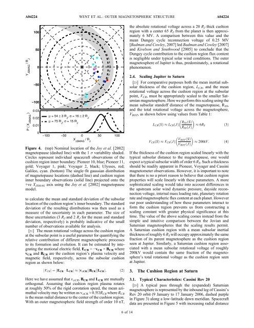
Figure 4. (top) Nominal location of the Joy et al. [2002]
magnetopause (dashed line) with the 1 s variability shaded.
Circles represent individual spacecraft observations of the
cushion region inner boundary: Pioneer 10, blue; Pioneer 11,
gold; Voyager 1, pink; Voyager 2, black; Ulysses, red;
Galileo, cyan. (bottom) The single‐fit gaussian distribution
of magnetopause locations (dashed line) and cushion region
inner boundary observations (solid line) projected onto the
+ve X JSMAG axis using the Joy et al. [2002] magnetopause
model.
to calculate the mean and standard deviation of the subsolar
location of the cushion region’s inner boundary. The standard
deviation of the resulting distributions was then used as a
measure of the uncertainty in each parameter. The size of
these uncertainties (3 R J and 2 R J for the mean and standard
deviation, respectively) is probably indicative of the small
number of observations available for analysis.
[21] The mean rotational voltage across the cushion region
at the subsolar point is a useful parameter for quantifying the
relative contribution of different magnetospheric processes
to its formation and evolution. It can be estimated by integrating
the motional electric field, E CR = −v CR × B CR where
v CR and B CR are the cushion region’s plasma velocity and
magnetic field, respectively, across the subsolar cushion
region as shown below:
jV CR j¼jE CR L CR jjv CR jjB CR jjL CR j:
Here we have assumed that v CR , B CR and L CR are mutually
orthogonal. Assuming that cushion region plasma rotates
at roughly 50% of the rigid corotation speed, the mean azimuthal
velocity may be written as v CR ≈ 0.5WR CR where R CR
is the mean radial distance to the center of the cushion region.
With an outer magnetospheric field strength of order 10 nT,
ð2Þ
V CR ðSÞ V CR ðJÞ
V
ROT ðSÞ
200kV:
ðJÞ
V ROT
If the thickness of the cushion region scaled linearly with the
typical subsolar distance to the magnetopause, one would
expect a typical subsolar width of order 6 R S . Such a thickness
should be readily apparent in Pioneer, Voyager and Cassini
magnetometer observations. However, it is important to note
that there is no a priori reason to believe that cushion region
properties will scale linearly with these parameters. A more
sophisticated scaling would take into account differences in
the upstream solar wind dynamic pressure, dayside reconnection
voltage, internal mass loading rate, planetary rotation
rate and magnetospheric flux content at each planet. However
our poor understanding of how these parameters interact to
form the cushion region prevents us from constructing a
scaling constant with greater physical significance at this
time. The value of the above scaling comes instead from the
simple and intuitive comparison between the Jovian and
Saturnian magnetospheres that the scaling results permit.
A Saturnian cushion region with a mean subsolar inertial
thickness of roughly 6 R S will occupy approximately the same
fraction of its parent magnetosphere as the cushion region
seen at Jupiter. Similarly, a Saturnian cushion region associated
with a mean subsolar rotational voltage of roughly
200kV would contain the same fraction of the magnetosphere’s
total rotational voltage as the cushion region seen
at Jupiter.
3. The Cushion Region at Saturn
3.1. Typical Characteristics: Cassini Rev 20
[25] A typical pass through the (expanded) Saturnian
magnetosphere is represented by the inbound leg of Cassini’s
Rev 20 orbit (9 January to 17 January 2006, dashed purple
in Figure 3) along a low‐latitude dawn meridian. Spacecraft
data are presented in Figure 5 with increasing radial distance
ð4Þ
6of14