The Quantum Mechanics of Global Warming - University of Virginia

The Quantum Mechanics 

of 

Global Warming 

Brad Marston 

Brown University 

University of Virginia 

April 17, 2009

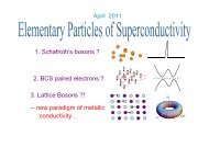
Richardson’s Human Weather Computer (1917 --1922) 

“Lewis Fry Richardson’s imaginary `forecast factor’ would have employed some 64,000 human 

computers to keep up with the pace of the weather, The workers sit in tiers inside a great 

spherical theater; the director, atop a pedestal in the middle, shines a beam of light on those 

places where the calculation is getting ahead or falling behind.” [Brian Hayes, American Scientist 

80, 10 -- 14 (2001).]

cooler sun 

continental drift 

orogeny 

climate 

optimum 

LIA 

synoptic 

disturbances

Outline

Outline 

• Quantum Mechanics #1: blackbody radiation

Outline 

• Quantum Mechanics #1: blackbody radiation 

• QM #2: Why we aren’t freezing

Outline 


• QM #2: Why we aren’t freezing 

• QM #3: Deciphering ice and sediment records

Outline 



• QM #3: Deciphering ice and sediment records 

• Fluid Dynamics: Single layer models 

• Coriolis Force 

• Stratification & Differential Heating 

• Topography

Outline 







• Topography 

• Quantum field theory of global warming?

Outline 







• Topography 

• Quantum field theory of global warming? 

• Ecosystems and feedbacks

Crisis in 19th Century Classical Physics

Crisis in 19th Century Classical Physics 

Intensity = function(T emperature, frequency)


Intensity = function(T emperature, frequency) 

[I] = W atts 

meter 2 = Joules 

m 2 s



[I] = W atts 


m 2 s 

[k B T ] = J



[I] = W atts 


m 2 s 

[k B T ] = J [ν] = 1 s



[I] = W atts 


m 2 s 

[k B T ] = J [ν] = 1 s 

c = 3 × 10 8 m/s speed of light 

k B = 1.38 × 10 −23 J/K Boltzmann ′ s constant



[I] = W atts 


m 2 s 

[k B T ] = J [ν] = 1 s 


k B = 1.38 × 10 −23 J/K Boltzmann ′ s constant 

∆I(T, ν) ∝ k BT ν 2 

∆ν 

c 2



[I] = W atts 


m 2 s 

[k B T ] = J [ν] = 1 s 



∆I(T, ν) ∝ k BT ν 2 

c 2 ∆ν I = 

∞∑ 

∆I(T, ν) → ∞ 

ν=0



[I] = W atts 


m 2 s 

[k B T ] = J [ν] = 1 s 



∆I(T, ν) ∝ k BT ν 2 

c 2 ∆ν I = 

∞∑ 

∆I(T, ν) → ∞ 

ν=0 

UV Catastrophe!

The Solution: Quanta

The Solution: Quanta 

Light is composed of 

particles -- quanta -- 

called photons. 

ɛ = hν Photons carry energy. 

h = 6.63 × 10 −34 Js Planck ′ s constant






h = 6.63 × 10 −34 Js Planck ′ s constant 

New constant of 

nature makes it 

possible to write 

the correct intensity. 

∆I(T, ν) = 2πhν3 

c 2 1 

e hν/k BT 

− 1 ∆ν 

→ 2πk BTν 2 

→ 

c 2 

0 for ν →∞ 

∆ν for k B T ≫ hν






h = 6.63 × 10 −34 Js Planck ′ s constant 

New constant of 

nature makes it 

possible to write 

the correct intensity. 

∆I(T, ν) = 2πhν3 

c 2 1 

e hν/k BT 

− 1 ∆ν 


→ 

c 2 

0 for ν →∞ 

∆ν for k B T ≫ hν 

Now we can 

do that sum 

over frequency! 

I = σT 4 

σ ≡ 2π5 kB 

4 W 

15h 3 =5.67 × 10−8 

c2 m 2 K 4

∆I(T, ν) = 2πhν3 

c 2 1 

e hν/k BT 

− 1 ∆ν 


→ 

c 2 

0 for ν →∞ 

∆ν for k B T ≫ hν 

Agree to better than 

1 part in 100,000

Temperature of the Earth 

Rsun 

The earth is (almost) in a thermal 

steady state: it emits as much radiation 

as it receives from the sun. 

r E 

RE


Rsun 




r E 

Albedo = a = 30%visible light 

reflected directly back to space 

(“earthshine” on the new moon). 

RE


Rsun 




r E 

Albedo = a = 30%visible light 

reflected directly back to space 

(“earthshine” on the new moon). 

fraction = πR2 E 

4πr 2 E 

× (1 − a) 

RE

Energy Balance 

Luminosity = Area × Intensity 

= 4πR 2 sun × σT 4 sun



= 4πR 2 sun × σT 4 sun 

incoming 

energy flux




incoming 

energy flux 

πR 2 E 

4πr 2 E 

(1 − a) 4πR 2 sun σT 4 sun = 4πR 2 E σT 4 E




Space 

incoming 

energy flux 

outgoing 

energy flux (IR) 

πR 2 E 

4πr 2 E 





Space 

incoming 

energy flux 

outgoing 


πR 2 E 

4πr 2 E 





Space 

incoming 

energy flux 

outgoing 


πR 2 E 

4πr 2 E 

(1 − a) 4πR 2 sun σT 4 sun = 4πR 2 E σT 4 E 

r E = 150 × 10 9 m 

R sun = 6.96 × 10 8 m 

T sun = 5, 800K



incoming 

energy flux 


Space 

outgoing 


πR 2 E 

4πr 2 E 


r E = 150 × 10 9 m 

R sun = 6.96 × 10 8 m 

T sun = 5, 800K 

√ 

T E = (1 − a) 1/4 Rsun 

2r E 

≈ 251K = −22C 

T sun



incoming 

energy flux 


Space 

outgoing 


πR 2 E 

4πr 2 E 


r E = 150 × 10 9 m 

R sun = 6.96 × 10 8 m 

T sun = 5, 800K 

√ 

T E = (1 − a) 1/4 Rsun 

2r E 

≈ 251K = −22C 

T sun 

FREEZING

Terrestrial Planets

Planet Earth Mars Venus 

calculated 

temperature 

actual 

temperature 

-18 0 C -56 0 C -39 0 C 

15 0 C -53 0 C 427 0 C 

greenhouse 

warming 33 0 C 3 0 C 466 0 C


calculated 

temperature 

actual 

temperature 

-18 0 C -56 0 C -39 0 C 

15 0 C -53 0 C 427 0 C 

greenhouse 

warming 33 0 C 3 0 C 466 0 C


calculated 

temperature 

actual 

temperature 

-18 0 C -56 0 C -39 0 C 

15 0 C -53 0 C 427 0 C 

greenhouse 

warming 33 0 C 3 0 C 466 0 C


calculated 

temperature 

actual 

temperature 

-18 0 C -56 0 C -39 0 C 

15 0 C -53 0 C 427 0 C 

greenhouse 

warming 33 0 C 3 0 C 466 0 C 

Water Vapour: 65% Carbon Dioxide: 21%

Why We Aren’t Freezing 

from Climate Change 1995: The Science of Climate Change

H2O 

hν 

- 

+ + 

hν 

hν = Ef - Ei

H2O 

hν 

- 

+ + 

hν 

hν = Ef - Ei 

CO2 

- + 

-

H2O 

hν 

- 

+ + 

hν 

hν = Ef - Ei 

CO2 

N2 

O2 

Ar 

- + 

- 

Transparent

Principal greenhouse 

gas: water vapor 

Secondary: carbon 

dioxide, methane, 

CFC’s, … 

Robert A. Rohde for the Global Warming Art project





CFC’s, … 

Absorption lines are 

pressure-broadened 






CFC’s, … 

Absorption lines are 

pressure-broadened 

IR photons are on 

average absorbed and 

emitted about 2x on 

way out to space 


John Harte, Consider a Spherical Cow

Ω = 1372 W/m 2 

John Harte, Consider a Spherical Cow

John Harte, Consider a Spherical Cow 

Ω = 1372 W/m 2 Ω 

4 

= a Ω 4 + σT 4 0 + F w 

2σT 4 0 = σT 4 1 + 0.5F e + 0.7F s 

2σT 4 1 = σT 4 0 + σT 4 s − F w + F c + 0.5F e + 0.3F s


Ω = 1372 W/m 2 Ω 

4 

= a Ω 4 + σT 4 0 + F w 

2σT0 4 = σT1 4 + 0.5F e + 0.7F s 

2σT1 4 = σT0 4 + σTs 4 − F w + F c + 0.5F e + 0.3F s 

F s ≈ 86 W/m 2 Solar flux absorbed by atmosphere 

F e ≈ 80 W/m 2 Latent heat from evaporating water 

F w ≈ 20 W/m 2 IR flux directly to space 

F c ≈ 17 W/m 2 Convective heat transfer


Ω = 1372 W/m 2 Ω 

4 

= a Ω 4 + σT 4 0 + F w 

2σT 4 0 = σT 4 1 + 0.5F e + 0.7F s 

2σT1 4 = σT0 4 + σTs 4 − F w + F c + 0.5F e + 0.3F s 

T 

F s ≈ 86 W/m 2 0 = 250K 

Solar flux absorbed by atmosphere 

T 

F e ≈ 80 W/m 2 1 = 278K 

Latent heat from evaporating water 

T 

F w ≈ 20 W/m 2 s = 289K = 16C 

IR flux directly to space 

F c ≈ 17 W/m 2 Convective heat transfer 

Excellent agreement 

for such a simple model

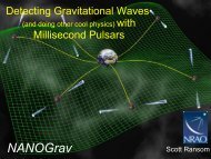
Tropopause 

Z e Z e + !Z e 

Held & Soden (2000) 

Altitude 

1xCO 2 

2xCO 2 

Temperature 

T e 

T s 

T s + !T s 

Figure 1 Schematic illustration of the change in emission level (Z e ) associated with an 

increase in surface temperature (T s ) due to a doubling of CO 2 assuming a fixed atmospheric 

lapse rate. Note that the effective emission temperature (T e ) remains unchanged.

The Past 160,000 Years 

J. M. Barnola et al., Nature 329, 408 (1987) 

Carbon Dioxide 

Temperature 

Present

Quantum Zero-Point Motion 

(Harold Urey, “The thermodynamic properties of isotopic substances,” 1946)


Classically: All motion ceases at absolute zero temperature. 

Everything freezes into a solid. 





Quantum physics: There is still some motion even at T = 0. 

This is why liquid helium never freezes! 







Small mass --> large 

quantum zero-point 

motion and energy. 

ν = 1 

2π 

√ 

2k 

m 

E 0 = 1 2 hν 

m 

k 

m 

He 







Small mass --> large 

quantum zero-point 

motion and energy. 

ν = 1 

2π 

√ 

2k 

m 

E 0 = 1 2 hν 

m 

k 

m 

He 

18O versus 16O in H2O: Classically both molecules have same energy. 

Quantum zero-point energy means that 18O water is slightly less likely 

to evaporate during cold spells. 


S. J. Johnsen et al. Tellus 41B, 452 (1989)

Eccentricity: 100 and 413 kyr 

N 

S

α Draconis 

(2000 BC) 

Polaris 

(now) 

Precession: 19 to 23 kyr 


N 

S

α Draconis 

(2000 BC) 

Polaris 

(now) 

Precession: 19 to 23 kyr 


N 

23.5o (now) 

ecliptic 

S 

Change in tilt of axis 

“obliquity”: 41 kyr

Spectral Analysis of Isotope Records 

Figures from Ice Ages and 

Astronomical Causes: Data, 

Spectral Analysis, and Mechanisms 

by R. Muller and G. MacDonald

Spectral Analysis of Isotope Records 

Figures from Ice Ages and 

Astronomical Causes: Data, 

Spectral Analysis, and Mechanisms 

by R. Muller and G. MacDonald

What amplifies orbital 

forcing to produce 

ice ages?



ice ages? 

Why does 100 kyr 

eccentricity period 

dominate climate signal?



ice ages? 

Why does 100 kyr 

eccentricity period 

dominate climate signal? 

Why did the 41 kyr 

period dominate 1.5 

million years ago?

Martian Climate May Also 

Show Orbital Forcing 

North Polar Cap of Mars 

Laskar, Levrard, and Mustard, 

Nature 419, 375 (2002); Head 

et al. Nature 426, 797 (2003).

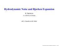
D. Lüthi et al. Nature 453, 379 (2008) 

26

LIDE 7 

Ice Age Climate Forcings (W/m 2 ) 

aerosols 

greenhouse 

ice sheets gases 

& 

vegetation CO 2 

-0.5 ± 1 

CH 4 

N 2 O 

-2.6 ± 0.5 

-3.5 ± 1 

Fig 2. Global radiative forcings during the last ice age relative to the current 

interglacial period. The total forcing is -6.6 ± 1.5 W/m 2 . Thus, the 5°C cooling 

of the ice age implies a climate sensitivity of 0.75°C per 1 W/m 2 forcing. 

Hansen, J. et al., The missing climate forcing, Phil. Trans. R. Soc. London. B, 352, 231-240, 1997.

Atmospheric Dynamics 

from Climate Change 1995: 

The Science of Climate Change

Single Layer Models

Single Layer Models 

Dω 

Dt =0


Vorticity 

Dω 

Dt =0 

ω = ˆr · ( ⃗ ∇×⃗v)


Vorticity 

Dω 

Dt =0 

ω = ˆr · ( ⃗ ∇×⃗v) 

∂ω 

∂t + ⃗v · ⃗∇ω =0 

⃗v = ˆr × ⃗ ∇ψ 

⃗∇· ⃗v = 0 

ω = ∇ 2 ψ


Vorticity 

Dω 

Dt =0 

ω = ˆr · ( ⃗ ∇×⃗v) 

∂ω 

∂t + ⃗v · ⃗∇ω =0 

∂ω 

∂t 

+ J(ψ, ω) = 0 

⃗v = ˆr × ⃗ ∇ψ 

⃗∇· ⃗v = 0 

J(ψ, ω) ≡ ∂ψ 

∂x 

∂ω 

∂y − ∂ψ 

∂y 

∂ω 

∂x 

ω = ∇ 2 ψ

Freely Decaying Turbulence 

on Sphere

Coriolis Force

Coriolis Force 

∂q 

∂t 

+ J(ψ, q) = 0


∂q 

∂t 

+ J(ψ, q) = 0 

Relative vorticity 

q = ω + f 

Coriolis term 

Absolute 

vorticity 

= ∇ 2 ψ + f


∂q 

∂t 

+ J(ψ, q) = 0 

Relative vorticity 

q = ω + f 

Coriolis term 

Absolute 

vorticity 

= ∇ 2 ψ + f 

f = 2Ω sin(φ)

Coriolis Force

Chelton et al., Science 303, 978 (2004)

Stratification

Stratification 

q = ∇ 2 ψ + f − ψ l 2 R


q = ∇ 2 ψ + f − ψ l 2 R 

l 2 R = gh 

f 2


q = ∇ 2 ψ + f − ψ l 2 R 

l 2 R = gh 

f 2 

h 

l R = O(1, 000 km)

Stratification Sets Synoptic Length 

Scale

Stratification Sets Synoptic Length 

Scale

7. The NADW Meridional Cell and Deep Western Boundary Current 

b -,c. 

Q. '" 

=~ ,,-a 

Figure 1-91 : A new version of 

Figure 1-90 with schematic 

meridional sections of 

interbasin flow for each ocean 

with their global linkages. 

SAMW 

AAIW 

RSOW 

AABW 

NPDW 

AAC 

CDW 

NADW 

UPPER IW 

IODW 

Subantarctic Mode Water 

Antarctic Intermediate Water 

Red Sea Overflow Water 

Antarctic Bottom Water 

North Pacific Deep Water 

Antarctic Circumpolar Current 

Circumpolar Deep Water 

North Atlantic Deep Water 

26.8:: (Je:: 27.25 

Indian Ocean Deep Water 

W. J. Schmitz, WHOI technical report 96-03 

There is a recent review article on NADW (Fine, 1995) containing a schematic

City Latitude January ( o F) August ( o F) 

Glasgow 56 o 34 to 45 52 to 64 

Sitka 57 o 30 to 38 52 to 62


Glasgow 56 o 34 to 45 52 to 64 

Sitka 57 o 30 to 38 52 to 62


Glasgow 56 o 34 to 45 52 to 64 

Sitka 57 o 30 to 38 52 to 62

Topography & Angular Momentum 

Richard Seager, “The Source of Europe’s Mild 

Climate,” American Scientist (July-August 2006)

Quantum Field Theory 

of Global Warming? 

"More than any other theoretical procedure, 

numerical integration is also subject to the criticism 

that it yields little insight into the problem. The 

computed numbers are not only processed like data 

but they look like data, and a study of them may be 

no more enlightening than a study of real 

meteorological observations. An alternative 

procedure which does not suffer this disadvantage 

consists of deriving a new system of equations 

whose unknowns are the statistics themselves." 

Edward Lorenz, The Nature and Theory of the General Circulation (1967)

PV = nRT

PV = nRT 

Thermodynamics vs. Statistical Mechanics

PV = nRT 

Thermodynamics vs. Statistical Mechanics 

Equilibrium vs. Out-of-Equilibrium

PV = nRT 

Thermodynamics vs. Statistical Mechanics 

Equilibrium vs. Out-of-Equilibrium

Hopf Functional Approach

Hopf Functional Approach 

dx 

dt = x2


dx 

dt = x2 

Ψ(t, u) ≡ e iux(t)


dx 

dt = x2 

Ψ(t, u) ≡ e iux(t) 

i ∂ ∂t 

Ψ= u 

∂2 

∂u 2 Ψ


dx 

dt = x2 


i ∂ ∂t 

Ψ= u 

∂2 

∂u 2 Ψ 

i ∂ ∂t 

Ψ= u 

∂2 

∂u 2 Ψ


dx 

dt = x2 


i ∂ ∂t 

Ψ= u 

∂2 

∂u 2 Ψ 

i ∂ ∂t 

Ψ= u 

∂2 

∂u 2 Ψ 

ĤΨ 0 = 0 

Ψ 0 (u) = exp{iu〈x〉− 1 2! u2 (〈x 2 〉−〈x〉 2 )+...} 

〈x〉 = −i ∂Ψ 0(u) 

∂u 

∣ 

u=0

A. Sanchez-Lavega et al. Nature 451, 437 (2008)

0 

A. Sanchez-Lavega et al. Nature 451, 437 (2008) 

10 -6 -40 

Mean Zonal Velocity

0 

A. Sanchez-Lavega et al. Nature 451, 437 (2008) 

Mean Zonal Velocity

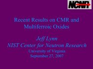
Direct Numerical Simulation of Jet 

jet relaxation time = 25 days 

J. B. M, E. Conover, and T. Schneider, J. Atmos. Sci. 65, 1955 (2008)

Direct Numerical Simulation of Jet 

jet relaxation time = 25 days 

FIG. J. 1. B. Absolute M, E. Conover, vorticity qand as calculated T. Schneider, by DNS J. Atmos. for a jetSci. relaxation 65, 1955 time(2008) 

of τ = 25 days

1.5625 days 

12.5 days 

3.125 days 

25 days 

6.25 days 

50 days

10 -5 -10 

10 

8 

(a) 

Mean Absolute Vorticity (1/s) 

6 

4 

2 

0 

-2 

-4 

-6 

-8 

! = 0 days 

DNS: ! = 1.5625 days 

CE: ! = 1.5625 days 

DNS: ! = 3.125 days 

CE: ! = 3.125 days 

DNS: ! = 6.25 days 

CE: ! = 6.25 days 

DNS: ! = 25 days 

CE: ! = 25 days 

-70 -60 -50 -40 -30 -20 -10 0 10 20 30 40 50 60 70 

Latitude (degrees) 

10 -6 -20 

20 

15 

(b) 

Mean Absolute Vorticity (1/s) 

10 

5 

0 

-5 

-10 

-15 

-20 -15 -10 -5 0 5 10 15 20 

Latitude (degrees)

2nd Cumulant = 2-point Correlation Function

25 days

Ecosystems & Feedbacks 

C. D. Keeling and T. P. Whorf 

Hawaii 

Antarctica

Ecosystems & Feedbacks 

C. D. Keeling and T. P. Whorf 

Amplitude of 

seasonal cycle 

is growing. 

Hawaii 

Antarctica

Vast Reservoirs of Carbon & Enormous Fluxes 

Source: Climate Change 1995

J. B. Marston, M. Oppenheimer, R. M. Fujita, and S. R. Gaffin, “CO2 and temperature” 

Nature 349, 573 (1991).

Physics of Feedbacks 

Input (I) 

System 

Output (O) 

gain (g)


Input (I) 

System 

Output (O) 

gain (g) 

O = I + gI + ggI + ··· 

= 

I 

1 − g 

if g


Input (I) 

System 

Output (O) 

gain (g) 

O = I + gI + ggI + ··· 

= 

I 

1 − g 

if g

Some Feedbacks Already Included in Models

Some Feedbacks Already Included in Models 

Feedback Process 

Gain g 

water vapor 0.40 (0.28 to 0.52) 

ice & snow 0.09 (0.03 to 0.21) 

clouds 0.22 (-0.12 to 0.29) 

Total 0.71 (0.17 to 0.77)



Gain g 

water vapor 0.40 (0.28 to 0.52) 

ice & snow 0.09 (0.03 to 0.21) 

clouds 0.22 (-0.12 to 0.29) 

Total 0.71 (0.17 to 0.77)



Gain g 

water vapor 0.40 (0.28 to 0.52) 

ice & snow 0.09 (0.03 to 0.21) 

clouds 0.22 (-0.12 to 0.29) 

Total 0.71 (0.17 to 0.77)



Gain g 

water vapor 0.40 (0.28 to 0.52) 

ice & snow 0.09 (0.03 to 0.21) 

clouds 0.22 (-0.12 to 0.29) 

Total 0.71 (0.17 to 0.77)



Gain g 

water vapor 0.40 (0.28 to 0.52) 

ice & snow 0.09 (0.03 to 0.21) 

clouds 0.22 (-0.12 to 0.29) 

Total 0.71 (0.17 to 0.77)



Gain g 

water vapor 0.40 (0.28 to 0.52) 

ice & snow 0.09 (0.03 to 0.21) 

clouds 0.22 (-0.12 to 0.29) 

Total 0.71 (0.17 to 0.77) 

∆T ≈ 1 ◦ C/(1 − 0.71) ≈ 3.4 ◦ C

IPCC 2001

IPCC 2001

Global Carbon Cycle 

Small change in g causes large ΔT 

Asymmetries 

Decrease in warming due 

to ecosystem feedbacks 

Extra warming due to 

ecosystem feedbacks 

ΔT (ºC) 

due to 

feedback 

2×CO 2 g = 0.7 

(no eco feedbacks) 

Change in g 

due to ecosystem feedbacks 

M.S. Torn, LBNL

An estimate of the contribution to g from Vostok core data: 

Torn and Harte, GRL33, 

L10703 (2006) 

CO 2 (ppm) 

Holocene CO 2 -Temp coupling 

General 

Circulation 

Models 

M.S. Torn, LBNL 

Data Cuffey & Vimeux 2002 

ΔT (K) 

g CO2 = ∂T 

∂[CO 2 ] · ∂[CO 2] 

∂T 

= 1◦ C 

275ppmv · 14.6ppmv 

1 ◦ C 

=0.053 

1 o C/(1 - .71) = 3.4 o C 

1 o C/(1 - .71 – .05) = 4.2 o C 

But where is the carbon 

coming from?

(a) 

.6 

.4 

Global Temperature Change (C) 

Annual Mean 

5-year Mean 

.2 

.0 

-.2 

-.4 

1880 1900 1920 1940 1960 1980 2000

Source: Global Warming Art

What Can Modern Physics Contribute?

What Can Modern Physics Contribute? 

Aspen Center for Physics 

Summer 2005 Workshop 

Novel Approaches To Climate 

Funding: NSF, BP Research, & ICAM 

John Harte’s long-term ecosystem heating 

experiment at the Rocky Mountain 

Biological Laboratory near Aspen.

What Can Modern Physics Contribute? 

Aspen Center for Physics 

Summer 2005 Workshop 

Novel Approaches To Climate 

Funding: NSF, BP Research, & ICAM 

Kavli Institute for Theoretical Physics 

Physics of Climate Change 

April 28 -- July 11, 2008 

Frontiers of Climate Science 

& Engineering the Earth 

May 6 -- 10, 2008 

John Harte’s long-term ecosystem heating 

experiment at the Rocky Mountain 

Biological Laboratory near Aspen. 

Co-organizers: 

J. Carlson, G. Falkovich, J. Harte, 

J. B. Marston, and R. Pierrehumbert

“Human beings are now 

carrying out a large scale 

geophysical experiment of a 

kind that could not have 

happened in the past nor be 

reproduced in the future. 

Within a few centuries we are 

returning to the atmosphere 

and oceans the concentrated 

organic carbon stored in 

sedimentary rocks over 

hundreds of millions of years. 

(Revelle and Suess, 1957)

scent of the n 5/3 

tional data near the 

but here it is more 

eractions prevent a 

all length scales. 

nergy spectrum is 

tions over a wide 

paradox that the 

wer-law decay that 

in an inertial range 

in the atmospheric 

elated to eddy-eddy 

other terms would 

spectrum. We also 

eter settings in the 

d and Suarez, 1994] 

layer schemes and 

, our results for the 

artifacts of specific 

. The approximate 

ut eddy-eddy interventional 

enstrophy 

nent plays a central 

t this is difficult to 

erms in the spectral 

nly considered the 

s may apply to the 

Figure 3. Mean eastward wind (m s 1 ) in the meridional 

plane in (a) the full simulation and (b) the simulation 

without eddy-eddy interactions. The mean is a zonal, time, 

and interhemispheric average with mass weighting. The 

thick solid lines are the zero-wind lines.

Antarctic Dome C 

Siegenthaler et al. Science 310, 1313 (2005)

Antarctic Dome C 

Siegenthaler et al. Science 310, 1313 (2005)

Lake Mead

The Quantum Mechanics of Global Warming - University of Virginia

Create successful ePaper yourself

Delete template?

Save as template?